Research on Injection Profile Interpretation Method Based on DTS Logging

Abstract

Distributed temperature sensing (DTS) has been widely used in downhole dynamic monitoring. How to analyze its data and accurately interpret the flow profile using DTS data are still great challenges. Quantitative interpretation of downhole temperature measurements requires the development of an integrated flow and thermal model capable of handling multi-phase flow. The model must strike a balance between computational efficiency and achieving the highest possible accuracy. The finite difference method can solve the relevant problems well. The flow model and thermal model of reservoirs and wellbores are established. Combined with the single-phase flow theory, the coupling prediction model of wellbore and reservoir temperature is established through appropriate boundary and constraint conditions. The problem was solved iteratively using the finite difference method, and the coupled temperature prediction model’s reliability was confirmed through comparison with numerical simulation results. Based on the forward model, the sensitivity analysis of the influencing factors is carried out in this study which provides a theoretical basis for the inversion model. Taking the flow rate as the inversion parameter, the injection profile interpretation model based on DTS logging data is constructed. Four optimization methods are used in the inversion model which can balance the computational efficiency and model accuracy. The DTS data are preprocessed by the Kalman filter, and the inversion and interpretation evaluation of X injection well is carried out by the LSO-MCMC combined optimization algorithm. The results show that the method has high reliability in the interpretation accuracy of injection profile, and the inverted flow profile meets practical application requirements, confirming the method’s accuracy and effectiveness.

1. Introduction

Downhole temperature monitoring, as one of the diagnosis tools, has been widely used. DTS technology obtains temperature data by measuring changes in Raman scattered signals. As an important geological exploration tool, well temperature logging can be traced back to the middle of the 20th century [1]. In the past few decades, the heat transfer mechanism between a wellbore and formation has been studied (Hasan, 1994) and the wellbore temperature field theoretical model (Kabir, 2002) has been used to carry out a large number of studies [2,3]. Additionally, Yoshioka et al. (2007) proposed a steady-state temperature model for horizontal well profiling [4]. Sui et al. (2012) developed a transient wellbore and reservoir thermal model for vertical wells, and the model has been applied to characterize near-wellbore damage [5].

Hasan et al. (2010) calculated the pressure and temperature of the casing annulus according to the heat transfer theory and estimated the flow rate in the calculation process [6]. Li et al. (2010) established a horizontal well temperature model in water drive reservoir which was used as a forward modeling model, and they established an inversion model based on the MCMC algorithm [7]. Through inversion of temperature data, the output profile was obtained. Among production well models, the semi-analytical model offers high computational speed but is limited to single-phase flow in homogeneous reservoirs. In contrast, the fully numerical compositional model (Yoshida and Hill, 2016) accommodates multi-phase flow and heterogeneous formations but is constrained by low computational efficiency [8]. To achieve effective temperature interpretation with thermal models, it is crucial to balance computational efficiency and model robustness. Zhu Shiyan (2016) established horizontal well DTS data inversion models based on the L-M and MCMC algorithms, respectively, but they were only applicable to homogeneous reservoirs [9]. Chen Lin et al. (2017) proposed a new method for calculating the wellbore temperature and pressure profile and they established a coupling model of wellbore temperature and pressure in the case of gas production, but this model is only applicable to the unsteady flow model of gas wells [10]. Li Haitao et al. (2021) developed a temperature prediction model for fractured horizontal wells and established a DTS data inversion model using the MCMC algorithm, providing significant support for evaluating the fracturing reconstruction effects in shale gas reservoirs. However, the application of this model has been limited to only a few measured wells [7]. Luo et al. (2021) established DTS data inversion models based on the MCMC algorithm and SA algorithm, respectively, proposed the method for selecting initial values of inversion target parameters, and optimized the inversion process, but there were few interpretation applications [11]. Huang Liang et al. (2024) established a multi-phase flow wellbore temperature distribution model and optimized the inversion model by using the PSO algorithm. However, the applicability is low and the accuracy needs to be further improved [12].

To enhance the accuracy and applicability of DTS log inversion interpretation, this study leverages the flexibility and robustness of the finite difference method (FDM) to iteratively solve a coupled temperature prediction model [13]. Under identical formation, fluid, and wellbore conditions, the FDM results were compared with numerical simulation outcomes to validate its feasibility. Building on the forward model, an inversion interpretation model for injection profiles was established and the performance of the MCMC and L-M algorithms was evaluated. The stochastic-based MCMC algorithm was selected for its superior inversion effect, and four strategies to improve inversion efficiency were proposed. By refining grid discretization, optimizing the inversion algorithm, and adjusting convergence criteria, the global search LSO algorithm was introduced to optimize the inversion model, thereby balancing computational efficiency and accuracy. To improve DTS data quality, the impact of data noise on reading speed and interpretation results was investigated, and data preprocessing techniques were applied to enhance data quality, ultimately improving the accuracy of DTS log inversion interpretation. This research culminates in a comprehensive quantitative method for interpreting injection profiles based on DTS log data.

2. Description of Models

The forward model describes fluid temperature and pressure variations during water injection flow, assuming a vertical well fully penetrates a uniform rectangular reservoir. The well’s flow process is characterized by mass and momentum balance equations, while temperature changes are represented by the energy balance equation [14].

2.1. Wellbore Model

2.1.1. Mass Balance

The wellbore flow model is a crucial tool for characterizing fluid flow and heat transfer behavior within the wellbore [15]. Analyzing the pressure distribution enables the inference of fluid flow direction and flow rate distribution. The mass balance equation is a core component of establishing wellbore flow models and is suitable for describing the mass distribution and variation characteristics of single-phase or multi-phase fluid flow. The aforementioned equation may be articulated as [10]:

$$\pi r^2\Delta \mathrm{z}{\displaystyle \frac{\partial \rho }{\partial t}}=-2\pi r\gamma ({\rho }_I{v}_I)+\pi r^2{(\rho v)}_z-\pi r^2{(\rho v)}_{z+\Delta \mathrm{z}}$$

(1)

where under steady-state conditions, the velocity at node i within the wellbore can be determined utilizing the subsequent formula:

$${\nu }_{i+1/2}={\displaystyle \frac{{\rho }_{i-1/2}{\nu }_{i-1/2}}{{\rho }_{i+1/2}}}-{\displaystyle \frac{\Delta z_i}{{\rho }_{i+1/2}}}{\displaystyle \frac{2\gamma }{r}}{({\rho }_I{\nu }_I)}_i$$

(2)

where $v$—axial velocity (m/s);

• $v_I$—radial velocity (m/s);
• $r$—wellbore radius (m);
• $\gamma$—pipe open ratio;
• $\rho$—density (kg/m³).

2.1.2. Momentum Balance

The wellbore momentum balance is used to analyze the various forces and pressure distribution that a fluid experiences in the wellbore. The equation is expressed as:

$$\rho \pi r^{2}dz\left({\displaystyle \frac{\partial v}{\partial t}}+v{\displaystyle \frac{\partial v}{\partial z}}\right)=\rho g\cos \theta \pi r^{2}dz+p\pi r^2-\left(p+{\displaystyle \frac{\partial p}{\partial z}}dz\right)\pi r^2-{\displaystyle \frac{1}{2}}f\rho v^2\cdot 2\pi rdz$$

(3)

where the aforementioned equation can be formally expressed as: total pressure drop = gravity-induced pressure drop + acceleration-induced pressure drop + frictional pressure drop [16]. By solving the steady-state momentum balance equation by difference and sorting it out, the calculation formula of i + 1 node pressure in the wellbore is as follows:

$$p_{i+1}^{n+1}=p_i^{n+1}-\Delta z_{i+1/2}\left[-{\displaystyle \frac{{(\rho f{v}^2)}_{i+1/2}^{n+1}}{\mathrm{r}}}+{\displaystyle \frac{2\gamma }{R}}{\left({\rho }_I{v}_{I}v\right)}_{i+1/2}^{n+1}-{(\rho v)}_{i+1/2}^{n+1}{\displaystyle \frac{v_{i+1}^{n+1}-v_i^{n+1}}{\Delta z_{i+1/2}}}+{(\rho g\cos \theta )}_{i+1/2}\right]$$

(4)

where $f$—coefficient of friction;

• $m$—mixed fluid;
• $p$—pressure (MPa);
• $D$—the vertical depth calculated from a certain reference plane, with the downward direction being positive (m);
• $g$—gravitational acceleration (m/s²).

2.1.3. Energy Balance

The wellbore thermal model is established based on energy conservation, taking into account the kinetic energy, potential energy, internal energy of the fluid, and energy loss along the wellbore. The differential form of the energy balance equation of the wellbore model during injection is:

$${\displaystyle \frac{1}{\nu }}{\displaystyle \frac{\partial T}{\partial t}}={\displaystyle \frac{\beta T}{\rho \nu {\widehat{C}}_p}}{\displaystyle \frac{\partial p}{\partial t}}+{\displaystyle \frac{2\left(1-\gamma \right)}{r\rho \nu {\widehat{C}}_p}}\dot{q}-{\displaystyle \frac{\partial T}{\partial z}}+{\displaystyle \frac{\left(1-\beta T\right)}{\rho {\widehat{C}}_p}}{\displaystyle \frac{\partial p}{\partial z}}+{\displaystyle \frac{g\cos \theta }{{\widehat{C}}_p}}$$

(5)

where $\beta$—thermal expansion coefficient;

• $T$—temperature (°C);
• $C_p$—specific heat capacity (J/(kg·°C));
• $t$—time (s);
• $\dot{q}$—water injection volume per meter (m²/d).

The first term on the right side of the above equation is transient formation fluid gravitational expansion or compression (The first term on the right side of the above equation is the transient expansion or compression term of the formation fluid). The second term is heat convection. The third term is heat conduction. The fourth term is fluid expansion or compression and viscous dissipation [17]. The fifth item is gravitational energy. For water injection wells, considering that the reaction heat may have little effect on the results, the reaction heat term was not added in order to simplify the model. If the interpretation accuracy needs to be further improved, the reaction heat term should be added [18]. Assuming that the fluid in the wellbore and formation is stationary during the shut in period, with only thermal conduction present, the heat transfer model of the injection well during the shut in period is:

$$\rho {\widehat{C}}_p{\displaystyle \frac{\partial T}{\partial t}}=K_T{\displaystyle \frac{{\partial }^{2}T}{\partial z^2}}+{\displaystyle \frac{2}{R}}{U}_T\left({\left.T_r\right|}_{r=r_r}-T\right)$$

(6)

where $K_T$—thermal conductivity (J/(m·s·K));

• $U_T$—overall heat transfer coefficient (J/(m·s·K)).

2.2. Reservoir Model

2.2.1. Reservoir Seepage Model

A reservoir seepage model is developed based on the principle of mass balance to simulate fluid flow characteristics, pressure distribution, and flow rate variations within the reservoir [19]. The downhole fluid in the injection well is single-phase water, and the basic differential equations for two-phase seepage of water and oil are as follows:

$$\nabla \cdot \left[{\displaystyle \frac{{\rho }_{w}k{k}_{rw}}{{\mu }_w}}\left(\nabla p_w-{\rho }_{w}g\nabla D\right)\right]={\displaystyle \frac{\partial }{\partial t}}\left(\varphi {\rho }_w{S}_w\right)$$

(7)

$$\nabla \cdot \left[{\displaystyle \frac{{\rho }_{\mathrm{o}}k{k}_{\mathrm{ro}}}{{\mu }_{\mathrm{o}}}}\left(\nabla p_{\mathrm{o}}-{\rho }_{\mathrm{o}}g\nabla D\right)\right]={\displaystyle \frac{\partial }{\partial t}}\left(\varphi {\rho }_{\mathrm{o}}{S}_{\mathrm{o}}\right)$$

(8)

where $\varphi$—porosity;

• $S$—saturation;
• $k$—formation permeability (md);
• $k_{\mathrm{r}}$—relative permeability;
• $\mu$—viscosity (mPa·s);
• $g$—gravitational acceleration (m/s²).

If it is an oil–water two-phase production well, the finite difference method and implicit pressure explicit saturation method (IMPES) are used to solve Equations (7) and (8) in combination. During the closure of the injection well, there is no fluid flow in the wellbore and formation [20].

2.2.2. Reservoir Thermal Model

A reservoir thermal model is established based on energy balance considerations of heat conduction, convection, and the Joule–Thomson effect, which can describe the heat transfer laws between fluids, formations, and wellbore in the reservoir [21]. Assuming a flow rate injection, the reservoir heat transfer model during water injection can be expressed as:

$$\overline{\rho {\widehat{C}}_p}{\displaystyle \frac{\partial T}{\partial t}}=-{\displaystyle \frac{\rho {\widehat{C}}_p\dot{q}}{2\pi r}}{\displaystyle \frac{\partial T}{\partial r}}+K_T\left[{\displaystyle \frac{1}{r}}{\displaystyle \frac{\partial }{\partial r}}\left(r{\displaystyle \frac{\partial T}{\partial r}}\right)+{\displaystyle \frac{{\partial }^{2}T}{\partial z^2}}\right]$$

(9)

where the first term on the right side of the above equation is heat convection, and the second term is heat conduction, including radial heat conduction between the formation and the wellbore and axial heat conduction inside the wellbore. During the shutdown period, there is only heat conduction, which can be expressed as:

$$\overline{\rho {\widehat{C}}_p}{\displaystyle \frac{\partial T}{\partial t}}=K_T\left[{\displaystyle \frac{1}{r}}{\displaystyle \frac{\partial }{\partial r}}\left(r{\displaystyle \frac{\partial T}{\partial r}}\right)+{\displaystyle \frac{{\partial }^{2}T}{\partial z^2}}\right]$$

(10)

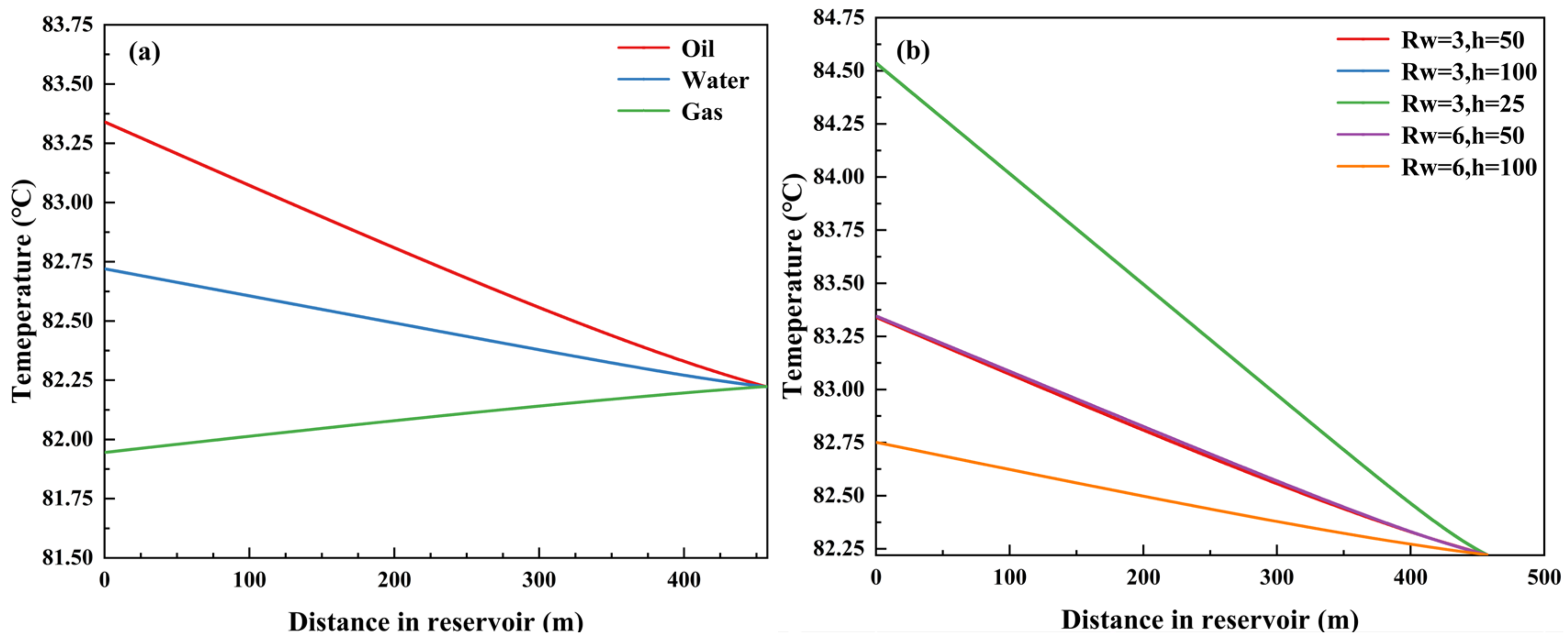
2.2.3. Inflow Temperature Model

An inflow temperature model can not only help to optimize water injection design, but also provide powerful theoretical support for flow monitoring, heat conduction analysis, and temperature distribution prediction of water injection wells.

The amount in the injection will affect the temperature change in the fluid as it passes through the porous medium. (The amount of injection will affect the temperature change as the fluid moves through the formation.) When the measured temperature of the water injection well deviates from the formation temperature, the injection volume can be determined according to the deviation degree of the measured temperature, which is helpful to monitor and evaluate the flow rate change in the water injection well. The formula for calculating fluid inflow temperature is as follows:

$$T_1={\displaystyle \frac{1}{\beta }}+(T_e-{\displaystyle \frac{1}{\beta }}){({\displaystyle \frac{r}{h/2}})}^{m_r}$$

(11)

where $T_I$—fluid inflow temperature (°C);

• $h$—reservoir thickness (m);
• $T_e$—intermediate parameters.

The reservoir parameters adopted in this paper include the following: permeability k is 50 md, formation length L is 304.8 m, formation width Y is 914.4 m, reservoir thickness is 15.24 m, outer boundary temperature is 82.2 °C, outer boundary pressure is 25.5 Mpa, and wellbore radius is 0.07 m.

Table 1. Physical parameters of downhole fluid properties.

Argument	Oil	Gas	Water
Viscosity (mPa·s)	22	0.0221	0.14
Specific heat capacity (J/(g·°C))	2000	2556	4234
Density (g/m)	950	0.9	1001
Coefficient of thermal expansion (1/°C)	0.000202	0.005	0.0004
Thermal conductivity (W/(m·°C))	0.14	2.63	0.609
Volume coefficient (m3/m3)	1.37	0.005	1.02

shows the physical parameters of downhole fluids, which are provided under standard temperature and atmospheric pressure (Yoshioka, 2007) [4]. When the temperature and pressure change, the fluid physical parameters need to be updated and iterated according to the calculation formula.

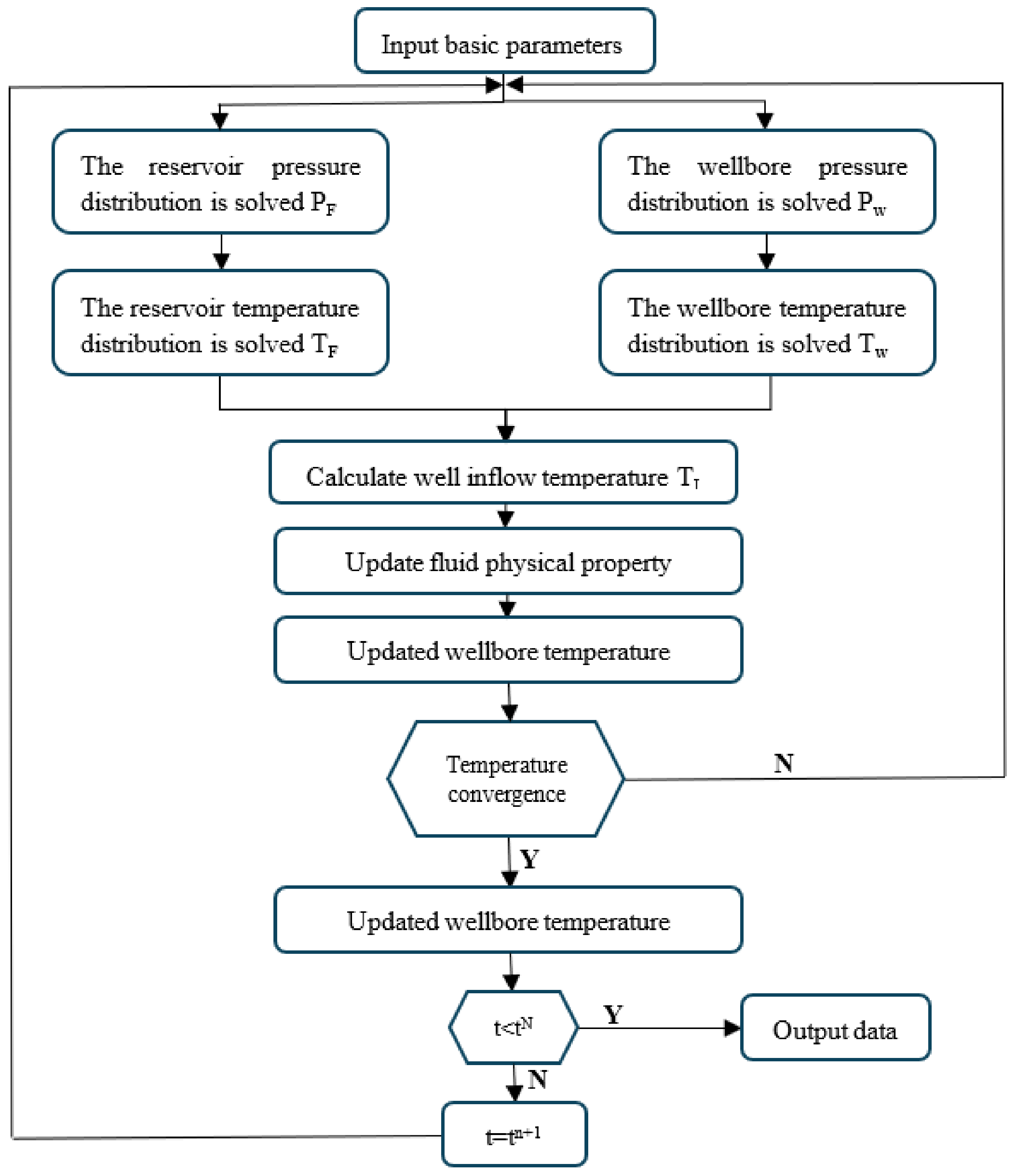
2.3. Solution Procedure for the Coupled Model

In actual production, the formation and wellbore constitute a complete system. After we have established the separate wellbore and reservoir models described above, we must couple the two together to calculate accurate transient temperatures. Solving the coupling model mainly includes the following three key steps: (1) using the initialization parameters to solve the results of time point n, (2) using the results to initialize the parameters of time point n + 1, and (3) solving the results of time point n + 1, as shown in the program flow chart below. In addition to establishing the coupling model, appropriate boundary and initial conditions are also essential for the precise constraints of the model, and optimizing the initial conditions can significantly improve the accuracy of interpretation results.

3. Models Validation

3.1. Inflow Temperature

Figure 1 shows the reservoir fluid flowing into the wellbore into the formation mode. By changing parameter r in Equation (11), the fluid temperature at different locations can be obtained. The temperature at r = Y/2 is the outer boundary temperature To, the temperature at r = rw is the inflow fluid temperature T_I, and the temperature after the fluid flows into the wellbore is the wellbore temperature T_w.

Figure 2 shows a reservoir fluid flow model where fluids flow through the formation and convection occurs with fluids in the wellbore. Figure 3 shows the temperature distribution of fluid as it flows from the reservoir to the wellbore through the porous medium. In Figure 3a, the temperature profile of the fluid as a gas is significantly lower than that of the fluid as oil and water, mainly because the effect of gas expansion is much stronger than viscous dissipation, and gas expansion absorbs heat, so the temperature of the fluid as a gas is low. In contrast, the temperature change of water is slightly smaller than that of oil, mainly due to its higher specific heat capacity. This result clearly reflects the thermodynamic behavior differences in different fluids under reservoir conditions, providing a theoretical basis for further research on fluid characteristics. As shown Figure 3b of the figure, with the decrease in reservoir thickness, the amplitude of temperature change gradually increases, while the influence of wellbore radius on temperature change is relatively small and can be ignored.

Figure 4 shows the reservoir fluid temperature profile. On the basis of single-phase fluid, the influence of different oil–water ratios and gas water ratios on the variation in inflow temperature was further analyzed. The results indicate that with the increase in oil–water ratio, there is a significant positive correlation between the change in inflow temperature, that is, the higher the oil–water ratio, the greater the fluctuation of inflow temperature. In addition, as the gas–water ratio increases, the inflow temperature shows a trend of gradually rising from below the outer boundary temperature to above the ground temperature. Under high oil–water ratio conditions, due to the high thermal capacity of the oil phase, its response to temperature changes is more sensitive; under high gas water ratio conditions, the low thermal capacity of the gas phase and its accelerating effect on wellbore heat conduction may be the main reason for the gradual increase in inflow temperature.

3.2. Model Reliability Analysis

The reliability of the coupled temperature prediction model was verified through numerical simulation and finite difference comparison. The same geological and wellbore properties were set, and the calculation results of the two were compared and analyzed. Figure 5 shows the well temperature curves of numerical simulation and finite difference method. Figure 5a,c are the results of the finite difference method calculation, and Figure 5b,d are the results of the numerical simulation calculation. As shown in the diagram, under the same conditions the wellbore temperature change rate of the finite difference results is relatively slow. At the same time, the convergence rate between the wellbore temperature curve and the formation temperature curve of the finite difference results is slow, forming an asymptote with geothermal temperature at 900 m, while the numerical simulations form an asymptote with geothermal temperature at 800 m.

The forward simulation results show that the trends of the two methods are basically consistent, which verifies the feasibility of the coupled temperature prediction model. Meanwhile, the finite difference method exhibits faster convergence speed, higher flexibility, and stronger adaptability, highlighting its advantages in solving complex thermodynamic problems. Strong adaptability means that it can be applied to various types of partial differential equations, is suitable for discretization processing, especially for systems with complex geometric shapes or boundary conditions, and is even more suitable for complex well conditions underground. Higher flexibility means that it can choose higher accuracy or faster iteration speed by adjusting the grid size and different order difference formats [22].

3.3. Sensitivity Analysis

By analyzing the effects of different parameters (such as injection volume, injection temperature, permeability, etc.) on temperature and pressure, the weights of the parameters can be determined, and the priority of parameter inversion can be adjusted accordingly.

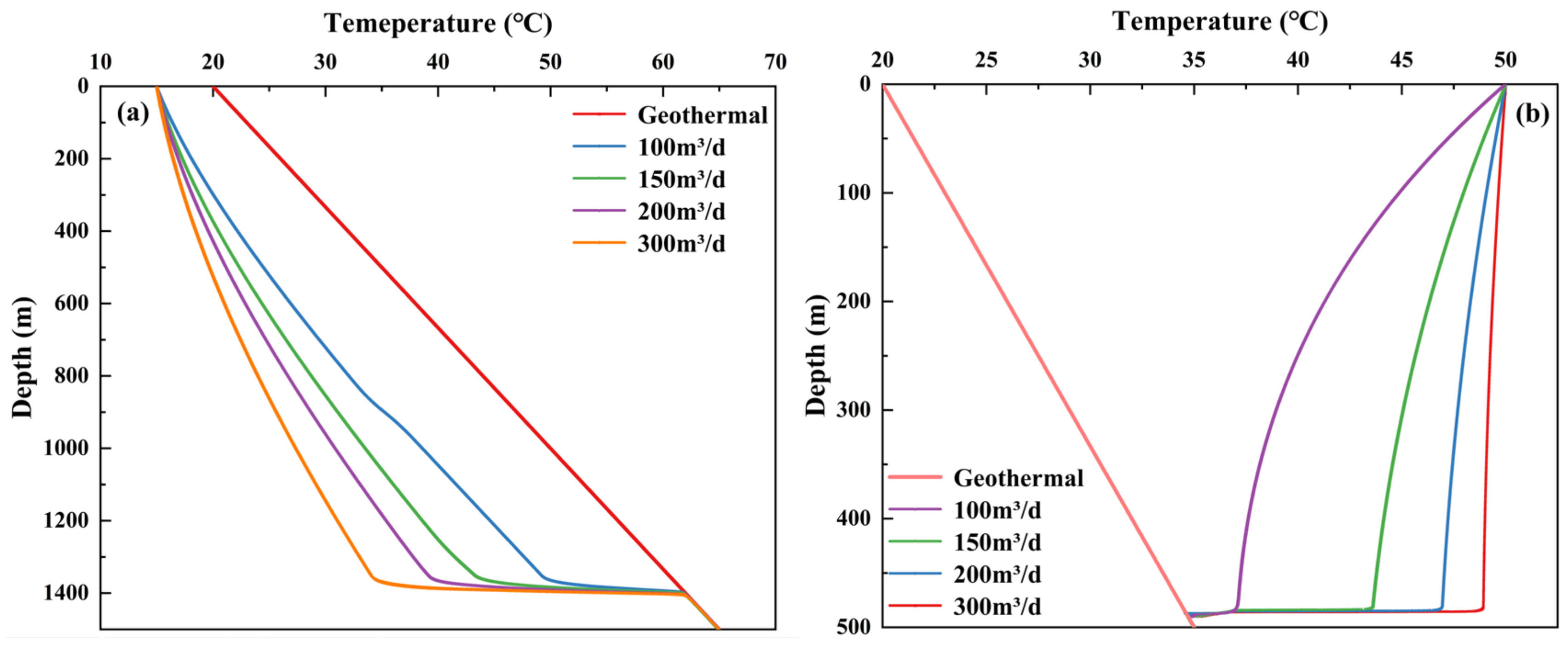
3.3.1. Injection Flow Rate

Under the influence of different work systems, the total injection flow rate of the wellbore may vary. The total injection flow rate directly affects the heat exchange process between the injected water and the reservoir fluid and rock, and it can reflect the distribution pattern of injected water in the reservoir. To investigate the effect of total injection flow rate on wellbore temperature, considering the influence of a water absorbing layer, this paper analyzes the impact of different injection flow rates on wellbore temperature changes under injection temperatures of 20 °C and 50 °C, respectively. We specifically analyzed the temperature changes in the wellbore when the total injection volume was 100 m³·d⁻¹, 150 m³·d⁻¹, 200 m³·d⁻¹, and 300 m³·d, and presented relevant calculation results.

As shown in Figure 6, when the injection volume is 300 m³/d, the wellbore temperature reaches 34.7 °C at 1375 m, and when the injection volume is 100 m³/d, the wellbore temperature reaches 49.7 °C at the same position. As the injection flow rate decreases, the variation range of the wellbore temperature increases. This is because the higher injection rate accelerates the fluid velocity in the wellbore, reducing the time it takes the fluid to travel from the wellhead to the suction layer. The heat transfer time between the fluid and the surrounding formation is reduced, resulting in insufficient heat transfer between the formation and the fluid. Therefore, the temperature change range is reduced. The influence of the formation heat flux and temperature gradient is reduced by a higher water injection flow. In addition, at the main suction layer, the wellbore temperature changes dramatically and rapidly approaches the formation temperature, eventually matching the geothermal gradient.

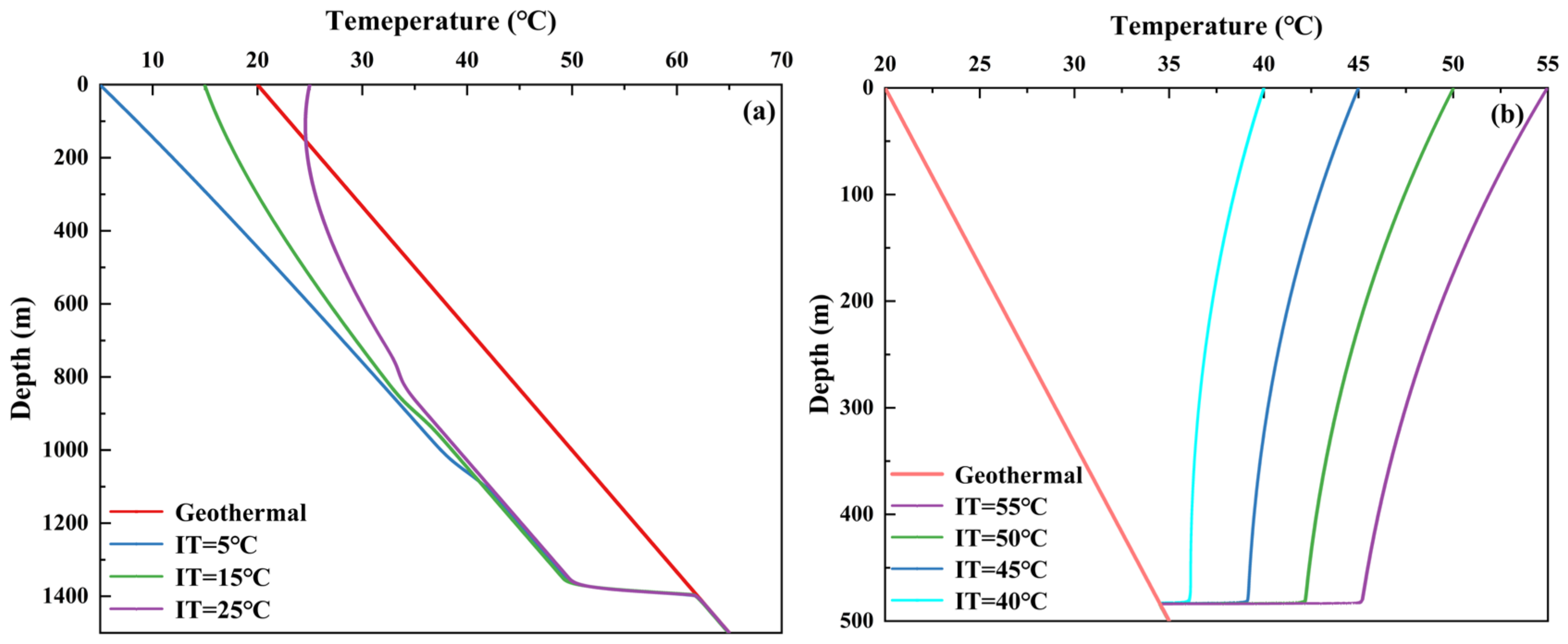
3.3.2. Injection Temperature

Figure 7 shows the wellbore temperature curve at different injection temperatures. The change in injection temperature is one of the very important parameters in the inversion model, especially in injection profile inversion based on temperature distribution. The change in injection temperature will directly affect the accuracy of the inversion model. Assuming the presence of a water absorbing layer, the injection temperatures set are 15 °C, 20 °C, 25 °C, 30 °C, 40 °C, 45 °C, 50 °C, and 55 °C, with IT being the injection temperature. Under the same injection flow rate conditions, when the injection temperature is higher than the formation temperature, the wellbore temperature will initially show a downward trend; however, when the temperature of the injected fluid intersects with the wellbore temperature, the trend of wellbore temperature change will shift from decreasing to increasing. The temperature of the wellbore will eventually approach the formation temperature and form a parallel line with the formation temperature. The greater the difference between the injection temperature and the formation temperature, the greater the amplitude of the wellbore temperature change, and it will gradually approach the formation temperature.

4. Interpretive Model and Field Application

4.1. Interpretive Model

4.1.1. Injection Profile Inversion Interpretation Model

When establishing an inversion interpretation model, the first step is to establish an objective function to characterize the error between the forward simulated temperature profile and the measured temperature profile. The objective function established in this study is the least squares function, where T_C represents the calculated value and TDTS represents the measured DTS temperature value, satisfying the following:

$$f\left(\mathrm{x}\right)=\omega {(T_c-T_{DTS})}^T(T_c-T_{DTS})$$

(12)

where $x$—flow profile distributed along the wellbore;

• $\omega$—temperature weight.

Therefore, the inversion of the injection profile model is to continuously change the flow rate distribution along the wellbore under stable injection so that the objective function satisfies the following conditions:

$$f\left(\mathrm{x}\right)<\epsilon$$

(13)

where $\epsilon$ is the acceptable accuracy error.

Inversion is a continuous iterative process and the objective function only determines the termination conditions of the inversion process. However, it is necessary to gradually reduce the objective function and approach an acceptable error accuracy as the inversion progresses.

4.1.2. Intelligent Optimization Algorithm Based on LSO-MCMC

Having established the above model, we need inversion methods to perform inversion calculations on the model to determine how to change the flow rate x so that the objective function converges to an acceptable range. The gradient-based inversion algorithm is a non-heuristic method which can gradually optimize the parameters in the model and is suitable for relatively simple inversion models. The inversion method based on the stochastic algorithm can search the optimal solution globally in the global space, and can approach the optimal solution quickly, which is suitable for more complex inversion models. DTS logging data have strong continuity and large-scale data volume characteristics. Based on the above considerations, this study selected the Markov chain Monte Carlo (MCMC) and Levenberg–Marquart (L-M) algorithms, representing stochastic-based and gradient-based inversion methods, respectively, and compared and analyzed the effects of different types of algorithms in practical inversion applications.

• Markov Chain Monte Carlo

The Markov chain Monte Carlo (MCMC) algorithm consists of the Monte Carlo method and a Markov chain. The basic idea is to use the Metropolis sampling method to construct a traversal Markov chain. Starting from any probability vector, through multiple iterations of calculation an invariant distribution is obtained which becomes the required sampling distribution. The larger the sampling frequency, the more stable the sampling distribution tends to be. MCMC sampling is based on Bayesian theory, and its expression is as follows:

$$\pi ({\theta }_i|y)={\displaystyle \frac{F(y|{\theta }_i)\pi ({\theta }_i)}{{\displaystyle \int F(y|\theta )\pi (\theta )d\theta }}}$$

(14)

where $\pi \left({\theta }_i\right)$—probability of basic parameter value being $\left({\theta }_i\right)$;

• $F(y|{\theta }_i)$—when the parameter value is $\left({\theta }_i\right)$, invert the probability density of parameter y;
• $\pi ({\theta }_i|y)$—probability of basic parameter value being $\left({\theta }_i\right)$.

2.

Light Spectrum Optimizer

Light Spectrum Optimizer (LSO) is a global optimization algorithm that seeks the optimal solution through an iterative process. However, the particle swarm optimization algorithm is essentially a stochastic algorithm, and even with the same parameters, the results obtained from each solution may be different.

To avoid the algorithm becoming stuck in local optima and to improve computational efficiency, (To prevent the algorithm from becoming trapped in local optima and to enhance computational efficiency,) the LSO (Abdel-Basset et al., 2022) algorithm introduces exploration and development mechanisms to achieve the search for global optima [23]. The optimization process initialization equation of the LSO algorithm can be expressed as the following:

$$\overrightarrow{x^o}=lb+R{V}_1(ub-lb)$$

(15)

where $\overrightarrow{x^o}$—the initial solution;

• $R{V}_1$—uniform random numbers generated;
• $lb$—the lower bounds of the search space;
• $ub$—the upper bounds of the search space.

The exploration mechanism of the LSO algorithm simulates the formation process of a rainbow, randomly selects solutions, and uses adaptive control factors to explore the search space. The development mechanism simulates the scattering process of light and uses probability control to adjust the search direction. The LSO algorithm adopts three scattering mechanisms, two of which focus on development, while the third mechanism enhances exploration by randomly selecting solutions. Therefore, the LSO algorithm can adaptively select the development or exploration mechanism based on the difference between the current solution and the optimal solution, thereby achieving a balance between exploration and development. Figure 8 shows the optimization process of the LSO algorithm.

3.

LSO-MCMC Intelligent Optimization Algorithm

The LSO-MCMC algorithm effectively integrates the randomness of spectral optimization algorithms, avoiding the risk of being trapped in local optima. At the same time, it inherits the efficiency of the Markov chain Monte Carlo (MCMC) algorithm, ensuring the prevention of dead loops. This hybrid algorithm offers advantages such as fast convergence, low computational complexity, and simplicity. In this study, an improved combined optimization algorithm, LSO-MCMC, is employed for inversion interpretation of injection profiles. The LSO algorithm is first used to perform a global search for a relatively optimal solution, which is then set as the initial value and input into the MCMC algorithm for further iterative calculations.

4.1.3. Optimization of Inversion Algorithm

In order to obtain the optimal inversion solution, this paper conducted selective research on inversion algorithms. Based on the forward temperature, the Markov chain Monte Carlo algorithm (MCMC) and the Levenberg–Marquardt algorithm (L–M) were used to invert the model. Figure 9 shows the well temperature curves obtained from the inversion of X well using the MCMC and L-M algorithms, respectively. It can be seen that the fitting effect of both algorithms is good at 3100–3300 m, while the MCMC algorithm performs significantly better than the L-M algorithm at 3300–3550 m.

Table 2. Comparison of LM algorithm and MCMC algorithm inversion.

Inverse Parameters	MCMC	LM
Iteration	1089	1273
Iterate (s)	89.01	117.63

shows the comparison of inversion results between the LM algorithm and MCMC algorithm. Under the same convergence conditions and optimization times, the MCMC algorithm has fewer average iterations and shorter iteration times compared to the L-M algorithm, and the inverted temperature is closer to the measured temperature curve. Therefore, considering all factors, the inversion performance of the MCMC algorithm is slightly better than that of the L-M algorithm, and the MCMC algorithm is chosen for inversion interpretation and evaluation.

For the inversion process, computational efficiency can be improved in the following four aspects. Metropolis–Hastings (MH) is a sampling method in MCMC. It constructs a proposal distribution that is easy to sample and generates samples of the target distribution through acceptance or rejection, quickly approaching the true value.

For the inversion process, an appropriate proposed distribution is chosen to optimize sampling efficiency. In the construction of forward modeling, the use of adjustable non-uniform grids, wellbore dense grids, and reservoir sparse grids can not only improve the calculation accuracy of wellbore temperature, but also significantly reduce the calculation time of coupled temperature prediction models.

The formation temperature is an important input parameter in the temperature model, and it can also be used to calculate the initial temperature of the wellbore through the wellbore trajectory. In the early stages of production, as the formation temperature has not yet returned to its original state, using the temperature during the DTS shut in period as the formation temperature during temperature inversion of on-site measured wells can significantly improve the calculation efficiency and fitting degree of inversion.

The selection of initial values for inversion has a significant impact on the inversion effect and speed. If the given initial value differs significantly from the true value, the inversion algorithm may only be able to find a local optimal solution, or even fall into a dead loop, resulting in lower accuracy or incorrect results. Therefore, an optimization algorithm is needed to ensure that a good initial value can be obtained at the beginning of the inversion. Based on the above considerations, the spectral optimization algorithm was combined with the Markov chain Monte Carlo algorithm to form the LSO-MCMC intelligent optimization method. Its high efficiency, flexibility, and ease of implementation make it an ideal choice for solving complex inversion problems. The process of injecting profile inversion interpretation is shown in the figure. (The inversion interpretation process of injection profile is shown in Figure 10.)

Figure 11 shows the temperature curves obtained by inversion using the MCMC and LSO-MCMC algorithms. It can be seen that both the MCMC and LSO-MCMC algorithms have a high degree of fitting in the non-water absorbing layer. However, in the water absorbing layer, the fitting effect of the LSO-MCMC algorithm is significantly better than that of the MCMC algorithm, and the iteration speed and convergence time of the LSO-MCMC algorithm are both better. Based on the above considerations, the LSO-MCMC intelligent optimization algorithm is used to invert, interpret, and evaluate the injection profile.

4.2. Field Application

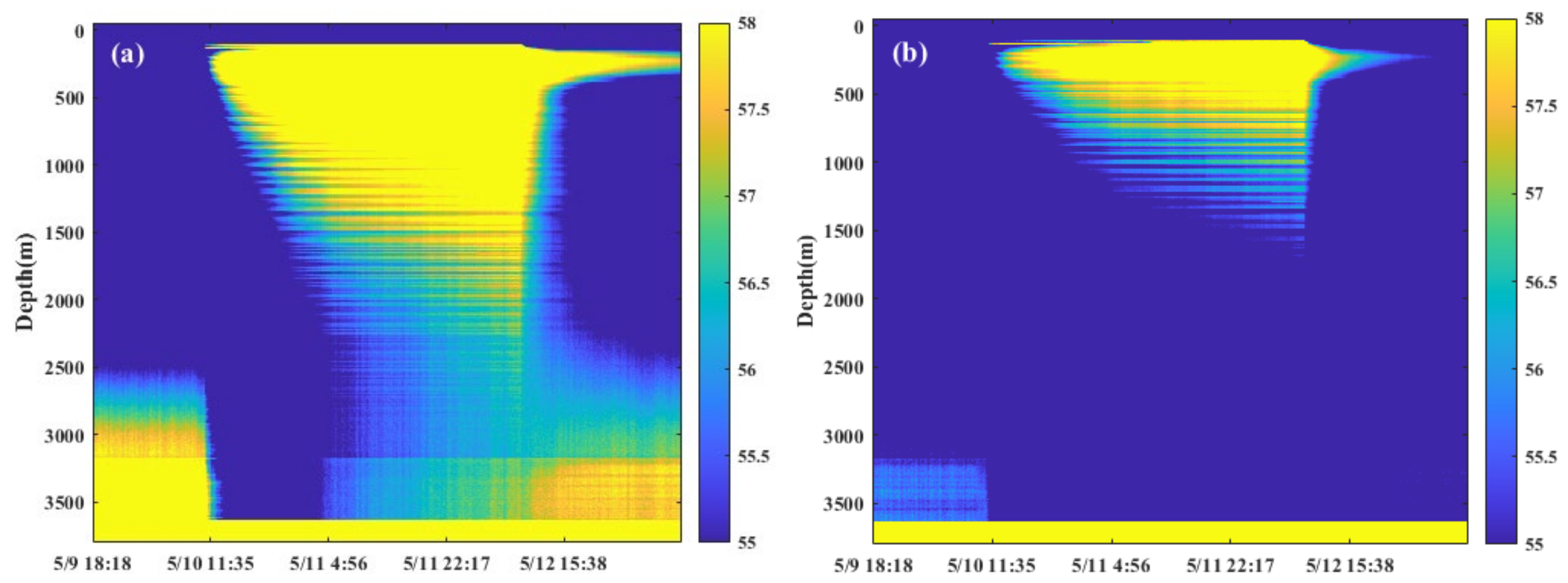
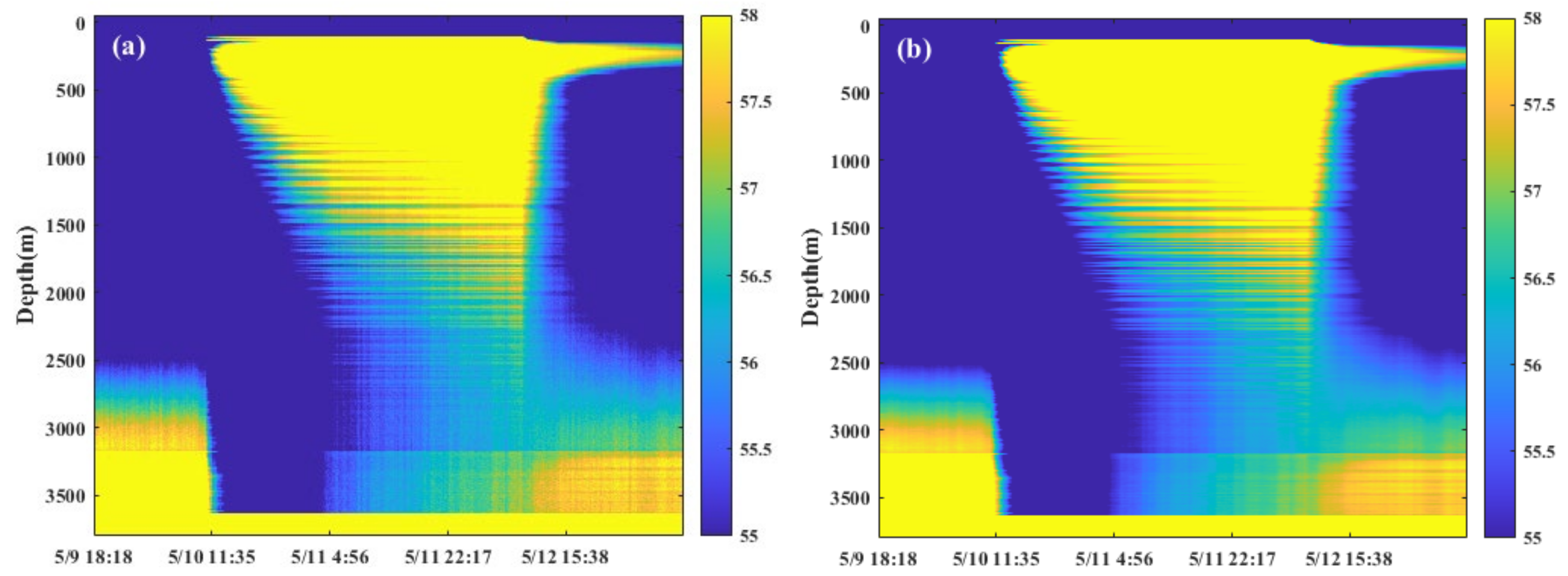
4.2.1. DTS Data Analysis

DTS data are usually affected by various noise sources, and fiber optic installation can cause system errors, temperature fluctuations, and affect data processing and analysis. Wavelet transform effectively separates noise and signals by decomposing signals into different frequency components and processing them simultaneously in both time and frequency domains. It is particularly suitable for signals with local abrupt changes or non-stationary characteristics. The continuous form of wavelet transform can be represented by the following convolution integral:

$$W(a,b)={\displaystyle {\int }_{-\infty }^{\infty }f(t)\cdot {\phi }^{\ast }(\frac{t-b}{a})}dt$$

(16)

This article studies two commonly used threshold denoising methods, soft thresholding and hard thresholding. Hard thresholding cannot achieve good denoising effects, while hard thresholding also causes signal distortion while removing noise. Figure 12 shows the imaging images before and after wavelet transform soft threshold filtering. DTS eliminates the noise signal after wavelet transform, but there is also distortion, which affects the inversion interpretation effect. Higher order wavelet basis functions can be used to improve reconstruction accuracy, or adaptive threshold denoising methods can be employed to preserve key signal features.

The Kalman filter is a recursive algorithm suitable for the state estimation of dynamic systems which can effectively process time series data and is particularly suitable for dynamically changing temperature data. Figure 13 shows the flowchart of the Kalman filter. This filtering method will predict and correct the entire system, continuously iterating to refine the process. During each iteration cycle, the method integrates measurement and prediction, thereby reducing the impact of noise on the data while preserving the original signal characteristics to the greatest extent possible.

Using Kalman filtering to process DTS logging data, Figure 14 shows the imaging images of DTS data before and after Kalman filtering. It can be seen that the DTS logging data appear clearer and smoother after filtering, retaining the key features of the original signal while filtering out noise signals. Moreover, the reading and processing speed of the filtered DTS data are significantly improved. Kalman filtering not only improves data quality but also enhances the efficiency and accuracy of data analysis.

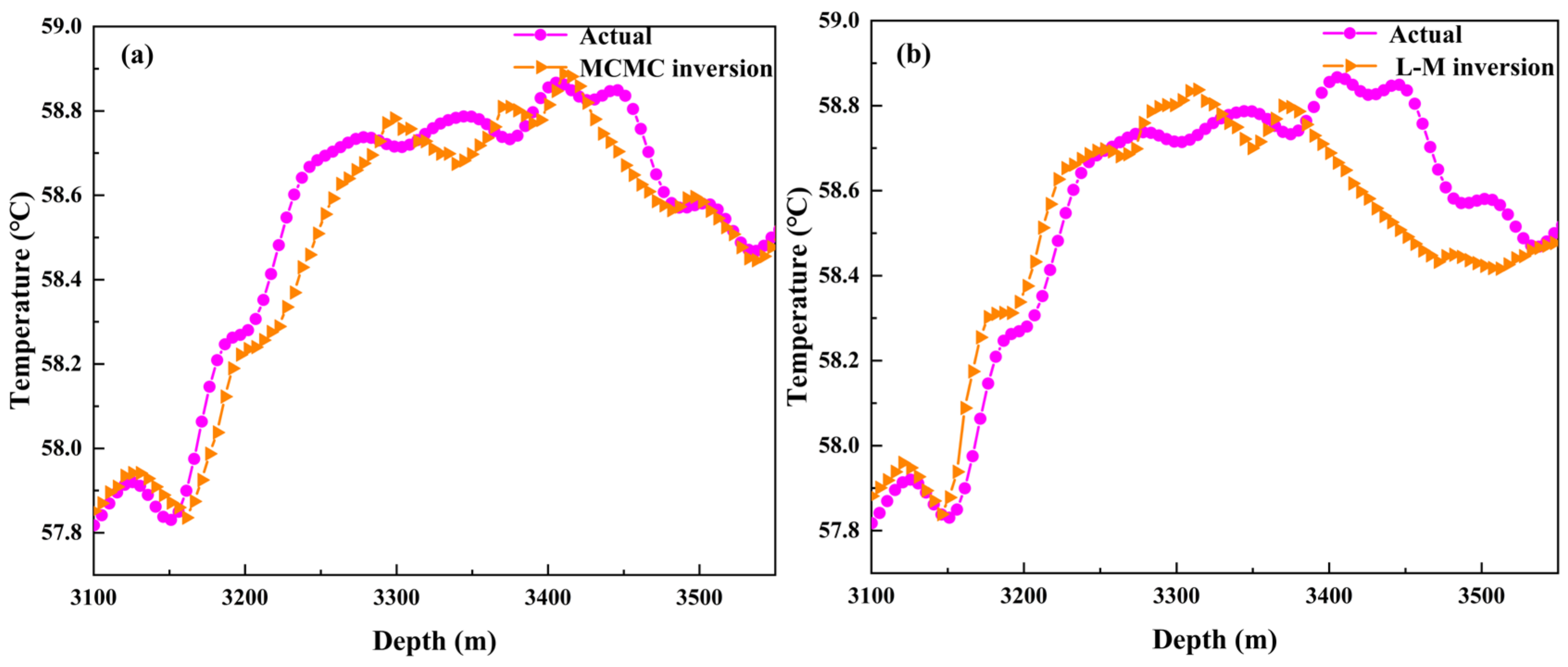
4.2.2. Injection Profile Inversion Interpretation and Evaluation

The inversion workflow is applied to a field case. X well is a horizontal water injection well, with a vertical depth of 1426.75 m and a length of 398.2 m in the horizontal section. The total depth of the well completion is 3572 m, the elevation of the core filling is 33.58 m, and the maximum wellbore inclination angle is 91.26°. The well is completed using an open hole completion method. During well completion, the pipe string is inserted and located 20.24 m below the top packer. The wellhead pressure is 6.8 MPa, the casing pressure is 3.1 MPa, and the pressure gradient is 0.90 MPa/100 m. The well resumed water injection from 10:30 on 10 May and stopped injection at 9:10 on 12 May. During this period, the daily injection volume reached 543 m³ and the daily allocation was 540 m³. Therefore, the DTS data at 10:30 on 10 May can be regarded as the temperature data of the reservoir after warming up. Figure 15 shows the interpretation results of the DTS injection profile in well X.

As shown in Figure 15, the first line in the figure is the depth line, (As shown in Figure 15, the first line in the figure is the depth trackthe) second line is the wellbore trajectory, the third line is the natural gamma curve, the fourth and fifth lines are the DTS two-dimensional imaging map and DTS temperature difference imaging map, the sixth line is the formation temperature curve and DTS measured curve, the seventh line is the pipe structure, the eighth line is the borehole position, and the ninth and tenth lines are the interpretation result lines. From the figure, it can be seen that the measured temperature curve of DTS is significantly higher than the formation temperature. This is because the injection temperature of the well is 58 °C, which is higher than the formation temperature. After injecting water for a period of time, the temperature of the heat transfer wellbore increases significantly. Here, we adopted the LSO-MCMC combination algorithm and took the temperature data at 10:30 on 10 May, that is, the temperature during the shut in period, as the formation temperature for the inversion calculation of well X. The meshing is performed in an uneven way, with an ultra-tight mesh of 0.001 m near the wellbore and a tight mesh of 0.5 m away from the wellbore.

At 3100 m to 3300 m, the two curves basically coincide. In the main water absorption layer, due to the complex flow relationship between the fluid in the wellbore and the reservoir, there is a slight deviation between the inverted temperature at 3300 m to 3550 m and the measured temperature. However, the temperature changes in the two are basically consistent, and the inverted flow profile can meet the practical application requirements.

Table 3. Comparison between PLT interpretation results and inversion results.

Oblique Depth (m)	Thickness (m)	PLT-Aiv (m3/d)	PLT-Riv (%)	Inversion-Aiv (m3/d)	Inversion-Riv (%)
3202.7–3214.3	11.6	24.9	4.6	25.2	5.0
3279.2–3293.4	14.2	29.7	5.5	30.2	5.6
3354.2–3367.1	12.9	27.0	5.0	30.7	5.7
3372.0–3383.4	11.4	23.9	4.4	26.6	4.6
3396.4–3404.0	7.6	15.9	2.9	19.4	3.6
3420.5–3452.0	31.5	65.8	12.2	51.8	9.6
3463.7–3469.1	5.4	11.1	2.1	9.7	1.8
3475.7–3484.6	8.9	18.6	3.4	16.4	3.0
3494.5–3513.3	18.8	39.2	7.3	36.3	6.7
3536.7–3540.2	23.5	35.5	6.6	31.4	5.8
3540.2–3552.0	11.8	248.4	46.0	262.3	48.5
Amount to (Sum total)		540.0	100.0	540.0	100.0

shows the comparison between the PLT interpretation results and the inverted flow profile, where Aiv is the absolute inhalation volume and Riv is the relative inhalation volume. The PLT interpretation results show that the section from 3300 m to 3552 m is the water absorbing layer, while the section from 3540 m to 3552 m is the main water absorbing layer, with an absolute water absorption of 248.4 m³/d and a relative water absorption of 46%. The inversion results show that the main water absorbing layer is from 3540 m to 3552 m, with an absolute water absorption of 262.3 m³/d and a relative water absorption of 48.5%. By comparing the inversion results with the PLT interpretation results, it can be seen that in the 3100 m to 3300 m range, the two are relatively consistent. In the section from 3300 m to 3572 m, there are some differences in the interpretation results, but the identification of the main water absorbing layer is more accurate and can meet the practical application needs.

5. Conclusions

(1)

This study established a flow and thermal model for the wellbore and reservoir, which were coupled through appropriate boundary conditions to form a coupled temperature prediction model for single-phase flow which solved iteratively based on the finite difference method. (The flow and thermal models of wellbore and reservoir are established, coupled by appropriate boundary conditions, and a single-phase flow coupling temperature prediction model is formed. The model is iteratively solved based on the finite difference method. This method is suitable for the thermal model with simple downhole heat transfer, and has the advantages of high computational efficiency, high flexibility and simple realization.)

(2)

In this study, the results of the finite difference calculation are compared with those of the numerical simulation to verify the reliability of the finite difference method. In addition, the influence of fluid properties on the transient wellbore temperature distribution is also studied. The results show that injection velocity and injection temperature have different effects on the transient temperature curve, and the injection amount is negatively correlated with the change rate of the transient temperature curve, which provides a theoretical basis for determining the inflow rate by using the transient temperature data. In addition, an inverse model is established on the basis of the forward model to identify the change in downhole fluid flow and pinpoint the main suction layer by using the measured temperature data.

(3)

Based on the characteristics of DTS data, the inversion interpretation model has been optimized in the following four aspects: inversion algorithm, model grid, initial parameters, and inversion process, which can quickly and accurately approximate the measured temperature.

(4)

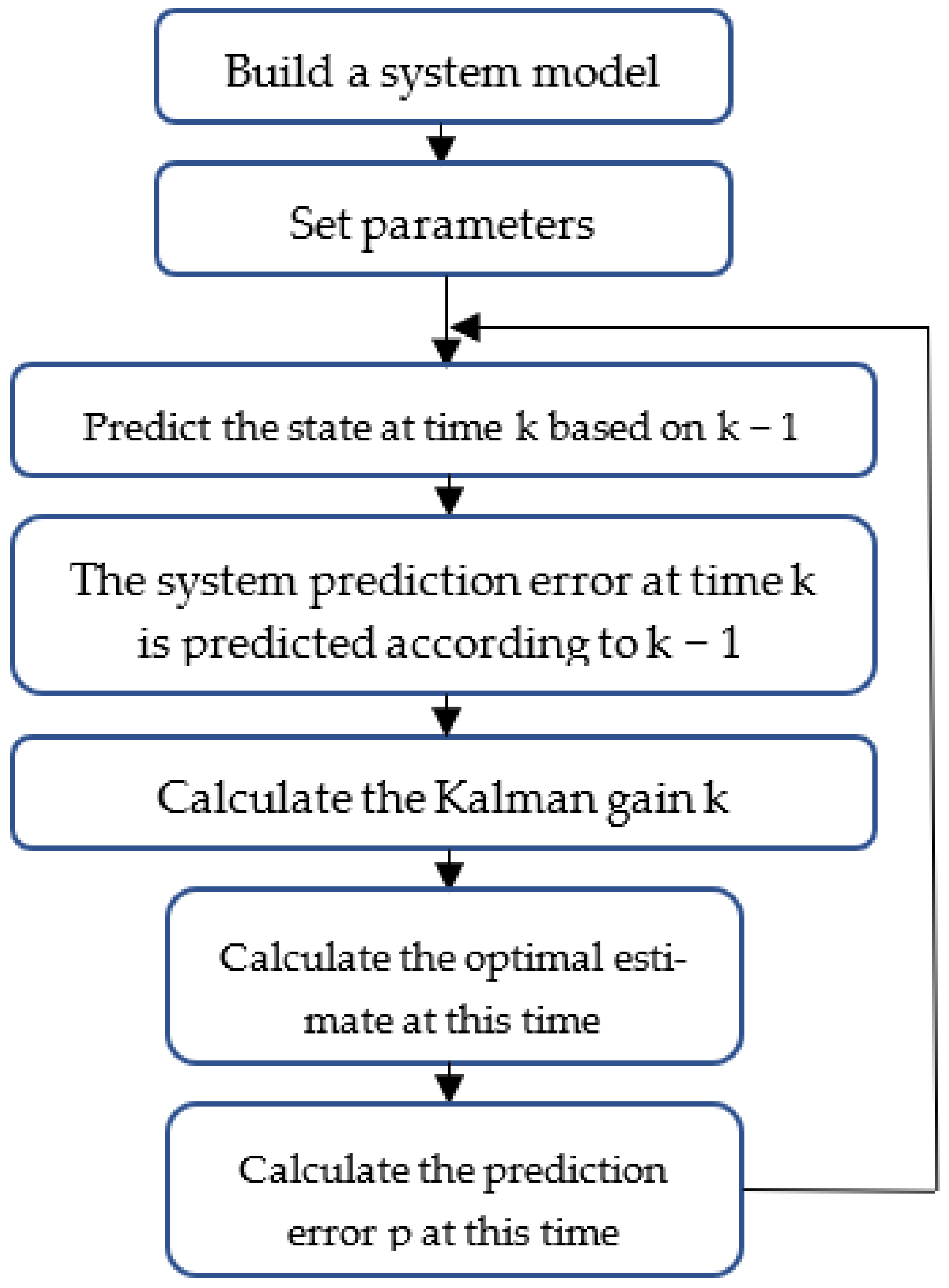
The results indicate that noise significantly impacts the speed of data compilation and the accuracy of logging interpretation. In scenarios with high signal-to-noise ratios (SNR), the Kalman filter not only enhances interpretation precision but also accelerates data unmarshaling, while simultaneously mitigating potential data distortion caused by filtering. Based on the LSO-MCMC combination optimization algorithm, the inversion interpretation and evaluation of X injection well were carried out and the inverted flow profile can meet the practical application requirements.

References

1. Dai, C.; Zhang, Y. Application of distributed temperature sensing in wellbore monitoring: Numerical simulation and field analysis. J. Pet. Sci. Eng. 2015, 135, 423–437. [Google Scholar]
2. Hasan, A.R.; Kabir, C.S. Aspects of heat transfer during two-phase flow in wellbores. SPEPF 1994, 9, 211–216. [Google Scholar] [CrossRef]
3. Hasan, A.R.; Kabir, C.S. Fluid Flow and Heat Transfer in Wellbores; Society of Petroleum Engineers: Richardson, TX, USA, 2002. [Google Scholar]
4. Yoshioka, K. Detection of water or gas entry into horizontal wells by using permanent downhole monitoring systems. Ph.D. Thesis, Texas A&M University, College Station, TX, USA, 2007. [Google Scholar]
5. Sui, W.; Zhu, D. Determining multilayer formation properties from transient temperature and pressure measurements in gas wells with commingled zones. J. Nat. Gas Sci. Eng. 2012, 9, 60–72. [Google Scholar] [CrossRef]
6. Hasan, A.R.; Izgec, B.U.L.E.N.T.; Kabir, C.S. Sustaining Production by Managing Annular-Pressure Buildup. SPE Prod. Oper. 2010, 25, 195–203. [Google Scholar] [CrossRef]
7. Li, Z.; Zhu, D. Predicting flow profile of horizontal well by downhole pressure and distributed-temperature data for waterdrive reservoir. SPE Prod. Oper. 2010, 25, 296–304. [Google Scholar] [CrossRef]
8. Yoshida, N. Modeling and Interpretation of Downhole Temperature in a Horizontal Well with Multiple Fractures. Ph.D. Thesis, The University of Tokyo, Tokyo, Japan, 2016. [Google Scholar]
9. Shiyan, Z. Theoretical Study on Interpretation of Horizontal Well Production Profile Based on Distributed Fiber Optic Temperature Testing. Master’s Thesis, Southwest Petroleum University, Chengdu, China, 2016. [Google Scholar]
10. Chen, L.; Yu, Z. Establishment and application of wellbore temperature and pressure model of unsteady flow in gas Wells. Nat. Gas Ind. 2017, 37, 70–76. [Google Scholar]
11. Huang, L.; Song, H.W.; Wang, M.X.; Ma, W.H.; Wei, B.J. Injection and Production Profile Interpretation Method Based on Distributed Fiber Optic Temperature Logging. Prog. Geophys. 2024, 39, 266–279. [Google Scholar]
12. Luo, H.; Li, H.; Li, Y.; Wang, F.; Xiang, Y.; Jiang, B.; Yu, H. Inversion and interpretation of production profile and fracture parameters of fractured horizontal wells in low-permeability gas reservoirs. Acta Pet. Sin. 2021, 42, 936. [Google Scholar]
13. Junjun, C. Research on Prediction and Interpretation Model of Horizontal Well Borehole Temperature. Master’s Thesis, Southwest Petroleum University, Chengdu, China, 2016. [Google Scholar]
14. Smith, J.; Zhang, Y. A three-dimensional transient multiphase flow model for box-shaped reservoirs. J. Pet. Sci. Eng. 2023, 213, 123456. [Google Scholar]
15. Wang, X.; Li, J. Numerical simulation of injection wells: A forward model for pressure and temperature analysis. J. Pet. Technol. Sci. 2022, 15, 345–359. [Google Scholar]
16. Luo, H.; Li, H.; Jiang, B.; Li, Y.; Lu, Y. A new method for interpreting the production profile of fractured horizontal wells in low-permeability gas reservoirs based on DTS data inversion. Nat. Gas Geosci. 2019, 30, 1639–1645. [Google Scholar]
17. Lin, J. Proceedings of the International Field Exploration and Development Conference 2019; Springer Science and Business Media LLC: Singapore, 2020. [Google Scholar]
18. Li, H.; Luo, H.; Xiang, Y.; Li, Y.; Jiang, B.; Cui, X.; Gao, S.; Zou, S.; Xin, Y. DTS based hydraulic fracture identification and production profile interpretation method for horizontal shale gas wells. Nat. Gas Ind. B 2021, 8, 494–504. [Google Scholar] [CrossRef]
19. Wei, C.; Mao, L.; Yao, C.; Yu, G. Heat transfer investigation between wellbore and formation in U-shaped geothermal wells with long horizontal section. Renew. Energy 2022, 195, 972–989. [Google Scholar] [CrossRef]
20. Yoshida, N.; Zhu, D.; Hill, A.D.D. Temperature-Prediction Model for a Horizontal Well with Multiple Fractures in a Shale Reservoir. SPE Prod. Oper. 2014, 29, 261–273. [Google Scholar] [CrossRef]
21. Kim, J.; Cho, M.-K.; Jung, M.; Kim, J.; Yoon, Y.-S. Rotary hearth furnace for steel solid waste recycling: Mathematical modeling and surrogate-based optimization using industrial-scale yearly operational data. Chem. Eng. J. 2023, 464, 142619. [Google Scholar] [CrossRef]
22. Chung, I.; Kim, J.; An, J.; Lee, D.; Park, J.; Oh, H.; Yun, Y. Kinetic modeling of the oxidative dehydrogenation of propane with CO2 over a CrOx/SiO2 catalyst and assessment of CO2 utilization. Chem. Eng. J. 2024, 494, 153178. [Google Scholar] [CrossRef]
23. Abdel-Basset, M.; Mohamed, R.; Sallam, K.M.; Chakrabortty, R.K. Light Spectrum Optimizer: A Novel Physics-Inspired Metaheuristic Optimization Algorithm. Mathematics 2022, 10, 3466. [Google Scholar] [CrossRef]
Figure 1. Steps for solving the coupling model of multi-phase flow well and reservoir in production wells.
Processes 13 00733 g001
Figure 2. Reservoir fluid flow model.
Processes 13 00733 g002
Figure 3. Reservoir fluid temperature profile. (a) Different fluid types; (b) different wellbore radii and reservoir thicknesses.
Processes 13 00733 g003
Figure 4. Reservoir fluid temperature profile. (a) Different oil–water ratios; (b) different gas–water ratios.
Processes 13 00733 g004
Figure 5. Numerical simulation and finite difference calculation of well temperature curve (where (a,c) are finite difference calculation results; (b,d) are numerical simulation results).
Processes 13 00733 g005aProcesses 13 00733 g005b
Figure 6. Temperature curves of wellbore with different injection flow rates. (a) The injection temperature is 20 °C; (b) the injection temperature is 50 °C.
Processes 13 00733 g006
Figure 7. Temperature curves of wellbore with different injection temperature. (a) The injection temperatures are 5 °C, 15 °C, 25 °C; (b) the injection temperatures are 40 °C, 45 °C, 50 °C, 55 °C.
Processes 13 00733 g007
Figure 8. Flowchart of LSO.
Processes 13 00733 g008
Figure 9. Invert well temperature curve. (a) Is the MCMC algorithm; (b) is the L-M algorithm.
Processes 13 00733 g009
Figure 10. LSO-MCMC algorithm inversion interpretation process.
Processes 13 00733 g010
Figure 11. Inversion of well temperature curve: (a) Is the MCMC algorithm; (b) is the LSO-MCMC algorithm.
Processes 13 00733 g011
Figure 12. DTS logging data wavelet transform filtering: (a) is before filtering; (b) is after filtering.
Processes 13 00733 g012
Figure 13. Flow chart of Kalman filtering.
Processes 13 00733 g013
Figure 14. DTS logging data Kalman filtering: (a) is before filtering; (b) is after filtering.
Processes 13 00733 g014
Figure 15. DTS inversion interpretation result chart of X well.
Processes 13 00733 g015