Low-Carbon Economic Scheduling of Hydrogen-Integrated Energy Systems with Enhanced Bilateral Supply–Demand Response Considering Vehicle to Grid Under Power-to-Gas–Carbon Capture System Coupling

Abstract

Hydrogen-Integrated energy systems (HIESs) are pivotal in driving the transition to a low-carbon energy structure in China. This paper proposes a low-carbon economic scheduling strategy to improve the operational efficiency and reduce the carbon emissions of HIESs. The approach begins with the implementation of a stepwise carbon trading framework to limit the carbon output of the system. This is followed by the development of a joint operational model that combines hydrogen energy use and carbon capture. To improve the energy supply flexibility of HIESs, modifications to the conventional combined heat and power (CHP) unit are made by incorporating a waste heat boiler and an organic Rankine cycle. This results in a flexible CHP response model capable of adjusting both electricity and heat outputs. Furthermore, a comprehensive demand response model is designed to optimize the flexible capacities of electric and thermal loads, thereby enhancing demand-side responsiveness. The integration of electric vehicles (EVs) into the system is analyzed with respect to their energy consumption patterns and dispatch capabilities, which improves their potential for flexible scheduling and enables an optimized synergy between the demand-side flexibility and system operations. Finally, a low-carbon economic scheduling model for the HIES is developed with the objective of minimizing system costs. The results show that the proposed scheduling method effectively enhances the economy, low-carbon performance, and flexibility of HIES operation while promoting clean energy consumption, deep decarbonization of the system, and the synergistic complementarity of flexible supply–demand resources. In the broader context of expanding clean energy and growing EV adoption, this study demonstrates the potential of energy-saving, emission-reduction systems and vehicle-to-grid (V2G) strategies to contribute to the sustainable and green development of the energy sector.

1. Introduction

Currently, the conflict between economic and social development and environmental protection has become increasingly prominent due to severe energy depletion and the deteriorating ecological environment [1,2]. To address the energy and environmental crises, such as excessive carbon emissions caused by fossil fuel use, the Chinese government has proposed dual-carbon development targets [3]. The energy and power industry, as the main source of carbon emissions, is a key regulatory area for carbon emission reduction, with an urgent need to improve clean energy utilization efficiency and accelerate energy structure transformation [4,5]. To promote green and sustainable economic development, it is essential to leverage advanced communication technologies to aggregate renewable energy and efficient, clean hydrogen energy, while harnessing the synergies of energy technologies and the advantages of multi-energy complementarity [6,7]. It is also crucial to build an energy internet system with HIES as the emerging carrier [8]; maximizing the flexibility of scheduling resources across both supply and demand sectors will be crucial for improving the system efficiency and lowering carbon emissions [9].

Traditional energy storage technologies, which are stable, efficient, and economical, play a crucial role in the utilization of renewable energy and the adjustment of the energy structure. For example, redox flow batteries can stabilize the intermittent output of solar and wind energy, thereby increasing their share in power generation and facilitating their integration into the grid. However, these technologies are constrained by energy density and the larger physical space required for deployment, limiting their scalability in large-scale energy storage solutions. In contrast, hydrogen-based power-to-gas (P2G) technology offers higher energy density and greater long-term storage potential, enabling more effective long-term storage of renewable energy. This makes P2G particularly advantageous for stabilizing the grid and integrating large amounts of wind and solar renewable energy. Ref. [10] proposes an optimal operation strategy for integrated multi-energy systems incorporating P2G, significantly enhancing the system’s economic, environmental, and flexibility benefits. Ref. [11] achieves efficient energy sharing through the optimal planning of P2G and power units, thereby improving the system supply stability. Ref. [12] integrates P2G devices with flexible loads to reduce fluctuations between power supply and demand, thus improving the overall system efficiency. Refs. [13,14] develop an efficient operational framework for a P2G-integrated system utilizing stepwise carbon trading, aiming to attain the system’s environmental sustainability and low-carbon outcomes. The methanation process in P2G plants enables coupling with carbon capture systems (CCSs), thus facilitating systematic carbon recycling and reducing greenhouse gas emissions. Refs. [15,16] propose a low-carbon system operation strategy for the joint operation of P2G and CCS, enhancing the system’s low-carbon economic performance through ${\mathrm{CO}}_2$ capture and utilization. However, most P2G devices in existing P2G-CCS coupling studies are conventional models, necessitating further refinement of P2G’s two-stage operation to fully realize the potential of hydrogen energy utilization.

CHP has been widely adopted as an efficient energy supply mode in energy systems. However, its constant electro-thermal ratio output makes it difficult to meet the energy demands of variable loads. In response to this challenge, various thermoelectric decoupling methods have been proposed by scholars. Refs. [17,18] combine concentrating solar power with CHP units, thereby extending the operating range of the units through model coupling and reducing energy consumption, while promoting clean energy use. Ref. [19] introduces heat pumps into the CHP operational framework to enhance the overall system heating performance through the synergistic effect of the heat pump cycle, optimizing energy utilization under varying operating conditions. Ref. [20] couples a heat pump with a CHP unit to increase heat production by converting renewable resources, such as food waste, thus minimizing the adverse environmental effects of food waste. Although the above strategy extends the heating range of the unit, it fails to address excess heat generation. Therefore, refs. [21,22] introduce an Organic Rankine Cycle (ORC) in the CHP unit to convert part of the heat generation into electricity for supply, further optimizing the unit’s output. Although the methods proposed in the literature have improved the flexibility of the system energy supply to some extent, the complexity and variability of demand-side energy loads make it difficult for the supply side to unilaterally address excess heat or power generation. Additionally, these methods fail to fully utilize demand-side flexible resource regulation, limiting their impact on improving the system operational efficiency.

Integrated Demand Response (IDR), as a powerful means to stimulate the utilization of resources on the energy-using side, can mitigate the fluctuation between peak and off-peak loads and alleviate the supply–demand imbalance. It is also an effective measure to improve the clean energy consumption rate and low-carbon performance of HIESs. Ref. [23] develops a multivariate IDR model incorporating time-of-use pricing and incentive compensation mechanisms to realize the system’s low-carbon and economically efficient operation. Ref. 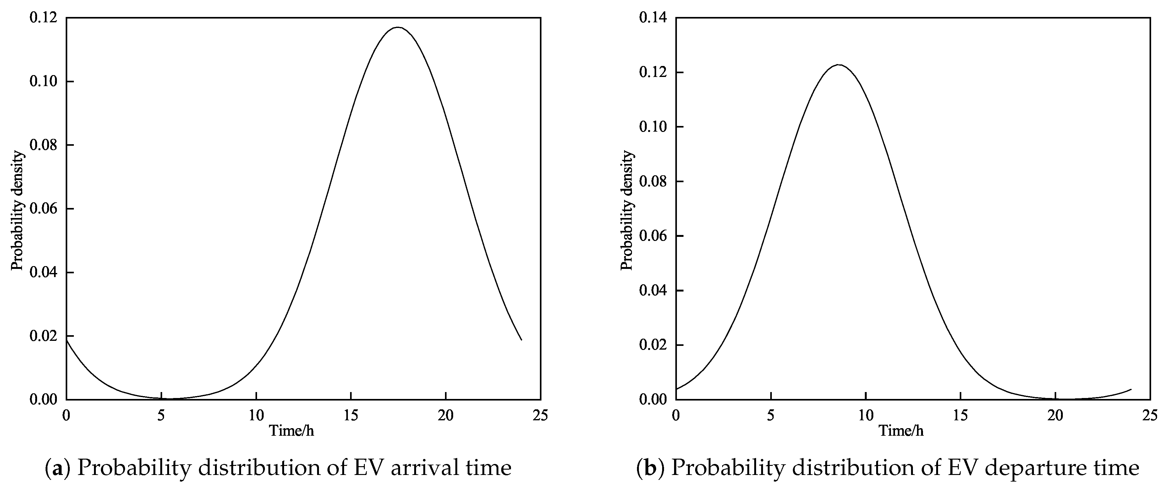[24] develops a refined IDR model that considers price elasticity and temperature-aware ambiguity, significantly improving the system’s low-carbon efficiency and economic performance. In addition to conventional loads, the dual load and storage attributes of EVs make them an ideal dispatch unit. Their potential for large-scale dispatch provides an effective means for the demand side’s contribution to the system’s optimal operation. Ref. [25] develops an EV charging demand model based on the behavioral characteristics of electric vehicles, and verifies its effectiveness for system optimization regarding carbon emissions and economic performance. Ref. [26] proposes time-of-use tariffs and nodal carbon potential-guided EV charging and discharging strategies, which have been shown to effectively reduce carbon emissions and operating costs in the system. Ref. [27] develops an EV charging and discharging strategy based on EV travel paths considering V2G, which satisfies the EV charging demand and optimizes the grid load profile. The above studies are all about the effect of demand-side flexible loads and EVs on system optimization when they act singly or together, and there is still a gap in the study of supply-side thermo-electrolytically coupled CHP units and demand-side load IDRs as well as V2Gs as the object of supply–demand synergistic optimization, which is yet to be further studied for its synergistic optimization benefits.

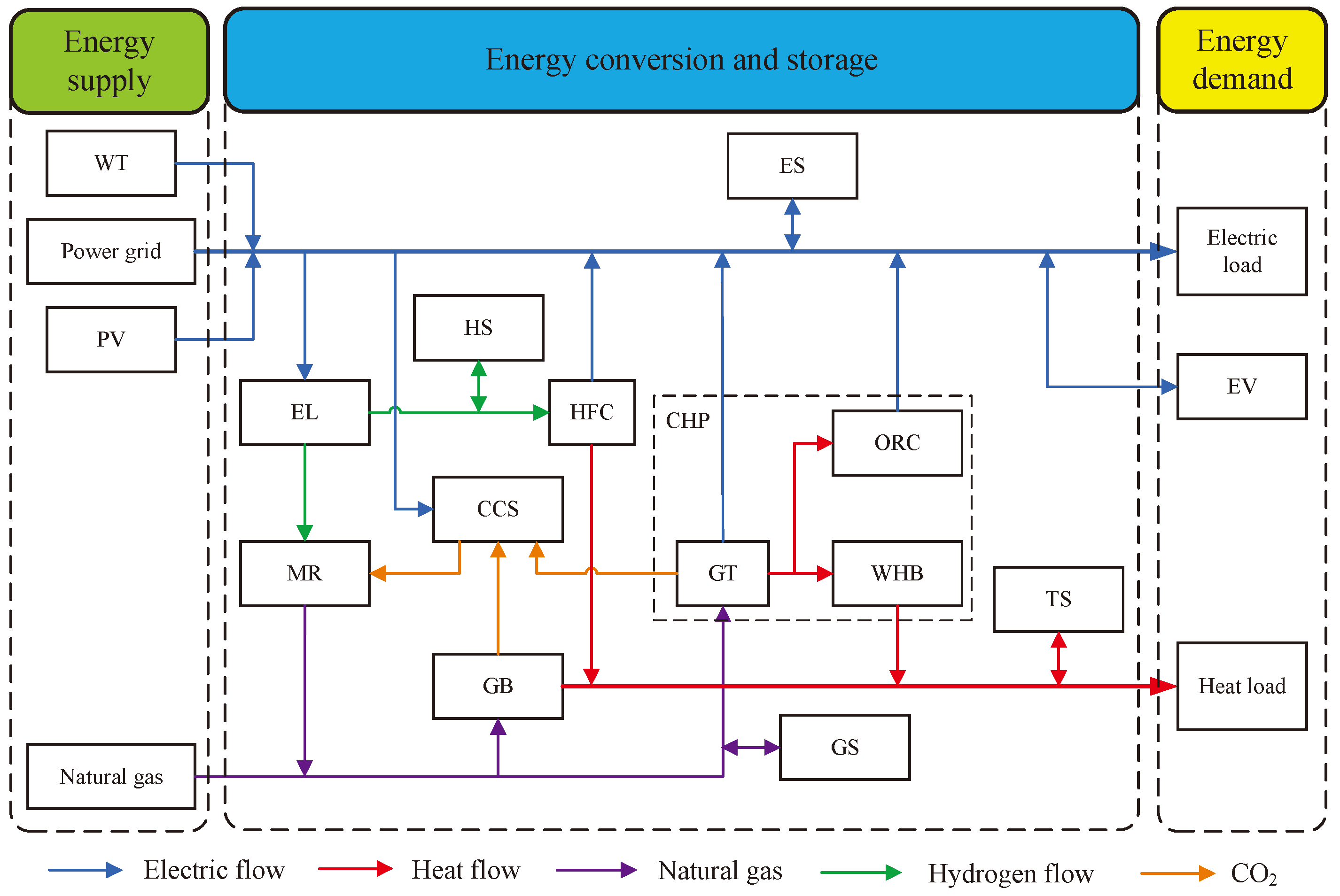
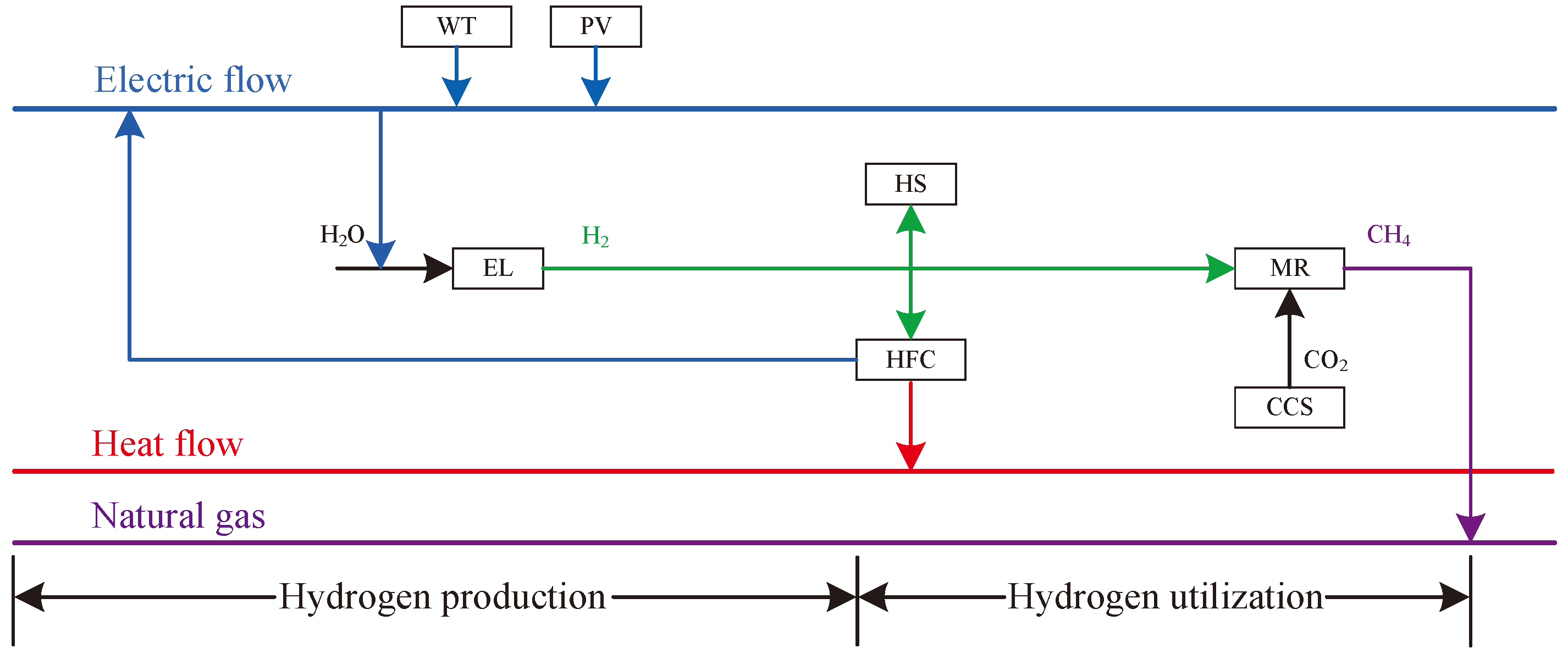
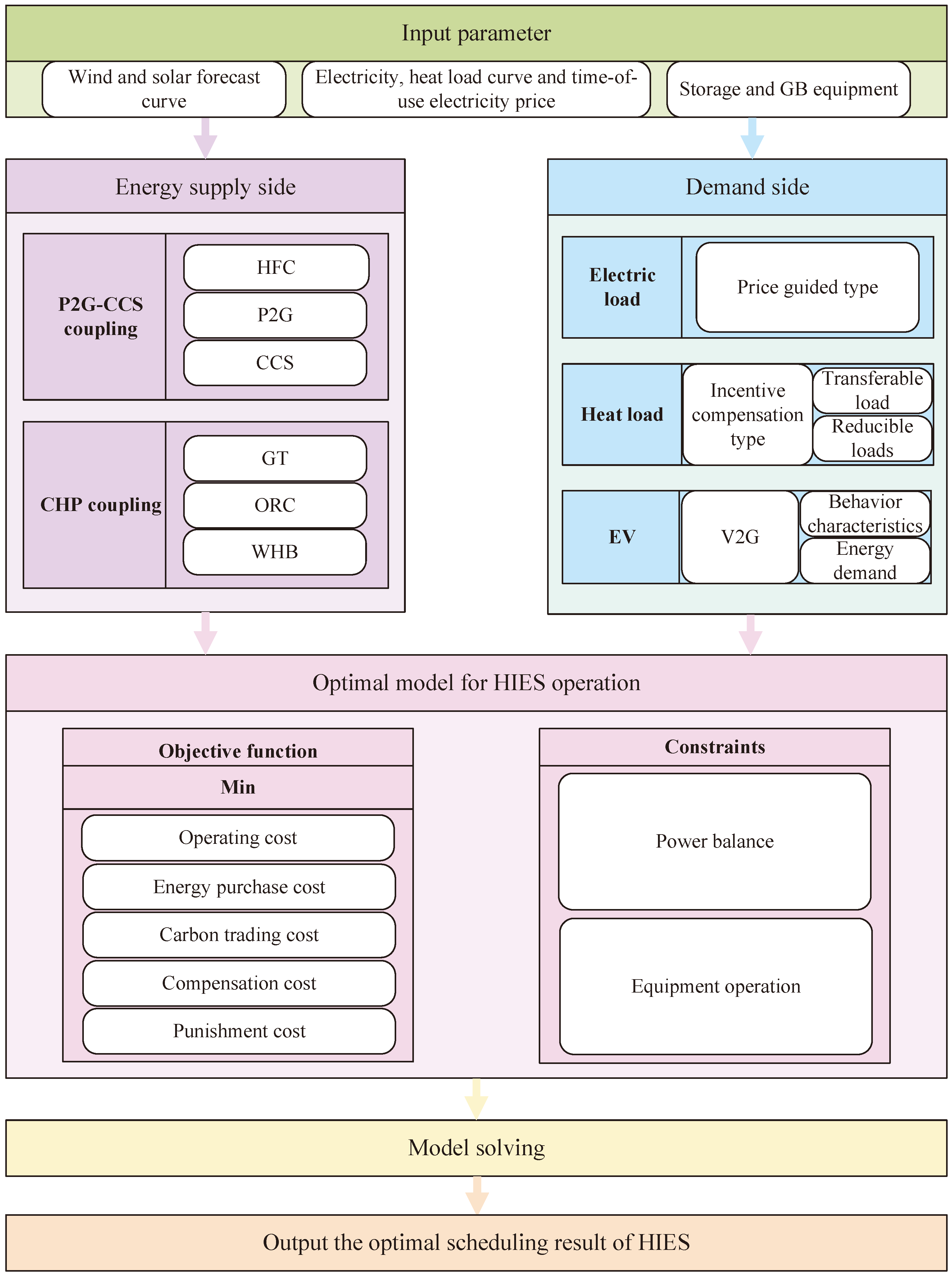
Building upon the aforementioned research context, this paper presents a low-carbon operational strategy for HIESs, taking into account the integrated P2G-CCS operation and the dual responsiveness of supply and demand. Firstly, a HIES operation framework with multiple energy forms that closely complement each other is proposed. A stepped carbon trading scheme is implemented to manage the carbon emissions generated by the system, alongside a refined coupling of CCS with two stages of P2G containing hydrogen fuel cells (HFCs), aimed at exploring the green path to promote the varied applications of hydrogen energy. Then, a CHP response model with flexible electricity and heat output is constructed using ORC and a waste heat boiler (WHB) on the energy supply side. The integrated response model, guided by tariffs and incentivized by compensation, is constructed on the demand side built upon the energy consumption patterns of electrical and thermal demands, respectively. Based on this, the V2G response model of EVs is constructed to enhance the system operational performance by facilitating the mutual interaction between supply and demand. Finally, a supply–demand co-optimization model for HIESs is developed with the goal of minimizing the overall system cost. The effectiveness of the proposed approach in improving both the low-carbon and economic performance of the system is demonstrated by comparing different scenarios.

The primary contributions of this research are outlined below:

(1) Constructing a coupled P2G-CCS operation model with HFCs in HIESs provides a new path for the utilization of wind and solar power, enabling the complete consumption of clean energy in the electricity generation sector. Simultaneously, it facilitates the integrated operation of the system’s electricity, heating, and gas networks through the synergy of multiple energy sources, with hydrogen acting as the connecting link, thus enhancing the system’s effective utilization of energy resources.

(2) The introduction of the ORC and WHBs on the energy supply side lifts the limitations of traditional CHP units’ thermoelectric coupling, effectively expanding the thermoelectric supply capacity. This improves the high efficiency and flexibility of the HIES’ energy supply. Together with the demand-side flexible electric and thermal loads, these advancements support the optimization of low-carbon and economic efficiency in HIESs.

(3) Based on the flexibility of demand-side load IDR characteristics, the V2G optimization of EV dispatchable resources is introduced to further enhance the demand side’s flexible regulation capability. This improves the stability and flexibility in the system performance, while ensuring the low-carbon and economic nature of HIESs.

2. Operational Framework for HIESs

The HIES operational framework presented in this paper is shown in Figure 1. The energy supply includes photovoltaic (PV) systems, wind turbine (WT) systems, the power grid, and the gas grid. Energy conversion encompasses CHP units, gas boilers (GBs), HFCs, and P2G devices, with the CHP units comprising gas turbines (GTs), WHBs, and ORC. The P2G systems include electrolysis tanks (ELs), methane reactors (MRs), and CCS units. Energy storage consists of electrical storage (ES), gas storage (GS), thermal storage (TS), and hydrogen storage (HS). Energy demand includes electricity, heat loads, and EVs.

2.1. Stepwise Carbon Trading Model

To encourage carbon emitters to actively reduce their emissions, the carbon trading mechanism grants carbon emission rights the attribute of freely tradable commodities, thereby constraining emitters to lower their emissions. In the event that the actual carbon emissions of the assessed entity surpass its allocated carbon allowances, the entity is required to acquire supplementary emission permits from the carbon market. Conversely, any surplus allowances can be sold for profit. The flowchart of the carbon trading principles is shown in Figure 2.

2.1.1. Carbon Allowance Allocation Modeling

The baseline method is employed in this paper to allocate the initial carbon allowances of HIESs without compensation. Carbon emissions in the system originate from GBs, CHP, and purchased electricity. The unpaid carbon allowance allocation model is as follows:

$$\left\{\begin{array}{l}{D}_{{\mathrm{co}}_2}=D_{\mathrm{e},\mathrm{buy}}+D_{{\mathrm{co}}_2,\mathrm{CHP}}+D_{{\mathrm{co}}_2,\mathrm{GB}}\hfill \\ D_{\mathrm{e},\mathrm{buy}}={\chi }_{\mathrm{e}}{\displaystyle \sum _t^T}{P}_{\mathrm{buy},t}^{\mathrm{grid}}\hfill \\ D_{{\mathrm{co}}_2,\mathrm{CHP}}={\chi }_{\mathrm{h}}{\displaystyle \sum _t^T}({\eta }^{\mathrm{e},\mathrm{h}}{P}_{\mathrm{e},t}^{\mathrm{CHP}}+P_{\mathrm{h},t}^{\mathrm{CHP}})\hfill \\ D_{{\mathrm{co}}_2,\mathrm{GB}}={\chi }_{\mathrm{h}}{\displaystyle \sum _t^T}{P}_{\mathrm{h},t}^{\mathrm{GB}}\hfill \end{array}\right.$$

(1)

where $D_{{\mathrm{co}}_2}$, $D_{\mathrm{e},\mathrm{buy}}$, $D_{{\mathrm{co}}_2,\mathrm{CHP}}$, and $D_{{\mathrm{co}}_2,\mathrm{GB}}$ denote the carbon allowances of HIESs, purchased electricity, GBs and CHP, respectively; ${\chi }_{\mathrm{e}}$, ${\chi }_{\mathrm{h}}$ denote the carbon allowance coefficients per unit of electricity and heat, respectively; ${\eta }^{\mathrm{e},\mathrm{h}}$ denotes the heat transfer coefficient; $P_{\mathrm{buy},t}^{\mathrm{grid}}$, $P_{\mathrm{h},t}^{\mathrm{GB}}$ denote the purchased electricity power from the higher-level grid and the heat production power of GB, respectively; $P_{\mathrm{e},t}^{\mathrm{CHP}}$, $P_{\mathrm{h},t}^{\mathrm{CHP}}$ denote the electricity supply power and the heat production power of CHP, respectively; e, h, and t denote electricity, heat energy, and time period, respectively; T denotes the scheduling cycle, which is set to 24.

2.1.2. Net Carbon Emission Modeling

Considering that the MR absorbs some ${\mathrm{CO}}_2$ during its operation, the net carbon emissions of HIESs are modeled as follows:

$$\left\{\begin{array}{l}{E}_{{\mathrm{co}}_2}=E_{\mathrm{e},\mathrm{buy}}+E_{{\mathrm{co}}_2,\mathrm{CHP}}+E_{{\mathrm{co}}_2,\mathrm{GB}}-E_{{\mathrm{co}}_2,\mathrm{CCS}}\hfill \\ E_{\mathrm{e},\mathrm{buy}}={\chi }_{\mathrm{e}}^{\mathrm{a}}{\displaystyle \sum _t^T}{P}_{\mathrm{buy},t}^{\mathrm{grid}}\hfill \\ E_{{\mathrm{co}}_2,\mathrm{CHP}}={\chi }_{\mathrm{h}}^{\mathrm{a}}{\displaystyle \sum _t^T}({\eta }^{\mathrm{e},\mathrm{h}}{P}_{\mathrm{e},t}^{\mathrm{CHP}}+P_{\mathrm{h},t}^{\mathrm{CHP}})\hfill \\ E_{{\mathrm{co}}_2,\mathrm{GB}}={\chi }_{\mathrm{h}}^{\mathrm{a}}{\displaystyle \sum _t^T}{P}_{\mathrm{h},t}^{\mathrm{GB}}\hfill \end{array}\right.$$

(2)

where $E_{{\mathrm{co}}_2}$, $E_{\mathrm{e},\mathrm{buy}}$, $E_{{\mathrm{co}}_2,\mathrm{CHP}}$, and $E_{{\mathrm{co}}_2,\mathrm{GB}}$ denote carbon emissions from HIESs, purchased electricity, CHP, and GBs, respectively; $E_{{\mathrm{co}}_2,\mathrm{CCS}}$ denotes ${\mathrm{CO}}_2$ captured by CCS; ${\chi }_{\mathrm{h}}^{\mathrm{a}}$, ${\chi }_{\mathrm{h}}^{\mathrm{a}}$ denote carbon intensity factors for each unit of electricity and heat, respectively.

Therefore, the HIES participates in the trading of carbon credits as follows:

$$E_{{\mathrm{co}}_2}^{\mathrm{a}}=E_{{\mathrm{co}}_2}-D_{{\mathrm{co}}_2}$$

(3)

where $E_{{\mathrm{co}}_2}^{\mathrm{a}}$ denotes carbon credits actually traded by the HIES.

2.1.3. Carbon Trading Cost Modeling

Compared to the conventional single-tier carbon trading system, the stepped carbon trading model is more efficient in encouraging carbon emitters to lower their emissions. The carbon trading price is determined based on the range of carbon allowance transactions, which helps to increase the motivation for carbon trading and unlock the emission reduction potential of carbon emitters [28]. The carbon transaction cost model of the HIES is as follows:

$$C_{{\mathrm{co}}_2}=\left\{\begin{array}{cc}\lambda E_{{\mathrm{co}}_2}^{\mathrm{a}},\hfill & E_{{\mathrm{co}}_2}^{\mathrm{a}}⩽L\hfill \\ \lambda L+\lambda (1+\beta )\left(E_{{\mathrm{co}}_2}^{\mathrm{a}}-L\right),\hfill & L<E_{{\mathrm{co}}_2}^{\mathrm{a}}⩽2L\hfill \\ \lambda (2+\beta )L+\lambda (1+2\beta )\left(E_{{\mathrm{co}}_2}^{\mathrm{a}}-2L\right),\hfill & 2L<E_{{\mathrm{co}}_2}^{\mathrm{a}}⩽3L\hfill \\ \lambda (3+3\beta )L+\lambda (1+3\beta )\left(E_{{\mathrm{co}}_2}^{\mathrm{a}}-3L\right),\hfill & 3L<E_{{\mathrm{co}}_2}^{\mathrm{a}}\hfill \end{array}\right.$$

(4)

where $C_{{\mathrm{co}}_2}$ denotes the carbon trading expenses for the HIES; $\lambda$ denotes the initial carbon trading price; $\beta$ denotes the magnitude of the carbon price increase; and L denotes the length of the interval of the carbon emissions.

2.2. Coupled P2G-CCS Model

The P2G-CCS coupling is to obtain hydrogen through the electrolysis of water, and part of the hydrogen produced can be used for direct cogeneration through HFCs to meet the demand of electricity and heat loads, and converted into hydrogen for long-term storage through ELs when the output of WT and PV systems exceeds demand, which can realize a large amount of clean energy consumption; the other part enters into the MR to synthesize natural gas with ${\mathrm{CO}}_2$ captured by the CCS for supplying to gas-fired units, which can realize energy recycling with the coupling of both. Figure 3 illustrates the coupling process of P2G-CCS.

2.2.1. P2G Two-Stage Model

This paper refines the two-stage operation of P2G by replacing the traditional P2G units with EL, MR, and HFC units, allowing for a more accurate reflection of P2G’s operating conditions. The inclusion of HFCs allows hydrogen to be directly transformed into electricity and heat, thereby reducing the stages of energy transformation compared to converting it into natural gas, which is subsequently supplied to the gas unit for power and heat generation. This approach maximizes the advantages of hydrogen’s high conversion efficiency and zero carbon emissions, thereby reducing the system’s operating costs and minimizing energy losses in the energy ladder.

(1) EL Model

$$\left\{\begin{array}{l}{P}_{{\mathrm{H}}_2,t}^{\mathrm{EL}}={\eta }_{\mathrm{EL}}{P}_{\mathrm{e},t}^{\mathrm{EL}}\hfill \\ P_{\mathrm{e},min}^{\mathrm{EL}}\le P_{\mathrm{e},t}^{\mathrm{EL}}\le P_{\mathrm{e},max}^{\mathrm{EL}}\hfill \\ \Delta P_{\mathrm{e},min}^{\mathrm{EL}}\le P_{\mathrm{e},t}^{\mathrm{EL}}-P_{\mathrm{e},t-1}^{\mathrm{EL}}\le \Delta P_{\mathrm{e},max}^{\mathrm{EL}}\hfill \end{array}\right.$$

(5)

where $P_{{\mathrm{H}}_2,t}^{\mathrm{EL}}$, $P_{\mathrm{e},t}^{\mathrm{EL}}$ denote the hydrogen output and the electricity consumed by EL, respectively; ${\eta }_{\mathrm{EL}}$ denotes the electric–hydrogen conversion efficiency of the EL; $P_{\mathrm{e},max}^{\mathrm{EL}}$, $P_{\mathrm{e},min}^{\mathrm{EL}}$ denote the upper and lower bounds of the EL power consumption power, respectively; and $\Delta P_{\mathrm{e},max}^{\mathrm{EL}}$, $\Delta P_{\mathrm{e},min}^{\mathrm{EL}}$ denote the upper and lower bounds of the EL hill-climbing power, respectively.

(2) MR Model

$$\left\{\begin{array}{l}{P}_{\mathrm{g},t}^{\mathrm{MR}}={\eta }_{\mathrm{MR}}{P}_{{\mathrm{H}}_2,t}^{\mathrm{MR}}\hfill \\ M_{\mathfrak{c},t}^{\mathrm{MR}}={\eta }_{\mathfrak{c},\mathrm{MR}}{P}_{\mathfrak{g},t}^{\mathrm{MR}}\hfill \\ P_{{\mathrm{H}}_2,\min }^{\mathrm{MR}}\le P_{{\mathrm{H}}_2,t}^{\mathrm{MR}}\le P_{{\mathrm{H}}_2,\max }^{\mathrm{MR}}\hfill \\ \Delta P_{{\mathrm{H}}_2,min}^{\mathrm{MR}}\le P_{{\mathrm{H}}_2,t}^{\mathrm{MR}}-P_{{\mathrm{H}}_2,t-1}^{\mathrm{MR}}\le \Delta P_{{\mathrm{H}}_2,max}^{\mathrm{MR}}\hfill \end{array}\right.$$

(6)

where $P_{\mathrm{g},t}^{\mathrm{MR}}$, $P_{{\mathrm{H}}_2,t}^{\mathrm{MR}}$ denote the gas production power and hydrogen consumption power of MR, respectively; ${\eta }_{\mathfrak{c},\mathrm{MR}}$ denotes the gas–hydrogen conversion efficiency of MR; $M_{\mathfrak{c},t}^{\mathrm{MR}}$ denotes the ${\mathrm{CO}}_2$ consumption required for the production of natural gas by MR; ${\eta }_{\mathfrak{c},\mathrm{MR}}$ denotes the gas–carbon conversion efficiency of MR; $P_{{\mathrm{H}}_2,\max }^{\mathrm{MR}}$, $P_{{\mathrm{H}}_2,\min }^{\mathrm{MR}}$ denote the upper and lower bounds of the hydrogen consumption power of MR, respectively; and $\Delta P_{{\mathrm{H}}_2,max}^{\mathrm{MR}}$, $\Delta P_{{\mathrm{H}}_2,min}^{\mathrm{MR}}$ denote the upper and lower bounds of the climbing power of MR, respectively.

(3) HFC Model

$$\left\{\begin{array}{l}{P}_{\mathrm{h},t}^{\mathrm{HFC}}={\eta }_{\mathrm{h},\mathrm{HFC}}{P}_{{\mathrm{H}}_2,t}^{\mathrm{HFC}}\hfill \\ P_{\mathrm{e},t}^{\mathrm{HFC}}={\eta }_{\mathrm{e},\mathrm{HFC}}{P}_{{\mathrm{H}}_2,t}^{\mathrm{HFC}}\hfill \\ P_{{\mathrm{H}}_2,min}^{\mathrm{HFC}}\le P_{{\mathrm{H}}_2,t}^{\mathrm{HFC}}\le P_{{\mathrm{H}}_2,max}^{\mathrm{HFC}}\hfill \\ \Delta P_{{\mathrm{H}}_2,\max }^{\mathrm{HFC}}\le P_{{\mathrm{H}}_2,t}^{\mathrm{HFC}}-P_{{\mathrm{H}}_2,t-1}^{\mathrm{HFC}}\le \Delta P_{{\mathrm{H}}_2,\max }^{\mathrm{HFC}}\hfill \end{array}\right.$$

(7)

where $P_{{\mathrm{H}}_2,t}^{\mathrm{HFC}}$ denotes the hydrogen consumption power of the HFC; $P_{\mathrm{e},t}^{\mathrm{HFC}}$, $P_{\mathrm{h},t}^{\mathrm{HFC}}$ denote the electricity and heat outputs from the HFC, respectively; ${\eta }_{\mathrm{e},\mathrm{HFC}}$, ${\eta }_{\mathrm{h},\mathrm{HFC}}$ denote the electric and thermal hydrogen conversion efficiencies of the HFC, respectively; and $P_{{\mathrm{H}}_2,max}^{\mathrm{HFC}}$, $P_{{\mathrm{H}}_2,min}^{\mathrm{HFC}}$ denote the upper and lower bounds of the hydrogen consumption power of the HFC, respectively; $\Delta P_{{\mathrm{H}}_2,\max }^{\mathrm{HFC}}$, $\Delta P_{{\mathrm{H}}_2,\max }^{\mathrm{HFC}}$ denote the upper and lower bounds of the creep power of the HFC, respectively.

2.2.2. CCS Model

Coal still constitutes a significant portion of China’s energy mix, and CCS, as one of the most effective carbon reduction technologies, can mitigate ${\mathrm{CO}}_2$ emissions from energy production [29]. CCS energy usage is divided into operational requirements and fixed demands. Fixed energy usage indicates the power needed as a result of alterations in the unit’s operating conditions brought about by incorporating CCS equipment into the system, and is independent of the operational power of the CCS. In contrast, operational energy use represents the power utilized during the ${\mathrm{CO}}_2$ capture process.

$$\left\{\begin{array}{l}{P}_{\mathrm{e},t}^{\mathrm{CCS}}=P_{\mathrm{s},t}^{\mathrm{CCS}}+P_{\mathrm{f}}^{\mathrm{CCS}}\hfill \\ P_{\mathrm{s},t}^{\mathrm{CCS}}={\eta }_{\mathrm{c},\mathrm{CCS}}{M}_{\mathrm{c},t}^{\mathrm{MR}}\hfill \\ P_{\mathrm{e},t\min }^{\mathrm{CCS}}⩽P_{\mathrm{e},t}^{\mathrm{CCS}}⩽P_{\mathrm{e},\max }^{\mathrm{CCS}}\hfill \end{array}\right.$$

(8)

where $P_{\mathrm{e},t}^{\mathrm{CCS}}$ denotes the power consumption of CCS; $P_{\mathrm{f}}^{\mathrm{CCS}}$ denotes the fixed energy consumption of CCS; $P_{\mathrm{s},t}^{\mathrm{CCS}}$ denotes the power consumption of CCS for ${\mathrm{CO}}_2$ capture; ${\eta }_{\mathrm{c},\mathrm{CCS}}$ denotes the energy consumption coefficient of CCS; and $P_{\mathrm{e},\max }^{\mathrm{CCS}}$, $P_{\mathrm{e},t\min }^{\mathrm{CCS}}$ denote the upper and lower limits of the power consumption of CCS, respectively.

3. Bilateral Interaction Framework for Supply and Demand

The dual supply and demand response model of the HIES consists of two components: the first involves the construction of a CHP response model on the supply side, enabling flexible electricity and heat output through the integration of the ORC and WHBs. The second component focuses on establishing a regulated EV charging and discharging response framework on the demand side, which leverages the V2G effect based on the flexible response of electricity and heat loads, guided by price signals and incentive compensation. Through the coordination and optimization of the dual response between the supply and demand sectors, the dispatchable potential of each can be fully utilized, thereby enhancing the flexibility and economic efficiency of the HIES.

3.1. Supply-Side Response Modeling

Traditional CHP units are often constrained by fixed energy efficiency due to the constant thermoelectric ratio output of GTs [30]. Additionally, the complexity and variability of electric and thermal load demands, with inconsistent peak hours, make it challenging for a CHP unit to determine the optimal amount of energy to supply based on a single load type. This results in an imbalance between electricity and heat supply, leading to energy loss. Therefore, this paper introduces WHBs and the ORC to decouple the rigid coupling of electricity and heat in traditional CHP units, creating a CHP unit with flexible electricity and heat output to enable the flexible response of the HIES supply side.

(1) GT Model

$$\left\{\begin{array}{l}{P}_{\mathrm{e},t}^{\mathrm{GT}}={\eta }_{\mathrm{e},\mathrm{GT}}{P}_{\mathrm{g},t}^{\mathrm{GT}}\hfill \\ P_{\mathrm{h},t}^{\mathrm{GT}}={\eta }_{\mathrm{h},\mathrm{GT}}{P}_{\mathrm{g},t}^{\mathrm{GT}}\hfill \\ P_{\mathrm{g},\min }^{\mathrm{GT}}⩽P_{\mathrm{g},t}^{\mathrm{GT}}⩽P_{\mathrm{g},\max }^{\mathrm{GT}}\hfill \\ \Delta P_{\mathrm{g},\min }^{\mathrm{GT}}⩽P_{\mathrm{g},t}^{\mathrm{GT}}-P_{\mathrm{g},t-1}^{\mathrm{GT}}⩽\Delta P_{\mathrm{g},\max }^{\mathrm{GT}}\hfill \end{array}\right.$$

(9)

where $P_{\mathrm{e},t}^{\mathrm{GT}}$, $P_{\mathrm{h},t}^{\mathrm{GT}}$ denote the power supply and heating power of the GT, respectively; ${\eta }_{\mathrm{e},\mathrm{GT}}$, ${\eta }_{\mathrm{h},\mathrm{GT}}$ denote the gas-to-electricity and gas-to-heat conversion efficiencies of the GT, respectively; $P_{\mathrm{g},t}^{\mathrm{GT}}$ denotes the gas-consumption power of the GT; $P_{\mathrm{g},\max }^{\mathrm{GT}}$, $P_{\mathrm{g},\min }^{\mathrm{GT}}$ denote the upper and lower bounds of the GT’s gas-consumption power, respectively; and $\Delta P_{\mathrm{g},\max }^{\mathrm{GT}}$, $\Delta P_{\mathrm{g},\min }^{\mathrm{GT}}$ denote the upper and lower bounds of the GT’s hill-climbing power, respectively.

(2) ORC Model

$$\left\{\begin{array}{l}{P}_{\mathrm{e},t}^{\mathrm{ORC}}={\eta }_{\mathrm{e},\mathrm{ORC}}{P}_{\mathrm{h},t}^{\mathrm{ORC}}\hfill \\ P_{\mathrm{h},\min }^{\mathrm{ORC}}⩽P_{\mathrm{h},t}^{\mathrm{ORC}}⩽P_{\mathrm{h},\max }^{\mathrm{ORC}}\hfill \end{array}\right.$$

(10)

where $P_{\mathrm{h},t}^{\mathrm{ORC}}$, $P_{\mathrm{e},t}^{\mathrm{ORC}}$ denote the thermal power consumed and the electrical power produced by the ORC, respectively; ${\eta }_{\mathrm{e},\mathrm{ORC}}$ denotes the efficiency of the ORC’s power supply; and $P_{\mathrm{h},\max }^{\mathrm{ORC}}$, $P_{\mathrm{h},\min }^{\mathrm{ORC}}$ denote the upper and lower limits of the thermal power input to the ORC, respectively.

(3) WHB Model

$$\left\{\begin{array}{l}{P}_{\mathrm{out},\mathrm{h},t}^{\mathrm{WHB}}={\eta }_{\mathrm{h},\mathrm{WHB}}{P}_{\mathrm{h},t}^{\mathrm{WHB}}\hfill \\ P_{\mathrm{h},\min }^{\mathrm{WHB}}⩽P_{\mathrm{h},t}^{\mathrm{WHB}}⩽P_{\mathrm{h},\max }^{\mathrm{WHB}}\hfill \end{array}\right.$$

(11)

where $P_{\mathrm{h},t}^{\mathrm{WHB}}$, $P_{\mathrm{out},\mathrm{h},t}^{\mathrm{WHB}}$ denote the thermal power consumed and produced by the WHB, respectively; ${\eta }_{\mathrm{h},\mathrm{WHB}}$ denotes the thermal efficiency of the WHB; and $P_{\mathrm{h},\max }^{\mathrm{WHB}}$, $P_{\mathrm{h},\min }^{\mathrm{WHB}}$ denote the upper and lower limits of the thermal power input to the WHB, respectively.

(4) CHP Unit Power Transfer Modeling

$$\left\{\begin{array}{l}{P}_{\mathrm{e},t}^{\mathrm{CHP}}=P_{\mathrm{e},t}^{\mathrm{GT}}+P_{\mathrm{e},t}^{\mathrm{ORC}}\hfill \\ P_{\mathrm{h},t}^{\mathrm{CHP}}=P_{\mathrm{out},\mathrm{h},t}^{\mathrm{WHB}}\hfill \end{array}\right.$$

(12)

3.2. Demand-Side Response Model

3.2.1. IDR Model

Within the HIES framework of multi-energy complementarity, diversified demand-side resources exhibit strong regulatory characteristics. The price profiles and incentive conditions of various energy sources influence the responsiveness of users. This paper constructs a price-driven electric load response model and a thermal load response model based on incentive subsidy guidance, according to the nature of energy use.

(1) Electric Load Price-based DR Model

Since electricity consumption characteristics are typically related to price [31], price-based DR is employed as an incentive to guide users in adjusting their energy planning to achieve load shifting between peak and off-peak periods. Based on the price elasticity matrix, the price-sensitive electric load response framework can be obtained as follows:

$$\left\{\begin{array}{l}{P}_{\mathrm{e},t}=P_{\mathrm{e}0,t}+P_{\mathrm{e}0,t}\left(E_{\mathrm{p}}(t,t){\displaystyle \frac{Q_{\mathrm{e},t}-Q_{\mathrm{e}0,t}}{Q_{\mathrm{e}0,t}}}+{\displaystyle \sum _{t=1,t\ne t^{*}}^T}{E}_{\mathrm{p}}(t,t^{*}){\displaystyle \frac{Q_{\mathrm{e},t^{*}}-Q_{\mathrm{e}0,t^{*}}}{Q_{\mathrm{e}0,t^{*}}}}\right)\hfill \\ E_{\mathfrak{p}}(t,t)={\displaystyle \frac{Q_{\mathrm{e}0,t}\Delta P_{\mathrm{e},t}}{P_{\mathrm{e}0,t}\Delta Q_{\mathrm{e},t}}}={\displaystyle \frac{Q_{\mathrm{e}0,t}(P_{\mathrm{e},t}-P_{\mathrm{e}0,t})}{P_{\mathrm{e}0,t}(Q_{\mathrm{e},t}-Q_{\mathrm{e}0,t})}}\hfill \\ E_{\mathfrak{p}}(t,t^{*})={\displaystyle \frac{Q_{\mathfrak{e}0,t^{*}}\Delta P_{\mathfrak{e},t}}{P_{\mathfrak{e}0,t}\Delta Q_{\mathfrak{e},t^{*}}}}={\displaystyle \frac{Q_{\mathfrak{e}0,t^{*}}(P_{\mathfrak{e},t}-P_{\mathfrak{e}0,t})}{P_{\mathfrak{e}0,t}(Q_{\mathfrak{e},t^{*}}-Q_{\mathfrak{e}0,t^{*}})}}\hfill \end{array}\right.$$

(13)

where $P_{\mathrm{e}0,t}$, $P_{\mathrm{e},t}$ denote the load before and after the implementation of price-based DR in time period t, respectively; $Q_{\mathrm{e}0,t}$, $Q_{\mathrm{e},t}$ denote the price of electricity before and after the implementation of price-based DR in time period t, respectively; $Q_{\mathrm{e}0,t^{*}}$, $Q_{\mathrm{e},t^{*}}$ denote the price of electricity before and after the implementation of price-based DR in other moments, respectively; $E_{\mathfrak{p}}(t,t)$, $E_{\mathfrak{p}}(t,t^{*})$ denote the coefficients of auto-elasticity and reciprocal elasticity, respectively; $\Delta P_{\mathfrak{e},t}$ denotes the difference between the load before and after the implementation of price-based DR in time period t; and $\Delta Q_{\mathrm{e},t}$, $\Delta Q_{\mathfrak{e},t^{*}}$ denotes the difference between the prices of electricity before and after the implementation of price-based DR in time period t and in other moments, respectively.

The tariffs before and after implementing price-based DR include time-of-day tariffs and response tariffs. The response tariff is represented as follows:

$$\left\{\begin{array}{l}{W}_{\mathrm{e}}={\displaystyle \sum _{t=1}^T}{P}_{\mathrm{e}0,t}\hfill \\ P_{\mathrm{e},\mathrm{av}}=W_{\mathrm{e}}/T\hfill \\ {\alpha }_{\mathrm{e},t}=P_{\mathrm{e}0,t}/P_{\mathrm{e}},\mathrm{av}\hfill \\ Q_{\mathrm{e}},t={\alpha }_{\mathrm{e},t}{Q}_{\mathrm{e}0,t}\hfill \\ Q_{\mathrm{e},\mathrm{t}}^{\min }⩽Q_{\mathrm{e},\mathrm{t}}⩽Q_{\mathrm{e},\mathrm{t}}^{\max }\hfill \end{array}\right.$$

(14)

where $W_{\mathrm{e}}$ denotes the total daily electricity load of the system; $P_{\mathrm{e},\mathrm{av}}$ denotes the average daily electricity load of the system; ${\alpha }_{\mathrm{e},t}$ denotes the response tariff factor; and $Q_{\mathrm{e},\mathrm{t}}^{\max }$, $Q_{\mathrm{e},\mathrm{t}}^{\min }$ denote the upper and lower limits of the response tariff, respectively.

(2) Heat Load-based Excitation DR Model

Unlike electric loads, thermal loads exhibit time delays and perceptual ambiguity [32]. Therefore, users are guided to participate in the dispatch strategy for transferable and curtailable thermal loads through the formulation of corresponding subsidy incentive policies. The transferable heat load can be rescheduled across different periods within the scheduling cycle under specific compensation incentives, while ensuring that total heat consumption remains unchanged. Curtailment refers to the reduction of heat load within a certain range to meet scheduling demands. The heat load incentive response model is as follows:

$$\left\{\begin{array}{l}{H}_t^{\mathrm{DR}}=H_t^{\mathrm{pre}}+\Delta H_t^{\mathrm{tra}}-\Delta H_t^{\mathrm{cut}}\hfill \\ \Delta H_t^{\mathrm{tra}}={\delta }_{\mathrm{in},t}^{\mathrm{tra}}{H}_{\mathrm{in},t}^{\mathrm{tra}}+{\delta }_{\mathrm{out},t}^{\mathrm{tra}}{H}_{\mathrm{out},t}^{\mathrm{tra}}\hfill \\ {\delta }_{\mathrm{in},t}^{\mathrm{tra}}+{\delta }_{\mathrm{out},t}^{\mathrm{tra}}⩽1\hfill \\ {\displaystyle \sum _{t=1}^T}{H}_{\mathrm{in},t}^{\mathrm{tra}}={\displaystyle \sum _{t=1}^T}{H}_{\mathrm{out},t}^{\mathrm{tra}}\hfill \\ \Delta H_{min}^{\mathrm{tra}}⩽\Delta H_t^{\mathrm{tra}}⩽\Delta H_{max}^{\mathrm{tra}}\hfill \\ 0⩽\Delta H_t^{\mathrm{cut}}⩽\Delta H_{\max }^{\mathrm{cut}}\hfill \end{array}\right.$$

(15)

where $H_t^{\mathrm{DR}}$ denotes the actual heat load after the demand response; $H_t^{\mathrm{pre}}$, $\Delta H_t^{\mathrm{tra}}$, and $\Delta H_t^{\mathrm{cut}}$ denote the predicted power, transferable power, and curtailable power of the heat load, respectively; $H_{\mathrm{in},t}^{\mathrm{tra}}$, $H_{\mathrm{out},t}^{\mathrm{tra}}$ denote the heat loads transferred in and out, respectively; ${\delta }_{\mathrm{in},t}^{\mathrm{tra}}$, ${\delta }_{\mathrm{out},t}^{\mathrm{tra}}$ denote the transfer in and out status of the heat loads, respectively; $\Delta H_{max}^{\mathrm{tra}}$, $\Delta H_{min}^{\mathrm{tra}}$ denote the upper and lower limits of the heat load transfers, respectively; and $\Delta H_{\max }^{\mathrm{cut}}$ denotes the upper limit of the heat load cuts.

3.2.2. EV Response Model

(1) EV Spatio-Temporal Characterization Model

The main types of electric vehicles currently are buses, cabs, and private cars. Buses typically have fixed travel routes and charging locations, while cabs are characterized by frequent charging and long daily mileage due to business demands. Both types of vehicles have lower dispatch potential. Therefore, this paper focuses on electric private vehicles as the subject of study. Based on survey data from the U.S. Department of Transportation on household vehicle travel, the time at which vehicles enter and exit the charging station follow a normal distribution [33], which can be expressed as follows:

$$f\left(t_{\mathrm{a}}\right)=\left\{\begin{array}{c}{\displaystyle \frac{1}{{\sigma }_{\mathrm{a}}\sqrt{2\pi }}}exp\left[-{\displaystyle \frac{{(t_{\mathrm{a}}-{\mu }_{\mathrm{a}})}^2}{2{\sigma }_{\mathrm{a}}^2}}\right],\hfill \\ {\mu }_{\mathrm{a}}-12⩽t_{\mathrm{a}}⩽24\hfill \\ {\displaystyle \frac{1}{{\sigma }_{\mathrm{a}}\sqrt{2\pi }}}exp\left[-{\displaystyle \frac{{(t_{\mathrm{a}}+24-{\mu }_{\mathrm{a}})}^2}{2{\sigma }_{\mathrm{a}}^2}}\right],\hfill \\ 0⩽t_{\mathrm{a}}<{\mu }_{\mathrm{a}}-12\hfill \end{array}\right.$$

(16)

$$f\left(t_{\mathrm{d}}\right)=\left\{\begin{array}{c}{\displaystyle \frac{1}{{\sigma }_{\mathrm{d}}\sqrt{2\pi }}}exp\left[-{\displaystyle \frac{{(t_{\mathrm{d}}-{\mu }_{\mathrm{d}})}^2}{2{\sigma }_{\mathrm{d}}^2}}\right],\hfill \\ 0⩽t_{\mathrm{d}}⩽{\mu }_{\mathrm{d}}+12\hfill \\ {\displaystyle \frac{1}{{\sigma }_{\mathrm{d}}\sqrt{2\pi }}}exp\left[-{\displaystyle \frac{{(t_{\mathrm{d}}-24-{\mu }_{\mathrm{d}})}^2}{2{\sigma }_{\mathrm{d}}^2}}\right],\hfill \\ {\mu }_{\mathrm{d}}+12<t_{\mathrm{d}}⩽24\hfill \end{array}\right.$$

(17)

where $t_{\mathrm{a}}$, $t_{\mathrm{d}}$ denote the moments when the EV arrives and departs from the charging station, respectively; ${\mu }_{\mathrm{a}}$, ${\mu }_{\mathrm{d}}$ denote the mean of the normal distribution, which takes the values of 17.47 and 8.58; and ${\sigma }_{\mathrm{a}}$, ${\sigma }_{\mathrm{d}}$ denote the variance of the normal distribution, which takes the values of 3.41 and 3.25.

The time during which an EV can participate in scheduling corresponds to the period between its arrival at and departure from the station [34]. During this period, EV users connect their vehicles to the smart charging station on time, respond to the scheduling plan formulated by the system by charging or discharging accordingly, and consider the scheduling completed once the EV leaves the station. Two types of EV parking distribution at the charging station must be considered, as shown in Figure 4 (① and ②): ① both arrival and departure occur within one day ($t_{\mathrm{a}}$ < $t_{\mathrm{d}}$), with the parking time period denoted as [$t_{\mathrm{a}}$, $t_{\mathrm{d}}$]; ② arrival and departure span two days ($t_{\mathrm{a}}$ > $t_{\mathrm{d}}$), in which case an auxiliary time period $t_{\mathrm{h}}$ = $t_{\mathrm{d}}$ + 24 is introduced, and the parking time period is denoted as [$t_{\mathrm{a}}$, $t_{\mathrm{h}}$], as shown in ③ of Figure 4.

(2) EV Disordered Charging Model

Disordered charging refers to charging the EV at maximum power as soon as the owner arrives at the station, which can be modeled as follows:

$$\left\{\begin{array}{c}{t}_n^{\mathrm{c}}={\displaystyle \frac{(S_n^{\mathrm{d}}-S_n^{\mathrm{a}})E_{\mathrm{m}}}{P_n^{\mathrm{EV}},\mathrm{c}{\eta }_{\mathrm{c}}^{\mathrm{EV}}}}\hfill \\ P_t^{\mathrm{EV}},\mathrm{c}=\sum _n(P_{n,t}^{\mathrm{EV}},\mathrm{c}+P_{n,t+24}^{\mathrm{EV}},\mathrm{c}),t\in [1,T]\hfill \end{array}\right.$$

(18)

where $t_n^{\mathrm{c}}$ denotes the charging duration of the nth vehicle; $S_n^{\mathrm{a}}$ denotes the state of charge of the nth vehicle when it enters the station, which conforms to a random distribution between [0.1, 0.4]; $S_n^{\mathrm{d}}$ denotes the state of charge (SOC) of the nth vehicle when it exits the station, which conforms to a random distribution in the range [0.8, 0.9]; $E_{\mathrm{m}}$ denotes the EV’s battery capacity; 1 denotes the nth vehicle’s charging efficiency; $P_{n,t}^{\mathrm{EV}},\mathrm{c}$ denotes the charging efficiency; and ${\eta }_{\mathrm{c}}^{\mathrm{EV}}$ denotes the charging power of the EV cluster.

(3) EV Grid-Connected V2G Model

Compared with disordered charging, V2G treats EVs as flexible dispatchable resources with scalability and responsiveness, and incentivizes EVs to actively participate in orderly charging and discharging scheduling by formulating a reasonable compensation policy, so as to maintain the security and stability of the vehicle grid, which is modeled as follows:

$$\left\{\begin{array}{l}0⩽P_{n,t}^{\mathrm{EV},\mathrm{c}}⩽X_{n,t}^{\mathrm{EV},\mathrm{c}}{P}_{n,\max }^{\mathrm{EV},\mathrm{c}}\hfill \\ 0⩽P_{n,t}^{\mathrm{EV},\mathrm{d}}⩽X_{n,t}^{\mathrm{EV},\mathrm{d}}{P}_{n,\max }^{\mathrm{EV},\mathrm{d}}\hfill \\ S_{n,t}=S_{n,t-1}+(P_{n,t}^{\mathrm{EV},\mathrm{c}}{\eta }_{\mathrm{c}}^{\mathrm{EV}}-P_{n,t}^{\mathrm{EV},\mathrm{d}}/{\eta }_{\mathrm{d}}^{\mathrm{EV}})P_{n,t}^{\mathrm{EV}}\Delta t/E_{\mathrm{m}}\hfill \\ S_n^{\min }⩽S_{n,t}⩽S_n^{\max }\hfill \\ S_{n,t}⩽S_{n,t}⩽S_n^{\max }\hfill \\ S_{n,t}⩽S_{n,t}⩽S_n\hfill \\ {\mathcal{X}}_{n,t}^{\mathrm{EV},\mathrm{c}}+{\mathcal{X}}_{n,t}^{\mathrm{EV},\mathrm{d}}=1\hfill \\ P_{n,t}^{\mathrm{EV},\mathrm{c}}=0,P_{n,t}^{\mathrm{EV},\mathrm{d}}=0,t\notin \left[t_{\mathrm{a}},t_{\mathrm{d}}\right]\mathrm{or}\left[t_{\mathrm{a}},t_{\mathrm{h}}\right]\hfill \\ P_t^{\mathrm{EV},\mathrm{c}}=\sum _n\left(P_{n,t}^{\mathrm{EV},\mathrm{c}}+P_{n,t+24}^{\mathrm{EV},\mathrm{c}}\right),t\in [1,T]\hfill \\ P_t^{\mathrm{EV},\mathrm{d}}=\sum _n\left(P_{n,t}^{\mathrm{EV},\mathrm{d}}+P_{n,t+24}^{\mathrm{EV},\mathrm{d}}\right),t\in [1,T]\hfill \end{array}\right.$$

(19)

where $P_{n,t}^{\mathrm{EV},\mathrm{d}}$ denotes the discharge efficiency of the nth vehicle; $X_{n,t}^{\mathrm{EV},\mathrm{c}}$, $X_{n,t}^{\mathrm{EV},\mathrm{d}}$ denote the variables of EV charging and discharging states, respectively; $P_{n,\max }^{\mathrm{EV},\mathrm{c}}$, $P_{n,\max }^{\mathrm{EV},\mathrm{d}}$ denote the upper limit of EV charging and discharging power, respectively; $S_{n,t}$ denotes the SOC of the nth vehicle; ${\eta }_{\mathrm{d}}^{\mathrm{EV}}$ denotes the discharge efficiency; $S_n^{\max }$, $S_n^{\min }$ denote the upper and lower limits of the loading state, respectively; and $P_t^{\mathrm{EV},\mathrm{d}}$ denotes the discharging power of the EV cluster.

4. Optimization Framework for HIESs Incorporating P2G-CCS Integration and Bilateral Supply–Demand Response

4.1. Objective Function

This study aims to enhance the cost-efficiency and low-carbon effectiveness of HIES operations; the HIES model aims to reduce the overall cost F through its objective function, which includes energy purchase cost $C_{\mathrm{BUY}}$, equipment operation cost $C_{\mathrm{OM}}$, carbon trading cost $C_{{\mathrm{CO}}_2}$, wind and solar energy abandonment cost $C_{\mathrm{cut}}$, and response subsidy cost $C_{\mathrm{DR}}$, as expressed below:

$$minF=C_{\mathrm{BUY}}+C_{\mathrm{OM}}+C_{{\mathrm{CO}}_2}+C_{\mathrm{cut}}+C_{\mathrm{DR}}$$

(20)

(1) Cost of Purchasing Energy

$$C_{\mathrm{BUY}}={\displaystyle \sum _{t=1}^T}{c}_{\mathrm{buy},t}^{\mathrm{grid}}{P}_{\mathrm{buy},t}^{\mathrm{grid}}+{\displaystyle \sum _{t=1}^T}{c}_{\mathrm{gas}}(P_{\mathrm{buy},t}^{\mathrm{gas}}/L_{\mathrm{gas}})$$

(21)

where $c_{\mathrm{buy},t}^{\mathrm{grid}}$ denotes the purchased electricity price; $c_{\mathrm{gas}}$ denotes the purchased gas price; $P_{\mathrm{buy},t}^{\mathrm{gas}}$ denotes the purchased gas; and $L_{\mathrm{gas}}$ denotes the heating value of natural gas.

(2) Equipment Operating Costs

$$C_{\mathrm{OM}}={\displaystyle \sum _{t=1}^T}{\displaystyle \sum _{i=1}^I}{\epsilon }_{\mathrm{OM},i}{P}_{i,t}^{\mathrm{in}}$$

(22)

where ${\epsilon }_{\mathrm{OM},i}$ denotes the unit operating cost factor of device i; $P_{i,t}^{\mathrm{in}}$ denotes the operating power of device i; and i denotes the set of devices, I = {MR, EL, CHP, HFC, WT, PV, CCS, ES, TS, GS, HS}.

(3) Penalty Costs

$$C_{\mathrm{cut}}={\delta }_{\mathrm{cut}}{\displaystyle \sum _{t=1}^T}[(P_t^{\mathrm{wt},\mathrm{p}}-P_t^{\mathrm{wt}})+(P_t^{\mathrm{pv},\mathrm{p}}-P_t^{\mathrm{pv}})]$$

(23)

where ${\delta }_{\mathrm{cut}}$ denotes the penalty coefficient; $P_t^{\mathrm{wt},\mathrm{p}}$, $P_t^{\mathrm{pv},\mathrm{p}}$ denote the predicted values of WT and PV, respectively; and $P_t^{\mathrm{wt}}$, $P_t^{\mathrm{pv}}$ denote the actual power consumed by WT and PV, respectively.

(4) Response Reimbursement Costs

$$\left\{\begin{array}{l}{C}_{\mathrm{DR}}=C_{\mathrm{HDR}}+C_{\mathrm{EV}}\hfill \\ C_{\mathrm{HDR}}={\displaystyle \sum _{i=1}^T}(c_1\left|\Delta H_t^{\mathrm{tra}}\right|+c_2\left|\Delta H_t^{\mathrm{cut}}\right|)\hfill \\ C_{\mathrm{EV}}={\displaystyle \sum _{i=1}^T}{\phi }_{\mathrm{EV}}{P}_{\mathrm{D},t}^{\mathrm{EV}}\hfill \end{array}\right.$$

(24)

where $C_{\mathrm{HDR}}$, $C_{\mathrm{EV}}$ denote the incentive cost of heat loads and the discharge subsidy of EVs, respectively; and $c_1$, $c_2$, and ${\phi }_{\mathrm{EV}}$ denote the unit compensation factors for transferable and curtailable heat loads and EV-responsive discharges, respectively.

(5) Carbon Trading Costs

The detailed costs are presented in Equation (4).

4.2. Constraints

4.2.1. Energy Output Constraints

(1) WT and PV

$$\left\{\begin{array}{l}0\le P_t^{\mathrm{wt}}\le P_t^{\mathrm{wt},\mathrm{p}}\hfill \\ 0\le P_t^{\mathrm{pv}}\le P_t^{\mathrm{pv},\mathrm{p}}\hfill \end{array}\right.$$

(25)

(2) Purchase Energy

$$\left\{\begin{array}{l}0\le P_{\mathrm{buy},t}^{\mathrm{grid}}\le P_{\mathrm{buy},\max }^{\mathrm{grid}}\hfill \\ 0\le P_{\mathrm{buy},t}^{\mathrm{gas}}\le P_{\mathrm{buy},\max }^{\mathrm{gas}}\hfill \end{array}\right.$$

(26)

where $P_{\mathrm{buy},\max }^{\mathrm{grid}}$, $P_{\mathrm{buy},\max }^{\mathrm{gas}}$ denote the upper limits for electricity and gas purchases, respectively.

(3) GB

$$\left\{\begin{array}{l}{P}_{\mathrm{h},t}^{\mathrm{GB}}={\eta }_{\mathrm{GB}}{P}_{\mathrm{g},t}^{\mathrm{GB}}\hfill \\ P_{\mathrm{g},\min }^{\mathrm{GB}}⩽P_{\mathrm{g},t}^{\mathrm{GB}}⩽P_{\mathrm{g},\max }^{\mathrm{GB}}\hfill \\ \Delta P_{\mathrm{g},\min }^{\mathrm{GB}}⩽P_{\mathrm{g},t}^{\mathrm{GB}}-P_{\mathrm{g},t-1}^{\mathrm{GB}}⩽\Delta P_{\mathrm{g},\max }^{\mathrm{GB}}\hfill \end{array}\right.$$

(27)

where $P_{\mathrm{g},t}^{\mathrm{GB}}$ denotes the gas consumption power of the GB; ${\eta }_{\mathrm{GB}}$ denotes its heat supply efficiency; $P_{\mathrm{g},\min }^{\mathrm{GB}}$, $P_{\mathrm{g},\max }^{\mathrm{GB}}$ denote the lower and upper limits of GB gas consumption, respectively; and $\Delta P_{\mathrm{g},\max }^{\mathrm{GB}}$, $\Delta P_{\mathrm{g},\min }^{\mathrm{GB}}$ denote the ramping limits of the GB, respectively.

(4) Energy Storage

A generalized energy storage model, encompassing electric, thermal, hydrogen, and gas energy storage, is developed and can be expressed as follows:

$$\left\{\begin{array}{l}0⩽P_{j,t}^{\mathrm{ch}}⩽P_j^{\mathrm{C}},\max U_{j,t}^{\mathrm{ch}}\hfill \\ 0⩽P_{j,t}^{\mathrm{dis}}⩽P_j^{\mathrm{D}},\max U_{j,t}^{\mathrm{dis}}\hfill \\ U_{j,t}^{\mathrm{ch}}+U_{j,t}^{\mathrm{dis}}⩽1\hfill \\ S_{j,t}=S_{j,t-1}+\left({\eta }_j^{\mathrm{ch}}{P}_{j,t}^{\mathrm{ch}}-P_{j,t}^{\mathrm{dis}}/{\eta }_j^{\mathrm{dis}}\right)\Delta t/C_j\hfill \\ S_j^{\min }⩽S_{j,t}⩽S_j^{\max }\hfill \\ S_{j,0}=S_{j,T}\hfill \end{array}\right.$$

(28)

where j denotes the set of energy storage devices, including ES, TS, HS, and GS; $P_{j,t}^{\mathrm{ch}}$, $P_{j,t}^{\mathrm{dis}}$ denote the actual output of the energy storage during charging and discharging of the energy storage, respectively; $P_j^{\mathrm{C}},\max$, $P_j^{\mathrm{D}},\max$ denote the upper limit of the output of the energy storage during charging and discharging, respectively; $U_{j,t}^{\mathrm{ch}}$, $U_{j,t}^{\mathrm{dis}}$ denote the variables of the energy storage operating state, respectively; $S_{j,t}$, $S_{j,t-1}$ denote the capacity of the energy storage during the t period and the $t-1$ period, respectively; $C_j$ denotes the rated capacity of the energy storage; ${\eta }_j^{\mathrm{ch}}$, ${\eta }_j^{\mathrm{dis}}$ denote the energy storage efficiency of charging and discharging; $S_j^{\min }$, $S_j^{\max }$ denote the lower and upper limits of the energy storage capacity, respectively; and $S_{j,0}$, $S_{j,T}$ denote the energy storage capacity at the start of scheduling and at the completion of scheduling, respectively.

4.2.2. Energy Balance Constraints

(1) Electrical Power Balance

$$P_{\mathrm{buy},t}^{\mathrm{grid}}+P_t^{\mathrm{wt}}+P_t^{\mathrm{pv}}+P_{\mathrm{e},t}^{\mathrm{CHP}}+P_{\mathrm{e},t}^{\mathrm{HFC}}+P_t^{\mathrm{EV},\mathrm{d}}+P_{\mathrm{ES},t}^{\mathrm{dis}}=P_{\mathrm{e},t}+P_{\mathrm{e},t}^{\mathrm{EL}}+P_{\mathrm{e},t}^{\mathrm{CCS}}+P_t^{\mathrm{EV},\mathrm{c}}+P_{\mathrm{ES},t}^{\mathrm{ch}}$$

(29)

(2) Heat Power Balance

$$P_{\mathrm{h},t}^{\mathrm{CHP}}+P_{\mathrm{h},t}^{\mathrm{GB}}+P_{\mathrm{h},t}^{\mathrm{HFC}}+P_{\mathrm{TS},t}^{\mathrm{dis}}=H_{\mathrm{l},t}^{\mathrm{DR}}+P_{\mathrm{TS},t}^{\mathrm{ch}}$$

(30)

(3) Gas Power Balance

$$P_{\mathrm{buy},t}^{\mathrm{gas}}+P_{\mathrm{g},t}^{\mathrm{MR}}+P_{\mathrm{GS},t}^{\mathrm{dis}}=P_{\mathrm{GS},t}^{\mathrm{ch}}+P_{\mathrm{g},t}^{\mathrm{GB}}+P_{\mathrm{g},t}^{\mathrm{GT}}$$

(31)

(4) Hydrogen Power Balance

$$P_{{\mathrm{H}}_2,t}^{\mathrm{EL}}+P_{\mathrm{HS},t}^{\mathrm{dis}}=P_{{\mathrm{H}}_2,t}^{\mathrm{HFC}}+P_{{\mathrm{H}}_2,t}^{\mathrm{MR}}+P_{\mathrm{HS},t}^{\mathrm{ch}}$$

(32)

4.3. Model Solving

A low-carbon and cost-efficient scheduling framework for HIESs is proposed in this study, which retains the structure of a MILP (mixed-integer linear programming) model, even with the added complexity. The model is implemented using the YALMIP toolkit in MATLAB R2020b and the GUROBI solver 11.0.1. It should be noted that, due to the impact of fluctuations in wind and solar power output on the system’s supply reliability, this study assumes that electricity sale to the main grid is excluded. Furthermore, electric vehicles integrated into the system are connected to the intelligent charging pile control center, and all vehicles comply with the HIES scheduling plan under centralized control. The solution steps are as follows:

STEP 1: Input the parameters of the HIES model, including device parameters, time-of-use electricity prices, EV parameters, and forecasts for WT and PV output, and load.

STEP 2: Obtain the electrical load curve based on price-based demand response.

STEP 3: Define parameters such as electricity purchase, gas purchase, and carbon emissions as decision variables.

STEP 4: Minimize the sum of the system’s energy purchase cost, operating cost, carbon trading cost, penalty cost, and response compensation as the objective function.

STEP 5: Solve the problem using GUROBI and output the scheduling results.

The solution flow of the scheduling strategy for the specific HIES model is illustrated in Figure 5.

5. Case Analysis

5.1. Basic Parameters

A HIES system in western China is employed as the simulation case in this study, featuring a 24 h dispatch cycle and 1 h intervals, to validate the feasibility and performance of the proposed model and operational strategy. The initial electricity price of the system, along with the parameters of each device, energy storage, and EVs, are provided in

Table 1. Initial electricity price.

Type	Time Period	Price (CNY/kWh)
Peak	9:00–13:00, 14:00–20:00	1.2
Flat	6:00–9:00, 13:00–14:00, 20:00–22:00	0.8
Valley	0:00–6:00, 22:00–24:00	0.4

,

Table 2. Equipment parameters.

Equipment	Capacity/kW	Energy Conversion Efficiency %	Ramp Constraint %
GB	800	90	20
EL	800	87	25
MR	500	60	20
CCS	800	68	20
GT	800	Electric: 70, Heat: 80	20
HFC	600	95	20
ORC	500	70	/
WHB	500	80	/

,

Table 3. Energy storage parameters.

Equipment	Capacity/kW	Capacity Upper and Lower Limits/%	Charging and Discharging Efficiency/%
ES	450	90, 10	90
TS	500	90, 10	90
GS	150	90, 10	90
HS	200	90, 10	90

and

Table 4. EV parameters.

Parameter	Value
Number of EVs	100
Power for charging and discharging (kW)	7
SOC’s upper and lower limits (%)	90, 10
Battery capacity (kWh)	60
Charging and discharging efficiency (%)	96
Discharge compensation price (CNY)	0.15

. The forecasted curves for load, WT, and PV output are presented in Figure 6. The probability distributions of EV arrival and departure times, as well as other system parameters, are detailed in Appendix A, as shown in Figure A1 and

Table A1. Other system parameters.

Parameter	Value
Carbon allowance factor per unit of electricity (kg/kWh)	0.353
Carbon allowance factor per unit of heat (kg/kWh)	0.475
Carbon emission intensity factor per unit of electricity (kg/kWh)	0.696
Carbon emission intensity factor per unit of heat (kg/kWh)	0.811
Carbon trading base price (CNY/kg) (%)	0.25
Magnitude of carbon price increase (%)	25
Upper and lower bounds of the response tariff (CNY/kWh)	1.5, 0.2
Upper and lower bounds for heat load transfer (%)	10
Upper bounds on heat load reduction (%)	5
Heating value of natural gas (kWh/m3)	10
WT and PV abandonment penalty factor (CNY/kWh)	0.18
Compensation factor for transferable heat load (CNY/kWh)	0.07
Reducible heat load compensation coefficient (CNY/kWh)	0.1

.

5.2. Benefit Analysis of P2G-CCS Coupled Model

To examine hydrogen’s contribution to green energy supply within HIES operation, as well as the economic and environmental advantages of the combined P2G-CCS model, three operational scenarios are analyzed in this paper.

Scenario 1: Only the traditional P2G process is considered, without the inclusion of HFC equipment in the HIES.

Scenario 2: HFC devices are added to Scenario 1, considering a refined two-stage P2G process, i.e., the joint operation of ELs, MRs, and HFCs.

Scenario 3: CCS devices are added to Scenario 2, considering the joint operation mode under the P2G-CCS coupling.

Table 5. Comparison of scheduling results before and after the coupling of P2G-CCS operation.

Results	Scenario 1	Scenario 2	Scenario 3
Purchased energy cost (CNY)	19,163.7	18,410.5	17,756.8
Operating cost (CNY)	11,045.5	11,688.2	12,356.3
DR cost (CNY)	0	0	0
Carbon trading cost (CNY)	4753.9	3911.9	3784.9
Penalty cost (CNY)	8.2	0	0
Carbon emission (kg)	26,558	24,361	24,009
Total cost (CNY)	34,971.3	34,010.6	33,898

presents a comparison of the scheduling results before and after the coupled P2G-CCS operation.

Table 5 illustrates that Scenario 2 leads to a reduction of 2197 kg (8.3%) in carbon emissions compared to Scenario 1, whereas Scenario 3 results in a 352 kg (1.4%) decrease compared to Scenario 2. Regarding operating costs, both Scenario 2 and 3 show a continuous increase, primarily due to the additional costs associated with the coupling device. However, with improvements in equipment and process efficiency, these operating costs are expected to decrease over time. Furthermore, during HIES operation, utilizing hydrogen energy through direct energy supply from HFC equipment generates no environmental pollution. It also reduces the reliance on gas-fired units, resulting in a reduction in total carbon emissions. Additionally, with the introduction of CCS equipment, ${\mathrm{CO}}_2$ generated in the second stage of P2G can be captured and used to supply MR equipment, establishing a closed loop of carbon recycling. This promotes ${\mathrm{CO}}_2$ self-sufficiency within the system, further reducing carbon emissions. Under the joint operation of P2G and CCS, ${\mathrm{CO}}_2$ within the system is effectively utilized, optimizing the energy allocation of the HIES. Furthermore, the synthesis of ${\mathrm{CH}}_4$ adds value to the system by reducing carbon trading costs. In summary, HIESs can significantly cut carbon emissions and operating costs through the incorporation of the refined two-stage P2G process and P2G-CCS coupling.

Figure 7 presents the optimized scheduling results for the typical Scenario 3. As shown in Figure 7, during the early morning and night-time, WT output is higher while electric load demand is lower, making it easier to meet the supply. Due to energy step conversion losses in P2G, the gas power balance primarily relies on gas purchased from the higher-level gas network for maintenance. The heat load demand peaks and, with the direct supply from HFCs, the energy supply efficiency is higher. The demand is primarily met by HFCs, with auxiliary support from GBs, CHP, and thermal energy storage. During the day, WT output is low. Specifically, from 11:00 to 12:00 and 14:00 to 22:00, the low WT output makes it difficult to meet the high electric load demand, requiring significant electricity imports from the external grid to maintain the power balance. The gas power balance is largely sustained by gas purchased from the higher-level network. The thermal load demand is relatively low, and it is primarily supplied by HFCs and CHP, with intermittent contributions from GBs and thermal energy storage. As shown in Figure 7c,d, during the early morning hours, MR equipment produces methane by consuming hydrogen to supply gas units.

5.3. Analysis of Supply and Demand Flexibility Results

To assess the effectiveness of the dual response model introduced herein, three additional sets of scenarios are incorporated, drawing on Scenario 3 for comparison.

Scenario 4: In Scenario 3, WHBs and the ORC are added to GTs, and the flexible output model of CHP, combined by GTs, WHBs, and the ORC, is considered.

Scenario 5: In Scenario 4, the IDR characteristics of the load are further considered, and the EV operates in disordered charging mode.

Scenario 6: In Scenario 5, considering the supply–demand dual response model, the EV operates in the ordered charging and discharging mode.

Table 6. Scheduling results for 3 scenarios.

Results	Scenario 4	Scenario 5	Scenario 6
Purchased energy cost (CNY)	16,990.5	13,575.6	8627.5
Operating cost (CNY)	12,811.4	12,659.4	12,733.9
DR cost (CNY)	0	263.3	552.8
Carbon trading cost (CNY)	3696.3	3377.7	2842.8
Penalty cost (CNY)	0	0	0
Carbon emission (kg)	23,847	21,854	19,508
Total cost (CNY)	33,498.2	29,876	24,757

presents the scheduling results of the HIES for the three scenarios.

Analyzing the data in Table 6, it can be observed that, after the consideration of WHBs and the ORC, the unit limitation of electro-thermal coupling is eliminated, resulting in an extended electric and thermal output interval of CHP. As a result, Scenario 4 sees a reduction of 162 kg in carbon emissions, and the comprehensive cost decreases by CNY 399.8 compared to Scenario 3. Therefore, the flexible output of CHP, following electro-thermal decoupling, has the potential to significantly lower both carbon emissions and the overall cost of the HIES. Scenarios 5 and 6 further enhance the economic and carbon-reduction performance of HIES operation by considering the IDR characteristics of the load and the V2G role of the EV, respectively. This, in turn, validates the benefits of the supply–demand dual-response framework introduced herein in improving both the carbon-reduction and economic performance of the HIES.

5.4. Evaluation of the Dual Response Benefits for Supply and Demand

The electricity and heat supply–demand balances after scheduling for Scenarios 4 and 5 are shown in Figure A2 and Figure A3 in Appendix A, while the electricity and heat supply–demand balance for Scenario 6 is shown in Figure 8. Upon analyzing Figure 8, it becomes evident that, during the early morning tariff valley period (0:00–5:00), the electricity demand is minimal, whereas the heat demand remains elevated. Guiding the electric load to consume electricity during this time through tariffs helps to reduce electricity demand during peak periods. Additionally, shifting and reducing a portion of the heat load can mitigate the high carbon emissions caused by the extensive operation of gas-fired units driven by heat demand. Additionally, the HIES can dispatch EVs with charging demand in V2G mode, laying the foundation for subsequent reverse power supply from EVs to mitigate load fluctuations, thereby significantly enhancing the system’s operational efficiency. From 9:00 to 21:00, the demand for heat is low, whereas electricity demand is high, and the power purchase price stays elevated. At this time, the CHP unit primarily serves as a power supply device under coupled operation to meet electricity demand, while heat demand is met by the HFC, which offers better supply efficiency, further enhancing the system’s economic performance. On the demand side, the system schedules flexible load transfer and curtailment responses through price guidance and incentive compensation, while also scheduling EVs for flexible charging and discharging. This approach not only effectively reduces the load curve’s peak-to-trough variation, but also contributes to lowering both the system’s operational expenses and carbon output.

Combining Table 6 with the analysis of the above scheduling results, it can be observed that, after accounting for the supply–demand dual response in Scenario 6, the CHP units on the supply side can flexibly output electricity and heat based on the scheduling requirements of the HIES and the load’s energy demand. From the demand perspective, loads can engage in transfer, curtailment, and V2G scheduling according to energy costs and incentive policies, thereby positively adjusting the form of energy use. Under the coordinated optimization of supply and demand strategies, the operational cost of Scenario 6 is 26.1% and 17.1% lower than those of Scenarios 4 and 5, respectively, while the carbon emissions are 18.2% and 19.9% lower than those of Scenarios 4 and 5, respectively. This illustrates that the supply–demand dual-response approach is more effective in enhancing the economic and carbon-reduction performance of the HIES.

5.4.1. Analysis of Flexibility on the Supply Side

To verify the energy supply flexibility of the CHP unit model, the energy supply under Scenario 6 is analyzed. Figure 9 illustrates the electricity and heat generation from the CHP unit in this scenario. As shown in Figure 9, during the early morning hours, although the demand for electricity is reduced and the need for heat increases, the electricity price is at a valley. Consequently, the system keeps the EL running at a high level to provide hydrogen and sustains CCS operation for gas synthesis feedstock by acquiring significant amounts of electricity and WTs with increased output. The system prefers HFCs and GBs, which offer higher conversion efficiency and more direct energy supply methods, for heat supply instead of the CHP unit. Therefore, the change in the electrical and thermal output ratios of the CHP unit is minimal. Between 10:00 and 20:00, although the demand for heat is reduced, both electricity prices and the demand for electricity are elevated. In this case, the system reduces electricity purchases from the higher grid to cut costs, while the CHP unit breaks through the fixed energy supply ratio limitation from Scenario 3, functioning primarily as a power supply device. At other times, the CHP unit responds flexibly to actual energy demands. In summary, the energy supply response framework presented herein enables flexible adjustment of the CHP output according to energy demand, thereby improving the flexibility of the HIES energy supply.

5.4.2. Analysis of Flexibility on the Demand Side

The electricity and heat load curves, comparing the demand-side flexible response in Scenario 6, as well as the EV scheduling outcomes are presented in Figure 10. From Figure 10a, after considering the price demand response, energy-consuming users can adapt their energy usage according to fluctuations in electricity rates during various time periods, leading to a subsequent alteration in the load curve. In the 9:00–21:00 peak period, when electricity prices are high, users shift their load to the off-peak hours of 0:00–6:00. This adjustment leads to a more stable overall distribution of the electric load, with the peak–valley difference reduced by 15.3%. This illustrates the significant optimization effect of the “shifting peaks and filling valleys” strategy on load management. From Figure 10b, it is evident that the heat demand significantly drops during 0:00–5:00 and 19:00–22:00. Given the increased heat demand during early morning and night, to satisfy this demand and lower carbon emissions from GB and other units, and to reduce the system’s operating cost, part of the heat load is shifted to the daytime simultaneously, and reduces the heat demand for each time slot accordingly, and the heat load is adjusted and its peak–valley difference is reduced by 19.3%. From Figure 10c, it can be seen that, in the time intervals of 00:00–6:00 and 22:00–24:00, both the electricity demand and the electricity purchase price are low, prompting electric vehicles to concentrate on charging during these times. Conversely, during the periods of 6:00–13:00 and 15:00–22:00, when electricity purchase prices are high and the electric load is at its peak, electric vehicles discharge to ease the strain on the system’s energy supply and enhance operational flexibility. As shown in Table 6, the flexible demand-side response effectively lowers both the operating expenses and carbon emissions of the system.

5.4.3. Impact of the Number of EVs on the System

To assess the effect of the number of EVs participating in V2G scheduling on system operation, the number of EVs is set at 40, 70, and 100, respectively. The charging and discharging curves of EVs with varying quantities are shown in Figure 11, and the effects of different numbers of EVs on the overall system cost and carbon emissions is illustrated in Figure 12. As illustrated in Figure 11, as the number of EVs increases, the willingness of EVs to participate in V2G scheduling becomes higher, and their charging and discharging behaviors become more pronounced. This is because the increase in the number of EVs improves their scalability in scheduling, further enhancing the load-storage characteristics of EVs. From Figure 12, it is observed that, as the number of EVs rises from 40 to 70 and 100, the overall system cost decreases, but carbon emissions increase correspondingly; when the number of EVs is increased from 100 to 130 and 160, both the total cost and carbon emissions decrease accordingly. This is because the system’s pursuit of economic and environmental benefits is not always consistent in order to achieve optimal operating costs under different numbers of EVs. In summary, the HIES can incentivize EVs to participate in V2G scheduling by formulating subsidy policies and optimal charging and discharging strategies. However, the pursuit of economic and environmental benefits should be reasonably balanced to fully leverage the overall low-carbon economic performance of the HIES.

6. Conclusions

To better leverage the benefits of the HIES energy architecture and improve both the low-carbon and economic performance of its operation, this paper presents a regulation strategy for HIESs focusing on low-carbon and economic performance, incorporating the integrated P2G-CCS operation and the dual supply–demand response. The simulation study leads to the following conclusions:

(1) Through the two-stage operation of coupled P2G-CCS operation and optimized P2G, the carbon cycle within the HIES and the multi-utilization value of hydrogen energy have been realized, which positively contributes to enhancing the low-carbon economic performance of the HIES, optimizing energy utilization, and fostering the efficient consumption of clean energy.

(2) By leveraging the response characteristics of demand-side flexible loads through price guidance and incentive compensation, rational adjustment of energy-consuming loads is achieved, substantially narrowing the peak-to-valley load gap in the HIES. With the incorporation of EV load-storage characteristics, considering the IDR of flexible loads and the V2G effect of EV, the flexibility potential of demand-side flexible resources is fully utilized through the synergistic operation of IDR and V2G, thereby enhancing the environmental and economic benefits of the HIES.

(3) After implementing the flexibility response strategy on both the supply and demand sides, the supply side can flexibly adjust electricity and heat output according to actual demand, while the demand side can flexibly adjust its energy consumption behavior. Compared to considering only unilateral scheduling responses, the supply–demand synergistic optimization strategy introduced in this work achieves the benefits of supply–demand flexibility resource linkage and complementarity, thereby enhancing the low-carbon and economic performance of HIES.

Further studies will focus on the impact of uncertainty in wind and solar power generation, as well as load fluctuations, and will provide a detailed analysis of the influence of EV battery lifespan and the economic compensation received by users on their willingness to participate in V2G scheduling.

References

1. Hariram, N.; Mekha, K.; Suganthan, V.; Sudhakar, K. Sustainalism: An integrated socio-economic-environmental model to address sustainable development and sustainability. Sustainability 2023, 15, 10682. [Google Scholar] [CrossRef]
2. Wang, X.; Zhang, S.; Gao, C.; Tang, X. Coupling coordination and driving mechanisms of water resources carrying capacity under the dynamic interaction of the water-social-economic-ecological environment system. Sci. Total. Environ. 2024, 920, 171011. [Google Scholar] [CrossRef]
3. Wang, Y.; Guo, C.H.; Chen, X.J.; Jia, L.Q.; Guo, X.N.; Chen, R.S.; Zhang, M.S.; Chen, Z.Y.; Wang, H.D. Carbon peak and carbon neutrality in China: Goals, implementation path and prospects. China Geol. 2021, 4, 720–746. [Google Scholar] [CrossRef]
4. Dong, K.; Zhao, J.; Taghizadeh-Hesary, F. Toward China’s green growth through boosting energy transition: The role of energy efficiency. Energy Effic. 2023, 16, 43. [Google Scholar] [CrossRef] [PubMed]
5. Fan, G.; Zhu, A.; Xu, H. Analysis of the impact of industrial structure upgrading and energy structure optimization on carbon emission reduction. Sustainability 2023, 15, 3489. [Google Scholar] [CrossRef]
6. Zhou, Y.; Wang, J.; Xu, H.; Yang, M.; Liu, W. Improving full-chain process synergy of multi-energy complementary distributed energy system in cascade storage and initiative management strategies. Energy Convers. Manag. 2024, 322, 119120. [Google Scholar] [CrossRef]
7. Wang, S.; Chen, H.; Gong, C.; Shang, Y.; Wang, Z. The Operation Strategy of a Multi-Microgrid Considering the Interaction of Different Subjects’ Interests. Energies 2024, 17, 4883. [Google Scholar] [CrossRef]
8. Mishra, P.; Singh, G. Energy management systems in sustainable smart cities based on the internet of energy: A technical review. Energies 2023, 16, 6903. [Google Scholar] [CrossRef]
9. Golmohamadi, H. Demand-side flexibility in power systems: A survey of residential, industrial, commercial, and agricultural sectors. Sustainability 2022, 14, 7916. [Google Scholar] [CrossRef]
10. Liu, J.; Sun, W.; Yan, J. Effect of P2G on flexibility in integrated power-natural gas-heating energy systems with gas storage. Energies 2021, 14, 196. [Google Scholar] [CrossRef]
11. Shabanian-Poodeh, M.; Hooshmand, R.A.; Shafie-khah, M. Risk-constrained strategic resilience enhancement of power distribution and natural gas systems through G2P and P2G planning and distributed load Restoration against flood. Sustain. Cities Soc. 2024, 112, 105618. [Google Scholar] [CrossRef]
12. Sun, H.; Sun, X.; Kou, L.; Ke, W. Low-Carbon Economic Operation Optimization of Park-Level Integrated Energy Systems with Flexible Loads and P2G under the Carbon Trading Mechanism. Sustainability 2023, 15, 15203. [Google Scholar] [CrossRef]
13. Liang, Y.L.; Zhang, H.; Yang, C.T.; Li, K.J. Research on optimization scheduling of integrated electricity-gas system considering carbon trading and P2G operation characteristics. Electr. Power Syst. Res. 2023, 225, 109797. [Google Scholar] [CrossRef]
14. Zhu, X.; Xue, J.; Hu, M.; Liu, Z.; Gao, X.; Huang, W. Low-carbon economy dispatching of integrated energy system with P2G-HGT coupling wind power absorption based on stepped Carbon emission trading. Energy Rep. 2023, 10, 1753–1764. [Google Scholar] [CrossRef]
15. Zhao, Y.; Chen, J. Collaborative Optimization Scheduling of Multi-Microgrids Incorporating Hydrogen-Doped Natural Gas and P2G–CCS Coupling under Carbon Trading and Carbon Emission Constraints. Energies 2024, 17, 1954. [Google Scholar] [CrossRef]
16. Liu, Z.; Gao, Y.; Li, T.; Zhu, R.; Kong, D.; Guo, H. Considering the Tiered Low-Carbon Optimal Dispatching of Multi-Integrated Energy Microgrid with P2G-CCS. Energies 2024, 17, 3414. [Google Scholar] [CrossRef]
17. Li, X.; Li, T.; Liu, L.; Wang, Z.; Li, X.; Huang, J.; Huang, J.; Guo, P.; Xiong, W. Operation optimization for integrated energy system based on hybrid CSP-CHP considering power-to-gas technology and carbon capture system. J. Clean. Prod. 2023, 391, 136119. [Google Scholar] [CrossRef]
18. Wu, J.; Han, Y. Integration strategy optimization of solar-aided combined heat and power (CHP) system. Energy 2023, 263, 125875. [Google Scholar] [CrossRef]
19. Basem, A.; Taher, H.H.; Majdi, H.S.; Al-Shati, A.S.; Shomurotova, S.; Aljaafari, H.A.; Sultan, A.J.; Khan, B. CO2 emission reduction by geothermal-driven CCHP tailored with turbine bleeding and regeneration CHP; economic/multi-aspect comparative analysis with GA-based optimization. Results Eng. 2024, 23, 102646. [Google Scholar] [CrossRef]
20. Drofenik, J.; Urbancl, D.; Goričanec, D.; Kravanja, Z.; Novak Pintarič, Z. Food Waste to Energy through Innovative Coupling of CHP and Heat Pump. Energies 2023, 16, 3344. [Google Scholar] [CrossRef]
21. Xiong, J.; Li, H.; Wang, T. Low-Carbon Economic Dispatch of an Integrated Electricity–Gas–Heat Energy System with Carbon Capture System and Organic Rankine Cycle. Energies 2023, 16, 7996. [Google Scholar] [CrossRef]
22. Zhou, W.; Sun, Y.; Zong, X.; Zhou, H.; Zou, S. Low-carbon economic dispatch of integrated energy system considering carbon trading mechanism and LAES-ORC-CHP system. Front. Energy Res. 2023, 11, 1134221. [Google Scholar] [CrossRef]
23. Li, J.; Xu, L.; Zhang, Y.; Kou, Y.; Liang, W.; Bieerke, A.; Yuan, Z. Economic Dispatch of Integrated Energy Systems Considering Wind–Photovoltaic Uncertainty and Efficient Utilization of Electrolyzer Thermal Energy. Processes 2024, 12, 1627. [Google Scholar] [CrossRef]
24. Li, L.; Huang, J.; Li, Z.; Qi, H. Optimized Dispatch of Regional Integrated Energy System Considering Wind Power Consumption in Low-Temperature Environment. Energies 2023, 16, 7791. [Google Scholar] [CrossRef]
25. Wang, Z.; Li, X.; Li, Y.; Zhao, T.; Xia, X.; Zhang, H. An optimization framework for low-carbon oriented integrated energy system management in commercial building under electric vehicle demand response. Processes 2021, 9, 1737. [Google Scholar] [CrossRef]
26. Jiang, L.; Yan, C.; Zhang, C.; Wang, W.; Wang, B.; Li, T. A Master–Slave Game Model of Electric Vehicle Participation in Electricity Markets under Multiple Incentives. Energies 2024, 17, 4290. [Google Scholar] [CrossRef]
27. Zhang, L.; Sun, C.; Cai, G.; Koh, L.H. Charging and discharging optimization strategy for electric vehicles considering elasticity demand response. ETransportation 2023, 18, 100262. [Google Scholar] [CrossRef]
28. Yang, M.; Liu, Y. Research on multi-energy collaborative operation optimization of integrated energy system considering carbon trading and demand response. Energy 2023, 283, 129117. [Google Scholar] [CrossRef]
29. Hu, Y.; Wu, W. Can fossil energy make a soft landing?—The carbon-neutral pathway in China accompanying CCS. Energy Policy 2023, 174, 113440. [Google Scholar] [CrossRef]
30. Bagherian, M.A.; Mehranzamir, K.; Pour, A.B.; Rezania, S.; Taghavi, E.; Nabipour-Afrouzi, H.; Dalvi-Esfahani, M.; Alizadeh, S.M. Classification and analysis of optimization techniques for integrated energy systems utilizing renewable energy sources: A review for CHP and CCHP systems. Processes 2021, 9, 339. [Google Scholar] [CrossRef]
31. Zhang, M.; Yang, J.; Yu, P.; Tinajero, G.D.A.; Guan, Y.; Yan, Q.; Zhang, X.; Guo, H. Dual-Stackelberg game-based trading in community integrated energy system considering uncertain demand response and carbon trading. Sustain. Cities Soc. 2024, 101, 105088. [Google Scholar] [CrossRef]
32. Yang, H.; Li, M.; Jiang, Z.; Zhang, P. Multi-time scale optimal scheduling of regional integrated energy systems considering integrated demand response. IEEE Access 2020, 8, 5080–5090. [Google Scholar] [CrossRef]
33. Yang, D.; Sarma, N.J.; Hyland, M.F.; Jayakrishnan, R. Dynamic modeling and real-time management of a system of EV fast-charging stations. Transp. Res. Part Emerg. Technol. 2021, 128, 103186. [Google Scholar] [CrossRef]
34. Pierrou, G.; Valero-De la Flor, C.; Hug, G. Optimal EV charging scheduling at electric railway stations under peak load constraints. Electr. Power Syst. Res. 2024, 235, 110612. [Google Scholar] [CrossRef]
Figure 1. Framework for integrated energy systems with hydrogen.
Processes 13 00636 g001
Figure 2. The flowchart of the carbon trading principles.
Processes 13 00636 g002
Figure 3. Coupling process of P2G and CCS.
Processes 13 00636 g003
Figure 4. Distribution of EV parking times.
Processes 13 00636 g004
Figure 5. Scheduling strategy solving process for HIES model.
Processes 13 00636 g005
Figure 6. WT and PV output and load forecast curve.
Processes 13 00636 g006
Figure 7. Optimized scheduling results for Scenario 3.
Processes 13 00636 g007aProcesses 13 00636 g007b
Figure 8. Electricity and heat supply–demand balance in Scenario 6.
Processes 13 00636 g008
Figure 9. CHP electrical and thermal energy output in Scenario 6.
Processes 13 00636 g009
Figure 10. Demand-side response results.
Processes 13 00636 g010
Figure 11. EV charging and discharging curves under different quantities.
Processes 13 00636 g011
Figure 12. Impact of different EV quantities on total system cost and carbon emissions.
Processes 13 00636 g012