Article

Intelligent Early Warning and Sustainable Engineering Prevention for Coal Mine Shaft Rupture

1
State Key Laboratory for Tunnel Engineering, China University of Mining and Technology (Beijing), Beijing 100083, China
2
School of Energy and Mining Engineering, China University of Mining and Technology (Beijing), Beijing 100083, China
3
State Key Laboratory of Hydroscience and Engineering, Tsinghua University, Beijing 100084, China
4
School of Civil and Resource Engineering, University of Science and Technology Beijing, Beijing 100083, China
5
School of Information Science and Engineering, Northeastern University, Shenyang 110819, China
*
Authors to whom correspondence should be addressed.
Processes 2025, 13(12), 4016; https://doi.org/10.3390/pr13124016
Submission received: 24 October 2025 / Revised: 10 November 2025 / Accepted: 9 December 2025 / Published: 12 December 2025
(This article belongs to the Special Issue Safety Monitoring and Intelligent Diagnosis of Mining Processes)

Abstract

Shaft lifting is an important process of coal mining, and its integrity is a prerequisite for ensuring efficient mining. The non-mining-induced rupture of vertical shafts in coal mines, primarily caused by the consolidation settlement of overlying unconsolidated strata due to aquifer dewatering, poses a significant threat to mining safety. Accurately predicting such ruptures remains challenging due to the multicollinearity and complex interactions among multiple influencing factors. This study proposes a novel multiscale discriminant analysis model, termed the SDA-PCA-FDA model, which integrates Stepwise Discriminant Analysis (SDA), Principal Component Analysis (PCA), and Fisher’s Discriminant Analysis (FDA). Initially, SDA screened five principal controlling factors from nine original variables. Subsequently, PCA was applied to reorganize these factors into three principal components, effectively eliminating information redundancy. Finally, the FDA model was established based on these components. Validation results demonstrated that the SDA-PCA-FDA model achieved high correct classification rates of 96.43% and 91.67% on the training and testing sets, respectively, significantly outperforming traditional FDA, PCA-FDA, and SDA-FDA models. Applied to engineering practice in the Yanzhou Mining Area, the model successfully predicted the rupture risk of the main shaft, consistent with field observations. Furthermore, to achieve sustainable governance, the “Friction Pile Method” was proposed as a preventive measure. Numerical simulations using NM2dc software determined the optimal governance parameters: a pile height of 112.86 m, a stiffness coefficient of 0.9, and a pile–shaft spacing of 10 m. A comparative analysis incorporating techno-economic sustainability indicators confirmed the superior effectiveness and economic viability of the friction pile method over traditional approaches. This research provides a reliable, multiscale methodology for both the prediction and sustainable governance of non-mining-induced shaft rupture.

1. Introduction

The vertical shaft serves as the critical lifeline of a coal mine. In China’s Yanzhou Mining Area, coal mining primarily relies on vertical shafts, which penetrate deep, unconsolidated Quaternary strata. Multiple incidents of non-mining-induced shaft rupture of varying severity have occurred there [1], compromising the economic viability of coal enterprises and posing significant threats to mine safety. Research into the mechanisms behind non-mining-induced rupture of coal mine vertical shafts, built upon years of accumulated theory and practice, has led to the widespread acceptance of the Additional Stress Theory as a fundamental framework for ongoing study [2]. That is, the consolidation and compression of the overlying soil layer generate additional vertical downward stress within the lining of the vertical shaft. When this compressive stress exceeds the strength of the bushing, it will rupture. In recent years, with the gradual increase in the mechanization level of Chinese coal mines and the increasingly prominent problems associated with deep mining, such as high temperature and high in situ stress [3,4,5], the shaft bears a growing load as the critical passage for personnel, coal, and equipment hoisting. Consequently, preventing and accurately predicting shaft rupture to ensure its safe operation has become a major issue requiring urgent resolution [6].
Scholars and experts have conducted extensive research on the prevention and control of vertical shaft rupture in coal mines, which can be broadly categorized into two approaches: (1) Artificial intelligence-based nonlinear prediction and discriminant methods; for instance, Yao et al. [7] established a freezing pressure model for shaft lining in deep alluvium based on a Radial Basis Function (RBF) fuzzy neural network. This model predicts the variation in shaft lining load during different construction stages, effectively identifying and preventing potential shaft rupture hazards. Xu et al. [8] established a Fisher’s discriminant analysis (FDA) model for non-mining-induced shaft rupture to accurately evaluate the safety state of coal mine vertical shafts. Shao et al. [9] developed a K-Nearest Neighbors (KNN) prediction model based on combined technology for the accurate prediction of non-mining-induced rupture in coal mine vertical shafts, demonstrating that the model achieves high prediction accuracy and a low error rate. Gong et al. [10] applied the distance discriminant analysis method to the prediction of non-mining-induced rupture of vertical shafts in mining areas, concluding that this model exhibits excellent classification performance. Yuan et al. [11] established a Genetic Algorithm-Support Vector Machine (GA-SVM) model to predict the occurrence of non-mining-induced rupture in vertical shafts. Zhang et al. [12] developed a nonlinear comprehensive evaluation model for the stability of vertical shafts under thick unconsolidated aquifers by integrating the comprehensive weighting method and fuzzy matter-element analysis to investigate shaft failure during mining operations, achieving a prediction accuracy of 86.67%. (2) Traditional field monitoring and mechanical analysis methods; for example, Jia et al. [13] A multi-functional digital electrical method and digital flowmeters were employed to accurately determine key parameters of the aquifer, including flow direction and velocity. Based on numerical software, a comparative analysis was conducted to evaluate the impact of water on the surrounding rock of the vertical shaft. Furthermore, the mechanisms of grouting sealing using polymer materials and the reinforcement of the shaft wall surrounding rock were elucidated. Wang et al. [14] validated the similarity and reliability of their experimental method for detecting vibration caused by freeze pipe fractures in shafts by comparing similarity criteria with results from physical model tests. Rong et al. [2] developed a coupled model representing a strata-shaft-roadway system using the FLAC3D 6.0 software. They analyzed the deformation and failure mechanisms of the shaft and roadway induced by subsidence, proposing countermeasures such as installing protective coal pillars and enhancing support strength to prevent shaft damage. Yao et al. [15] addressed the susceptibility of deep mine shafts to fracturing under dynamic loading. Through designed experiments, they investigated the mechanical properties of hybrid fiber-reinforced concrete as a lining material for shafts. Yu et al. [16] established a mechanical model that considers thermo-mechanical coupling to analyze shaft lining cracking in deep freeze shafts caused by thermal stress. This model provides theoretical support for predicting the timing and location of early-age cracks in deep freeze shaft linings. Zhang et al. [17] investigated the variation pattern of vertical additional stress on shaft linings in strata overlaid by thick aeolian sand through mechanical testing. Peng et al. [18] conducted hydraulic loading tests to study high-strength and high-performance reinforced concrete shaft structures. Based on the experimental results, they derived a fitting equation for the failure criterion of the shaft lining. Through physical similarity simulation and numerical modeling, Wu et al. [19] revealed the distribution characteristics of vertical additional stress in shaft linings within deep alluvial layers, and established a stress prediction formula based on surface subsidence and groundwater level variations. Yan et al. [20] investigated the deformation behavior of a vertical shaft during ultra-close-distance coal seam mining, concluding that the compression ratio of the backfill in two adjacent seams is the key factor controlling shaft deformation during super-continuous mining operations. He et al. [21] employed finite difference and finite element numerical simulation methods to study the thermal stability of a vertical shaft in a permafrost region under fluctuating air temperature conditions, predicting the maximum thawing depth and the evolution of the temperature field in the frozen rock surrounding the shaft. Song et al. [22] revealed the mechanism of mining-induced vertical shaft deformation through field monitoring and numerical simulation, developed a rock mass toppling failure model, and demonstrated the feasibility of continued shaft usage. Zhang et al. [23] employed a Temperature Stress Testing Machine (TSTM) to investigate the early-age cracking potential of concrete in the inner shaft lining of a coal mine freezing shaft. Lyu et al. [24] established a multi-layer automatic deformation monitoring system to address the issue of large deformation in vertical shafts within weakly cemented strata and determined the ultimate deformation limit of the shaft by applying the thick-walled cylinder theory.
The aforementioned scholars have achieved numerous research results regarding shaft rupture in recent years. However, due to the uncertainty of influencing factors, the fuzziness of their impact degree, and the complexity of the rupture process, existing artificial intelligence-based comprehensive evaluation methods for non-mining-induced vertical shaft rupture in coal mines still exhibit certain limitations. For instance, when using the artificial neural network method, the selection of modeling variables inherently influences the evaluation process, and the model is prone to becoming trapped in a local minimum, leading to an increased misjudgment rate. Whereas the support vector machine prediction method exhibits limited applicability to classification and regression problems involving independent variables and demonstrates poor predictive performance in cases of partial data absence. The conventional Fisher’s discriminant analysis model fails to address the multicollinearity among various influencing factors, resulting in significant misjudgment after model establishment. Furthermore, few discriminant analysis models have considered the complex nonlinear relationship between multiple factors and shaft rupture, nor have they specifically screened out the principal controlling factors to construct the discriminant model. On the other hand, although field monitoring and mechanical analysis methods have advantages in mechanism analysis, their limitations are also quite significant: Firstly, they mostly constitute “post-event” analysis, making it difficult to achieve precise quantitative discrimination and prediction of the shaft’s safety status before rupture occurs; Secondly, these methods heavily rely on detailed geotechnical parameters and complex constitutive models, resulting in poor universality in practical engineering applications; Lastly, traditional mechanical models struggle to effectively address the nonlinear interactions and information redundancy among multiple factors.
The above limitations collectively result in the currently available discriminant analysis models exhibiting limited applicability and low discriminant efficiency when applied to the Yanzhou Mining Area. Therefore, to develop a safe and reliable discriminant analysis model suitable for non-mining-induced rupture of vertical shafts in the Yanzhou Mining Area, the authors collected measured data from several mines within this area. A comprehensive analysis of nine categories of influencing factors for shaft rupture was conducted, and principal component analysis (PCA) along with stepwise discriminant analysis (SDA) were introduced to process the data. Three distinct models—the PCA-FDA model, the SDA-FDA model, and the SDA-PCA-FDA model—were established and their accuracy was compared against that of the traditional FDA model. The results demonstrate that the Fisher’s discriminant analysis model for non-mining-induced rupture of coal mine vertical shafts based on the SDA-PCA method (namely the SDA-PCA-FDA model) achieves the highest discriminant accuracy and optimal classification performance. Subsequently, the aforementioned model was employed to conduct engineering predictions of shaft rupture. Finally, based on the prediction results, a governance strategy and key parameters were proposed through numerical simulation and comparative analysis using techno-economic and other sustainability indicators. This research provides a novel method for predicting vertical shafts non-mining-induced rupture and governing in the Yanzhou Mining Area and other mines with similar geological conditions.

2. Theory and Algorithms

2.1. Principal Component Analysis (PCA)

(1) Theoretical Basis and Model of PCA
Shaft rupture is the result of the combined effect of multiple variables [25]. When studying multi-variable problems using statistical methods, an excessive number of variables increases computational load and complexity. Principal component analysis (PCA) employs a dimensionality reduction approach, which, through linear transformation, reorganizes multiple indicators into a new set of mutually independent principal components with minimal loss of information [26]. Assuming there are n samples, each with γ study variables (n > γ), the linear combination for constructing m new components is Y = A X , which is then used to replace the original γ variables (m < γ), namely:
Y 1 = α 11 X 1 + α 12 X 2 + + α 1 γ X γ Y 2 = α 21 X 1 + α 22 X 2 + + α 2 γ X γ                                                                     Y m = α m 1 X 1 + α m 2 X 2 + + α m γ X γ
In the above equation: α t 1 + α t 2 + + α t γ = 1 , t = 1, 2…m. Furthermore, Y1, Y2Ym are mutually uncorrelated. Y1 represents the first principal component, possessing the largest variance contribution rate, while Ym is the m-th principal component, possessing the smallest variance contribution rate. The number of principal components, m, is determined based on the criterion that the cumulative variance contribution rate reaches or exceeds 85%, thereby achieving the objective of dimensionality reduction while minimizing information loss.
(2) Procedure of PCA
① Standardize the original data and compute the covariance matrix;
② Calculate the eigenvalues of the covariance matrix, λ1λ2 ≥ … ≥ λγ > 0, and their corresponding eigenvectors α 1 , α 2 α γ . The eigenvector α in the above equation represents the coefficients of the original variables for the corresponding principal component Y;
③ Compute the variance contribution rate and the cumulative variance contribution rate L ( m ) , where L ( m ) = i = 1 m λ i i = 1 γ λ i ;
④ Determine the number of principal components m based on L ( m ) ≥ 85%, and present the expression for the principal components or the influencing variables.

2.2. Theoretical Basis and Discriminant Procedure of Stepwise Discriminant Analysis (SDA)

Based on the principle of minimizing Wilks’ Lambda, the stepwise discriminant analysis in this study employs an iterative screening procedure to select the most significantly influential variables for classification, which are then used to construct the discriminant function. The procedure is as follows: (1) Variables are iteratively introduced or removed during the calculation. When a new variable is considered, its F-statistic is examined; if F > 3.84, the variable is deemed to have a significant discriminant ability and is introduced into the discriminant function. (2) Subsequently, the F-statistic of each previously included variable is re-examined. If any variable exhibits F ≤ 2.71, it is considered to have lost its significant discriminant ability after the introduction of the new variable and is therefore removed. (3) The above steps are repeated until the discriminant abilities of all selected variables remain significant.
It is worth noting that the F-statistic of the variable is calculated based on WilksLambda, which measures the ability of the variable to distinguish between groups. When F > 3.84 corresponds to a significance level of p < 0.05, it has statistical significance discrimination ability; When F ≤ 2.71 corresponds to p > 0.10, and its contribution becomes statistically insignificant, it will be excluded.

2.3. Fisher’s Discriminant Analysis (FDA)

This method projects high-dimensional data onto a specific direction such that the between-class scatter matrix Sj of the data is maximized, while the within-class scatter matrix Sn is minimized. Namely, a discriminant function is constructed by leveraging the idea of analysis of variance:
y ( x ) = b 1 x 1 + b 2 x 2 + + b γ x γ
where the coefficients b 1 , b 2 b γ are determined based on the aforementioned principle of maximizing between-class separation and minimizing within-class separation; and γ denotes the dimension of the data.
(1) Discriminant Criterion for FDA
Assume there are n categories in total, and x j i represents the j sample within the i category. The between-class scatter matrix of this sample is denoted as S j = 1 N i = 1 n N i x ¯ i x ¯ x ¯ i x ¯ T , and the within-class scatter matrix is denoted as S n = 1 N i = 1 n i = 1 N i x j i x ¯ i x j i x ¯ i T , where N represents the total number of samples, i.e., N = i = 1 n N i .
Where n is the number of categories; Ni is the number of samples in the i-th category; x ¯ i is the mean vector of samples in the i-th category; and x ¯ is the mean vector of all samples. The Fisher discriminant function is defined as:
Y ( W ) = W T S j W W T S n W
The classification performance is optimal when the value of Y ( W ) is maximized. At this point, the eigenvector W*— which represents the optimal solution—can be obtained by constructing a Lagrange function. Based on W*, the FDA discriminant function y(x) is established. To classify a sample, its variables are substituted into this discriminant function. The resulting y-value is then compared to the centroid values of each group, and the sample is assigned to the population whose centroid it is closest to.
(2) PCA-FDA Analytical Method
① Standardize the original data matrix X ;
② Perform principal component analysis (PCA) on the standardized data to reduce its dimensionality;
③ Conduct Fisher discriminant analysis (FDA) on the dimensionally reduced data from PCA to establish the PCA-FDA discriminant model;
④ Validate the discriminant performance of the PCA-FDA model.
(3) The SDA-FDA analytical method
① Perform stepwise discriminant analysis (SDA) on the original data to screen for variables with significant discriminant ability.
② Establish a Fisher discriminant analysis (FDA) model based on the screened significant variables, resulting in the SDA-FDA discriminant model.
③ Conduct an effectiveness test of the SDA-FDA discriminant model.
The overall workflow for establishing the FDA model for non-mining-induced rupture of vertical shafts, utilizing both the PCA and SDA methods, is illustrated in Figure 1. Through four standardized stages—selection, processing, modeling, and validation—an optimized discriminant analysis model for non-mining-induced rupture of vertical shafts can be obtained.

3. Discriminant Analysis Model for Shaft Rupture

When mining activities cause a decline in the water level of the aquifer at the base of a thick, unconsolidated alluvial layer, the resulting consolidation and compression of the overlying soil strata generate vertically downward additional stress within the shaft lining. Rupture occurs when this compressive stress exceeds the strength of the shaft lining [27]. The study area of this research, the Yanzhou Mining Area, is located in Shandong Province, China, within the Huang-Huai-Hai Plain. The most prominent geological feature of this mining area is the presence of an extremely thick Quaternary unconsolidated alluvial layer, at the bottom of which lies a water-rich key aquifer. Coal mining activities cause continuous decline in the water level of this aquifer, which in turn leads to consolidation and settlement of the overlying unconsolidated layers. This process generates significant vertical additional stress on the shaft lining, ultimately resulting in non-mining-induced rupture of the shaft at the interface between the unconsolidated layer and the bedrock. Therefore, to develop a safe and reliable discriminant model suitable for predicting shaft rupture in the Yanzhou Mining Area, this study investigates a discriminant model for non-mining-induced rupture of coal mine vertical shafts, aiming to ensure the safety of mining operations.

3.1. Selection of Discriminant Indicators

The selection of discriminant indicators is a crucial prerequisite for establishing a reliable Fisher discriminant model. Collecting excessive data not only increases the workload but can also lead to indecisiveness during the modeling process. Based on the mechanism of non-mining-induced vertical shaft rupture [28], with reference to previous relevant research findings, and considering the specific conditions of the Yanzhou Mining Area, influencing factors were screened. A total of nine relevant influencing factors were selected as the original discriminant variables. The collected 40 sets of sample data were divided into training and testing sets in a ratio of 7:3. Specific parameters are detailed in Table 1 and Table 2 [7,11,12].
(1) Thickness of the alluvial layer (γ1): A greater thickness of the unconsolidated alluvial layer results in a larger cumulative gravity from the overlying soil, leading to greater additional stress generated by soil compression and consolidation, which increases the susceptibility of the shaft to damage.
(2) Construction method (γ2): The construction method directly affects the shaft’s stability. The ground freezing method (1) and the drilling method (0) are common techniques for shaft construction in deep, unstable water-bearing surface strata.
(3) Service year ratio (γ3): Defined as the ratio of the shaft’s actual service years to its designed service life. A value closer to 1 indicates the shaft is nearing its designed lifespan, relatively increasing the likelihood of initial or subsequent rupture.
(4) Shaft net diameter (γ4): Shaft lining failure occurs when the stress exceeds its strength. The net diameter is an important factor influencing the shaft strength.
(5) Water level drawdown (γ5): This serves as the driving force for stratum compression and shaft rupture. A larger drawdown increases the probability of shaft lining rupture.
(6) Relief groove compression rate (γ6): Assuming the relief groove remains functional, a higher compression rate indicates it is closer to being fully compacted, meaning its pressure-relief effectiveness is diminished, making the shaft lining more prone to rupture.
(7) Rupture degree (γ7): When evaluating the severity of shaft rupture, the compression amount of the relief groove alone cannot represent the total compression of the shaft lining. Therefore, the shaft rupture grade (0–3, with a higher grade indicating more severe rupture) is used to represent the rupture degree and is included as a discriminant variable.
(8) Compression rate of the unconsolidated alluvial layer (γ8): This represents the degree of impact of the alluvial layer’s compression on the shaft. A higher compression rate correlates with more severe damage to the shaft.
(9) Treatment method (γ9): Different treatment methods, namely stratum grouting (1) and relief groove treatment (0), yield different effectiveness outcomes.
Of note, this study specifically addresses non-mining-induced rupture caused by vertical additional stress. The selected parameters (such as water level drawdown and alluvial layer thickness) are the principal controlling factors directly responsible for generating this additional stress and characterizing the shaft’s resistance. In situ stress is not a direct controlling parameter in this specific settlement-loading problem and therefore was not included [29].

3.2. Model Establishment

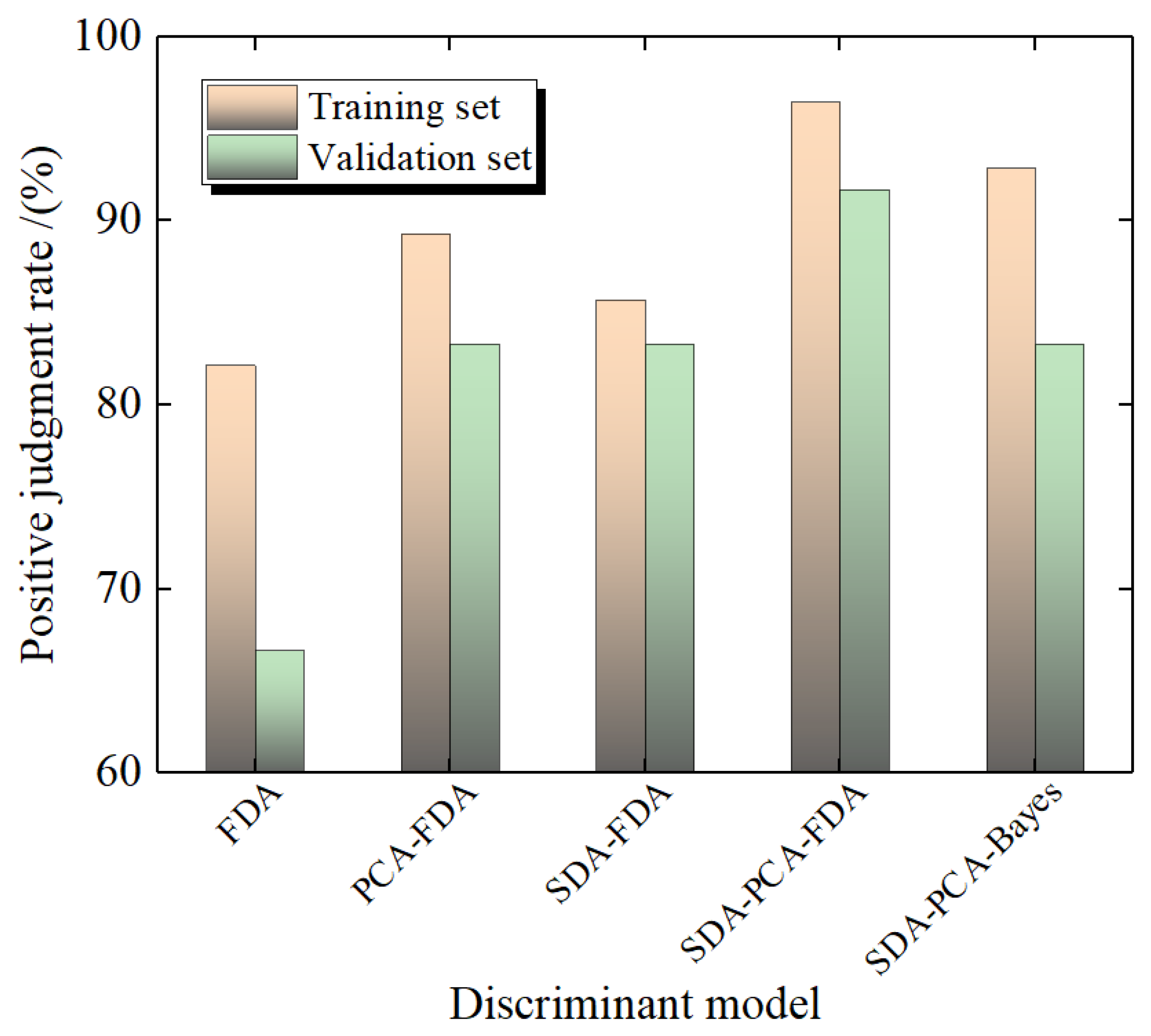
Following the methodology described in Section 2.3 of this paper, a traditional FDA model for non-mining-induced rupture of vertical shafts was established by directly employing all nine influencing variables as Fisher discriminant factors. This model was subsequently validated using both the re-substitution estimation method [30] on the training set and the testing sample set. The results, presented in Table 1 and Table 2, show correct classification rates of 82.14% for the training set and 66.67% for the validation set, indicating less-than-ideal discriminant performance (see Figure 2).
Considering that the non-mining-induced rupture of vertical shafts results from the combined effect of multiple factors, and the information carried by various influencing factors may partially overlap (e.g., the correlation between water level drawdown and relief groove compression amount), mutual interference can occur during mathematical analysis. To determine whether linear correlations exist among the variables, a multicollinearity diagnosis was performed on the collected data. The VIF (Variance inflation factor) value is the reciprocal of tolerance; generally, a value greater than 2 suggests potential collinearity. The output results, as shown in Table 3 [31], indicate a minimum VIF of 2.451, a maximum of 4.569, and an average of 3.532. Furthermore, based on the eigenvalues and condition indices (The indicator that measures the severity of multicollinearity between independent variables. The higher the conditional index, the more severe the multicollinearity problem in the data), it was found that the eigenvalues for dimensions 6–9 are approximately equal to zero, and all corresponding condition indices exceed 10 (multiple dimensions having eigenvalues near zero and condition indices greater 10 indicate collinearity among the influencing variables). The diagnostic results demonstrate severe multicollinearity among the multiple factors causing shaft rupture, suggesting they are not suitable for direct statistical analysis.
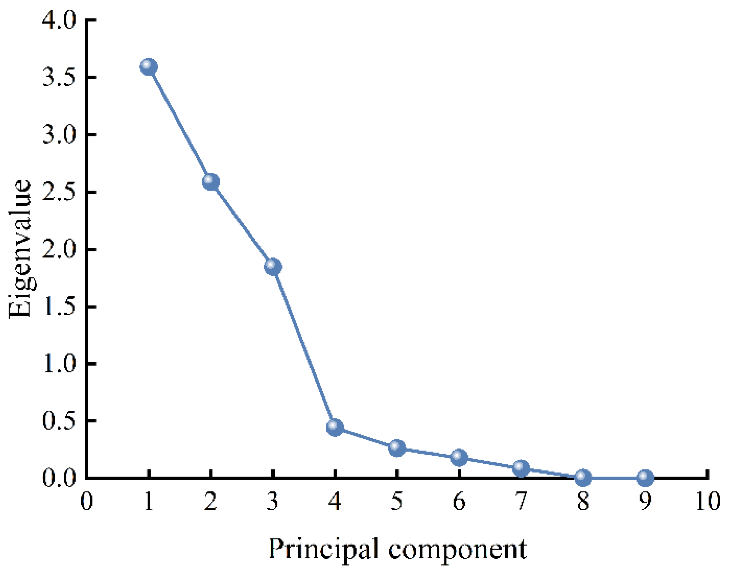
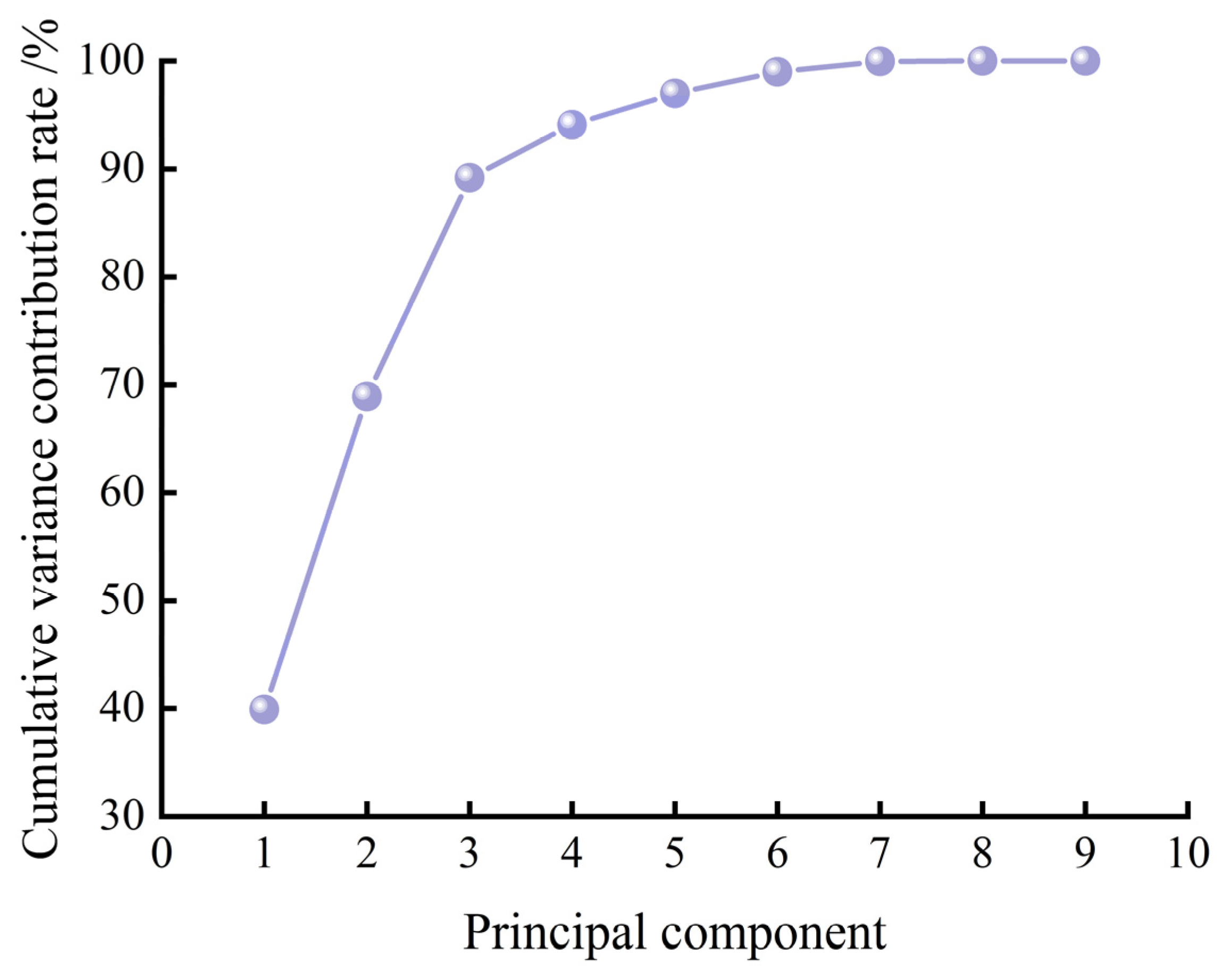
Due to information redundancy and the large number of variables studied, the accuracy of the discriminant model was not improved; instead, it led to low classification precision and a high misjudgment rate in the traditional Fisher discriminant model. As outlined in Section 2.1, the PCA method can reorganize the various influencing factors of shaft rupture into a smaller number of mutually independent principal components, thereby reducing the dimensionality of the modeling variables and minimizing the rate of ineffective information overlap. With the aid of SPSS25.0 statistical software, the sample data were processed using PCA. The output, shown in Table 4, includes the eigenvalues, variance contribution rates, and cumulative variance contribution rates of the principal components, along with the scree plot (shown in Figure 3). Following the principle of principal component extraction, the first three principal components were extracted, whose cumulative variance contribution rate reaches 89.189% (as shown in Figure 4). This indicates that these three principal components contain the vast majority of the information from the nine original influencing variables.
Since the object of analysis has been transformed, the information from the original variables needs to be standardized and assigned to the selected first three principal components to serve as discriminant indicators for the subsequent analysis. The Kaiser-normalized varimax rotation method was applied to obtain the principal component coefficient matrix (see Table 5), based on which the standardized expressions for the first three principal components were established (Formula (4)). In this formula, each variable Zγi is not the original variable but the standardized variable.
Y 1 = 0.148 Z γ 1 + 0.096 Z γ 2 + 0.327 Z γ 3 0.096 Z γ 4 + 0.397 Z γ 5 + 0.388 Z γ 6 + 0.007 Z γ 7 0.053 Z γ 8 0.142 Z γ 9 Y 2 = 0.239 Z γ 1 + 0.311 Z γ 2 0.014 Z γ 3 + 0.026 Z γ 4 0.059 Z γ 5 0.129 Z γ 6 + 0.249 Z γ 7 + 0.367 Z γ 8 + 0.429 Z γ 9 Y 3 = 0.375 Z γ 1 + 0.022 Z γ 2 + 0.021 Z γ 3 + 0.537 Z γ 4 + 0.046 Z γ 5 0.126 Z γ 6 0.042 Z γ 7 + 0.430 Z γ 8 0.032 Z γ 9
Similarly, following the method described in Section 2.3, the extracted first three principal components were utilized as discriminant factors to establish the PCA-FDA discriminant function:
y = 0.998 Y 1 + 0.121 Y 2 0.469 Y 3
From the above formula, the centroid of the discriminant function y for the ruptured shaft group was calculated to be −0.861, and for the non-ruptured group, 2.351. By calculating the function value for each sample and comparing its distance to these centroids, the discriminant results of the PCA-FDA model for all samples were obtained, as shown in Table 1 and Table 2. After PCA dimensionality reduction, the PCA-FDA model achieved a correct classification rate of 89.29% on the training set using re-substitution and 83.33% on the testing set. Compared to the traditional Fisher discriminant analysis, the model effectiveness in discriminating shaft rupture increased by 7.15% and 16.66%, respectively. However, for the Yanzhou Mining Area, which has experienced multiple incidents of non-mining-induced shaft rupture, the discriminant performance of the PCA-FDA model still falls short of practical requirements.
Considering the severe information redundancy among the original variables and their varying contributions to shaft rupture, the SDA method was employed to screen for significant variables with strong discriminant ability, thereby ignoring less influential variables to reduce the dimensionality of the data for establishing the Fisher discriminant model and effectively mitigating information redundancy. As described above, using the SDA method with the aid of SPSS25.0 statistical software, the original variables underwent a six-step screening process. This resulted in the selection of five significant indicators: γ7, γ6, γ8, γ5, and γ1, while the remaining variables were either not introduced or were eliminated after introduction. An SDA-FDA model was established using these five screened variables as discriminant factors to classify shaft rupture. The results, presented in Table 1 and Table 2, show that the SDA-FDA model achieved correct classification rates of 85.71% on the training set (via re-substitution) and 83.33% on the testing set. This represents an improvement of 3.57% and 16.66%, respectively, compared to the traditional Fisher discriminant model. When compared to the PCA-FDA model, the SDA-FDA model showed a lower correct classification rate on the training set but an identical rate on the testing set. Further comparison revealed that although the correct classification rates on the testing set were the same for both models, the specific misclassified shaft samples differed. The former model misclassified sample 03 but correctly classified sample 01, whereas the latter misclassified sample 01 but correctly classified sample 03. This indicates that both the PCA and SDA methods have their respective advantages in constructing the Fisher discriminant model for non-mining-induced shaft rupture. Combining these two methods could potentially lead to further improvements in the model discriminant performance.
As evidenced by the preceding analysis, although both the PCA-FDA and SDA-FDA discriminant models demonstrate superior discriminant ability and predictive performance compared to the traditional Fisher discriminant analysis model, and both provide valuable guidance for the prevention and control of non-mining-induced shaft rupture, their underlying emphases differ. The establishment of the SDA-FDA model focuses primarily on screening. The discriminant factors introduced into this model are optimally selected from various influencing factors, which neither alters the nature of each factor nor generates new variables. In contrast, the discriminant factors for the PCA-FDA model are derived through the synthesis of various influencing factors, introducing new components; thus, this model leans more towards reorganization. To leverage the respective strengths of both the SDA and PCA methods in the application of shaft rupture prevention and control, and to enhance the final model’s accuracy, the SDA and PCA methods are integrated based on the practical requirements of shaft rupture discrimination identified earlier. This integration leads to the establishment of a Fisher discriminant analysis model for non-mining-induced rupture of coal mine vertical shafts based on the SDA-PCA method.
Following this approach, as outlined in the research roadmap (Figure 1), the five significant indicators screened by the SDA method were used as the original variables for subsequent PCA. After performing the same analytical steps as employed in the PCA-FDA method, the eigenvalues of the resulting three new principal components were all greater than 1, and their cumulative variance contribution rate reached 92.632% (see Formula (6), Total variance explained). This indicates that these first three principal components contain the vast majority of the information from γ7, γ6, γ8, γ5, and γ1. Based on the component coefficients, the standardized expressions for PC1, PC2, and PC3 were calculated (Formula (6)).
P C 1 = 0.238 Z γ 1 + 0.852 Z γ 2 + 0.776 Z γ 6 + 0.451 Z γ 7 + 0.576 Z γ 8 P C 2 = 0.891 Z γ 1 + 0.156 Z γ 5 0.108 Z γ 6 0.444 Z γ 7 0.108 Z γ 8 P C 3 = 0.330 Z γ 1 + 0.240 Z γ 5 0.502 Z γ 6 0.595 Z γ 7 0.430 Z γ 8
Using the new principal components PC1, PC2, and PC3 as discriminant factors, and again following the methodology in Section 2.3 of the paper, the SDA-PCA-FDA discriminant function was established by leveraging the newly saved principal component data from SPSS25.0:
y = 1.568 P C 1 + 0.581 P C 2 + 0.757 P C 3
The centroid values of the discriminant function y for the ruptured and non-ruptured groups were calculated to be −1.573 and 1.481, respectively. The rupture status of each sample was then determined by calculating its function value and comparing its distance to these respective centroids. The validity of the discriminant function was tested. A smaller Wilks’ Lambda value and a larger chi-square test statistic indicate a greater ratio of between-group to within-group variance. A significance level of less than 0.05 further confirms that the discriminant effect of the function is statistically significant. Detailed results are presented in Table 6.

3.3. Validation of Discriminant Effectiveness

The effectiveness of the SDA-PCA-FDA discriminant model for non-mining-induced rupture of coal mine vertical shafts was validated. The re-substitution estimation method was used to reclassify the training sample set and validate the testing sample set, respectively. All 28 training samples were individually reclassified via re-substitution, and the model was tested using the 12 validation samples. The correct discriminant rates were 96.43% and 91.67%, respectively. Compared to the traditional FDA model, the PCA-FDA model, and the SDA-FDA model, the correct discriminant rate on the training set increased by 14.29%, 7.14%, and 10.72%, respectively. The correct discriminant rate on the testing set increased by 25.00%, 8.34%, and 8.34%, respectively. These results demonstrate that the Fisher discriminant analysis model based on the SDA-PCA method achieves a higher correct classification rate and exhibits superior performance, making it better suited for engineering applications. It can provide a valuable reference for predicting non-mining-induced rupture of vertical shafts in the Yanzhou Mining Area and under similar geological conditions. It is worth noting that SDA selected five key variables (γ7, γ6, γ8, γ5, γ1) from nine original variables, indicating that these five variables are the most important parameters for discriminating rupture. At the same time, the order in which they are introduced into the model also approximately reflects the strength of their discriminative ability.
To further validate the discriminant performance of the SDA-PCA-FDA model, its results were compared with those of a Bayesian model based on the same SDA-PCA method. (Preliminary calculations indicated that Bayesian models employing only SDA or PCA individually yielded lower correct classification rates on both the training and testing sets compared to the SDA-PCA-Bayes discriminant analysis model; therefore, these are not discussed further in this paper). As two important methods in multivariate statistical discriminant analysis, the key difference between Fisher discriminant analysis and Bayesian discriminant analysis lies in the fact that the former does not assume a specific sample distribution, focusing solely on maximizing the ratio of between-group to within-group variance. The latter, however, starts from the multivariate distribution of the samples, fully utilizing the information provided by the probability density of the multivariate normal distribution to classify test samples. Comparing these two methods effectively assesses the model predictive performance.
The fundamental principle of Bayesian discrimination is to describe prior knowledge using a prior distribution, then, based on this understanding of the prior, summarize the information and make new inferences, i.e., perform prediction via the posterior distribution [29]. Using SPSS25.0 statistical software and the training sample set from Table 1, a Bayesian model based on the SDA-PCA method was established. The three principal components (PC1, PC2, and PC3), derived from the SDA screening and PCA synthesis described earlier, served as the discriminant factors. The discriminant functions for the rupture and non-rupture groups are given by Formulas (5) and (6), respectively. The variables of each sample are substituted into these two Bayesian discriminant functions. The sample is then assigned to the category corresponding to the larger function value.
B 1 = 2.017 P C 1 + 1.259 P C 2 0.574 P C 3 1.595
B 2 = 3.474 P C 1 0.160 P C 2 + 3.396 P C 3 2.669
The 28 training samples and the 12 testing samples were, respectively, substituted into the aforementioned discriminant functions for classification. The results, presented in Table 1 and Table 2, show a correct classification rate of 92.86% for the training set (via re-substitution) and 83.33% for the testing set. Both rates are lower than those achieved by the Fisher discriminant analysis model established based on the SDA-PCA method. The discriminant accuracy rates of the different models are summarized in Table 7. As evident from the table, the SDA-PCA-FDA model demonstrates superior performance in discriminating and predicting non-mining-induced rupture of vertical shafts in the Yanzhou Mining Area. It can be effectively applied in practical engineering to assess shaft rupture conditions, thereby providing crucial support for the prevention and control of shaft rupture and for ensuring the safe operation of shafts. It is worth noting that the SDA-PCA-FDA model is mainly applicable to areas with similar geological conditions as the Yanzhou mining area, and its core feature is the presence of deep and loose alluvial layers. At the same time, this model also has certain limitations, mainly including the fact that the establishment of the model depends on the dataset of a specific region, which needs to be validated when applied to new regions; Moreover, this model belongs to static discrimination and cannot dynamically predict the evolution of rupture time, degree, etc.

4. Engineering Prediction

The main shaft, auxiliary shaft, and east air shaft of a coal mine in the Yanzhou Mining Area have net diameters of 8.0 m, 7.5 m, and 5.5 m, respectively. All shafts penetrate unconsolidated Quaternary alluvial strata with a thickness exceeding 150 m. Specifically, the overburden thickness is 189.31 m for the main shaft, 190.41 m for the auxiliary shaft, and 176.45 m for the east air shaft. Due to mining activities, the aquifer at the base of the alluvial layer has experienced a continuous decline in water level. This has led to multiple incidents in recent years, including longitudinal bending deformation of the shaft guides and spalling of concrete within the rupture zone near the interface between the alluvium and bedrock, seriously threatening mine safety. Preventive engineering measures were implemented last year to ensure normal shaft operation. However, with the ongoing expansion of mining operations and a further drop in the aquifer level, the risk of rupture persists for all shafts. Therefore, a renewed assessment of the rupture status for these three shafts was required this year. The SDA-PCA-FDA discriminant model for non-mining-induced rupture of coal mine vertical shafts, established in this study, was applied. The safety state of the shafts was evaluated by predicting unknown data based on the regression function derived from the existing data [32], or directly based on new measured data. The evaluation results, presented in Table 8, are as follows: The y-values for the auxiliary shaft and the east air shaft are 2.064 and 2.301, respectively. Both values are closer to the centroid of the non-ruptured group (1.481), indicating a safe state. In contrast, the y-value for the main shaft is −0.658, which is closer to the centroid of the ruptured group (−1.573), suggesting a risk of renewed rupture and necessitating preventive engineering measures. This discriminant outcome is consistent with the actual situation.

5. Sustainable Governance Application

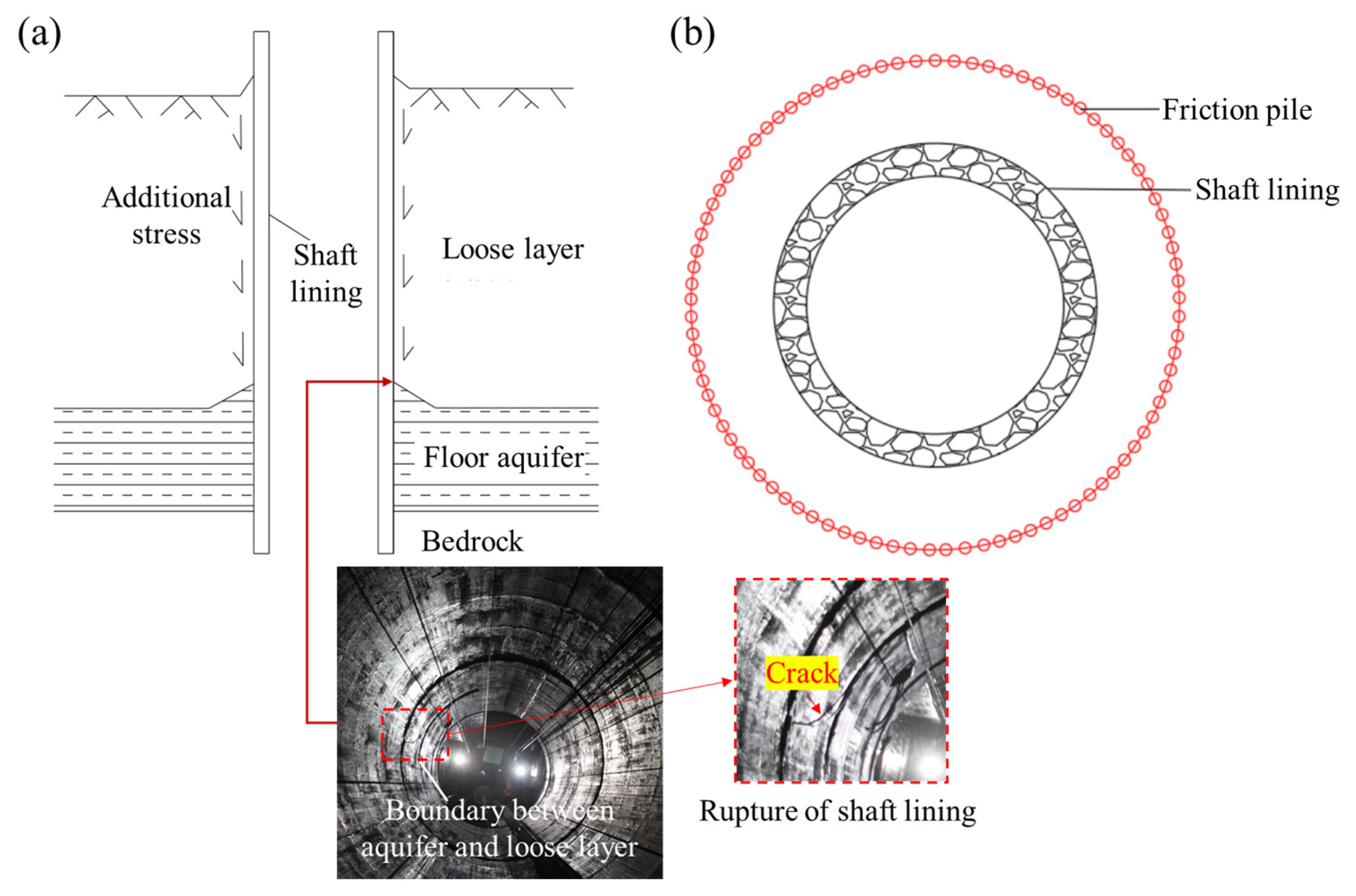
As illustrated in Figure 5a, the consolidation and compression of the overlying unconsolidated soil layer generate additional stress on the inner shaft wall. Rupture occurs when this stress exceeds the strength of the shaft lining. Based on this mechanism, the rupture of the main shaft, as predicted by the SDA-PCA-FDA model, requires treatment. The primary focus lies on how to reduce the additional stress on the shaft lining by mitigating stratum settlement, thereby achieving protection. Current traditional domestic methods for addressing shaft deformation and failure primarily include the shaft ring reinforcement method, the relief groove method, the grouting method, and the sleeve wall reinforcement method. Due to limitations in their sustainability duration, treatment cycle, economic efficiency, and the necessity for production stoppage, these four methods fail to fundamentally resolve the issue of increasing additional stress caused by settlement and consolidation; thus, they merely address the symptoms rather than the root cause. This paper proposes the “Friction Pile Method” for the preventive treatment of rupture in operational shafts. This method involves construction external to the shaft (see Figure 5b), causing no disruption to coal production and providing sustainable, long-term protection. The core concept of the friction pile method is to construct a “protective sleeve” composed of solidified friction piles around the shaft. This sleeve works by utilizing the frictional resistance with the surrounding soil layer to inhibit its consolidation settlement, thereby reducing the vertical additional stress acting on the shaft wall. The specific construction procedure can be broken down into the following steps: (1) Determine the key parameters based on NM2dc numerical simulation, including pile height, pile diameter and spacing, and pile-to-shaft distance. (2) Arrange the pile positions symmetrically around the shaft, typically on a circle with a radius of 10 m centered on the shaft axis. (3) Use large drilling rigs to bore holes at the predetermined pile locations. The borehole diameter must meet the final designed pile diameter requirements, and the depth should align with the simulation results mentioned above. (4) Lower pre-fabricated high-strength steel pipes into the drilled holes. These pipes serve as the skeleton and grouting channels for the friction piles, and their connections must be robust to ensure structural integrity. (5) Inject a specific cement-based grout into the holes under high pressure through grouting pipes pre-installed at the bottom of the steel pipes. (6) Under pressure, the grout permeates the soil around the steel pipes and ultimately fills the interior of the pipes and the annulus between the pipes and the borehole wall, forming a cylindrical composite pile structure. As a result, by reinforcing the shaft surrounding rock through the formation of a friction pile structure, it effectively inhibits the consolidation settlement of the unconsolidated layer, fundamentally resolving the chain reaction of “aquifer water level decline—stratum compression—additional stress generation—shaft rupture”.

5.1. Determination of Friction Pile Parameters via Numerical Simulation

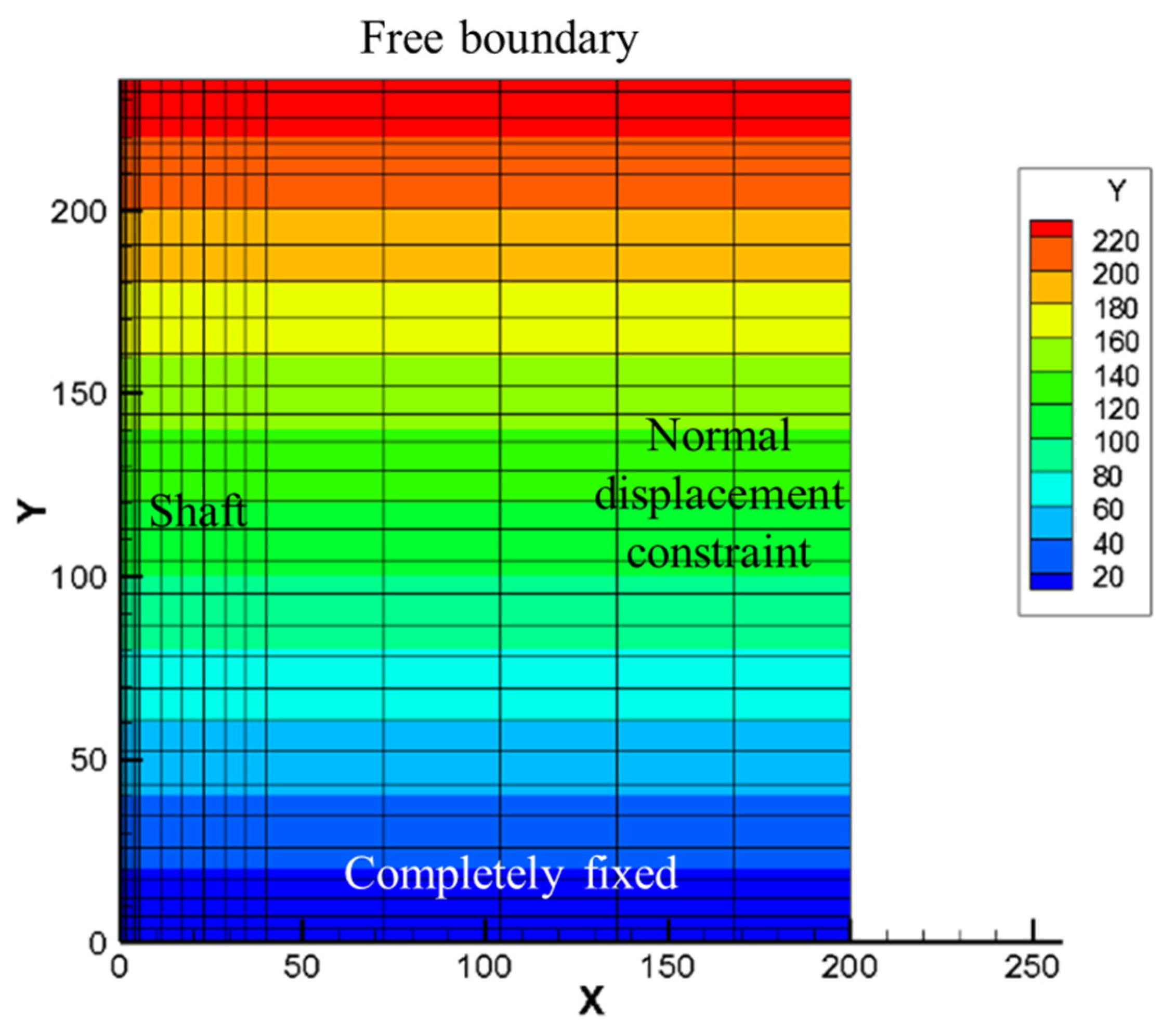
The simulation was conducted using the specifically developed NM2dc numerical modeling software. This software is based on the finite element method and suitable for common geotechnical problems such as plane strain issues and consolidation deformation, and offers unique advantages for studying non-mining-induced shaft rupture caused by stratum settlement. The key structural parameters determined for the friction piles include their height, stiffness coefficient, and the spacing between the friction piles and the shaft wall. Based on a shaft with an inner diameter of 8 m and an outer diameter of 11 m, the potential dewatering point was identified at a depth of −223 m (i.e., the shaft failure location) through previous long-term monitoring. The designed simulation model used the auxiliary shaft as the central axis, extending radially outward 200 m in width, and ranging vertically from the ground surface to the bedrock weathering zone, resulting in a total depth of 235.73 m (see Figure 6). The numerical simulation in this study was conducted using the NM2dc finite element analysis platform, establishing a two-dimensional model that accounts for soil-structure interaction. The model was discretized into 620 six-node triangular elements, connected through 672 nodes. In terms of element selection, higher-order elements suitable for large deformation analysis of geotechnical materials were specifically adopted, with mesh refinement implemented around the shaft and friction pile areas to ensure sufficient computational accuracy in these stress concentration zones. Regarding material constitutive models, all soil strata were simulated using the Mohr-Coulomb elastoplastic model, with detailed geotechnical parameters including elastic modulus, cohesion, internal friction angle, unit weight, and permeability coefficients for each layer provided in Table 9. The shaft lining was modeled using a linear elastic model based on C40 concrete characteristics, with an elastic modulus of 30 GPa and Poisson’s ratio of 0.2. The friction piles were similarly simplified as linear elastic materials, but their equivalent elastic modulus incorporated a stiffness reduction coefficient of 0.9 to account for the pile-soil interface interaction effects. The boundary conditions were set as follows: the model bottom (bedrock surface) was fully fixed, restricting displacements in all directions; the model sides were constrained with normal displacement constraints, allowing vertical free settlement; and the model top was set as a free boundary to realistically reflect surface settlement deformation. The loading scenario was implemented through nine consecutive loading steps, simulating the five-year formation consolidation settlement process caused by pore water pressure changes resulting from continuous aquifer dewatering.
In Table 9, K is the elastic modulus, Kur is the unloading-reloading modulus; Rf is the failure ratio; C and φ are the cohesion and internal friction angle, respectively; Δφ is the logarithmic reduction value of the internal friction angle with confining pressure; K0, Kns, and Kvs are the lateral pressure coefficient, horizontal permeability coefficient, and vertical permeability coefficient, respectively. The above parameters are determined based on on-site engineering geological and hydrogeological surveys, systematic indoor geotechnical tests, regional engineering specifications, and parameter inversion combined with on-site monitoring data.

5.1.1. Friction Pile Stiffness and Height

As shown in Table 10, five simulation schemes were established. These are divided into two categories: vertical schemes and horizontal schemes. The vertical schemes involve varying the friction pile height, while the horizontal schemes involve varying the stiffness coefficient. Specifically, Schemes 1, 2, and 3 all employ a friction pile height of 112.86 m, with stiffness coefficients set to 0.5, 0.1, and 0.9, respectively. In contrast, Schemes 4 and 5 both use a stiffness coefficient of 0.5, only varying the friction pile height for simulation. Among them, Scheme 4 selects a friction pile height of 49.86 m, and Scheme 5 selects a height extending from the ground surface to the bedrock weathering zone, i.e., 235.73 m. This scheme design determines the optimal friction pile height and stiffness coefficient by varying parameters along different dimensions.
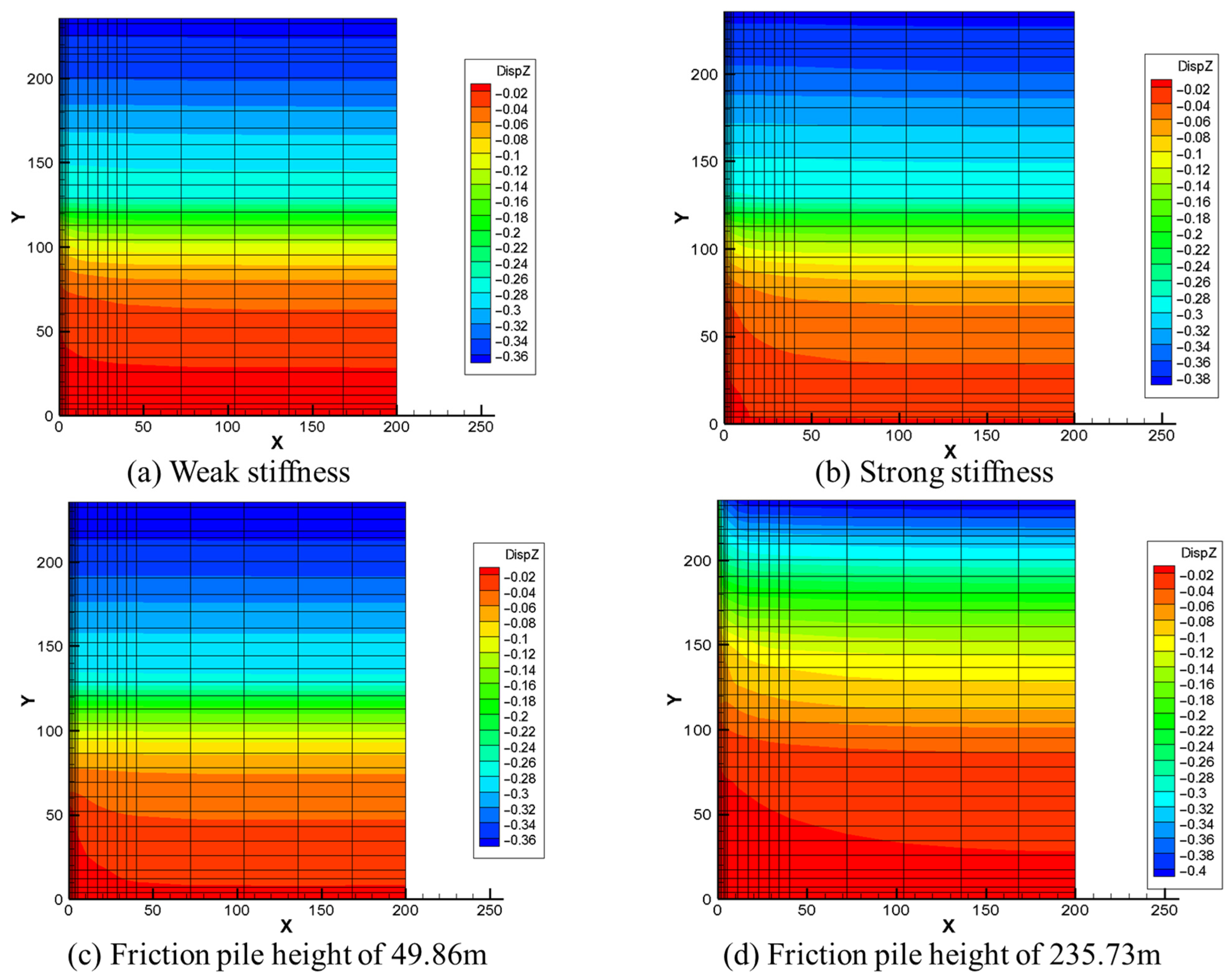
Horizontal Schemes, comprising Schemes 1, 2, and 3, were designed by varying only the friction pile stiffness. Vertical Schemes, comparing Schemes 1, 4, and 5, were used to determine the optimal friction pile height. The NM2dc simulation results are presented below. Figure 7a shows the contour map of stratum compression under low stiffness. It can be observed that, within the friction pile zone, the stratum settlement in the X-direction changes unevenly with increasing radial distance from the friction pile axis. Within the 0–40 m range, the settlement values are relatively small, ranging from 0.07 m to 0.161 m, but the settlement variation is significant. Within the 40–200 m range, the settlement values are larger, ranging from 0.161 m to 0.162 m, but the settlement variation is minimal. Beyond the friction pile zone, across the 0–200 m range in the X-direction, the stratum settlement is relatively large, essentially uniform at about 0.371 m. Figure 7b shows the contour map of stratum compression under high stiffness. Within the friction pile zone, the stratum settlement in the X-direction also changes unevenly with increasing radial distance. Within the 0–70 m range, the settlement values are relatively small, ranging from 0.07 m to 0.177 m, but the settlement variation is significant. Within the 70–200 m range, the settlement values are larger, ranging from 0.177 m to 0.178 m, but the settlement variation is minimal. Beyond the friction pile zone, across the 0–200 m range in the X-direction, the stratum settlement is relatively large, essentially uniform at about 0.377 m. The comparison reveals that friction piles with higher stiffness exert a greater influence on the stratum.
Under the condition of a stiffness coefficient of 0.5, Figure 7c presents the simulation results for a friction pile height of 49.86 m, while Figure 7d shows the results for a height of 235.73 m. As observed from Figure 7c, within the friction pile zone, the stratum settlement in the X-direction varies unevenly with increasing radial distance from the pile axis. In the range of 0–40 m, the settlement values are relatively small, ranging from 0.004 m to 0.04 m, but the magnitude of settlement change is significant. In the 40–200 m range, the settlement values are larger, between 0.04 m and 0.041 m, yet the settlement variation is minimal. Outside the friction pile zone, across the 0–200 m range in the X-direction, the stratum settlement is relatively high and essentially uniform at approximately 0.381 m. Figure 7d indicates that, within the friction pile zone, the X-direction stratum settlement also changes unevenly with increasing radial distance. In the 0–70 m range, settlement values are relatively small, ranging from 0.037 m to 0.418 m, but with considerable variation. In the 70–200 m range, settlements are larger, between 0.418 m and 0.419 m, with minimal variation. Based on this analysis, although the 235.73 m high friction pile exerts a greater influence on stratum settlement, it also results in higher absolute settlement values. Therefore, it is concluded that appropriately increasing the friction pile height can effectively enhance the treatment efficacy of the friction pile method.
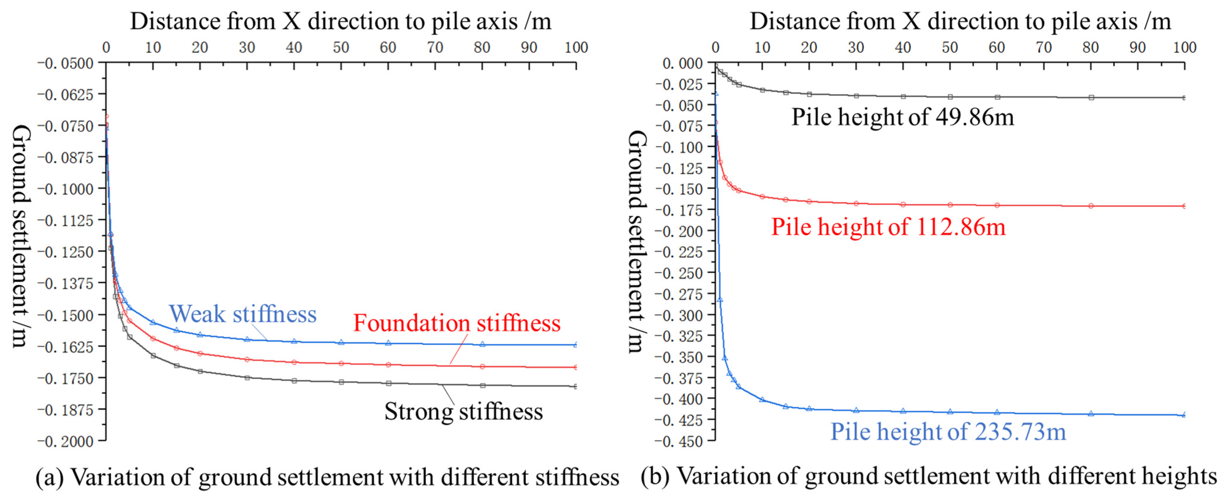
The survey line method was employed to compare the different schemes. Based on the simulation results, survey lines were established at the failure location for Schemes 1, 2, and 3, and at the interface between the friction piles and the stratum for Schemes 1, 4, and 5. The stratum settlement along these survey lines for each scheme was plotted as curves for comparison, with the results shown in Figure 8a,b.
Figure 8a shows the stratum settlement variation curves at the failure location for schemes with different stiffness coefficients. The results indicate that within the X-direction range of 0–50 m, the settlement at the failure location changed under all three schemes. Among them, the high-stiffness scheme exhibited the most pronounced change in stratum settlement, indicating the best governance effect. In contrast, the low-stiffness scheme showed the smallest variation in settlement, suggesting a poorer governance effect. Within the X-direction range of 50–100 m, the stratum settlements of all three schemes stabilized. The high-stiffness scheme resulted in the largest settlement, while the low-stiffness scheme yielded the smallest settlement. However, due to the minor differences in settlement values, their impact was not considered significant. As shown in Figure 8b, within the X-direction range of 0–50 m, the settlement values changed under all three schemes. Among them, the scheme with a friction pile height of 235.73 m exhibited the largest settlement variation, while the scheme with a height of 49.86 m showed the smallest settlement variation. Within the X-direction range of 50–100 m, the stratum settlements of all three schemes remained essentially constant, stabilizing at a plateau. However, the differences in settlement values among the schemes were significant. Since the survey lines were set at the contact interface, and the contact interface positions varied with different friction pile heights, this could not serve as a definitive criterion for evaluation. Therefore, this study selected a moderate solution, adopting a friction pile height of 112.86 m.
Furthermore, the influence percentage of each scheme was calculated as the ratio of the settlement suppressed at the failure location to the stabilized settlement amount. The results, presented in Table 11, show that when comparing different stiffness coefficients, the high-stiffness condition yielded the highest reduction percentage of settlement at the failure location, at 31.3%. This indicates that friction piles with high stiffness have the greatest influence on stratum settlement. Therefore, a stiffness coefficient of 0.9 was selected. When comparing different friction pile heights—specifically, Schemes 1, 4, and 5—the results demonstrate that the scheme with a pile height of 112.86 m achieved the highest influence percentage, reducing the stratum settlement at the failure location by 30.9%. Consequently, a friction pile height of 112.86 m was adopted, which aligns with the determination made using the survey line method. In summary, for the selection of the friction pile’s height and stiffness, the optimal parameters are a height of 112.86 m and a stiffness coefficient of 0.9 for the treatment.

5.1.2. Friction Pile to Shaft Wall Spacing

Building upon the established friction pile stiffness and height, four additional schemes were designed by varying two parameters: the presence or absence of friction piles and the spacing between the piles and the shaft wall. These schemes were simulated to calculate stratum settlement and thereby determine the optimal arrangement of the friction piles. The specific scheme design is shown in Table 12. Schemes 1 to 3 were configured with friction pile to shaft wall spacings of 5 m, 10 m, and 15 m, respectively. Scheme 4 served as a comparative baseline where no friction piles were installed.
As shown in Figure 9a, within the vertical extent where friction piles are installed at a distance of 5 m from the shaft wall, the stratum settlement in the X-direction exhibits non-uniform variation with increasing radial distance from the shaft axis. Specifically, within the 0–15 m range, the stratum settlement initially stabilizes, with values ranging between 0.005 m and 0.015 m. Within the 15–200 m range, the stratum settlement gradually decreases due to the influence of the friction piles until this influence diminishes, and the settlement stabilizes again, with values ranging from 0.015 m to 0.171 m. Outside the vertical extent of the friction piles, within the 0–20 m range, the stratum settlement is relatively small due to the influence of the shaft wall, with values between 0.023 m and 0.240 m. Within the 20–200 m range, the stratum settlement gradually decreases under the influence of the shaft wall, with values ranging from 0.240 m to 0.392 m. In Figure 9b, within the vertical extent of the friction piles, the stratum settlement in the X-direction also shows non-uniform variation with increasing radial distance. Here, within the 0–15 m range, the settlement initially stabilizes, with values between 0.005 m and 0.013 m. Within the 15–200 m range, the settlement gradually decreases under the influence of the friction piles until this effect fades, and the settlement stabilizes, with values ranging from 0.013 m to 0.151 m. Outside the friction pile zone, within the 0–20 m range, the settlement remains relatively small due to the shaft wall’s influence, with values between 0.019 m and 0.210 m. In the 20–200 m range, the settlement gradually decreases influenced by the shaft wall, with values from 0.210 m to 0.361 m. When the friction pile to shaft wall spacing is 15 m (see Figure 9c), the stratum settlement in the X-direction varies non-uniformly with increasing radial distance. In the 0–15 m range, the settlement first stabilizes, with values between 0.005 m and 0.017 m. Within the 15–200 m range, the settlement gradually decreases due to the friction piles’ influence until it vanishes, and the settlement stabilizes, with values ranging from 0.017 m to 0.191 m. Beyond the vertical extent of the friction piles, within the 0–20 m range, the settlement is relatively small under the shaft wall’s influence, with values between 0.026 m and 0.310 m. In the 20–200 m range, the settlement gradually decreases influenced by the shaft wall, with values from 0.310 m to 0.423 m.
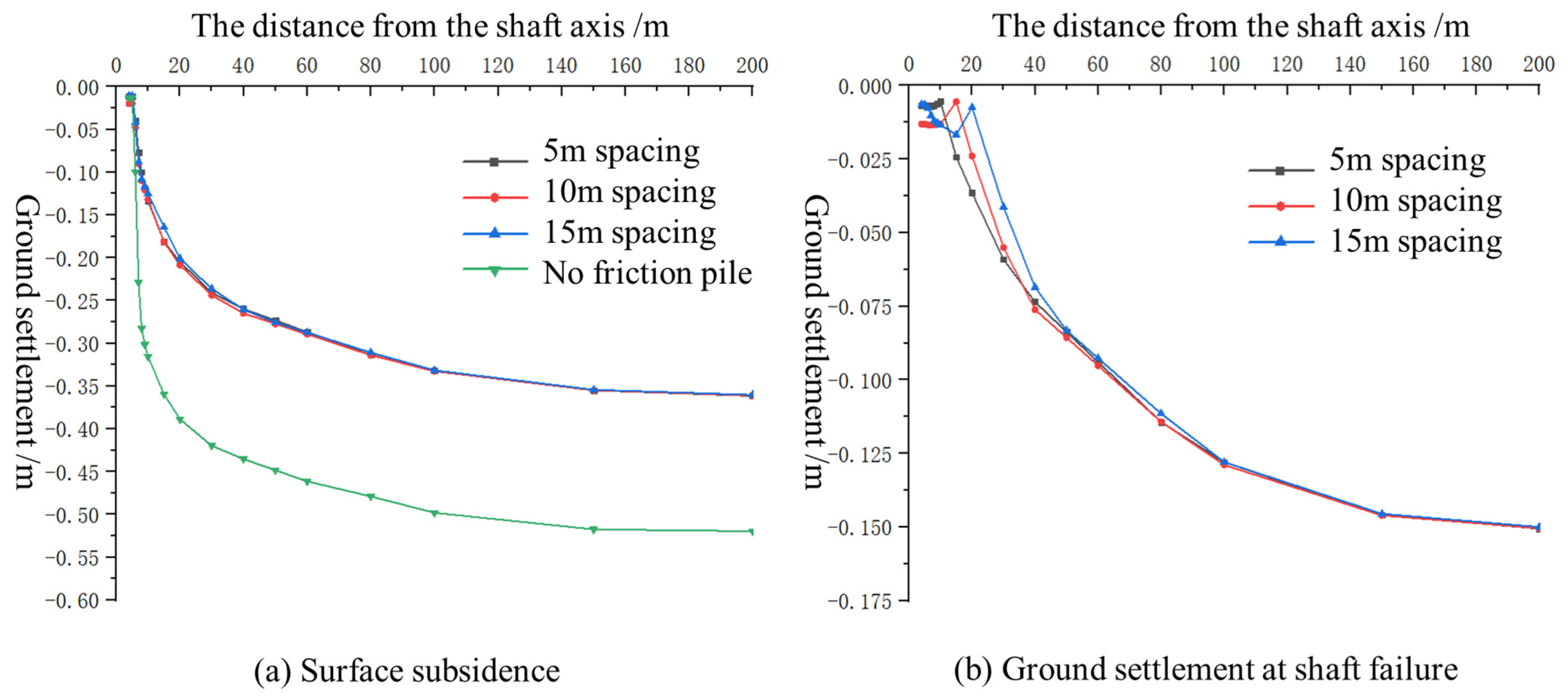
To determine the relationship between the friction pile-to-shaft wall spacing and the governance effectiveness, the optimal scheme was selected through comparative analysis of stratum settlement. Figure 10 shows the stratum settlement variation curves under different friction pile spacings, where Figure 10a depicts the settlement at the ground surface, and Figure 10b illustrates the settlement variation curve at the failure location. As shown in the figure, the settlement curves at the ground surface for Schemes 1 to 3 are essentially identical. In contrast, Scheme 4, which involved no friction piles, exhibited significantly greater stratum settlement compared to the other three schemes. This demonstrates that the installation of friction piles can effectively reduce stratum settlement at the ground surface; however, varying the distance between a single friction pile and the shaft wall has negligible impact on the settlement at this location. From Figure 10b, it can be observed that within the X-direction range of 0–40 m, the stratum settlement for all three schemes initially increases, then abruptly decreases, before increasing again until it stabilizes. Among them, the curve of Scheme 3 declines more slowly, while that of Scheme 1 declines most rapidly. This indicates that appropriately increasing the spacing between friction piles and the shaft wall can effectively enhance the influence of the friction piles on stratum settlement.
The aforementioned analysis supports the conclusion that appropriately increasing the spacing between the friction piles and the shaft wall can effectively enhance their influence on stratum settlement. However, as the final stabilized settlement values differ among the schemes, it does not follow that a larger spacing invariably yields better governance effectiveness. Therefore, a determination based on the calculated influence degree is necessary. As shown in Table 13, the influence degree on the settlement at a radial distance of 1 m from the shaft wall at the failure location was calculated for each scheme. Post-processing of the data revealed settlement reduction percentages of 95.3% for Scheme 1, 96.0% for Scheme 2, and 94.0% for Scheme 3. Thus, it can be concluded that Scheme 2, corresponding to a pile-to-shaft wall spacing of 10 m, provides the optimal governance effectiveness.
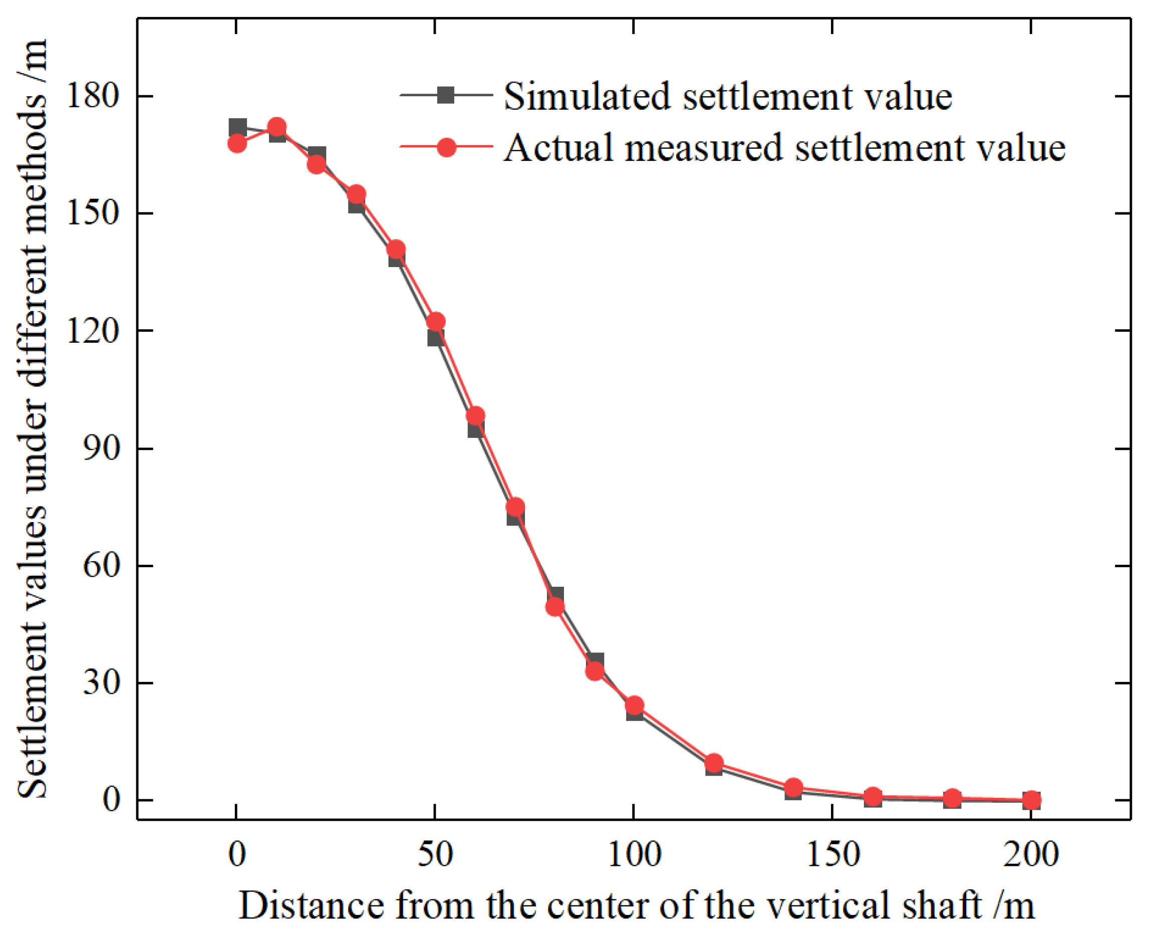
To ensure the reliability of the numerical model, this study validated it against field monitoring data. Using historical data from surface settlement monitoring points around the auxiliary shaft in the mining area, the actual water level drawdown was input as the load into the model. The simulated surface settlement values were then compared with the measured values. The results show that the development trend of the surface settlement calculated by the model agrees well with the measured data, with an average relative error of less than 8% at key points by the end of the simulation period. This error margin is within acceptable engineering limits, demonstrating that the established numerical model can effectively reflect the consolidation settlement behavior of the stratum under aquifer dewatering and is suitable for subsequent parameter analysis of friction piles.
On the other hand, the validation specifically focused on the surface settlement profile along a predetermined monitoring section crossing the shaft centerline. This section contained 16 fixed monitoring points at predetermined locations (0, 10, 20, 30, 40, 50, 60, 70, 80, 90, 100, 120, 140, 160, 180, and 200 m from the shaft center). Both simulated and field measurements were taken at these identical positions to ensure direct comparability. The verification results demonstrate close alignment between simulated and measured values: the maximum simulated settlement was 172.4 mm at the shaft center (0 m), while the maximum measured settlement was 172.5 mm at 10 m from the center (see Figure 11), representing a negligible relative error of 0.06%. Regarding the settlement influence range, the simulation showed settlement attenuation below 1 mm at 160 m from the center, consistent with field measurements which recorded <1 mm settlement at 180 m. Quantitative analysis revealed average relative errors of 3.5% within the primary influence zone (0–100 m) and 5.8% in the secondary influence zone (100–200 m). This spatial validation confirms that the numerical model accurately captures not only temporal settlement patterns but also the complete spatial distribution of the displacement field, thereby verifying the reliability of the simulation results for subsequent parameter analysis.

5.2. Comparative Analysis of Governance Scheme Sustainability

To prevent repeated shaft rupture, a comprehensive analysis integrating technical feasibility with economic sustainability indicators should serve as the basis for comparing and selecting different governance schemes. Five distinct schemes were designed:
(1)
Scheme 1: Chemical grouting after wall penetration within the 213 m to 230 m depth range, combined with creating a relief groove at 223 m depth.
(2)
Scheme 2: Cement grouting after wall penetration within the 213 m to 230 m depth range, combined with creating a relief groove at 223 m depth.
(3)
Scheme 3: Shaft ring reinforcement within the 213 m to 230 m depth range, combined with creating a relief groove at 223 m depth.
(4)
Scheme 4: Ground grouting to reinforce the unconsolidated strata, combined with shaft ring reinforcement.
(5)
Scheme 5: Implementation of the friction pile method at a horizontal distance of 10 m from the shaft wall.
Schemes 1 and 2 both combine wall-penetration grouting with the relief groove method, differing primarily in the grouting material used. Scheme 1 employs chemical grouting materials, whereas Scheme 2 utilizes cement grouting. Since the failure location of the auxiliary shaft is at a depth of 223 m, the grouting section is set from 213 m to 230 m, spanning 17 m, and the relief groove is precisely located at the failure depth of 223 m. Scheme 3 involves the combined application of shaft ring reinforcement and the relief groove method [33]. The section for shaft ring reinforcement corresponds to the grouting section in the wall-penetration grouting schemes, involving the addition of a circumferential concrete inner lining to the shaft wall, alongside creating a relief groove at 223 m depth. Scheme 4 integrates the ground grouting method with shaft ring reinforcement. As ground grouting addresses the root cause of the shaft failure and shaft ring reinforcement provides safety protection, this scheme does not simultaneously incorporate a relief groove. Scheme 5 employs the innovative friction pile method for shaft governance. This involves deploying four drilling rigs on the surface. At a depth of 119 m, branching is performed, and multiple individual pipe piles are installed at a horizontal distance of 10 m from the shaft wall. Grouting is then conducted inside the steel pipes to solidify them, ultimately forming a pile group structure around the shaft to achieve the goal of protecting the shaft wall.

5.2.1. Economic Budget Analysis

The five schemes differ in their governance effectiveness, costs, and construction durations. Therefore, the economic efficiency of each scheme was calculated and analyzed. The results are summarized in Table 14, Schemes 1, 2, and 3 have relatively lower budgeted costs, ranging from 1.0 to 1.5 million CNY, while Schemes 4 and 5 have higher budgets, at 6.97 million CNY and 5.17 million CNY, respectively. Based on the predicted construction durations in the table, the chemical and cement wall-penetration grouting methods require 55 days and 50 days, respectively. The shaft ring reinforcement method has the shortest duration, requiring approximately 20 days. In contrast, the ground grouting method and the friction pile method have longer durations, at 150 days and 140 days, respectively. Analysis of the construction processes reveals that both the shaft ring reinforcement method and the wall-penetration grouting methods involve work inside the shaft, thus requiring production stoppage during implementation and causing significant disruption to mining operations. Conversely, the ground grouting and friction pile method treat the strata externally around the shaft, resulting in minimal disruption to production.

5.2.2. Analysis of Scheme Advantages and Disadvantages

The advantages and disadvantages of the different schemes are summarized in Table 15. Considering that the mine shaft has already experienced failure at a depth of 223 m and requires treatment, and given the high production efficiency of the mine, the impact of internal shaft construction during the treatment period must be considered. As the wall-penetration grouting method causes significant production disruption, Schemes 1 and 2 are not recommended. Based on the stratum structure, the aquifer at the shaft failure location exhibits strong water richness and a high water head, posing substantial safety risks after failure. Although the shaft ring reinforcement method can rapidly control failure propagation, its effective duration is short, making it unsuitable as a long-term treatment solution. Therefore, Scheme 3 is not recommended. Comparing Scheme 4 (ground grouting) and Scheme 5 (friction pile method), ground grouting performs poorly in controlling additional stress and incurs construction costs 1.8 million CNY higher than the friction pile method. In contrast, the friction pile method addresses the root cause by mitigating additional stress. Its characteristic of requiring no internal shaft construction minimizes impact on production. Although the construction process is complex and demands high technical standards, it ensures safety during implementation, aligning with the specific characteristics of this mine shaft. Consequently, Scheme 5, the friction pile method, is recommended. The key treatment parameters for this method have already been determined through numerical simulation.

6. Conclusions

(1) Factors including the thickness of the alluvial layer, construction method, service year ratio, shaft net diameter, water level drawdown, relief groove compression rate, rupture degree, compression rate of the unconsolidated alluvial layer, and treatment method were selected for analysis. Integrating the advantages of both PCA and SDA data analysis methods, the five discriminant factors optimally selected by the SDA method were subsequently subjected to PCA. This process generated three new principal components, ultimately leading to the establishment of the FDA model for non-mining-induced rupture of vertical shafts in the Yanzhou Mining Area based on the SDA-PCA method, namely the SDA-PCA-FDA model.
(2) Compared to the traditional FDA model, the PCA-FDA model, and the SDA-FDA model, the SDA-PCA-FDA model achieved increases in the correct classification rate of 14.29%, 7.14%, and 10.72%, respectively, on the training set, and 25.00%, 8.34%, and 8.34%, respectively, on the testing set, demonstrating superior discriminant performance.
(3) Taking the main shaft, auxiliary shaft, and east air shaft of a mine in the Yanzhou Mining Area as examples, the SDA-PCA-FDA model was applied to predict their safety states. The results indicate that both the auxiliary shaft and the east air shaft are in a safe state, whereas the main shaft is at risk of rupture, necessitating preventive engineering measures. This prediction outcome is consistent with the actual situation.
(4) Addressing the main shaft rupture predicted by the model, the specially developed NM2dc numerical software was used to determine the key parameters for the friction pile treatment. These include a friction pile height of 112.86 m, a stiffness coefficient of 0.9, and an optimal pile–shaft wall spacing of 10 m for the most effective aquifer dewatering treatment. Based on technical feasibility and supplemented by sustainability application as an economic indicator, a comprehensive analysis of five different treatment schemes was conducted, verifying the sustainable governance advantages of the friction pile method.

Author Contributions

Conceptualization, Q.G. and G.Y.; methodology, Q.F. and S.L.; validation, G.Y.; formal analysis, Q.G.; resources, S.L.; writing—original draft preparation, Q.G.; writing—review and editing, G.Y. and Q.L.; supervision, Q.M.; project administration, validation C.L.; funding acquisition, Q.F. All authors have read and agreed to the published version of the manuscript.

Funding

This work is supported by State Key Laboratory for Tunnel Engineering (No. TESKL202418), the National Natural Science Foundation of China (Grant Nos. 52204164, 52404156).

Data Availability Statement

The original contributions presented in this study are included in the article. Further inquiries can be directed to the corresponding authors.

Conflicts of Interest

Authors declare that the research was conducted in the absence of any commercial or financial relationships that could be construed as a potential conflict of interest.

References

  1. Li, Z.; Yang, G.; Wang, B.; Wang, J. Study on Unfrostered Water Content and Strength Characteristics of Saturated Sandstone During Thawing Process. Sci. Rep. 2025, 15, 17641. [Google Scholar] [CrossRef]
  2. Rong, J.; Wang, B. Deformation and Instability Mechanisms of a Shaft and Roadway Under the Influence of Rock Mass Subsidence. Appl. Sci. 2025, 15, 163. [Google Scholar] [CrossRef]
  3. Yu, J.; He, H.; Liu, Z.; He, X.; Zhou, F.; Song, Z.; Yang, D. Analysis of Spatiotemporal Characteristics of Microseismic Monitoring Data in Deep Mining Based on ST-DBSCAN Clustering Algorithm. Processes 2025, 13, 2359. [Google Scholar] [CrossRef]
  4. Xu, Y.; Fu, W. Research on Coupling Adsorption Experiments for Wall–Climbing Robots in Coal Mine Shafts. Processes 2023, 11, 2016. [Google Scholar] [CrossRef]
  5. Chen, L.; Yang, X.; Guo, L.; Yu, S. Analysis of Rock Mass Energy Characteristics and Induced Disasters Considering the Blasting Superposition Effect. Processes 2024, 12, 1089. [Google Scholar] [CrossRef]
  6. Fang, X.; Zhang, F.; Shi, Z.; Liang, M.; Song, Y. Research and Application of Multi-Mode Joint Monitoring System for Shaft Wall Deformation. Sensors 2022, 22, 6551. [Google Scholar] [CrossRef] [PubMed]
  7. Yao, Y.; Cheng, H.; Rong, C.; Li, M.; Cai, H.; Song, J. Analysis and Prediction of Vertical Shaft Freezing Pressure in Deep Alluvium Based on RBF Fuzzy Neural Network Model. J. Min. Saf. Eng. 2016, 33, 70–76+82. [Google Scholar] [CrossRef]
  8. Xu, Y.; Du, M.; Duan, H.; Zhang, L. A Model of Fisher’s Discriminant Analysis for Evaluating Non-Mining-Induced Fracture. China Coal. 2017, 43, 55–59. [Google Scholar] [CrossRef]
  9. Shao, L.; Zhang, Y. Forecast for Non-Mining Fracture of Shaft-Lining of Mine. J. China Coal Soc. 2009, 34, 184–186. [Google Scholar] [CrossRef]
  10. Gong, F.; Li, X. A Distance Discriminant Analysis Method of Forecast for Shaft-Lining Non-Mining Fracture of Mine. J. China Coal Soc. 2007, 32, 700–704. [Google Scholar] [CrossRef]
  11. Yuan, Z.; Wang, H.; Hu, G.; Liu, N.; Fan, X. Forecast Model of GA-SVM for Shaft-Lining Non-Mining Fracture. J. China Coal Soc. 2011, 36, 393–397. [Google Scholar] [CrossRef]
  12. Zhang, W.; Wang, Z.; Shao, J.; Zhu, X.; Li, W.; Wu, X. Evaluation on the Stability of Vertical Mine Shafts Below Thick Loose Strata Based on the Comprehensive Weight Method and a Fuzzy Matter-Element Analysis Model. Geofluids 2019, 1, 3543957. [Google Scholar] [CrossRef]
  13. Jia, C.; Wang, H.; Liu, H.; Zhang, G.; Sheng, K. Research on the Technology of Plugging Gushing Water in the Vertical Shaft Under Complicated Conditions. Geofluids 2020, 2020, 6654987. [Google Scholar] [CrossRef]
  14. Wang, Y.; Cao, Y.; Zhao, M.; Chen, E. The indoor experimental method for the microseismic issue of freezing pipe fracture and its effectiveness verification. Cold Reg. Sci. Technol. 2025, 239, 104573. [Google Scholar] [CrossRef]
  15. Yao, Z.; Wang, C.; Xue, W.; Zhang, P.; Fang, Y. Experimental study on the dynamic mechanical properties of high-performance hybrid fiber-reinforced concrete of mine shaft lining. J. Mater. Res. Technol. 2021, 14, 888–900. [Google Scholar] [CrossRef]
  16. Yu, X.; Li, F.; Zhang, J.; Ding, H.; Gao, W.; Zhang, S. Theoretical prediction of high-risk zone for early temperature cracks in well walls in deep-frozen shafts. Arch. Appl. Mech. 2023, 93, 1387–1400. [Google Scholar] [CrossRef]
  17. Zhang, C.; Yang, Z.; Zhang, T.; Han, T. Vertical Additional Force and Structure of Shaft Lining in Thick Aeolian Sand Strata. J. Min. Saf. Eng. 2016, 33, 494–500. [Google Scholar] [CrossRef]
  18. Peng, S.; Rong, C.; Cheng, H.; Wang, X.; Li, M.; Tang, B.; Li, X. Mechanical Properties of High-Strength High-Performance Reinforced Concrete Shaft Lining Structures in Deep Freezing Wells. Adv. Civ. Eng. 2019, 2019, 2430652. [Google Scholar] [CrossRef]
  19. Wu, Y.; Zhu, S.; Li, X.; Zhang, H.; Huang, Z. Distribution Characteristics of the Additional Vertical Stress on a Shaft Wall in Thick and Deep Alluvium: A Simulation Analysis. Nat. Hazards 2019, 96, 353–368. [Google Scholar] [CrossRef]
  20. Yan, H.; Zhang, J.; Zhou, N.; Zhang, S.; Dong, X. Shaft Failure Characteristics and the Control Effects of Backfill Body Compression Ratio at Ultra-Contiguous Coal Seams Mining. Environ. Earth Sci. 2018, 77, 458. [Google Scholar] [CrossRef]
  21. He, W.; Sheng, Y.; Cao, W.; Ning, Z.; Tian, M.; Wang, Y. Thermal Stability Prediction of Frozen Rocks Under Fluctuant Airflow Temperature in a Vertical Shaft Based on Finite Difference and Finite Element Methods. Case Stud. Therm. Eng. 2023, 52, 103700. [Google Scholar] [CrossRef]
  22. Song, X.; Chen, C.; Xia, K.; Chen, L.; Fu, H.; Deng, Y.; Du, G. Research on Deformation Mechanism and Feasibility of Continuous Use of Mine Shaft. Rock Soil Mech. 2017, 38 (Suppl. S1), 331–342. [Google Scholar] [CrossRef]
  23. Zhang, J.; Li, F.; Liu, S.; Wu, W.; Yu, X. Early Age Cracking Potential of Inner Lining of Coal Mine Frozen Shaft. Energy Rep. 2022, 8, 16–24. [Google Scholar] [CrossRef]
  24. Lyu, X.; Wang, W. Deformation Monitoring and Stability Analysis of Shaft Lining in Weakly Cemented Stratum. Adv. Civ. Eng. 2018, 2018, 8462746. [Google Scholar] [CrossRef]
  25. Li, Z.; Lai, J.; Ren, Z.; Shi, Y.; Kong, X. Failure Mechanical Behaviors and Prevention Methods of Shaft Lining in China. Eng. Fail. Anal. 2023, 143, 106904. [Google Scholar] [CrossRef]
  26. Li, X.; Martens, M.P.; Wiedermann, W. Conditional Direction of Dependence Modeling: Application and Implementation in SPSS. Soc. Sci. Comput. Rev. 2023, 41, 1252–1275. [Google Scholar] [CrossRef]
  27. Xue, W.; Mao, X.; Xu, W.; Zhang, H.; Gao, C. Macro-and Meso-Scale Study on Dynamic Mechanical Properties of Shaft Lining Concrete Exposed to High Water Pressure. Case Stud. Constr. Mater. 2022, 17, e01502. [Google Scholar] [CrossRef]
  28. Liu, Z.; Wang, F.; Guo, Q. Research Progress on Mine Shaft Liner Breaking Mechanism and Prevention Technologies in Deep and Thick Overburden. Coal Sci. Technol. 2011, 39, 6–10. [Google Scholar] [CrossRef]
  29. Jolfaei, S.; Lakirouhani, A. Sensitivity Analysis of Effective Parameters in Borehole Failure, Using Neural Network. Adv. Civ. Eng. 2022, 2022, 4958004. [Google Scholar] [CrossRef]
  30. Liu, Y.; Zhang, J.; Li, M.; Zhu, C.; Xiang, B. Fuzzy Theory- and SVM-Based Bayesian Network Assessment Method for Slope Seismic In-Stability Scale. Chin. J. Rock Mech. Eng. 2019, 38 (Suppl. S1), 2807–2815. [Google Scholar] [CrossRef]
  31. Karacan, C.Ö.; Goodman, G.V.R. Analyses of geological and hydrodynamic controls on methane emissions experienced in a Lower Kittanning coal mine. Int. J. Coal Geol. 2012, 98, 110–127. [Google Scholar] [CrossRef] [PubMed]
  32. Zhang, Q.; Cheng, G.; Lu, X.; Xu, Z.; Dong, P. Multivariate Nonlinear Model of Blasting Vibration Velocity Attenuation Considering Rock Mass Damage. J. Saf. Sci. Technol. 2018, 14, 95–101. [Google Scholar]
  33. Liu, Z.; Cao, B.T.; Xu, C.; Liu, X.; Yuan, Y.; Meschke, G. Mechanics of longitudinal joints in segmental tunnel linings: Role of connecting bolts. Tunn. Undergr. Space Technol. 2025, 161, 106601. [Google Scholar] [CrossRef]
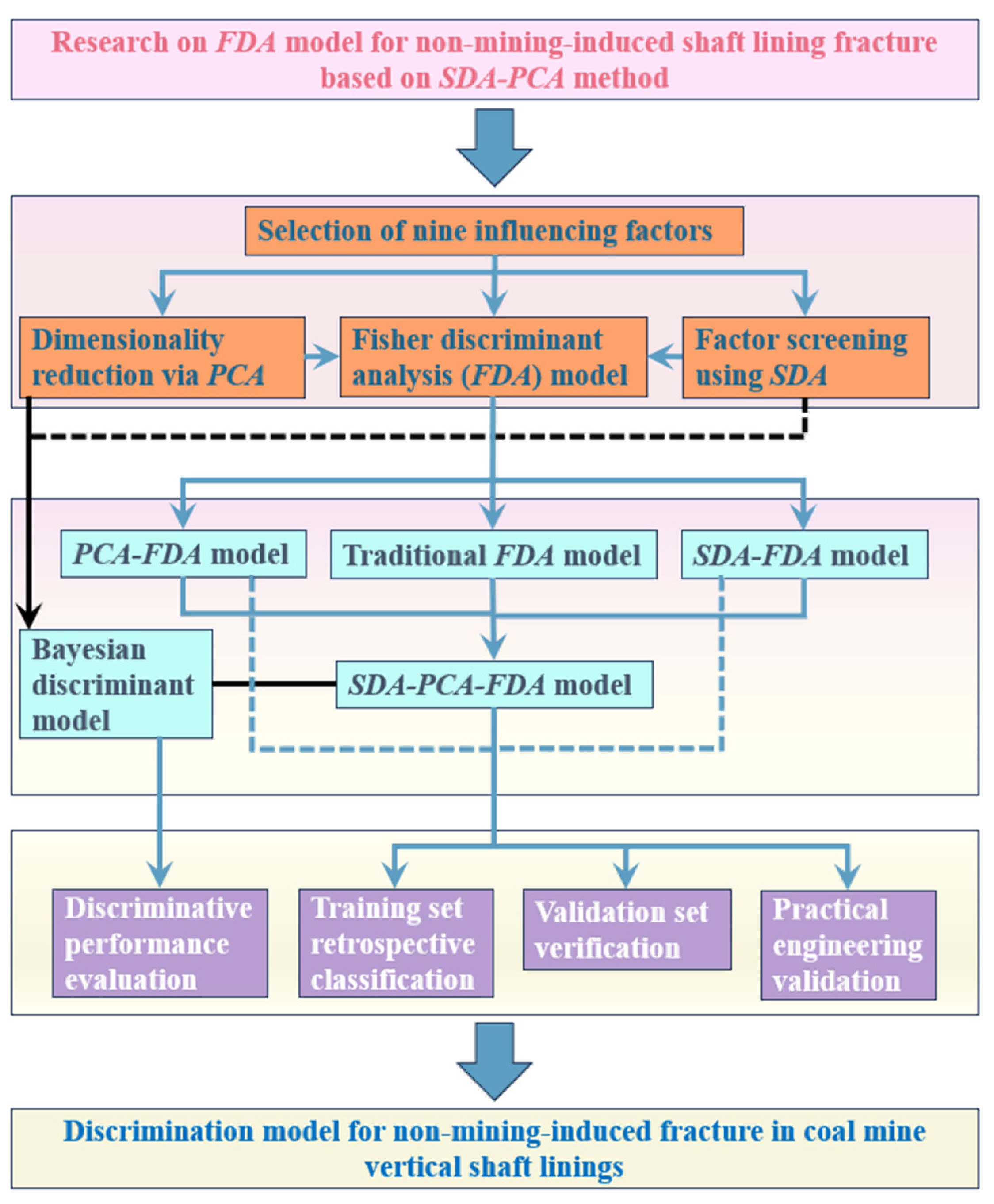
Figure 1. Research roadmap of discriminant analysis model for non-mining fracture of shaft.
Processes 13 04016 g001
Figure 2. Correct classification rates of different models on the training and testing sets.
Processes 13 04016 g002
Figure 3. Gravel diagram.
Processes 13 04016 g003
Figure 4. Cumulative variance contribution rate.
Processes 13 04016 g004
Figure 5. Schematic diagram of shaft rupture and friction pile method.
Processes 13 04016 g005
Figure 6. The NM2dc computational model.
Processes 13 04016 g006
Figure 7. Contour maps of stratum compression under different stiffness coefficients and pile heights.
Processes 13 04016 g007
Figure 8. Relationship between different stiffness coefficients, friction pile height, and stratum settlement.
Processes 13 04016 g008
Figure 9. Contour maps of stratum compression under different friction pile to shaft wall spacings.
Processes 13 04016 g009
Figure 10. Stratum settlement variation curves with friction pile spacing at different locations.
Processes 13 04016 g010
Figure 11. Verification diagram of measured surface subsidence profile.
Processes 13 04016 g011
Table 1. Discrimination results of training samples and different models of non-mining fracture parts of coal mine shaft in Yanzhou mining area.
Shaft
Sample
Influencing FactorsActual
Condition
Discriminant Result
γ1/mγ2γ3/%γ4/mγ5/mγ6/%γ7γ8/%γ9FDAPCA-FDASDA-FDASDA-PCA-FDASDA-PCA-Bayes
01189.301006.518.325.0050.00RuptureRuptureRuptureRuptureRuptureRupture
02189.51905.517.120.0360.01RuptureNon-rupture *Non-rupture *Non-rupture *Non-rupture *Non-rupture *
03190.40907.522.720.0050.00RuptureRuptureRuptureRuptureRuptureRupture
04176.50905.018.012.0320.01RuptureRuptureRuptureRuptureRuptureRupture
05185.41805.014.330.0250.00RuptureRuptureRuptureRuptureRuptureRupture
06189.301006.514.528.5050.00RuptureRuptureRuptureRuptureRuptureRupture
07190.401007.516.623.3050.00RuptureNon-rupture *Non-rupture *Non-rupture *RuptureRupture
08176.501005.07.8015.2320.00RuptureRuptureRuptureRuptureRuptureRupture
09184.51805.020.018.0250.00RuptureRuptureRuptureRuptureRuptureRupture
10189.30906.59.3010.9141.60Non-ruptureNon-ruptureNon-ruptureNon-ruptureNon-ruptureNon-rupture
11176.50135.02.901.30031.30Non-ruptureNon-ruptureNon-ruptureNon-ruptureNon-ruptureNon-rupture
12189.511005.519.316.8049.90Non-ruptureNon-ruptureNon-ruptureNon-ruptureNon-ruptureNon-rupture
13190.4047.53.701.5041.60Non-ruptureNon-ruptureNon-ruptureNon-ruptureNon-ruptureNon-rupture
14180.911007.513.00.0160.01Non-ruptureRupture *Non-ruptureRupture *Non-ruptureNon-rupture
15189.301006.511.813.8135.80Non-ruptureNon-ruptureNon-ruptureNon-ruptureNon-ruptureNon-rupture
16176.50575.05.101.5036.20Non-ruptureNon-ruptureNon-ruptureNon-ruptureNon-ruptureNon-rupture
17189.511005.520.216.2035.80Non-ruptureRupture *Non-ruptureNon-ruptureNon-ruptureNon-rupture
18190.40417.510.22.6035.80Non-ruptureNon-ruptureNon-ruptureNon-ruptureNon-ruptureNon-rupture
19183.511008.013.02.5160.00Non-ruptureRupture *Rupture *Rupture *Non-ruptureRupture *
20189.511005.526.819.2050.00RuptureRuptureRuptureRuptureRuptureRupture
Note: Samples marked with “*” denote misclassified cases; unlisted shaft samples were all correctly classified and are not enumerated here.
Table 2. The test results of the non-mining fracture part of the coal mine shaft and the discrimination results of different models in Yanzhou mining area.
Shaft
Sample
Influencing FactorsActual
Condition
Discriminant Result
γ1/mγ2γ3/%γ4/mγ5/mγ6/%γ7γ8/%γ9FDAPCA-FDASDA-FDASDA-PCA-FDASDA-PCA-Bayes
01190.401007.513.06.1018.20Non-ruptureRupture *Non-ruptureRupture *Non-ruptureRupture *
02176.40505.08.73.807.30Non-ruptureNon-ruptureNon-ruptureNon-ruptureNon-ruptureNon-rupture
03189.511005.530.220.5218.20RuptureNon-rupture *Non-rupture *RuptureRuptureRupture
04173.411004.520.017.0150.01RuptureRuptureRuptureRuptureRuptureRupture
05176.911006.515.03.0375.00Non-ruptureNon-ruptureNon-ruptureNon-ruptureNon-ruptureRupture *
06157.911004.515.025.0020.00RuptureRuptureRuptureRuptureRuptureRupture
07148.611006.513.525.0050.01RuptureRuptureRuptureRuptureRuptureRupture
08190.401007.510.66.8018.20Non-ruptureRupture *Rupture *Rupture *Rupture *Non-rupture
09176.5088.85.08.02.907.30Non-ruptureNon-ruptureNon-ruptureNon-ruptureNon-ruptureNon-rupture
10189.301006.518.517.2118.20RuptureNon-rupture *RuptureRuptureRuptureRupture
Note: Samples marked with “*” denote misclassified cases; unlisted shaft samples were all correctly classified and are not enumerated here.
Table 3. Collinear statistics.
VariableToleranceVIFDimensionEigenvalueCondition Index
(Constant)--16.7061.000
γ20.2494.00821.0992.471
γ30.4082.45130.5273.569
γ40.3662.72940.3844.181
γ50.2693.72050.1746.211
γ60.2194.56960.06110.490
γ70.2883.47570.03413.978
γ80.2354.25780.01125.103
γ90.3283.04890.00633.940
Table 4. Explanation of total variance.
Principal
Component
EigenvalueVariance Contribution Rate/%Cumulative Variance Contribution Rate/%
13.59239.91439.914
22.58828.75068.664
31.84720.52589.189
40.4424.90994.098
50.2622.91597.013
60.1791.98598.998
70.0860.95999.957
80.0030.03399.990
90.0010.010100.000
Table 5. Component coefficient matrix.
Principal Component Y1Principal Component Y2Principal Component Y3
γ10.148−0.2390.375
γ20.0960.3110.022
γ30.327−0.0140.021
γ4−0.0960.0260.537
γ50.397−0.0590.046
γ60.388−0.129−0.126
γ70.0070.249−0.042
γ8−0.0530.3670.430
γ9−0.1420.429−0.032
Table 6. Wilks’ Lambda.
Test of FunctionWilksLambdaChi-Square TestSignificance
y 0.28061.0160.000
Table 7. The accuracy of discriminant models based on different methods.
Discriminant ModelCorrect Classification Rate/%
Training SetTesting Set
FDA82.1466.67
PCA-FDA89.2983.33
SDA-FDA85.7183.33
SDA-PCA-FDA96.4391.76
SDA-PCA-Bayes92.8683.33
Table 8. Evaluation of the safety status of each shaft in a mine.
Shaft Nameγ1/mγ5/mγ6/%γ7γ8/%PC1PC2PC3y-ValuePredicted Result
Main shaft189.318.617.3131.30.5230.530−0.193−0.658Rupture
Auxiliary shaft190.410.26.8018.2−1.645−0.137−0.5752.064Non-rupture
East air shaft176.48.32.607.5−0.9671.522−0.1312.301Non-rupture
Table 9. Summary of rock strata thickness and relevant parameters for numerical simulation.
LithologyDepth/mDensity
/(g·cm−1)
KKurRfCφΔφK0KnsKvs
Topsoil31.862003000.63223.20.670.000210.00021
Medium coarse sand82.23004500.63223.20.670.000210.00021
Medium coarse sand132.23004500.63223.20.670.000210.00021
Sandy clay1082.24006000.70301.30.40.01610.0161
Sandy clay1252.24006000.70301.30.40.01610.0161
Coarse sand Gravel1482.15007500.632211.70.670.000210.00021
Coarse sand Gravel1562.15007500.632211.70.670.000210.00021
sandy clay1962.14306450.60301.30.40.0530.053
Sandy clay2062.14306450.60301.30.40.0530.053
Medium sand2102.170010500.70303.20.42.5362.536
Medium sand2142.170010500.70303.20.42.5362.536
Clay2282.280012000.7522170.60.000210.00021
Clay2312.280012000.7522170.60.000210.00021
Table 10. Research schemes for friction pile height and stiffness.
Scheme
Category
SchemeFriction Pile
Coordinates
Friction Pile Height (m)Stiffness
Coefficient
Dewatering Point
Coordinates
Horizontal schemes Scheme 1 (0, 0)~(0, 112.86)112.860.5(0, 7)
Scheme 2 (0, 0)~(0, 112.86)112.860.1(0, 7)
Scheme 3 (0, 0)~(0, 112.86)112.860.9(0, 7)
Vertical schemes Scheme 4 (0, 0)~(0, 49.86)49.860.5(0, 7)
Scheme 5 (0, 0)~(0, 235.73)235.730.5(0, 7)
Table 11. Calculation of influence percentage for different schemes.
SchemeFriction Pile Height (m)Stiffness
Coefficient
Stable Settlement at Failure Point (m)Settlement at 1 m Radial Distance from Pile (m)Reduction Percentage
Scheme 1 112.860.50.1710.11830.9%
Scheme 2 112.860.10.1630.11728.2%
Scheme 3 112.860.90.1790.12331.3%
Scheme 4 49.860.50.1580.12819.0%
Scheme 5 235.730.50.1900.13827.4%
Table 12. Simulation schemes for friction pile to shaft wall spacing.
SchemeFriction Pile
Presence
Distance from
Pile to Shaft (m)
Friction Pile
Height (m)
Stiffness
Coefficient
Dewatering Point Coordinates
Scheme 1 Yes5112.860.9(0, 7)
Scheme 2 Yes10112.860.9(0, 7)
Scheme 3 Yes15112.860.9(0, 7)
Scheme 4 No//0.9(0, 7)
Table 13. Influence of friction piles on the shaft wall.
SchemeFriction Pile Height/mDistance from Shaft to Pile/mStable Settlement at Failure Point/mSettlement at 1 m from Shaft Wall/mReduction
Percentage
Scheme 1 112.8650.1500.00795.3%
Scheme 2 112.86100.1500.00696.0%
Scheme 3 112.86150.1500.00994.0%
Table 14. Costs of different shaft governance schemes (Unit: ×104 CNY).
ItemScheme 1Scheme 2Scheme 3Scheme 4Scheme 5
Construction preparation2020202020
Surface grouting///600/
Wall-penetrating grouting6040///
Relief groove construction151515//
Shaft ring reinforcement//3030/
Shaft equipment modification55555
Friction pile construction////450
Monitoring instrumentation cost2020202020
Engineering design2010103030
Project close-out22222
Total cost142112102697517
Duration/days555020150140
Table 15. Analysis of advantages and disadvantages of different shaft governance schemes.
SchemeContentAdvantagesDisadvantages
Scheme 1 Chemical grouting at 213 m~230 m depth + relief groove at 223 m depthEffective pressure relief on the shaft wall; good water-plugging effect from groutingCertain risk associated with creating the relief groove; requires a construction cycle inside the shaft; high cost of chemical materials; high requirements for process and material mix
Scheme 2 Cement grouting at 213 m~230 m depth + relief groove at 223 m depthEffective pressure relief on the shaft wall; relatively low costCertain risk associated with creating the relief groove; requires a construction cycle inside the shaft; poor water-plugging effect from grouting
Scheme 3 Shaft ring reinforcement at 213 m~230 m depth + relief groove at 223 m depthShort construction period; can quickly control the development of failureShort duration of protective effect; certain safety risks exist
Scheme 4 Surface grouting to reinforce the loose stratum + shaft ring reinforcementMinimal construction work inside the shaft; large grouting rangePoor effectiveness in reducing additional stress; high cost and material mix requirements
Scheme 5 Friction pile method at 10 m from the shaft wallNo internal shaft construction required; high shaft protection effectiveness; high safetyHigh process requirements; high cost
Disclaimer/Publisher’s Note: The statements, opinions and data contained in all publications are solely those of the individual author(s) and contributor(s) and not of MDPI and/or the editor(s). MDPI and/or the editor(s) disclaim responsibility for any injury to people or property resulting from any ideas, methods, instructions or products referred to in the content.