Performance Improvement of Photovoltaic Panels Through Advanced Fault Detection Techniques

Abstract

Early detection of performance degradation and prevention of critical failures in photovoltaic (PV) arrays are essential for ensuring system reliability and efficiency. This study presents an intelligent fault detection and classification framework based on a Multi-Layer Neural Network (MLNN). The model was developed and validated using a simulated 250 kW grid-connected PV system tested under five operating scenarios: normal operation, open-circuit fault, partial short-circuit, partial shading, and string-to-string fault. Unlike conventional diagnostic approaches, the proposed model directly processes raw electrical measurements (current, voltage, power, irradiance, and temperature) under varying environmental conditions, thus emulating real-world operational variability. The MLNN achieved 98% test accuracy and outperformed benchmark classifiers Support Vector Machine (SVM) and Random Forest (RF) across multiple metrics. Performance was evaluated using the confusion matrix, precision, recall (sensitivity) and F1-score. The framework is designed for scalability and can be integrated into predictive maintenance platforms to enable early fault detection and improve long-term PV system availability and efficiency.

1. Introduction

The growing global demand for PV systems as a sustainable and clean energy source has highlighted the importance of ensuring their operational reliability and long-term efficiency [1,2]. Despite offering substantial environmental and economic advantages, PV systems are inherently susceptible to various faults such as open-circuit faults, partial short circuits, partial shading, and string-to-string mismatches. These faults can cause significant power losses and, in severe cases, may even pose safety hazards like electrical arcing or fire [2]. Conventional fault detection techniques such as manual inspections, infrared thermography, and I–V curve tracing have proven inadequate, especially in utility-scale PV installations. These methods are often labor-intensive, lack sensitivity to early stage or internal faults, and are incapable of providing real-time diagnostics [3,4,5]. To overcome these limitations, intelligent Fault Detection and Diagnosis (FDD) systems based on data driven approaches have gained increasing attention in recent years. Among various machine learning and artificial intelligence methods, Artificial Neural Networks (ANNs) have emerged as powerful tools due to their ability to learn complex non-linear patterns, adapt to noisy and uncertain inputs, and generalize across different operational environments [6,7,8,9]. Specifically (MLNNs) have demonstrated high effectiveness in recognizing subtle fault signatures in PV systems [10]. In this context, this study introduces an MLNN-based fault classification framework designed and implemented for a 250 kW grid-connected PV system simulated in MATLAB/Simulink (R2022b). The system is simulated under five representative operating conditions: normal operation, open-circuit fault, partial short-circuit, partial shading, and string-to-string fault. Unlike many previous studies that rely on engineered statistical features or small-scale datasets, this work employs raw signal data including voltage, current, power, irradiance, and temperature captured under varying environmental conditions to enhance realism and robustness. Moreover, the modular design of the proposed model provides a foundation for future integration with predictive fault diagnosis techniques, enabling proactive maintenance strategies. Consequently, the framework is suitable not only for current fault detection tasks but also scalable toward predictive analytics in real- time PV monitoring systems.

In recent years substantial research efforts have been directed toward the development of intelligent Fault Detection and Diagnosis (FDD) techniques for PV systems. Conventional methods such as I–V curve analysis, infrared thermography, and manual inspections have proven largely inadequate for large scale PV installations due to their limited scalability, inability to detect internal or incipient faults, and lack of real time responsiveness [3,4,5]. These limitations have prompted a growing shift toward Machine Learning (ML) and Artificial Intelligence (AI)-based solutions, which offer superior diagnostic accuracy, automation, and adaptability. Among AI methods, ANNs have gained prominence in PV fault diagnostics owing to their capacity to learn from historical data and identify complex, non-linear fault patterns. Chine et al. [11] introduced an ANN-based model that achieved high classification accuracy across several fault types. Similarly, Mellit et al. [6] employed feedforward neural networks, reporting notable improvements in fault detection performance. To further improve robustness and adaptability, hybrid approaches have also been explored, integrating ANNs with adaptive algorithms and real time monitoring systems. For example, Sepúlveda-Oviedo et al. [9] combined AI-based algorithms with monitoring frameworks for enhanced real- time diagnostics, while Abubakar et al. [8] surveyed ANN-based hybrid frameworks for increased reliability. Additionally, other ML techniques such as SVM and Deep Learning architectures [12] have been investigated for their potential in PV fault classification. However, despite notable progress, several challenges remain unresolved. Many existing models exhibit poor generalization under variable environmental conditions or degraded performance in the presence of noisy inputs [13,14]. Moreover, a considerable proportion of the literature focuses on fault detection only after the event has occurred, offering limited predictive insights that could enable proactive maintenance strategies.

Table 1 summarizes the most relevant studies related to PV fault detection and classification. It highlights the systems, methods, limitations, and performance outcomes reported in the literature. As observed, most existing studies focused on small-scale systems or limited fault types, while the proposed framework in this study addresses these gaps through a 250 kW large-scale model, randomized fault scenarios.

This study aims to improve the precision and reliability of fault detection in PV systems by addressing the shortcomings identified in earlier research. A modular classification framework based on an MLNN is developed, utilizing raw electrical measurements current, voltage, power, irradiance, and temperature across varying environmental conditions. The central research question addressed is whether a data-driven MLNN trained on raw signals can achieve more accurate and robust fault classification than conventional diagnostic approaches. However, previous studies have primarily focused on small-scale PV systems or relied on engineered statistical features, limiting their scalability and generalization capability. To address these gaps, the present study makes the following key contributions:

• A detailed 250 kW grid-connected PV system is developed using a modular, string-level configuration, providing higher scale and resolution than most existing studies (typically below 10 kW).
• The proposed framework utilizes raw electrical signals instead of preprocessed or statistical features, enabling a richer and more flexible feature space for model training.
• The system is evaluated under diverse irradiance and temperature conditions, ensuring robustness and generalizability of the results.
• A comprehensive comparative analysis of three ML algorithms MLNN, SVM, and RF is performed on a unified dataset to guarantee consistency and fairness in benchmarking [15,16,17].
• The proposed MLNN model achieves a test accuracy of 98%, ranking among the highest reported performances in simulation-based PV fault classification studies [18].

Table 1. Summary of previous studies on PV fault detection.

References	System Used	Methodology	Limitations	Outcomes of Study
Mellit et al., 2018 [2]	Various PV systems (review)	Surveyed fault detection and diagnosis (FDD) methods including I–V curve tracing, ANN, and SVM approaches	No unified test platform; lacked environmental variability and ML implementation details	Identified the need for adaptive, data-driven diagnostic models for large-scale PV arrays
Ghoneim et al., 2021 [5]	PV farm (MATLAB/Simulink)	Rule-based fault detection algorithms for maintaining service continuity	Sensitive to sensor errors; limited scalability for large systems	Achieved 85–90% accuracy under ideal conditions; failed under noisy data
Mellit & Kalogirou, 2022 [6]	5 kW PV array simulation	Comparative study using ANN, SVM, and RF classifiers	Fixed fault locations; no cross-validation; narrow irradiance range	RF achieved 92% accuracy; ANN showed better generalization ability
Li et al., 2021 [7]	PV array (review)	Reviewed ANN-based FDD approaches	Focused on ANN only; ignored hybrid and ensemble approaches	Highlighted ANN’s effectiveness but noted limited robustness to noise
Patthi et al., 2024 [3]	PV string (Simulink)	Multi-Layer Neural Network (MLNN)-based optimization	Single fault case; no irradiance variability	MLNN reached 95% accuracy; limited dataset diversity
Amiri et al., 2024 [17]	Real PV plant data	Random Forest classifier for fault detection	Pre-processing steps and noise robustness not specified	RF achieved 91% accuracy; model performed well but lacked environmental validation
Liu & Wu, 2025 [12]	PV module datasets (review)	Deep learning-based fault detection survey	Theoretical study; no experimental verification	Highlighted the lack of reproducible datasets and standardized evaluation metrics
Proposed work	250 kW grid-connected PV system (MATLAB/Simulink)	MLNN-based framework with randomized fault locations, variable irradiance–temperature, and cross-validation	Previous works lacked randomized faults, and detailed pre-processing	Achieved 98% accuracy, and reproducibility under diverse environmental conditions

Table 1. Summary of previous studies on PV fault detection.

References	System Used	Methodology	Limitations	Outcomes of Study
Mellit et al., 2018 [2]	Various PV systems (review)	Surveyed fault detection and diagnosis (FDD) methods including I–V curve tracing, ANN, and SVM approaches	No unified test platform; lacked environmental variability and ML implementation details	Identified the need for adaptive, data-driven diagnostic models for large-scale PV arrays
Ghoneim et al., 2021 [5]	PV farm (MATLAB/Simulink)	Rule-based fault detection algorithms for maintaining service continuity	Sensitive to sensor errors; limited scalability for large systems	Achieved 85–90% accuracy under ideal conditions; failed under noisy data
Mellit & Kalogirou, 2022 [6]	5 kW PV array simulation	Comparative study using ANN, SVM, and RF classifiers	Fixed fault locations; no cross-validation; narrow irradiance range	RF achieved 92% accuracy; ANN showed better generalization ability
Li et al., 2021 [7]	PV array (review)	Reviewed ANN-based FDD approaches	Focused on ANN only; ignored hybrid and ensemble approaches	Highlighted ANN’s effectiveness but noted limited robustness to noise
Patthi et al., 2024 [3]	PV string (Simulink)	Multi-Layer Neural Network (MLNN)-based optimization	Single fault case; no irradiance variability	MLNN reached 95% accuracy; limited dataset diversity
Amiri et al., 2024 [17]	Real PV plant data	Random Forest classifier for fault detection	Pre-processing steps and noise robustness not specified	RF achieved 91% accuracy; model performed well but lacked environmental validation
Liu & Wu, 2025 [12]	PV module datasets (review)	Deep learning-based fault detection survey	Theoretical study; no experimental verification	Highlighted the lack of reproducible datasets and standardized evaluation metrics
Proposed work	250 kW grid-connected PV system (MATLAB/Simulink)	MLNN-based framework with randomized fault locations, variable irradiance–temperature, and cross-validation	Previous works lacked randomized faults, and detailed pre-processing	Achieved 98% accuracy, and reproducibility under diverse environmental conditions

Collectively, these contributions advance the development of robust and scalable fault detection and diagnosis (FDD) frameworks, forming a solid foundation for future research on predictive fault diagnosis and real-time monitoring applications.

The structure of this study is organized as follows:

Section 2 describes the overall configuration of the PV system under investigation. Section 3 provides an overview of the PV system and summarizes the key parameters used in the simulation study.

Section 4 defines and categorizes the different types of faults considered in this work. Section 5 introduces the machine learning-based fault classification approach and briefly explains the employed algorithms.

Section 6 outlines the adopted methodology, including data generation, preprocessing, model training, and evaluation procedures.

Section 7 presents and discusses the obtained results, highlighting the comparative performance of the proposed models.

Section 8 provides the main conclusions drawn from this study.

Finally, Section 9 discusses the study’s limitations and proposes directions for future research.

2. System Description

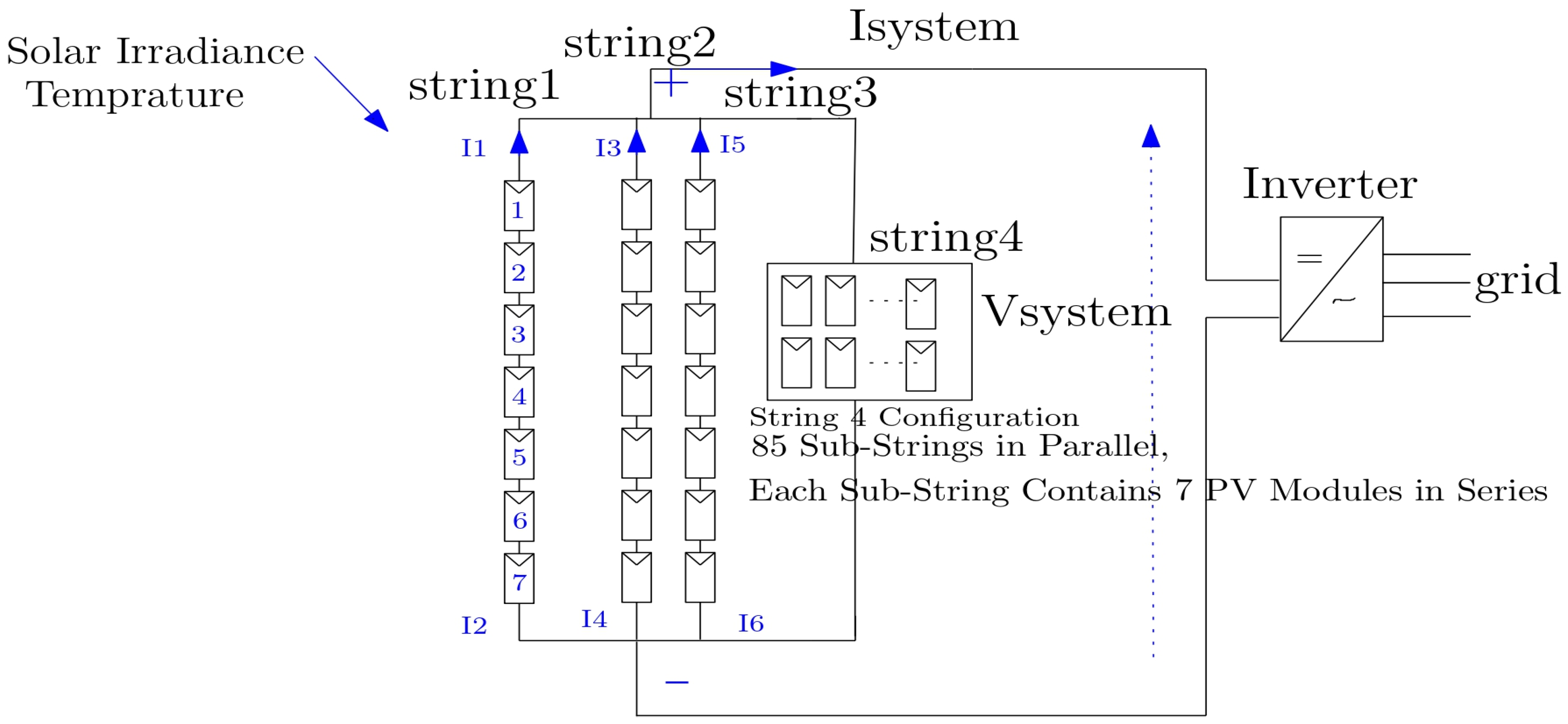
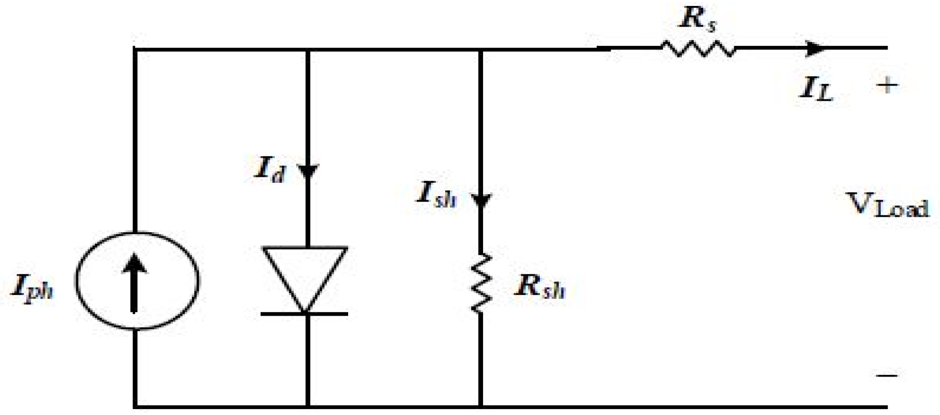
The overall PV system was developed in MATLAB/Simulink, where the main block represents a subsystem that encapsulates the entire 250 kW array. The system comprises four main string groups: the first three groups each contain a single series-connected string of seven SunPower SPR-415E-WHT-D modules, while the fourth group includes 85 parallel strings, each formed by seven series-connected modules. In total, the complete array contains 88 strings, yielding a rated capacity of 250 kW. This modular configuration facilitates precise fault injection and measurement at both the string and module levels, while maintaining a clear and well-organized top-level schematic. All four strings are connected in parallel to form the overall PV array. The total output voltage of the system is approximately 510.3 V (7 × Vmp), while the total output current is around 500.72 A, resulting in an estimated power output of 255.5 kW. This modular configuration supports the simulation of realistic fault conditions and enables the generation of labeled voltage and power data. The extracted data were subsequently utilized to train and evaluate fault detection models based on ANN. The electrical behavior of the PV module is represented by the widely adopted one-diode equivalent circuit, as illustrated in Figure 1. The output of the PV array is connected to a three-level IGBT inverter, followed by a step-up transformer (TR1), which adjusts the voltage to match grid requirements. The system is then interfaced with the utility grid and monitored using a power analyzer (P&O) to observe real-time voltage, current, and power characteristics [19,20]. This complete setup enables the evaluation of system dynamics under various operating and fault conditions, thereby facilitating accurate data acquisition for fault classification. The current ${\mathrm{I}}_{\mathrm{L}}$ delivered by the solar cell can accordingly be expressed as follows:

$${\mathrm{I}}_{\mathrm{L}}={\mathrm{I}}_{\mathrm{p}\mathrm{h}}-{\mathrm{I}}_{\mathrm{s}}⌈{\mathrm{e}}^{{\displaystyle \frac{\mathrm{V}+{\mathrm{R}}_{\mathrm{s}}{\mathrm{I}}_{\mathrm{L}}}{\mathrm{n}{\mathrm{V}}_{\mathrm{t}}}}}-1⌉-{\displaystyle \frac{\mathrm{V}{+\mathrm{R}}_{\mathrm{s}}{\mathrm{I}}_{\mathrm{L}}}{{\mathrm{R}}_{\mathrm{s}\mathrm{h}}}}$$

(1)

$$\mathrm{w}\mathrm{h}\mathrm{e}\mathrm{r}\mathrm{e} {\mathrm{V}}_{\mathrm{t}}={\displaystyle \frac{{\mathrm{T}}_{\mathrm{c}}\mathrm{K}}{\mathrm{q}}},\mathrm{K}=1.38\times {\displaystyle \frac{{10}^{-23}\mathrm{J}}{\mathrm{K}}},\mathrm{q}=1.6\times {10}^{-19}\mathrm{C}$$

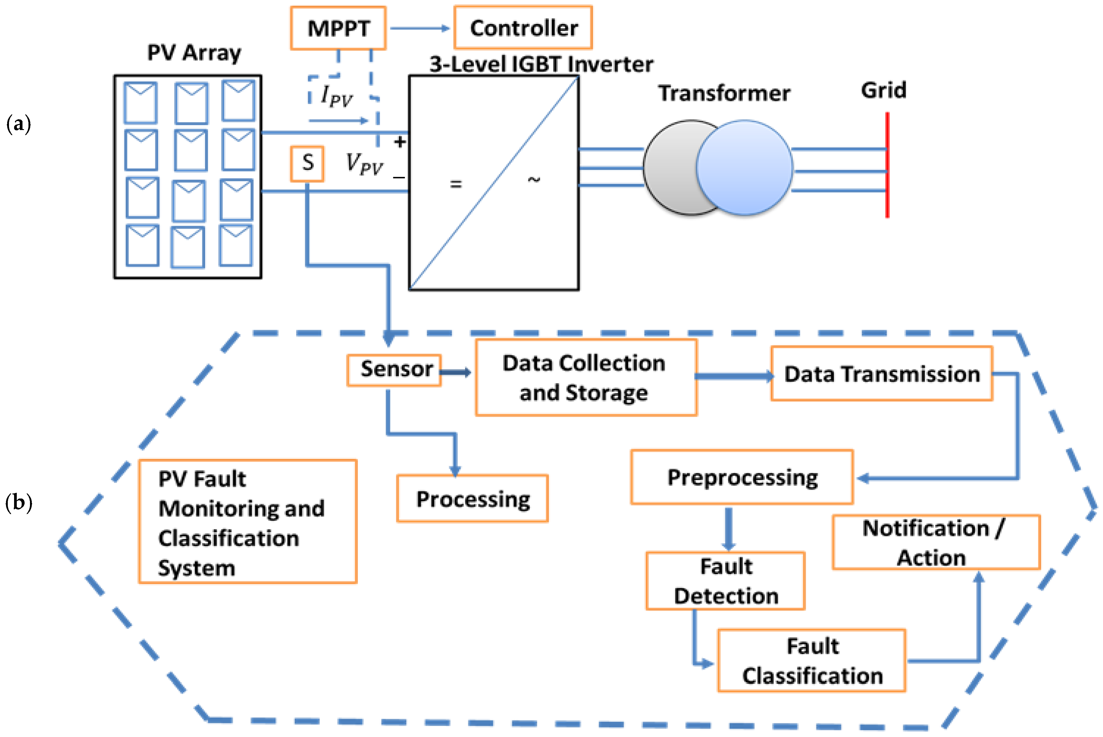
Figure 2 presents the overall architecture of the proposed PV fault monitoring and classification system. Sub-figure (a) illustrates the power conversion section, where the PV array is connected to the MPPT and controller that regulate the inverter and transformer before grid connection. Sub-figure (b) shows the data-driven fault detection framework, which includes data acquisition, preprocessing, fault detection, classification, and notification. Measured electrical and environmental parameters (current, voltage, power, irradiance, and temperature) are processed to identify abnormal operating conditions and trigger corrective actions when faults occur.

3. System Overview and Key Parameters

A comprehensive Simulink model of a 250 kW grid-connected PV system [5] was created in order to assess how the system would behave under the previously described fault types. The system is made up of several parallel PV strings that are interfaced with the grid via a step-up transformer, RL filter, and three-phase inverter. The main PV module and inverter parameters that were entered into the simulation model are compiled in

Table 2. PV module and inverter parameters used in the Simulink model.

Parameter	Value/Type
PV module type	SunPower SPR-415E-WHT-D
Maximum Power Output (Pmax)	414.8 W
Open-Circuit Voltage (Voc)	85.3 V
Short-Circuit Current (Isc)	6.09 A
Voltage at Maximum Power Point (Vmp)	72.9 V
Current at Maximum Power Point (Imp)	5.69 A
Temperature coefficient of Voc (%/deg.C)	−0.229%/°C
Temperature coefficient of Isc (%/deg.C)	0.030706%/°C
Series resistance (Rs)	0.537 Ω
Shunt resistance Rsh	419.8
Diode ideality factor n	0.872
Parallel strings	88
Series-connected modules per string	7
Irradiance profile G(t)	400–1000 W/m2
Temperature profile T(t)	25–45 °C
Parray = 88 × 7 × 414.8 W	255.5 kW
Inverter
Nominal power Pnom	250 kVA
DC-link voltage Vdc	480 V
DC-link capacitance (Clink)	0.0543 F
Grid frequency	50 Hz
Modulation index (m)	0.85

. These settings guarantee practical performance in line with large-scale PV systems.

The irradiance varied between 400–1000 W/m² and the cell temperature between 25–45 °C for all simulated scenarios. These ranges were applied through external inputs to the PV array block to ensure reproducibility.

4. Fault Types Analysis and Definitions

PV systems are inherently susceptible to various fault conditions that can significantly reduce energy yield, degrade overall performance, and, in some cases, pose potential safety hazards if left undetected. These faults are generally categorized into three main groups:

• Electrical faults, such as open-circuit and short-circuit conditions.
• Environmental faults including partial shading, dust accumulation, snow coverage and bird droppings.
• Connection related faults, such as string-to-string mismatches [21,22].

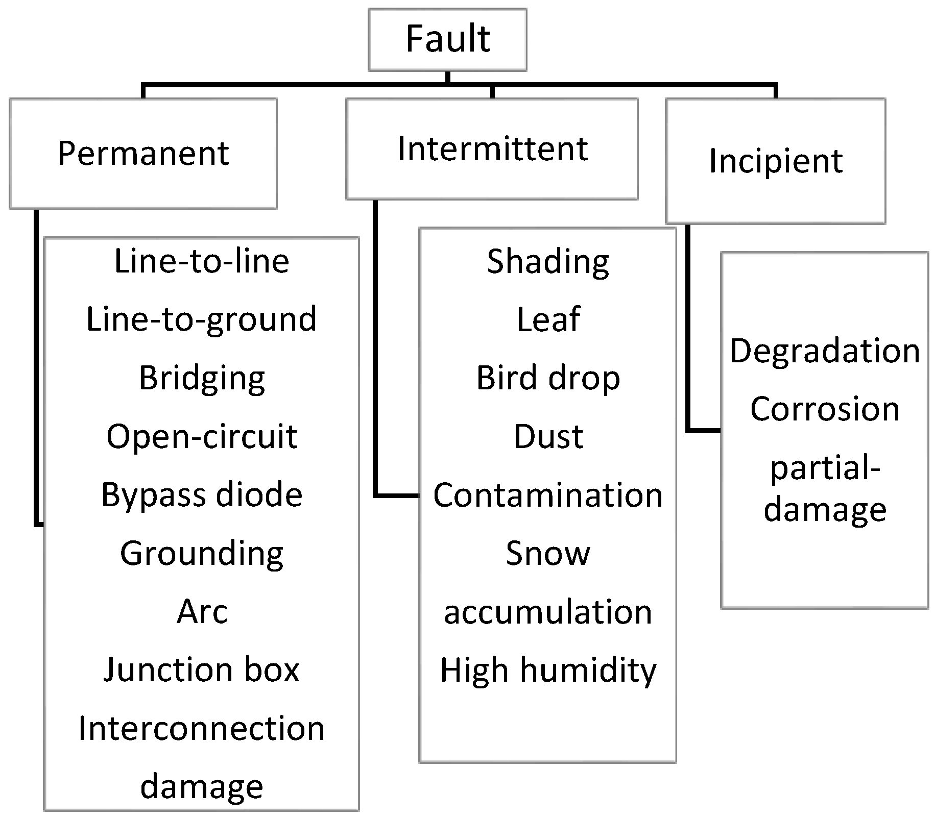
In addition to this functional classification, PV faults can also be grouped based on their temporal behavior into permanent, intermittent, and incipient faults. Intermittent faults are temporary in nature and are typically caused by environmental factors such as shading, contamination, high humidity, or the accumulation of leaves and snow. Permanent faults refer to irreversible damages, including open or short circuits, junction box failures, or interconnection damage. Incipient faults, which often precede permanent faults, result from gradual processes such as cell degradation, corrosion, or partial delamination within the PV module. Such early-stage faults can progressively deteriorate system performance, particularly under conditions of high temperature and humidity. This hierarchical classification is illustrated in Figure 3, providing a comprehensive perspective on how different fault types evolve over time and influence overall system operation [23].

Comparative Analysis of Normal and Fault Operating Conditions in PV System

In order to assess system performance under various fault situations, this study simulated and examined five key operational scenarios for a 250 kW grid-connected PV power plant. These comprise the standard working condition as a reference case, as well as four typical fault types: open-circuit, partial short-circuits, partial shading, and string-to-string faults. To capture its unique effects on the properties of total power, voltage, and current, each situation was meticulously modeled. In order to increase reliability and guarantee continuous energy generation with low losses, the simulations offer important insights into the dynamic behavior of PV systems under actual disturbances. The following sections show the performance differences between faulty and healthy situations by presenting and comparing the outcomes of all operational cases. This methodical assessment highlights the significance of precise and trustworthy fault detection techniques, evaluates the severity of each problem type, and comprehends how it affects overall system performance.

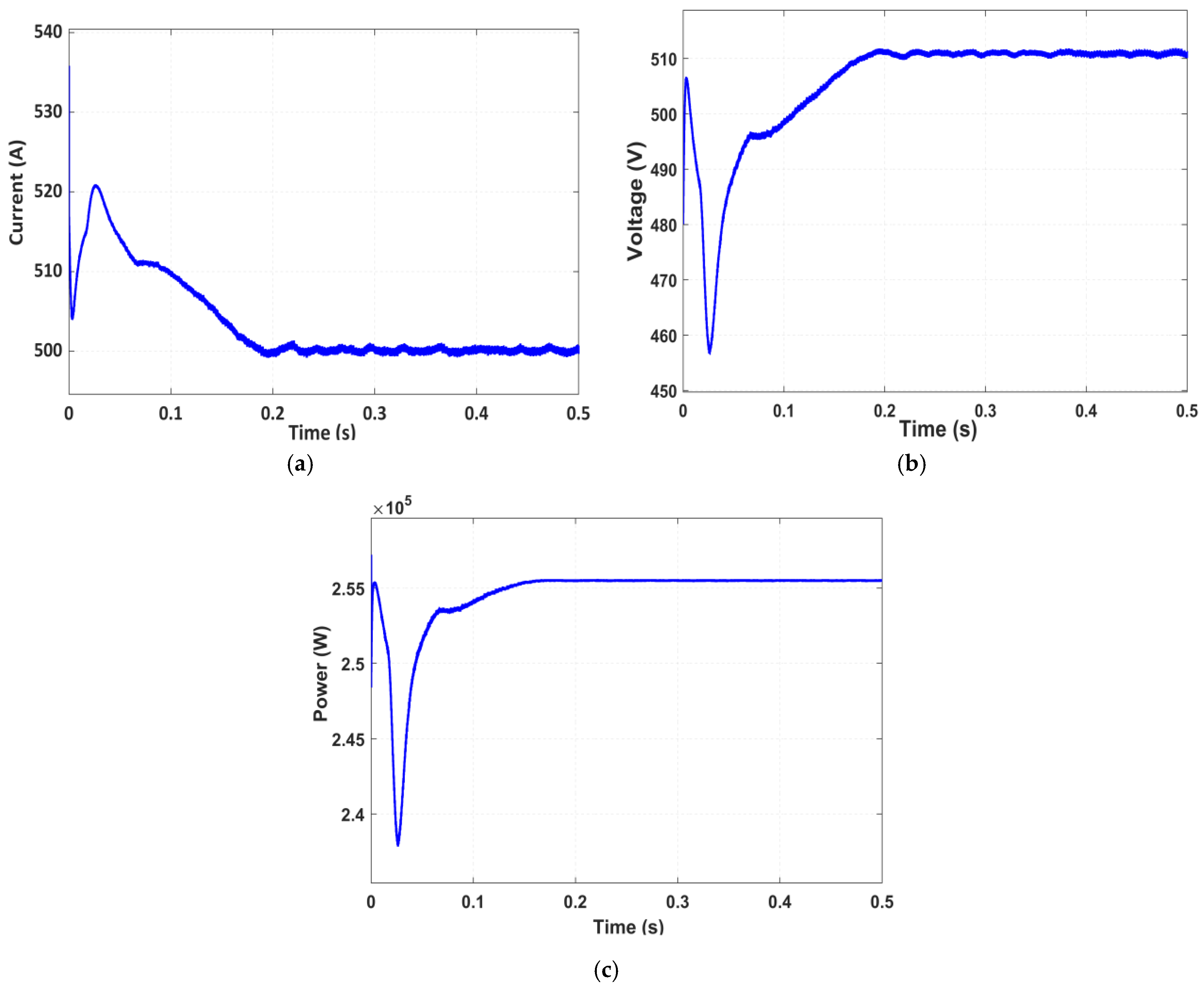
Normal Operation: Figure 4 presents the measured total DC-side current (I System) and voltage (V System) under standard test conditions (irradiance = 1000 W/m² and temperature = 25 °C). Under fault-free conditions, all PV modules operate efficiently within their rated parameters. The system delivers a total current of approximately 500 A, a voltage of 511 V, and a total power output of about 255 kW, which collectively serve as the reference baseline for subsequent fault detection and comparative performance analysis. The corresponding waveforms obtained under normal operation are shown in Figure 5, where sub-figure (a) illustrates the total current, (b) represents the total voltage, and (c) depicts the total power at the DC side. This figure represents a sample from the larger dataset generated under various irradiance and temperature scenarios.

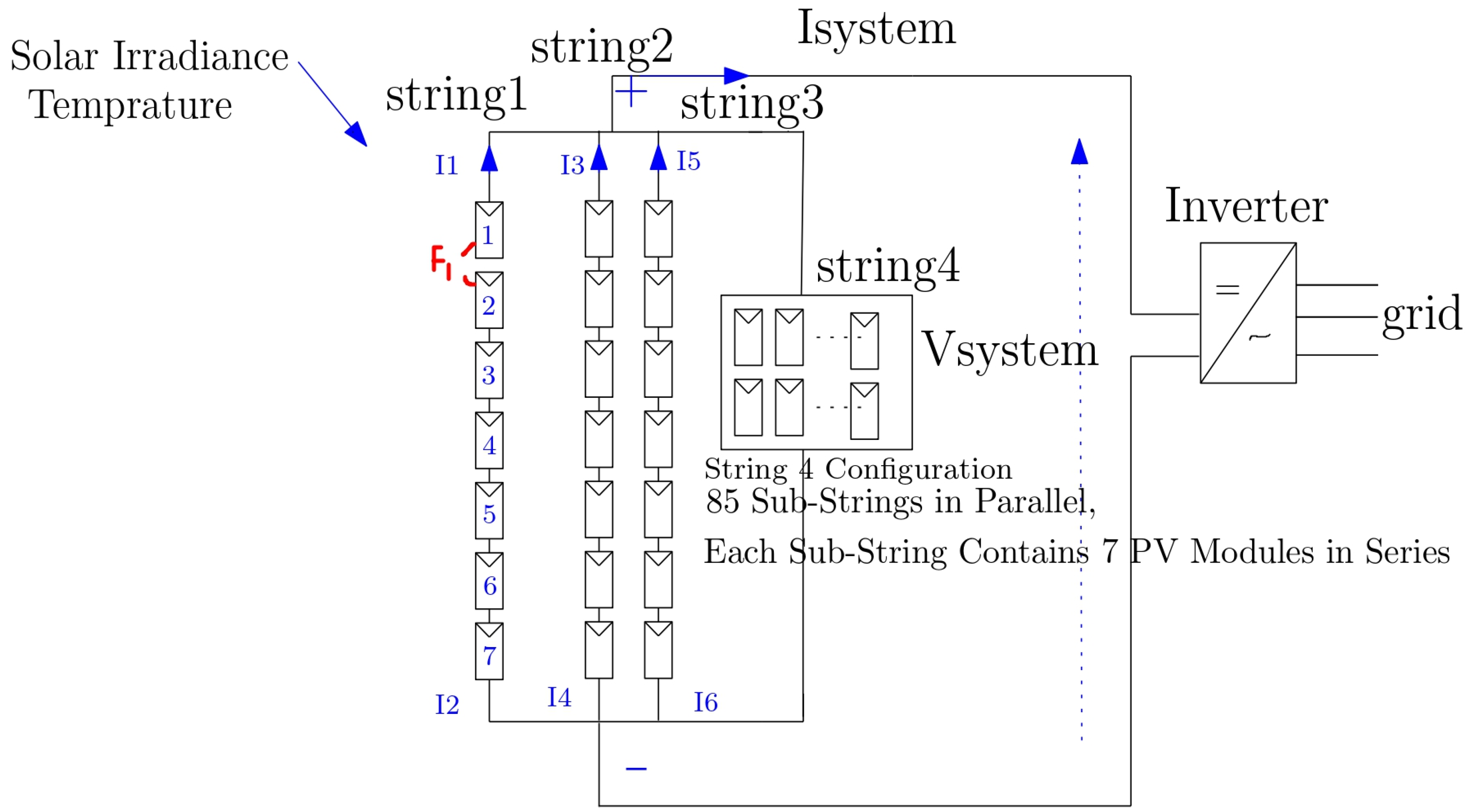
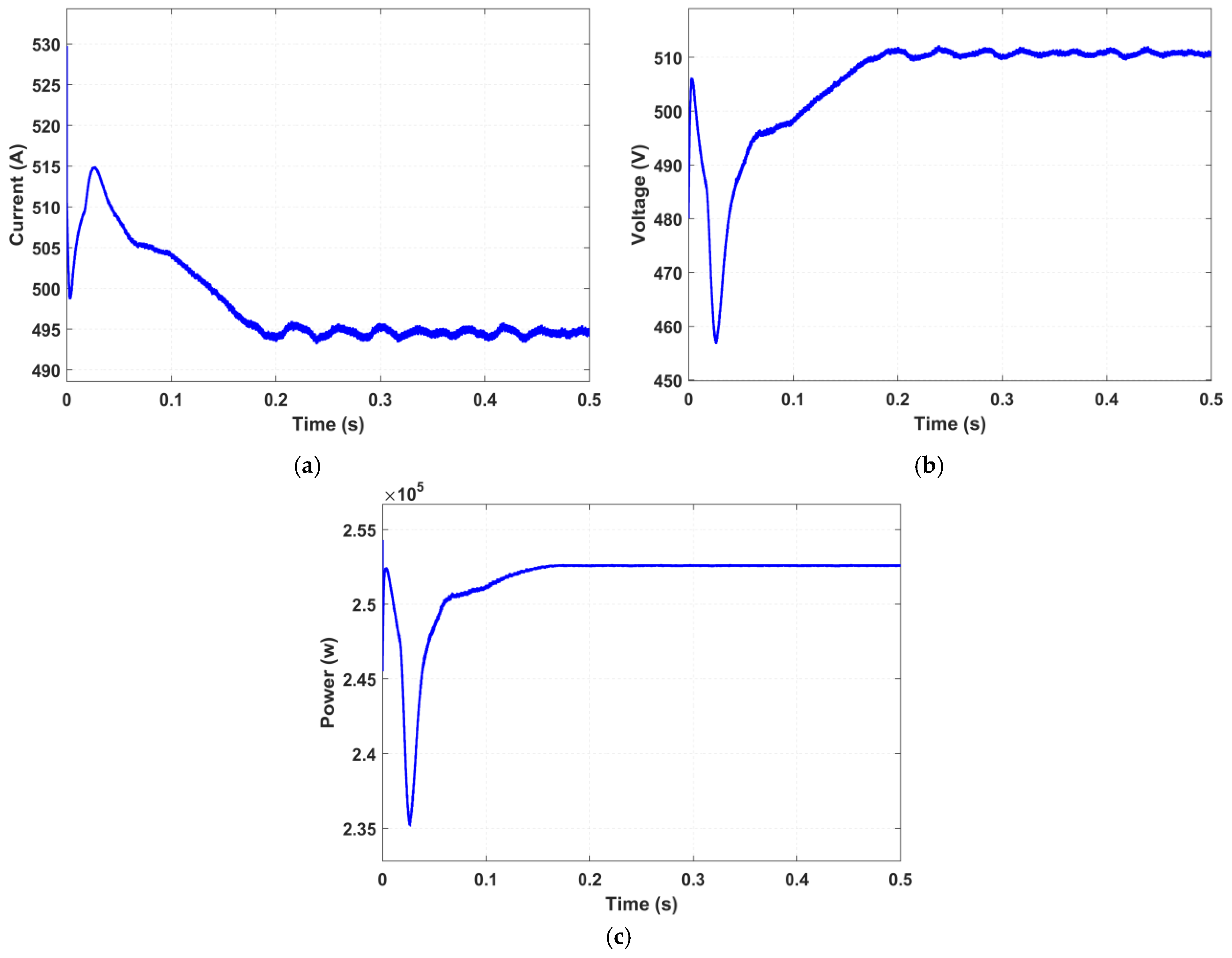
Open-Circuit Fault: Occurs under the simulation conditions (irradiance = 1000 W/m² and temperature = 25 °C) when the electrical continuity within a photovoltaic module or string is interrupted due to connector detachment, solder joint degradation, or broken interconnections. Such interruption prevents the current from flowing through the affected branch, leading to an increase in voltage across the open section and causing a power imbalance among the interconnected strings. In String 1, an open-circuit fault is simulated by cutting the connection between the first and second modules. The current in String 1 (I₁) decreases to zero since there is no current flowing through the open path. As a result, the array current slightly drops to 494.3 A, the overall power output drops to roughly 252 kW, while the total voltage stays almost constant at 511 V. If the fault remains undetected, it may cause uneven stress distribution among modules and affect long-term reliability. Therefore, maintaining optimal system performance requires accurate defect detection. The PV system configuration under this fault is shown in Figure 6, while the variations in total current, voltage, and power at the DC side are illustrated in Figure 7. where sub-figure (a) illustrates the total current, (b) represents the total voltage, and (c) depicts the total power at the DC side.

Partial Short-Circuit Fault: A partial short-circuit fault arises when a low-resistance path forms between two nodes of a module or string, often due to insulation degradation or moisture intrusion. It results in localized heating and reverses current flow, which may accelerate cell damage or cause thermal runaway.

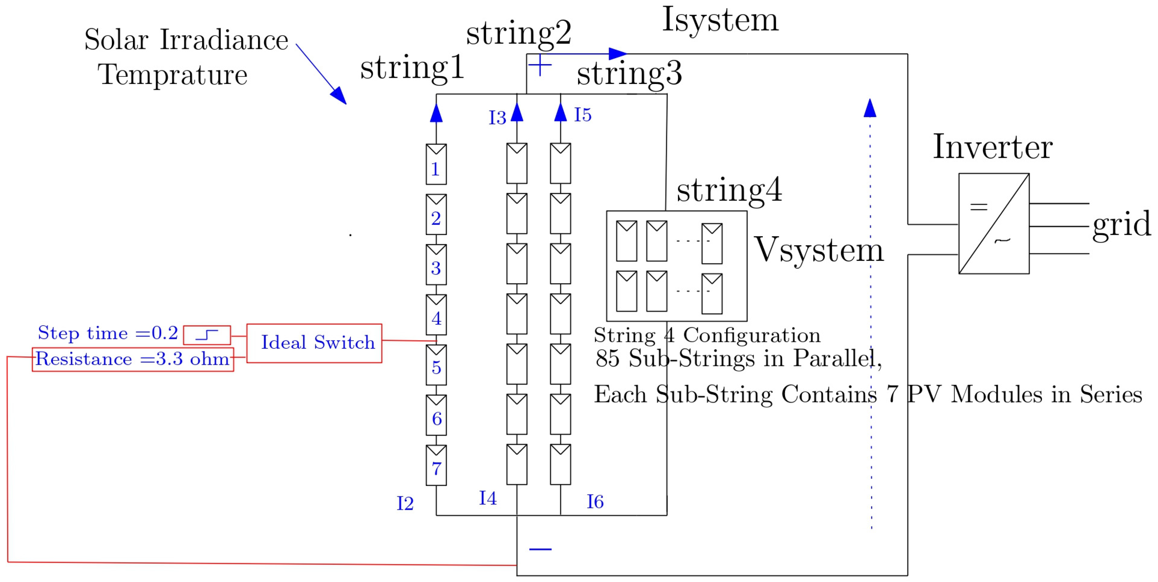
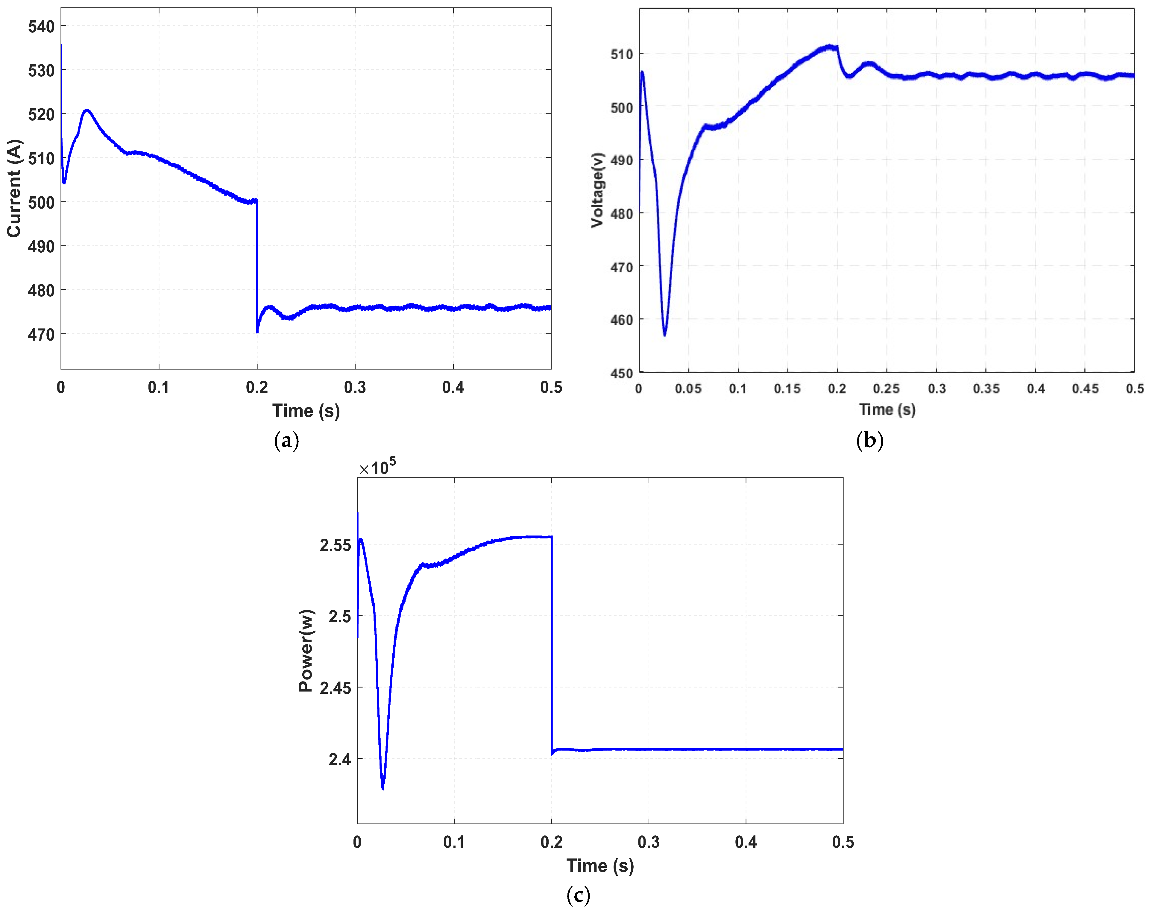
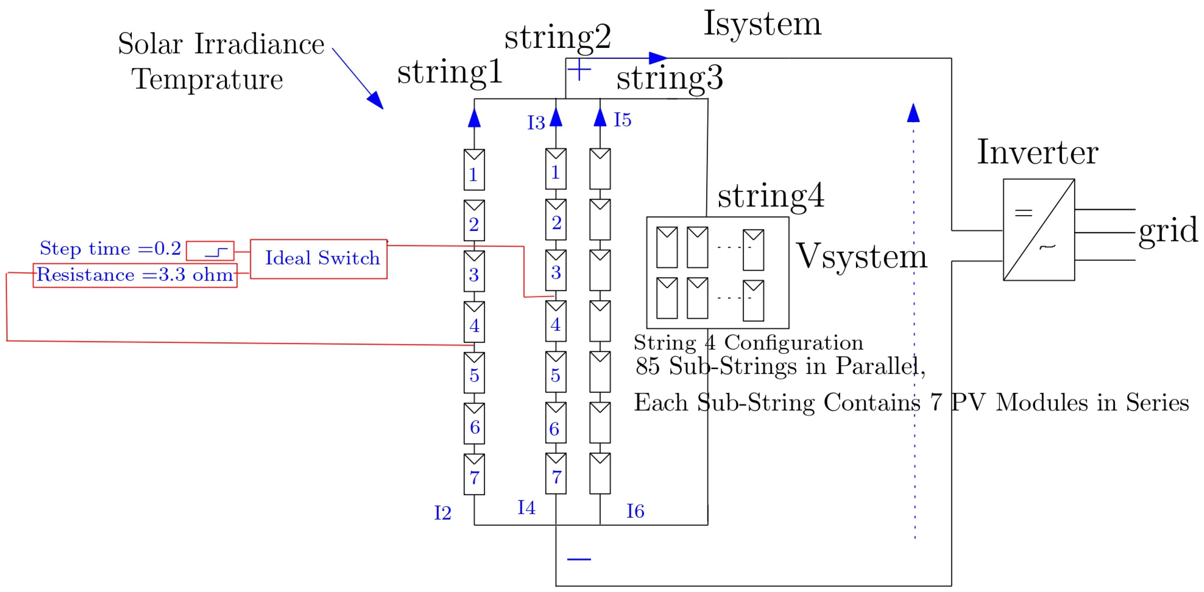
An ideal switch with three terminals is used to model this defect, which is introduced in String 1 between the fourth and fifth modules. A resistor of about 3.3 Ω is connected to terminal 1, and the opposite side of the resistor is grounded. In order to replicate the fault initiation, terminal 2 of the switch is placed between modules 4 and 5, and a step signal is applied to the gate terminal at 0.2 s. Because of internal heating and mismatch effects, a reverse current therefore flows in String 1, lowering the output power to 240 kW, the voltage to 505.9 V, and the overall string current to 475.6 A. Figure 8 displays the PV system layout under this partial short-circuit problem and the variations in total current, voltage, and power at the DC side are presented in Figure 9.

Partial Shading: Occurs when certain modules receive less irradiance due to obstacles such as trees, dust, or debris. The shaded modules produce lower current, causing power mismatch and multiple peaks in the P–V characteristic curve.

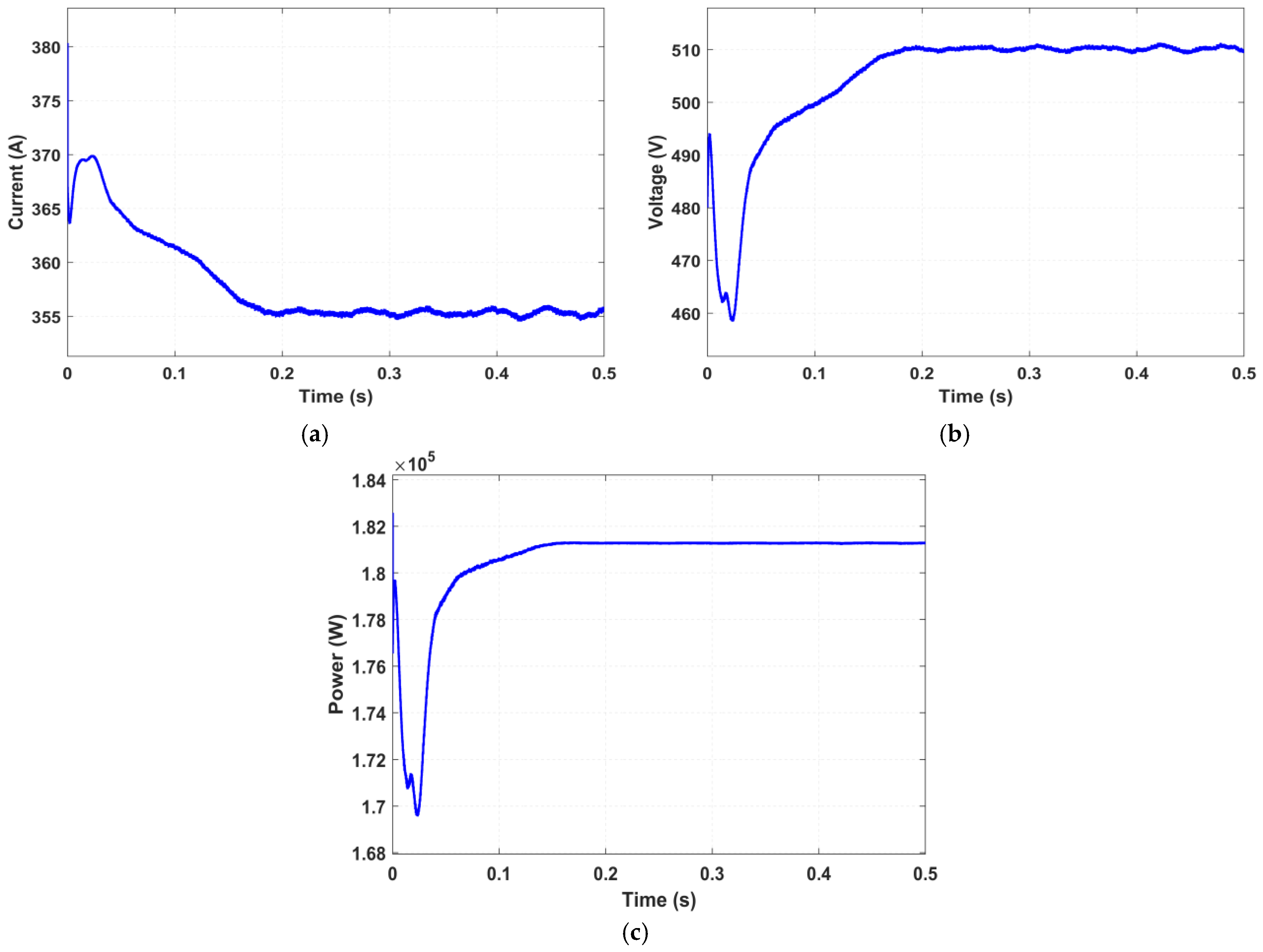
Here, a 30% reduction in irradiance is applied to String 4. As a result, total current drops to 355.6 A, with voltage slightly decreasing to 509.8 V. The power output is severely affected, decreasing to 180 kW, highlighting the impact of mismatch losses, as shown in Figure 10.

String-to-String Fault: This fault is caused by insulation failure between adjacent strings, leading to unintended current exchange paths. It can result in severe imbalance, overheating, or in extreme cases, arcing between the strings.

This fault is simulated by an insulation failure resulting in an unintentional connection between string 1 and string 2 as shown in Figure 11. The fault is modeled using an ideal switch controlled by a step signal, with a resistor included to reflect partial conductivity. As a result, abnormal current paths are introduced between the two strings. The total current under this condition reaches 497.9 A, the voltage remains stable at 509.7 V, and the power output is approximately 253 kW, as shown in Figure 12.

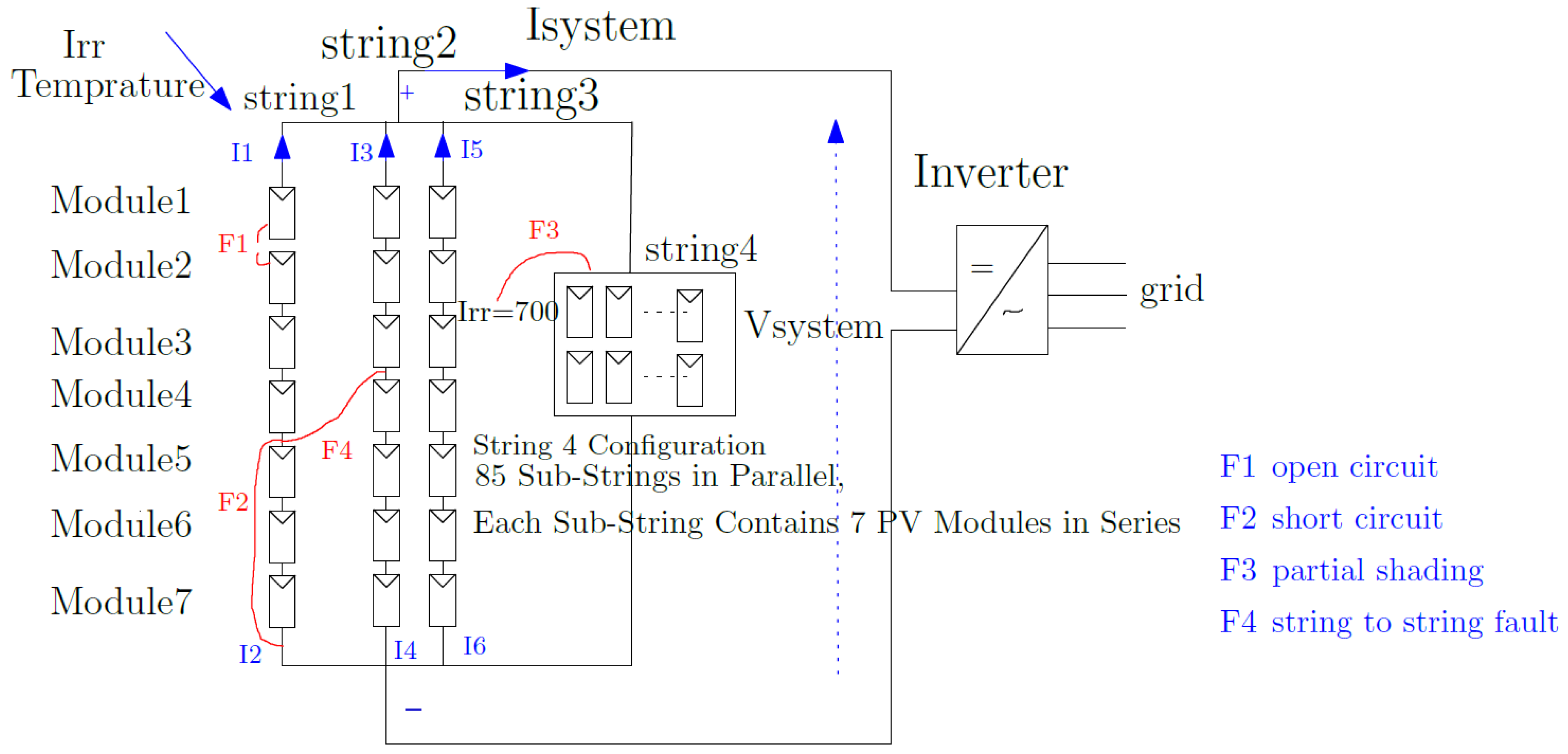
The simulated fault locations and their distributions across the PV array are illustrated in Figure 13.

As shown in Figure 13, the simulated faults were distributed across multiple strings within the PV array. The open-circuit and partial short-circuit faults were applied to String 1, the partial shading condition affected the 85-string array, and the string-to-string fault was introduced between Strings 1 and 2. This configuration ensures adequate spatial variation and realistic fault representation. Future work will further extend this setup to randomized fault placements for broader generalization.

Before presenting the detailed modeling and algorithmic procedures, the overall research workflow is outlined in Figure 14 to provide a clear overview of the study’s structure and methodological sequence.

5. Machine Learning-Based Fault Classification

This section presents the ML algorithms adopted for PV fault detection and classification. Three classifiers MLNN, SVM, and RF were implemented and trained using the same dataset derived from the simulated PV system. Each algorithm was selected based on its proven efficiency in handling nonlinear data, robustness against noise, and suitability for real-time diagnostic applications. The comparative analysis ensures a fair and consistent evaluation of model performance under identical operating and environmental conditions.

5.1. Multi-Layer Neural Network (MLNN)

5.1.1. MLNN Theoretical Background

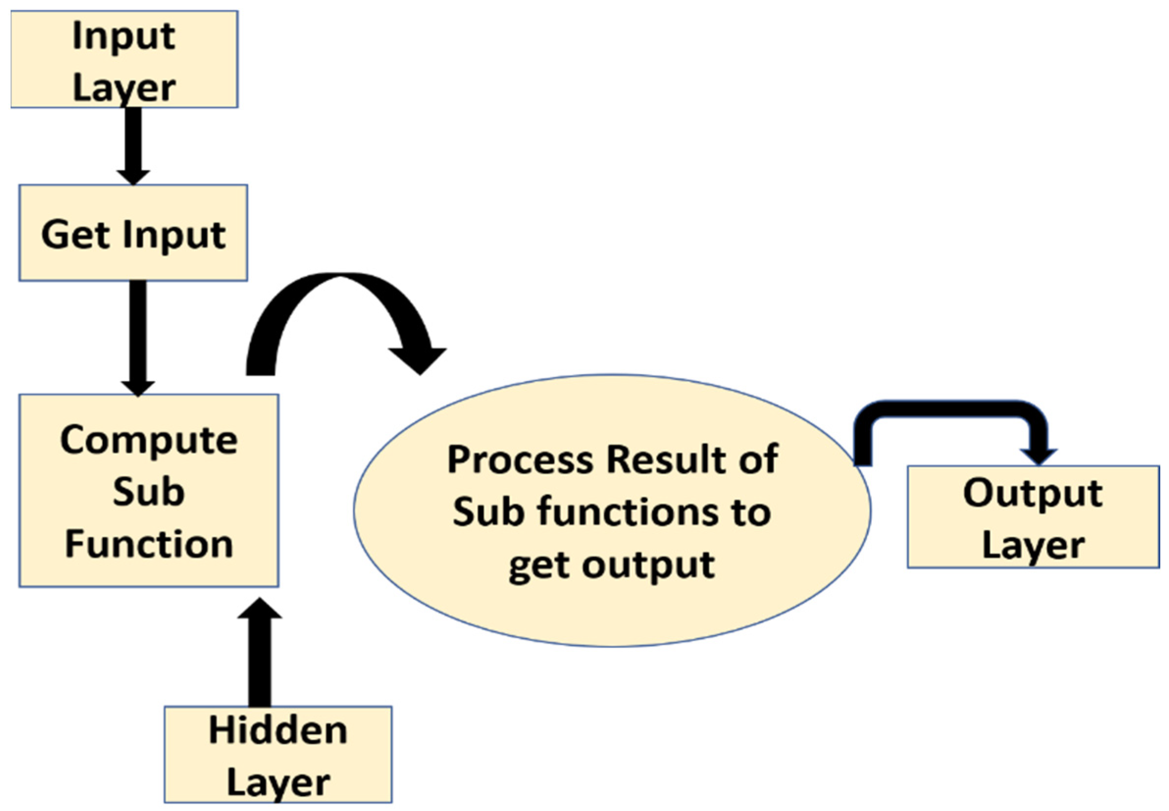
ANNs are computational models inspired by the architecture of biological neural systems. They consist of multiple interconnected processing units (“neurons”) organized in layers, and are capable of learning non-linear mappings using algorithms such as backpropagation. In PV fault diagnosis, ANNs have demonstrated high-dimensional data and can capture subtle patterns indicative of various fault conditions. Multi-class deep neural networks are used in the extraction process for non-linear classification issues. Multi-layer Perceptron fall within the category of nonlinear arrangements, meaning that complicated nonlinear data can be used in computing [24,25,26,27,28,29,30]. Every layer is connected to already-existing hidden units. The bias function assists each hidden unit in processing the weights. The organizing structure of MLNN is depicted in Figure 15, and the combined linear summation and activation function are produced as a single notation in multi-class classification problems.

As is well known, the Multilayer Perceptron (MLP) is a feed-forward ANN consisting of an input, one or more hidden, and an output layer. Each neuron, except those in the input layer, performs nonlinear approximation using an activation function such as Tanh, Sigmoid, or Rectified Linear Unit (ReLU), with ReLU often preferred for mitigating the vanishing gradient problem. The network is trained using the supervised back propagation algorithm [31,32,33].

5.1.2. Justification for MLNN Algorithm Selection

MLNN was chosen for its strong ability to model complex nonlinear relationships between current, voltage, irradiance, and temperature signals, which are inherently nonlinear in PV systems. In contrast to shallow learners such as SVM or RF, the MLNN can hierarchically extract high-level nonlinear features directly from raw signals, allowing more accurate classification of complex PV fault patterns. Its scalability and adaptive learning capability make it particularly suitable for large-scale PV datasets.

5.1.3. MLNN Implementation in This Study

The MLNN architecture designed for this work includes two hidden layers, each containing 30–50 neurons depending on data complexity and fault type and each employing the tansig activation function, followed by a softmax output layer for multi-class classification. The model was trained using the cross-entropy cost function and an adaptive learning rate strategy. The number of epochs was set to 300, with early stopping applied to prevent over fitting.

The inputs of a neuron are denoted as x₁, x₂, …, xₙ, with corresponding weights w₁, w₂, …, wᵢ. The output expression of a neuron is illustrated in Figure 16.

5.2. Support Vector Machine (SVM)

5.2.1. SVM Theoretical Background

SVM is a widely used supervised learning algorithm for classification and regression tasks, designed to identify the optimal hyperplane that separates classes in a high-dimensional feature space. By employing kernel functions such as linear, polynomial, radial basis function (RBF), sigmoid, or Gaussian, SVM can effectively handle both linear and non-linear data, making it suitable for a broad range of applications across various domains. In the case of regression problems, SVM is referred to as Support Vector Regression (SVR) [34]. The performance of the SVM model depends significantly on the choice of kernel function and its associated parameters including the scale parameter (γ), the regularization constant (C), and the error margin (ε). These parameters are typically optimized to achieve the best predictive accuracy.

The mathematical formulation of the SVM can be expressed as [24]

$$\mathrm{f}\left(\mathrm{x}\right)=\left(\mathsf{\omega },\mathsf{\phi }\left(\mathrm{x}\right)\right)+\mathrm{b}$$

(2)

where

• $\mathrm{f}\left(\mathrm{x}\right)$ represents the predicted output in a high-dimensional feature space;
• $\mathsf{\omega }$ is the weight vector associated with the output variable;
• $\mathsf{\phi }\left(\mathrm{x}\right)$ is the mapping function that transforms the input data into a higher-dimensional space;
• b is the bias term.

5.2.2. Justification for SVM Algorithm Selection

SVM was selected as a benchmark classifier because of its strong theoretical foundation and successful applications in electrical system diagnostics. It performs efficiently with small to medium-sized datasets and is effective in minimizing structural risk, leading to good generalization performance.

5.2.3. SVM Implementation in This Study

In this research SVM with a Radial Basis Function (RBF) kernel was implemented to capture nonlinear relationships among the PV parameters. The penalty parameter C and kernel coefficient γ were optimized empirically to achieve the best trade-off between bias and variance.

5.3. Random Forest (RF)

5.3.1. RF Theoretical Background

The RF algorithm, introduced is a robust ensemble learning technique widely applied to both classification and regression tasks [34]. It operates by constructing a large number of independent decision trees from randomly selected subsets of the training data and features. Each tree generates its own prediction, and the final output is obtained through a majority voting process for classification tasks or by averaging predictions for regression tasks. This approach significantly enhances predictive accuracy and reduces the risk of overfitting compared to using a single decision tree. The RF training process involves three key stages:

• Data Subdivision: The original dataset is randomly divided into multiple bootstrap samples.
• Tree Construction: Each tree is trained on its corresponding bootstrap sample using a random subset of features at each split, promoting diversity among the trees.
• Ensemble Aggregation: The predictions from all trees are aggregated through majority voting or averaging to produce the final result.

5.3.2. Justification for RF Algorithm Selection

Several advantages distinguish RF from other ML algorithms. These include its high classification accuracy, low generalization error, computational efficiency and relative ease of hyper parameter tuning during training. Furthermore, its ability to handle high-dimensional datasets, manage missing values, and capture complex, allowing it to effectively model complex dependencies across various application domains.

5.3.3. RF Implementation in This Study

In this study, the RF classifier was implemented using MATLAB’s Statistics and ML Toolbox. The model was trained and tested on the same dataset used for MLNN and SVM to ensure fair benchmarking. The optimal configuration was achieved by tuning key hyper parameters, including the number of trees, tree depth, and minimum leaf size.

The final model employed 100 decision trees, each with a maximum depth of 20, and used Gini impurity as the splitting criterion. These settings were determined empirically based on cross-validation to balance classification accuracy and computational efficiency as shown in

Table 3. Distribution of training and testing samples across the five operating classes.

Description	Train Count	Train %	Test Count	Test %	Class
Fault-free system	251	25.10%	37	18.5%	0
Open-circuit fault	167	16.70%	35	17.5%	1
Short-circuit fault	170	17.00%	42	21.00%	2
Partial shading	201	20.10%	47	23.00%	3
String to string fault	211	21.10%	39	19.5%	4
Total	1000	100%	200	100%	—

.

6. Methodology

This study employs a structured methodology for the development and evaluation of a fault classification and detection system for PV arrays using ML models. The process includes simulation-based data generation, feature extraction and preprocessing, model development, performance evaluation, and comparative analysis among three ML algorithms MLNN, SVM, and RF.

The methodology begins with simulating a 250 kW grid-connected PV system in MATLAB/Simulink, composed of 4 PV strings connected in parallel. Faults were systematically injected into the simulation to reflect five distinct operational scenarios: normal operation, open-circuit fault, partial short-circuit fault, partial shading, and string-to-string fault. Each fault scenario was applied at various string and module locations within the array to ensure diversity and enhance model generalization.

6.1. Data Generation and Labeling

For each scenario, data were generated by applying variable irradiance and temperature profiles to emulate real-world conditions. Faults were injected at different string and module positions to ensure data diversity and robustness.

During each simulation run, a set of raw electrical signals was recorded, including

• String currents (I₁ to I₆);
• Total current (Itotal);
• Station voltage (V_station);
• Total output power (P_total);
• Irradiance (Irr) and temperature (Tempr);
• Voltage of string 1 (V_string1).

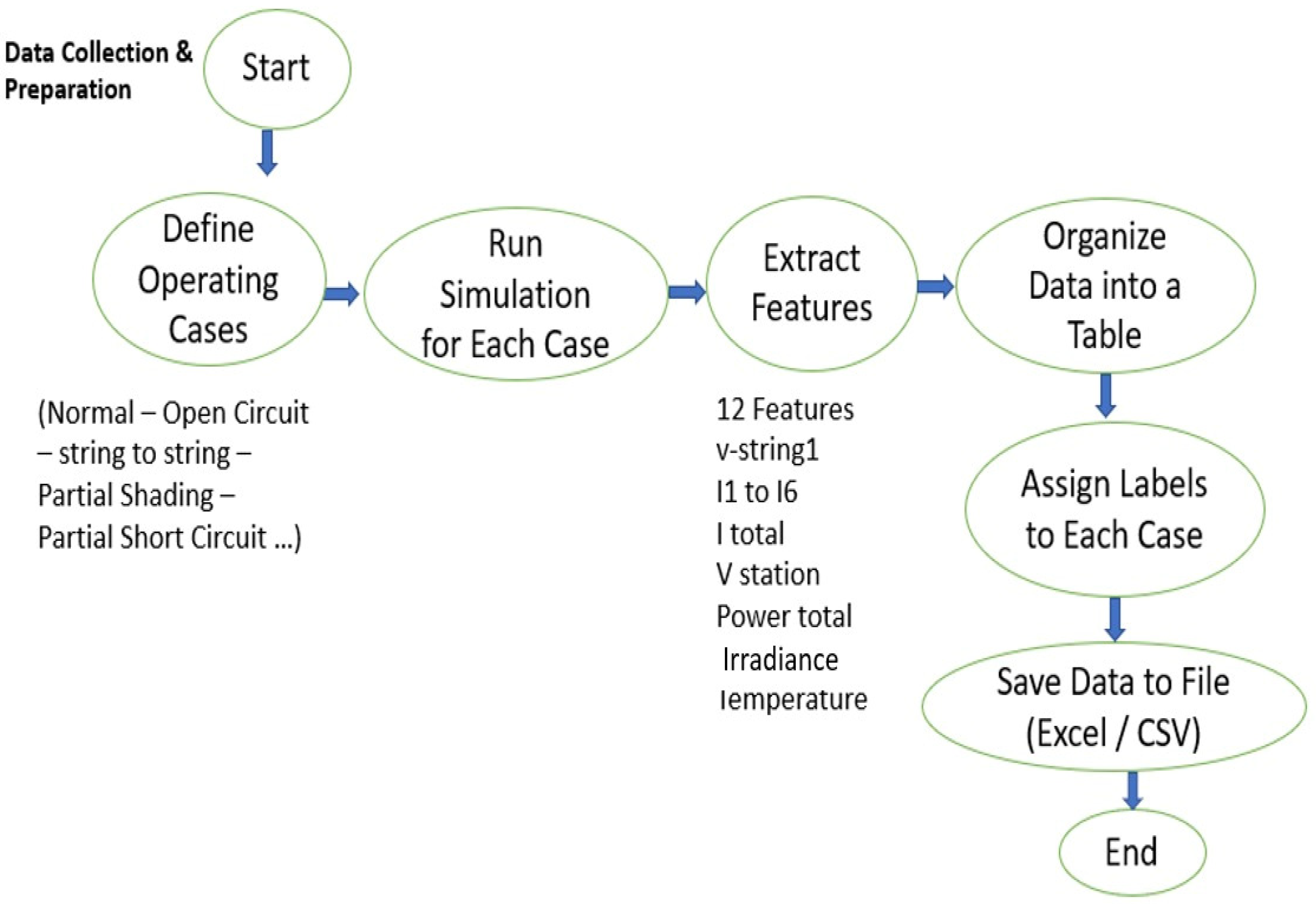
As shown in Figure 17 illustrates the data collection and preparation workflow. The process started by defining five operating scenarios The generated signals (voltage, current, total power, irradiance, and temperature) were then processed to extract 12 features, which were organized into labeled datasets. In total, 1000 samples were used for training and 200 samples for testing, as summarized in Table 3. The available dataset was divided into 1000 training samples and 200 testing samples, ensuring all five operating conditions were proportionally represented. During MLNN training, MATLAB automatically reserved approximately 15% of the training data for validation, used exclusively for monitoring network generalization and preventing overfitting. No manual data leakage occurred between the training, validation, and testing subsets.

6.2. Data Preprocessing and Model Training

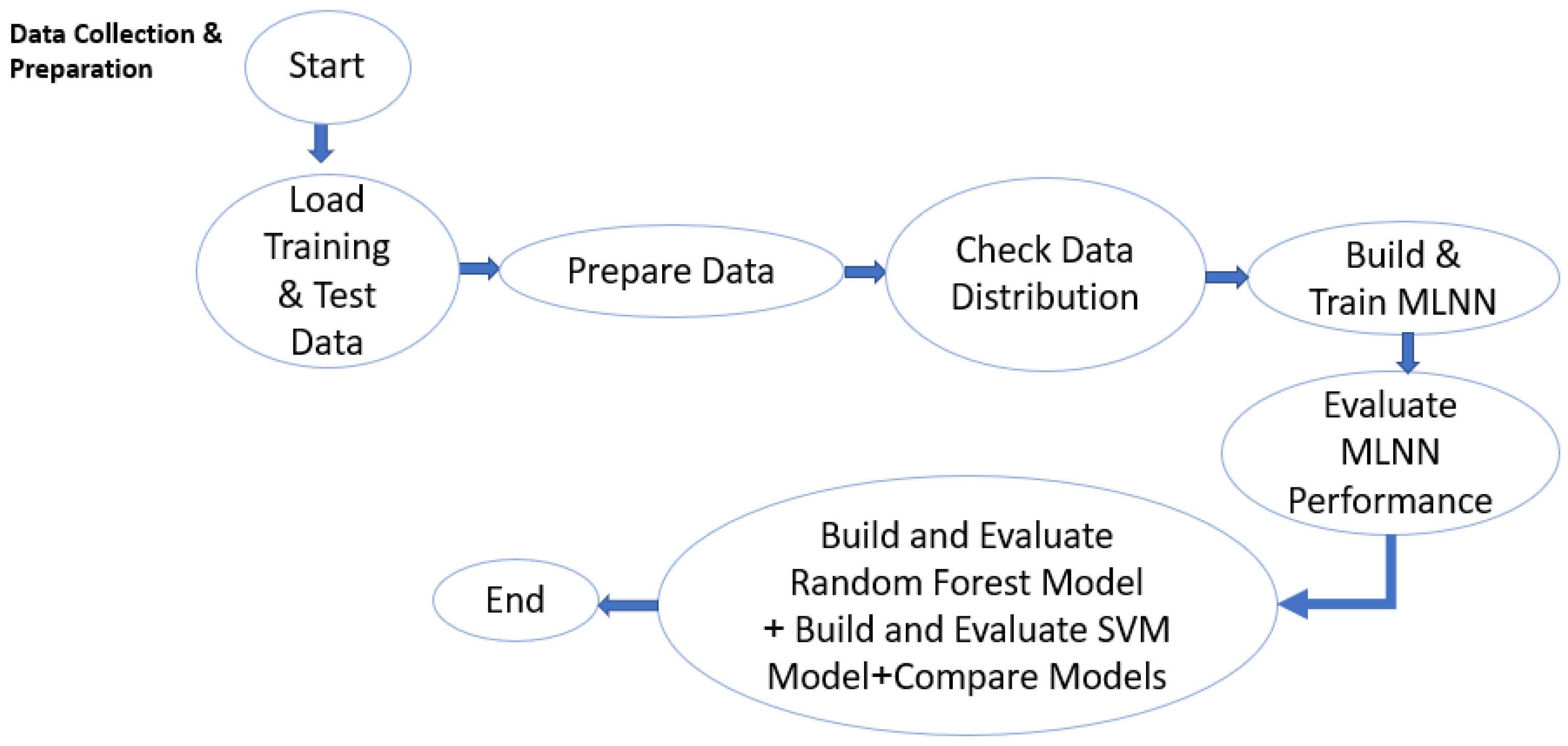
Before model training, the dataset was preprocessed to ensure consistency and comparability among all algorithms. In practical PV systems, measurement signals are often affected by different types of noise environmental, sensor, and electrical as summarized in

Table 4. Type of noise associated with PV panel.

Type of Noise	Description
Environmental	Changes in irradiance and temperature, shading from adjacent structures, and dust accumulation.
Sensor	Measurement errors, sensor drift, and EM interference.
Electrical	Power surges, grid voltage variations, and electrical interference from adjacent equipment.

. Identifying and reducing these noise sources is an essential preprocessing step to improve the reliability of the training data. The primary steps of the proposed method, including data preparation, model training, and performance comparison of the MLNN, RF, and SVM classifiers, are illustrated in the flowchart shown in Figure 18. All input features, including voltage, current, power, irradiance, and temperature, were normalized using z-score normalization to eliminate scale differences and accelerate model convergence. The class labels representing the five operating conditions were encoded using the one-hot encoding method, which prevents artificial ordinal relationships between categories and allows the MLNN model to process categorical targets effectively through its softmax output layer. In contrast, the SVM and RF models used integer class labels internally. This preprocessing step ensured fair comparison and stable performance across all models. The input features used for all three algorithms (MLNN, RF, and SVM) are summarized in

Table 5. Input features used for all three algorithms (MLNN, RF, and SVM).

No.	Symbol	Description
1	I1	The current is at the top of string 1
2	I2	The current is at the bottom of string 1
3	I3	The current is at the top of string 2
4	I4	The current is at the bottom of string 2
5	I5	The current is at the top of string 3
6	I6	The current is at the bottom of string 3
7	I-total	Total current of station
8	V-total	Total voltage of station
9	P-total	Total power of station
10	V-string1	Voltage of the first PV string
11	T	Ambient temperature (°C) (25–45 °C)
12	G	Solar irradiance (W/m2) (400–1000 W/m2)

.

6.2.1. MLNN Model

The MLNN consisted of an input layer, two hidden layers, and one output layer. The architecture of the MLNN is illustrated in Figure 19, showing the layered structure and neuron configuration.

The number of neurons in each layer was optimized empirically to achieve high accuracy while maintaining computational efficiency. The network structure and training parameters used for the MLNN model are summarized in

Table 6. Configuration and parameters of the MLNN model.

Parameters	Description
Input Variables	12 (I1–I6, V-total, P-total, I-total, V-string1, T, G)
Output variables	5 classes (Normal, Fault 1, Fault 2, Fault 3, Fault 4)
No. of Neurons	(30, 50) two hidden layers
No. of Layers	3 (input, 2 hidden, output)
Training Algorithm	Scaled Conjugate Gradient (trainscg)
Training process	Supervised learning with one-hot encoded targets
Activation function	tansig (hidden layers), softmax (output layer)
Learning Rate	Adaptive (auto optimized by SCG)
Epochs	300
Type of fault data samples	Non-linear PV fault data (normal & fault conditions)
Stopping Criteria	Early stopping based on validation performance
Data Preprocessing	Normalization + One-Hot Encoding
Performance Metrics	Accuracy, Precision, Recall, F1-score
Achieved Accuracy	98%

.

6.2.2. SVM Model

The SVM classifier utilized a linear kernel to separate the fault classes in the feature space. Since the data were already normalized and linearly separable to a reasonable extent, the linear kernel provided a good balance between accuracy and complexity. The structure and training parameters used for the SVM model are summarized in

Table 7. Configuration and parameters of the SVM model.

Parameters	Description
Input Variables	12 (I1–I6, V-total, P-total, I-total, V-string1, T, G)
Output variables	5 classes (Normal, Fault 1, Fault 2, Fault 3, Fault 4)
Model Type	SVM using fitcecoc for multi-class classification
Kernel Function	Linear (default kernel used by fitcecoc)
Coding Design	One-vs.-One (pairwise binary SVMs for multi-class classification)
Data Normalization	Yes (applied before training)
Training Process	Supervised classification
Performance Metrics	Accuracy, Precision, Recall, F1-score
Achieved Accuracy	80%

.

6.2.3. RF Model

The RF algorithm, based on ensemble learning, was implemented using 100 decision trees. Each tree was trained on a random subset of features and samples (bootstrap aggregation), and the final output was determined by majority voting among trees. The structure and training parameters used for the RF model are summarized in

Table 8. Configuration and parameters of the RF model.

Parameters	Description
Input Variables	12 (I1–I6, V-total, P-total, I-total, V-string1, T, G)
Output variables	5 classes (Normal, Fault 1, Fault 2, Fault 3, Fault 4)
Model Type	RF (Tree Bagger) MATLAB Ensemble Classifier
Number of Trees	100
Split Criterion	Gini impurity (default MATLAB setting)
Training process	Supervised learning with one-hot encoded targets
Maximum Depth	Automatic (determined by MATLAB)
Out-of-Bag Validation	Enabled (OOB Prediction, on)
Data Normalization	Yes (applied before training)
Training Process	Supervised classification
Performance Metrics	Accuracy, Precision, Recall, F1-score
Type of Fault Data	Non-linear PV fault data (normal and fault conditions)
Achieved Accuracy	91%

.

7. Results and Discussion

7.1. MLNN Training Performance

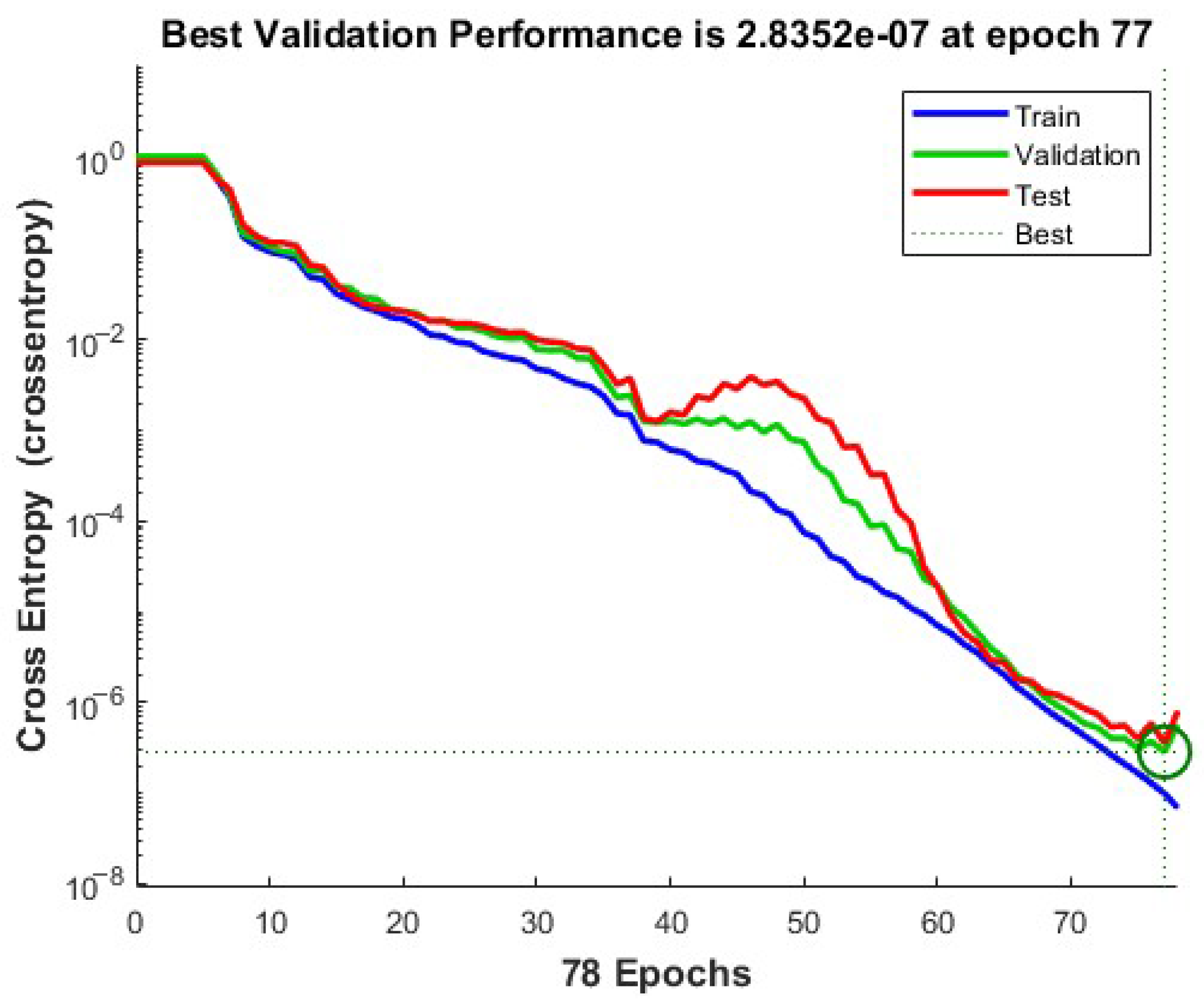
The Mean Squared Error (MSE) curve consistently decreased across the training, validation, and testing datasets, confirming the smooth convergence of the MLNN model and the absence of overfitting. As illustrated in Figure 20, the cross-entropy loss gradually declined for all datasets, with the best validation performance achieved at epoch 77. The close alignment between the training and validation curves further indicates stable learning behavior and reliable generalization capability.

As shown in Figure 20, MLNN training performance showing the cross-entropy loss convergence over 78 epochs. The training, validation, and testing curves decrease smoothly and align closely, indicating stable learning, no over fitting, and optimal validation performance achieved at epoch 77. Although the current dataset was noise-free, the robustness of the proposed MLNN model was indirectly evaluated through cross-validation and monitoring of validation loss, as shown in Figure 20. The close alignment between the training and validation curves indicates strong generalization and resistance to overfitting. In future work, sensor noise and measurement errors (e.g., ±1% Gaussian noise on voltage and current signals) will be simulated to further assess model robustness under real-world conditions.

7.2. Comparative Analysis with SVM and RF

For benchmarking purposes, two additional classification algorithms SVM and RF were implemented using the same dataset and preprocessing pipeline.

• The SVM model achieved a classification accuracy of 80%, indicating a moderate ability to distinguish between different PV fault classes.
• The RF model achieved a test accuracy of 91%, demonstrating strong classification performance and good generalization, although slightly lower than that of the MLNN.
• The MLNN model outperformed both, achieving a test accuracy of 98%, thereby demonstrating superior predictive accuracy and fault discrimination capability.

The superior performance of the MLNN can be attributed to its multilayer nonlinearstructure, which allows the network to learn intricate relationships between input features relationships that are often too complex for conventional classifiers like SVM and RF to capture effectively.

Collectively, these findings confirm that the proposed MLNN-based approach provides a reliable, scalable, and accurate solution for PV fault detection and classification, outperforming traditional ML techniques in both accuracy and stability

7.3. Confusion Matrix Analysis

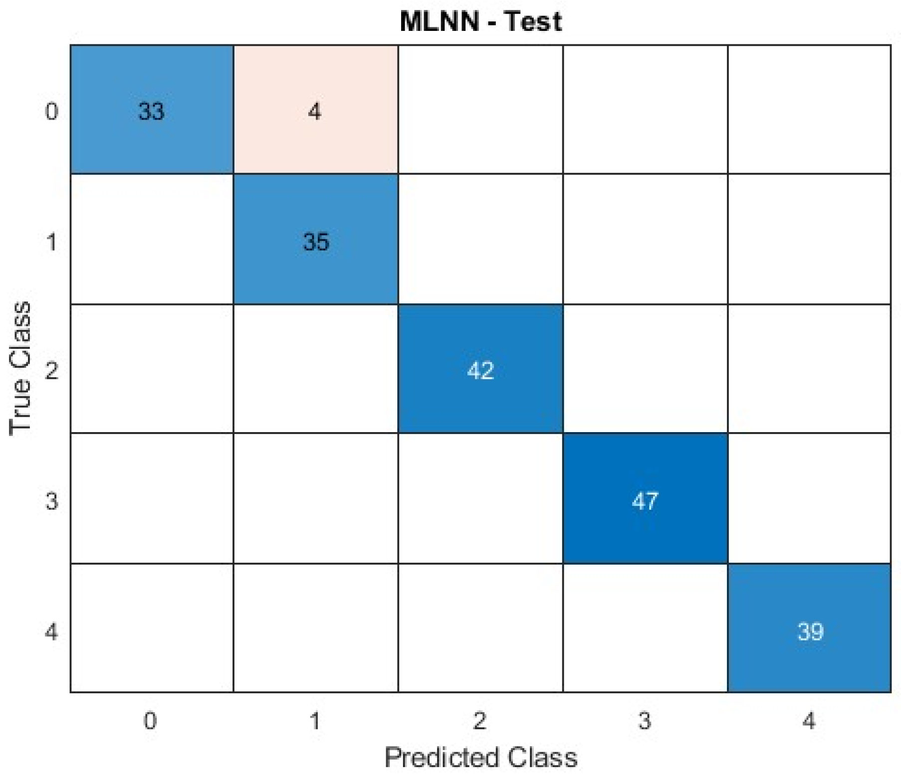
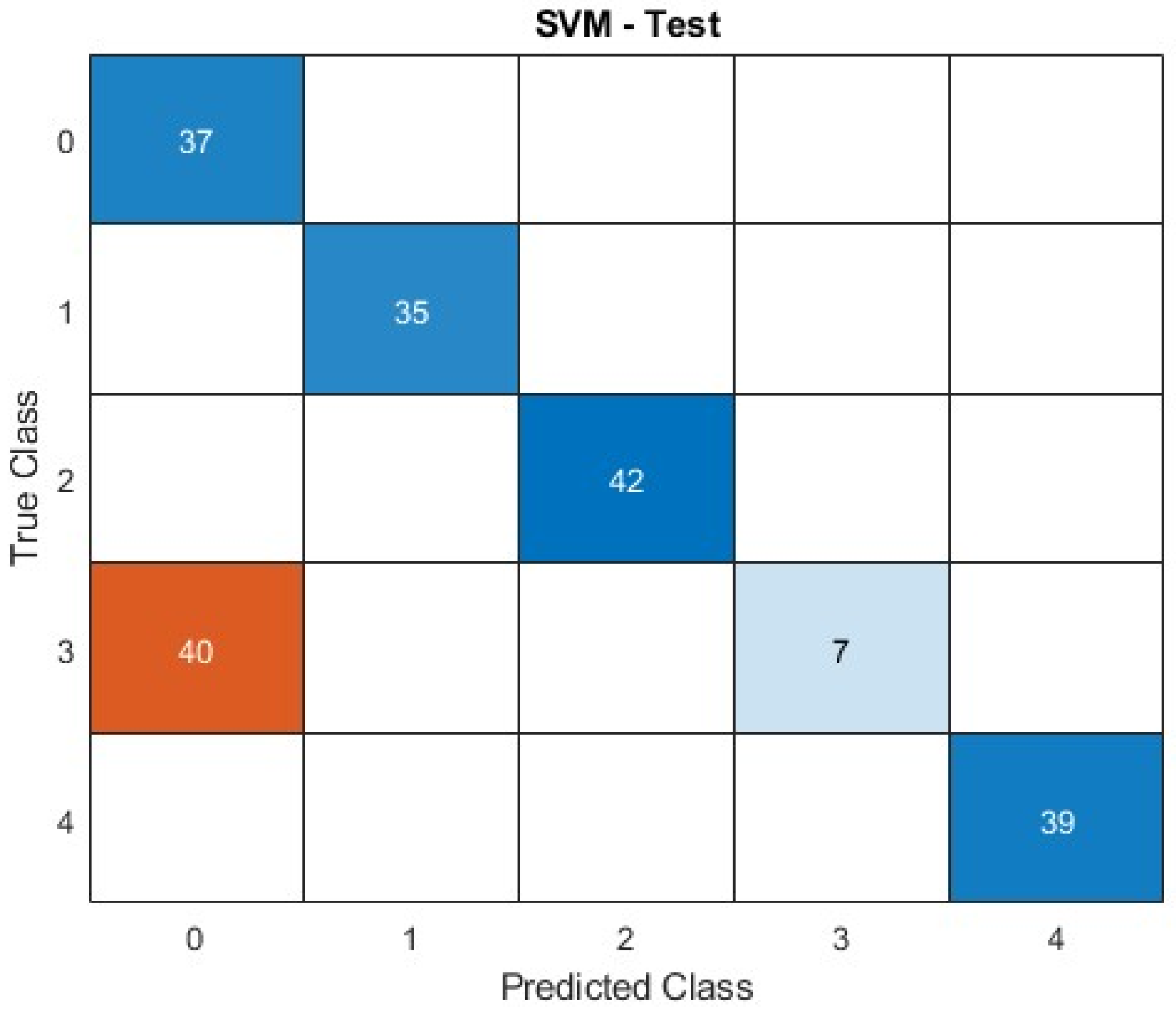
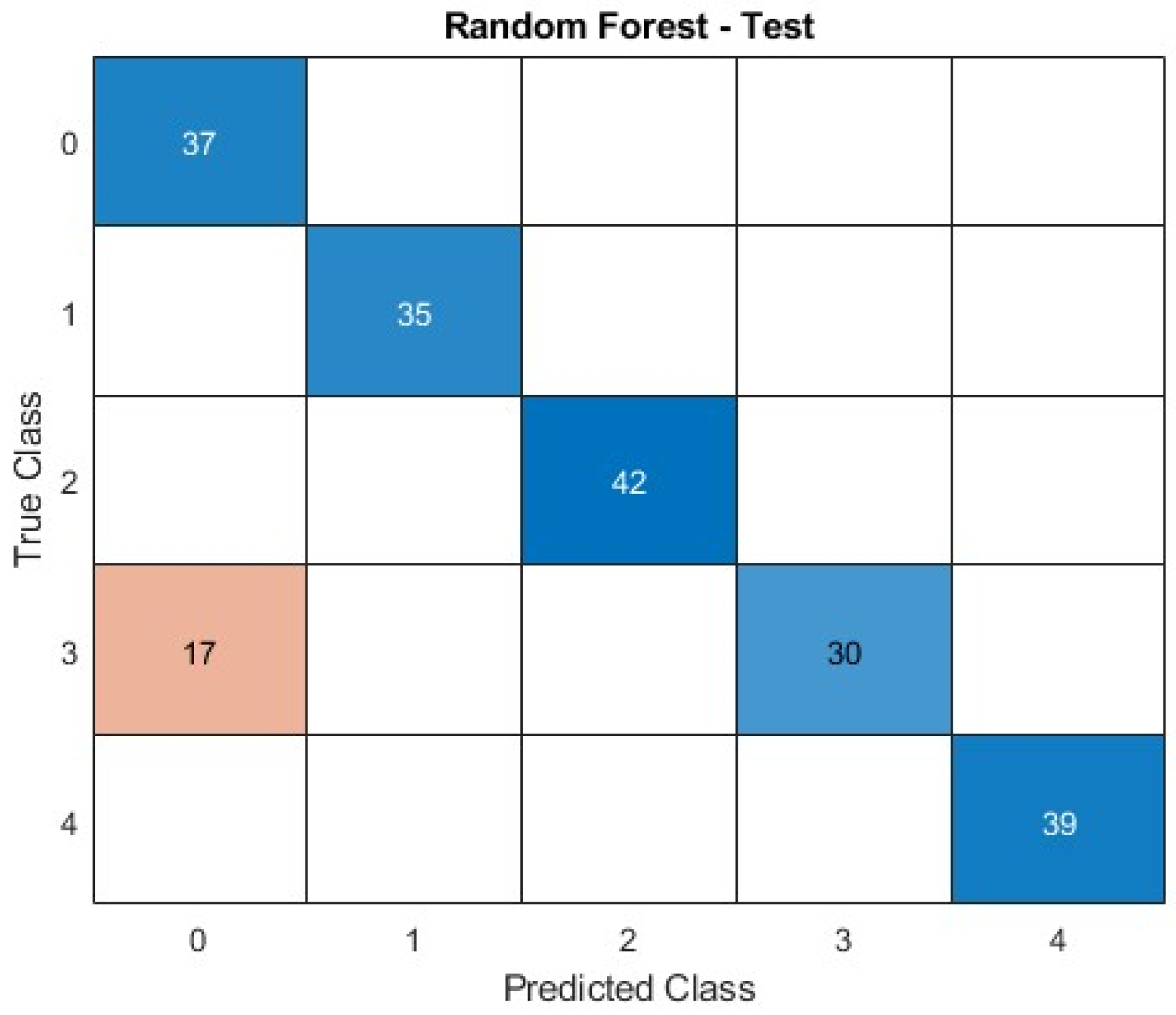
The confusion matrices for the PV fault diagnosis job show how the expected and actual classes relate to one another. The diagonal elements stand for correct classifications, and greater values denote better predicted ability. With only four samples from class 0 incorrectly identified as class 1, the MLNN classifier demonstrated its high discriminative capacity by achieving virtually flawless classification for the majority of classes. Despite incorrectly classifying 17 samples of class 3 as class 0, the RF model also demonstrated strong performance for classes 0, 1, 2, and 4. Class 3 had a significant decline in accuracy, with 40 samples wrongly classified as class 0 and only 7 correctly identified. In a similar vein, the SVM classifier maintained good accuracy for classes 0, 1, 2, and 4. These misclassifications, especially in class 3 (partial shading), occur because its electrical fingerprints overlap in feature space with those of partial short-circuit or string-to-string faults under specific irradiance and temperature conditions. However, the MLNN model exhibits good generalization across all fault types, and class 3’s overall accuracy is still satisfactory.

• Accuracy is calculated by dividing the total number of accurate predictions produced by the matrix by the total number of accurate predictions made of CI possible outputs [35,36,37,38,39]. The diagonal of the matrix values provides the possible outputs. Equation (3) provides the formulation of accuracy.

$$\mathrm{Accuracy} = {\displaystyle \frac{\sum _{\mathrm{i}=1}^{\mathrm{C}}{\mathrm{L}}_{\mathrm{i}\mathrm{i}}}{ \sum _{\mathrm{i}=1}^{\mathrm{C}}\mathrm{\ast }\sum _{\mathrm{j}=1}^{\mathrm{C}}{\mathrm{L}}_{\mathrm{i}\mathrm{j}}}}$$

(3)

• Precision the ratio of successfully predicted observations to the total number of observations that were correctly recognized is the formula that is used to compute precision, which is a measure of the positive predictive value. Precision is presented as a percentage.

$$\mathrm{precision}= {\displaystyle \frac{{\mathrm{L}}_{\mathrm{i}\mathrm{i}}}{\sum _{\mathrm{K}=1}^{\mathrm{n}}{\mathrm{L}}_{\mathrm{K}\mathrm{i}}}}$$

(4)

• Recall The sensitivity of a prediction model is defined as recall, and which is provided by the percentage of positive instances. The recall is supplied by the proportion of properly identified positive cases.

$$\mathrm{Recall}= {\displaystyle \frac{{\mathrm{L}}_{\mathrm{i}\mathrm{i}}}{\sum _{\mathrm{K}=1}^{\mathrm{n}}{\mathrm{L}}_{\mathrm{K}\mathrm{i}}}}$$

(5)

• F1 score is the arithmetic mean of the recall and accuracy scores.

$$\mathrm{F}1 \mathrm{s}\mathrm{c}\mathrm{o}\mathrm{r}\mathrm{e}={\displaystyle \frac{2 \mathrm{\ast } \mathrm{p}\mathrm{r}\mathrm{e}\mathrm{c}\mathrm{i}\mathrm{s}\mathrm{i}\mathrm{o}\mathrm{n} \mathrm{\ast } \mathrm{R}\mathrm{e}\mathrm{c}\mathrm{a}\mathrm{l}\mathrm{l}}{\mathrm{p}\mathrm{r}\mathrm{e}\mathrm{c}\mathrm{i}\mathrm{s}\mathrm{i}\mathrm{o}\mathrm{n}+\mathrm{R}\mathrm{e}\mathrm{c}\mathrm{a}\mathrm{l}\mathrm{l}}}$$

(6)

7.3.1. MLNN Confusion Matrix

Figure 21 illustrates the confusion matrix of the proposed MLNN model. The confusion matrix of the proposed MLNN model demonstrates an almost perfect classification performance across all fault categories. Only four samples belonging to class 0 were misclassified as class 1, while all other fault types were accurately identified. This indicates the network’s strong generalization capability and its high discriminative power in distinguishing between closely related PV fault conditions. The diagonal dominance of the matrix further confirms the robustness and reliability of the MLNN model in classifying multi-class PV faults.

7.3.2. SVM Confusion Matrix

As shown in Figure 22, the confusion matrix of the SVM classifier reveals a considerable level of misclassification, particularly for class 3 (partial shading), where 40 samples were incorrectly identified as class 0. In contrast, classes 0, 1, 2, and 4 were accurately classified with minimal errors. This outcome indicates the SVM’s limited capability to effectively separate overlapping feature patterns among certain PV fault types.

7.3.3. RF Confusion Matrix

As shown in Figure 23, the confusion matrix of the RF model demonstrates a reduced sensitivity to partial shading faults, as indicated by the notable misclassification between class 3 and class 0 where 17 samples were incorrectly categorized. Nevertheless, the model maintained reasonable prediction accuracy across most classes, confirming its generally strong yet slightly imbalanced classification performance.

7.4. Comparative Discussion

Comparison of the PV fault detection performance of MLNN, SVM, and RF classifiers is illustrated in

Table 9. Performance indices between MLNN, SVM and RF.

Performance Metric	Description	MLNN (%)	RF (%)	SVM (%)
Accuracy	Measures the proportion of correctly classified instances out of the total instances. A higher accuracy indicates better classification performance.	98%	91%	80%
Precision	Indicates the proportion of true positive predictions among all positive predictions. It measures the model’s ability to avoid false positives.	98%	93%	83%
Recall (Sensitivity)	Measures the proportion of true positive predictions among all actual positive instances. It evaluates the model’s ability to detect all positive instances.	98%	94%	90%
F1 Score	Harmonic means of precision and recall, provide a balance between the two metrics. It is useful when there is an uneven class distribution or misclassification costs.	98%	92%	78%

. The MLNN’s outstanding capacity to accurately identify and generalize fault types in PV systems is demonstrated by the performance metrics, which clearly reveal that it achieved the greatest accuracy, precision, recall, and F1 score (all at 98%). Because of its limited capacity to capture nonlinear relationships among the input data, SVM trailed behind RF, which achieved respectable performance with over 90% accuracy. These outcomes demonstrate that, across all evaluation metrics, the MLNN model offers a more dependable and consistent classification performance.

8. Conclusions

This study presented a fault classification and detection framework for PV systems based on ML techniques, utilizing a simulated 250 kW grid-connected PV model in MATLAB/Simulink. Five distinct operating conditions were simulated, including both normal and fault scenarios (open-circuit, partial short-circuit, partial shading, and string-to-string fault). Three classification models were evaluated: MLNN, SVM, and RF. Among the tested models, MLNN achieved the highest accuracy of 98%, demonstrating superior capability in learning non-linear relationships and extracting fault-specific features from noisy, raw signal data. RF followed with an accuracy of 91.5%, showing strong generalization performance across most fault classes. SVM achieved 80% accuracy, indicating moderate classification performance. These results underscore the critical importance of selecting classifiers that align with the nature of the input data and the operational complexity of PV systems. The findings confirm the effectiveness and robustness of MLNN models for real-time fault detection and classification in large-scale solar power plants, offering valuable potential for intelligent maintenance and enhanced system reliability

9. Future Work and Limitation of the Study

The results of this study confirm that the proposed MLNN-based framework effectively identifies and classifies various types of PV faults using simulated data. However, the main limitation of this work lies in its reliance on simulation-generated datasets, which may not fully capture the stochastic nature of real-world operating conditions such as sensor noise, degradation, and environmental fluctuations.

Building upon these promising results, several directions for future research are proposed.

First, advanced deep learning methodologies, including Convolutional Neural Networks (CNNs) and Long Short-Term Memory (LSTM) architectures, will be investigated to enhance feature extraction and temporal fault prediction accuracy.

Second, experimental validation will be conducted using real operational data from field-deployed PV systems to assess model robustness and generalization under realistic conditions.

Third, the integration of the proposed framework into IoT-based monitoring platforms will be explored to enable real-time fault detection and predictive maintenance. This step will transform the current simulation model into a practical, intelligent tool for autonomous PV system management.

Finally, the framework will be extended to address more complex fault scenarios, including grounding faults, bypass-diode failures, and arc faults. Additional simulation datasets will be generated to analyze their impacts on system performance and to further improve the diagnostic models’ generalization capability.

References

1. Abo-Alela, S.A.-Z. Design and performance of hybrid wind–solar energy generation system for efficiency improvement. J. Al-Azhar Univ. Eng. Sect. 2018, 13, 1118–1124. [Google Scholar] [CrossRef]
2. Mellit, A.; Tina, G.M.; Kalogirou, S.A. Fault detection and diagnosis methods for photovoltaic systems: A review. Renew. Sustain. Energy Rev. 2018, 91, 1–17. [Google Scholar] [CrossRef]
3. Patthi, S.; Arandhakar, S.; Reddy, L. Photovoltaic string fault optimization using multi-layer neural network technique. Results Eng. 2024, 22, 102299. [Google Scholar] [CrossRef]
4. Sera, D.; Teodorescu, R.; Rodriguez, P. PV panel model based on datasheet values. In Proceedings of the 2007 IEEE International Symposium on Industrial Electronics, Vigo, Spain, 4–7 June 2007; pp. 2392–2396. [Google Scholar] [CrossRef]
5. Ghoneim, S.S.; Rashed, A.E.; Elkalashy, N.I. Fault detection algorithms for achieving service continuity in photovoltaic farms. Intell. Autom. Soft Comput. 2021, 29, 467–479. [Google Scholar] [CrossRef]
6. Mellit, A.; Kalogirou, S.A. Assessment of machine learning and ensemble methods for fault diagnosis of photovoltaic systems. Renew. Energy 2022, 184, 1074–1090. [Google Scholar] [CrossRef]
7. Li, B.; Delpha, C.; Diallo, D.; Migan-Dubois, A. Application of artificial neural networks to photovoltaic fault detection and diagnosis: A review. Renew. Sustain. Energy Rev. 2021, 138, 110512. [Google Scholar] [CrossRef]
8. Abubakar, A.; Almeida, C.F.M.; Gemignani, M. Review of artificial intelligence-based failure detection and diagnosis methods for solar photovoltaic systems. Machines 2021, 9, 328. [Google Scholar] [CrossRef]
9. Sepúlveda-Oviedo, E.H.; Travé-Massuyès, L.; Subias, A.; Pavlov, M.; Alonso, C. Fault diagnosis of photovoltaic systems using artificial intelligence: A bibliometric approach. Heliyon 2023, 9, e21491. [Google Scholar] [CrossRef]
10. Pratama, G.S.A.; Suharyanto, H.E.H.; Arif, Y.C. Identify and locating the faults in the photovoltaic array using neural network. J. Nas. Tek. Elektro 2021, 10. [Google Scholar] [CrossRef]
11. Chine, W.; Mellit, A.; Lughi, V.; Malek, A.; Sulligoi, G.; Pavan, A.M. A novel fault diagnosis technique for photovoltaic systems based on artificial neural networks. Renew. Energy 2016, 90, 501–512. [Google Scholar] [CrossRef]
12. Liu, Y.; Wu, Y. Fault diagnosis of photovoltaic modules: A review. Sol. Energy 2025, 293, 113489. [Google Scholar] [CrossRef]
13. Eldeghady, G.S.; Kamal, H.A.; Hassan, M.A.M. Comparative analysis of the performance of supervised learning algorithms for photovoltaic system fault diagnosis. Sci. Technol. Energy Transit. 2024, 79, 27. [Google Scholar] [CrossRef]
14. Thakfan, A.; Bin Salamah, Y. Artificial-intelligence-based detection of defects and faults in photovoltaic systems: A survey. Energies 2024, 17, 4807. [Google Scholar] [CrossRef]
15. Kumar, P.; Kumar, M.; Bansal, A.K. Monitoring of grid-connected photovoltaic systems using multilayer neural networks. In Proceedings of the 2023 9th International Conference on Signal Processing and Communication (ICSC), Noida, India, 21–23 December 2023; pp. 380–386. [Google Scholar] [CrossRef]
16. Breiman, L. Random forests. Mach. Learn. 2001, 45, 5–32. [Google Scholar] [CrossRef]
17. Amiri, A.F.; Oudira, H.; Chouder, A.; Kichou, S. Faults detection and diagnosis of PV systems based on machine learning approach using random forest classifier. Energy Convers. Manag. 2024, 301, 118076. [Google Scholar] [CrossRef]
18. Wang, K.; Zhong, Y.; Luo, X. Photovoltaic array fault detection based on manifold learning and neural network. In Proceedings of the 2024 5th International Conference on Computer Vision, Image and Deep Learning (CVIDL), Zhuhai, China, 19–21 April 2024; pp. 1104–1109. [Google Scholar] [CrossRef]
19. Ahmed, M.K. On-grid photovoltaic system maximum power point tracking using perturb and observe algorithm. J. Al-Azhar Univ. Eng. Sect. 2019, 14, 1113–1122. [Google Scholar] [CrossRef]
20. Hussain, I.; Agarwal, R.K.; Singh, B. MLP control algorithm for adaptable dual-mode single-stage solar PV system tied to three-phase voltage-weak distribution grid. IEEE Trans. Ind. Inform. 2018, 14, 2530–2538. [Google Scholar] [CrossRef]
21. AbdulMawjood, K.; Refaat, S.S.; Morsi, W.G. Detection and prediction of faults in photovoltaic arrays: A review. In Proceedings of the 2018 IEEE 12th International Conference on Compatibility, Power Electronics and Power Engineering (CPE-POWERENG 2018), Doha, Qatar, 10–12 April 2018. [Google Scholar] [CrossRef]
22. Betti, A.; Tucci, M.; Crisostomi, E.; Piazzi, A.; Barmada, S.; Thomopulos, D. Fault prediction and early detection in large PV power plants based on self-organizing maps. Sensors 2021, 21, 1687. [Google Scholar] [CrossRef]
23. Dhimish, M. Fault Detection and Performance Analysis of Photovoltaic Installations. Ph.D. Thesis, University of Huddersfield, Huddersfield, UK, 2018. [Google Scholar] [CrossRef]
24. Oruc, S.; Hinis, M.A.; Tugrul, T. Evaluating performances of LSTM, SVM, GPR, and RF for drought prediction in Norway: A wavelet decomposition approach on regional forecasting. Water 2024, 16, 3465. [Google Scholar] [CrossRef]
25. Li, J.; Chang, J.; Zhang, Y. Gradient descent optimization-based SINS self-alignment method and error analysis. IEEE Access 2021, 9, 8286–8298. [Google Scholar] [CrossRef]
26. Gaber, M.; Hamad, M.S.; El-Banna, S.H.; El-Dabah, M. An intelligent energy management system for ship hybrid power system based on renewable energy resources. J. Al-Azhar Univ. Eng. Sect. 2021, 16, 712–723. [Google Scholar] [CrossRef]
27. Eskandari, A.; Milimonfared, J.; Aghaei, M. Fault detection and classification for photovoltaic systems based on hierarchical classification and machine learning technique. IEEE Trans. Ind. Electron. 2020, 68, 12750–12759. [Google Scholar] [CrossRef]
28. Worku, M.Y.; Hassan, M.A.; Maraaba, L.S.; Shafiullah, M.; Elkadeem, M.R.; Hossain, M.I.; Abido, M.A. A comprehensive review of recent maximum power point tracking techniques for photovoltaic systems under partial shading. Sustainability 2023, 15, 11132. [Google Scholar] [CrossRef]
29. Petrone, G.; Spagnuolo, G.; Vitelli, M. A multivariable perturb-and-observe maximum power point tracking technique applied to a single-stage photovoltaic inverter. IEEE Trans. Ind. Electron. 2010, 58, 76–84. [Google Scholar] [CrossRef]
30. Gharib, Y.; Anis, W.; AbdelRahim, M. Enhancement maximum power point tracking of PV systems using different algorithms. J. Al-Azhar Univ. Eng. Sect. 2018, 13, 1290–1299. [Google Scholar] [CrossRef]
31. Liu, Y.; Chen, X.; Xu, L.; Li, H.; Li, M. A resource-aware parallelized backpropagation neural network in enabling efficient large-scale digital health data processing. IEEE Access 2019, 7, 114700–114713. [Google Scholar] [CrossRef]
32. Zhao, Y.; De Palma, J.F.; Mosesian, J.; Lyons, R.; Lehman, B. Line–line fault analysis and protection challenges in solar photovoltaic arrays. IEEE Trans. Ind. Electron. 2012, 60, 3784–3795. [Google Scholar] [CrossRef]
33. Akhtar, Z.; Naqvi, S.Z.A.; Hamayun, M.T.; Ijaz, S. A multilayer neural-network-based fault estimation and fault-tolerant control scheme for uncertain systems. Int. J. Robust Nonlinear Control 2024, 34, 11985–12011. [Google Scholar] [CrossRef]
34. Et-Taleby, A.; Chaibi, Y.; Benslimane, M.; Boussetta, M. Applications of machine learning algorithms for photovoltaic fault detection: A review. Stat. Optim. Inf. Comput. 2023, 11, 168–177. [Google Scholar] [CrossRef]
35. Garud, K.S.; Jayaraj, S.; Lee, M.Y. A review on modeling of solar photovoltaic systems using artificial neural networks, fuzzy logic, genetic algorithm and hybrid models. Int. J. Energy Res. 2021, 45, 6–35. [Google Scholar] [CrossRef]
36. Elnagi, M.; Kamel, S.; Ramadan, A.; Elnaggar, M.F. Photovoltaic models parameters estimation based on weighted mean of vectors. Comput. Mater. Contin. 2023, 74, 5229. [Google Scholar] [CrossRef]
37. Haseeb, M.; Mansour, A.H.I.; Othman, E.-S.A. Enhancing of single-stage grid-connected photovoltaic system using fuzzy logic controller. Int. J. Electr. Comput. Eng. 2024, 14, 2400–2412. [Google Scholar] [CrossRef]
38. Ali, M.H.; Zakaria, M.; El-Tawab, S. A comprehensive study of recent maximum power point tracking techniques for photovoltaic systems. Sci. Rep. 2025, 15, 14269. [Google Scholar] [CrossRef] [PubMed]
39. Torad, M.M.; Diab, A.A.Z.; Elbanna, S.H.A.; El-Dabah, M.A. Optimum sizing of hybrid renewable energy system with biomass backup of Egypt’s Western Desert. Ain Shams Eng. J. 2025, 16, 103402. [Google Scholar] [CrossRef]
Figure 1. Equivalent circuit for one-diode model.
Processes 13 03831 g001
Figure 2. Block diagram of the PV fault monitoring and classification system: (a) PV system section and (b) data-driven fault detection framework.
Processes 13 03831 g002
Figure 3. Classification of faults in PV array.
Processes 13 03831 g003
Figure 4. Configuration of the PV system under normal condition.
Processes 13 03831 g004
Figure 5. (a) Total current, (b) total voltage, and (c) total power at the DC side of the PV system under normal operating conditions.
Processes 13 03831 g005
Figure 6. PV system configuration under open-circuit fault in String 1.
Processes 13 03831 g006
Figure 7. (a) Total current, (b) total voltage, and (c) total power at the DC side of the PV system under open circuit fault conditions at the DC side.
Processes 13 03831 g007
Figure 8. PV system configuration under partial short-circuit fault.
Processes 13 03831 g008
Figure 9. (a) Total current, (b) total voltage, and (c) total power at the DC side of the PV system under partial short-circuit fault at the DC side.
Processes 13 03831 g009
Figure 10. (a) Total current, (b) total voltage, and (c) total power at the DC side of the PV system under partial shading at the DC side.
Processes 13 03831 g010
Figure 11. String-to-string fault between string 1 and string 2.
Processes 13 03831 g011
Figure 12. (a) Total current, (b) total voltage, and (c) total power at the DC side of the PV system under string-to-string fault at the DC side.
Processes 13 03831 g012
Figure 13. Simulated fault locations and their distribution across the PV array.
Processes 13 03831 g013
Figure 14. Flowchart of the proposed PV fault detection methodology.
Processes 13 03831 g014
Figure 15. Step-by-step layout of MLNN.
Processes 13 03831 g015
Figure 16. Diagram for mathematical equation of MLNN.
Processes 13 03831 g016
Figure 17. Workflow of data collection.
Processes 13 03831 g017
Figure 18. Workflow of the proposed fault detection process.
Processes 13 03831 g018
Figure 19. MLNN architecture for PV fault classification.
Processes 13 03831 g019
Figure 20. MLNN training loss (cross-entropy).
Processes 13 03831 g020
Figure 21. The confusion matrix of the MLNN model.
Processes 13 03831 g021
Figure 22. The confusion matrix of the SVM model.
Processes 13 03831 g022
Figure 23. The confusion matrix of the RF model.
Processes 13 03831 g023