Analysis of Flow Characteristics and Structural Optimization of High-Strength Cooling Equipment for Hot-Rolled Strip Steel

Abstract

High-strength cooling collectors are the key equipment for post-roll cooling technology of hot-rolled plates, and the internal flow characteristics of the collector are crucial to the quality and efficiency of cooling. In this work, numerical simulation is used to study the collector w₂ (collector width), β (manifold inclination), and h₂ (slot height) in different process parameters at the outlet of the velocity size and uniformity of the influence of the law. By comparing the two methods of steady state and transient state, the average velocity and flux errors are less than 0.1, and the effects of structural modifications on the outlet flow velocity and flow field uniformity were obtained for two sizes of trough nozzles. The results show that the increase in pressure increases the fluctuation in velocity, but the increase in velocity in the center of the slot outlet keeps decreasing; when the height of the tank h₁ = 90 mm, the increase in β causes the velocity of the slot outlet to decrease, but the fluctuation in velocity increases; when h₂ increases, the fluctuation in the velocity in the center of the slit outlet is obviously reduced, and the fluctuation is reduced most significantly when it is increased to 9 mm, but it will result in the decrease in the average value of the outlet velocity. Therefore, within the scope of this study, the optimal process parameters are inlet pressure 0.5–0.6 MPa, β = 10°, h₂ = 9–15 mm, and w₂ = 100–110 mm.

1. Introduction

Recent years have seen significant innovation, with innovative jet impingement-based cooling systems delivering impressive performance while maintaining affordability and high-performance hot-rolled steel production. As a key component of the high-strength cooling collector tube, the slit nozzle significantly impacts factors such as the velocity and uniformity of the jet at the outlet, which in turn influences cooling efficiency. During the cooling of hot-rolled steel strips, these factors play a critical role in determining the overall performance of the process, that is, the cooling medium delivered under a certain pressure or at a certain speed through the outlet jet to the processing surface. Due to the direct contact between the cooling medium and the machining surface, the flow boundary layer on the impacted surface is thin, making the impacted area produce a strong heat transfer effect, which is a highly efficient cooling method [1].

Numerical simulation offers several advantages over experimental methods, not only in terms of faster computation, but also in terms of cost reduction. By employing the finite element method, the computational fluid dynamics (CFD) software (ANSYS Fluent 2022 R2) enables a systematic study of the flow patterns and thermal performance of cooling devices [2,3]. Lytle et al. [4] investigated air jet impingement heat transfer at different spray spacing. Katti et al. [5] carried out experimental and theoretical analysis of local heat transfer by air jet impingement on a smooth plane using a circular straight tube nozzle. Nirmalkumar et al. [6,7,8,9] carried out extensive studies to analyze the slit jet impingement hydrodynamic properties and heat transfer distributions for different scenarios. In a follow-up study, Wang et al. [10,11,12] numerically simulated the behavior of a semi-closed slot jet using different turbulence models. From the analysis, it was determined that the RNG k-ε turbulence model delivers superior predictive performance compared to other models. Yan et al. [13] conducted a study on the drag-reduction behavior of cylindrical swirling flows with various asymmetric notch configurations using numerical simulation and particle image velocimetry. It was shown that different recesses have a positive effect on flow characteristics, but the improvement effect diminishes with the increase in the number of recesses. Azimi [14] investigated the heat transfer characteristics of a channel air jet impinging on a thermostatic concave surface under annular conditions. Meanwhile, Guoyong et al. [15,16] conducted a study on the flow behavior and thermal performance of jet flows from channel nozzles operating in high-pressure zones. Their research identified the optimal ranges for parameters such as the installation angle, the spacing between the nozzle and the steel plate, and the width of the jet slot. The results indicated that a slot width of approximately 2 mm offers the most cost-effective and efficient performance for high-pressure quenching processes.

Garimeela et al. [17,18,19,20] simulated the application of Reynolds number, Prandtl number, nozzle to plate spacing, nozzle spacing, as well as nozzle angle in different fields and its effect on heat transfer performance. Soyama et al. [21,22] did extensive research and analysis on the effect of nozzle geometry on the heat transfer generated by impingement jets. Wu Zebing et al. [23,24] simulated the cavitation strength of cross, Y, flat, and two-stage nozzles, and derived the corresponding cavitation jet characteristics. Li et al. [25] compared the heat transfer performance of straight cone nozzles and angular nozzles, and concluded that the angular nozzles have better heat transfer performance and cooling uniformity.

In summary, the majority of existing studies have predominantly focused on the investigation of flow dynamics and heat transfer mechanisms governing the interaction between impinging jets and cooling surfaces, with most analyses conducted based on two-dimensional numerical models. Nevertheless, research concerning the internal flow behavior within three-dimensional configurations of complex structures that incorporate fundamental geometric parameters remains relatively limited. Accordingly, the present study aims to elucidate the flow characteristics within a three-dimensional high-strength cooling manifold and to evaluate the influence of key structural parameters on jet velocity distribution and flow uniformity at the outlet. Unlike the previous work, this study examines fully three-dimensional configurations, providing a more accurate representation of real-world cooling systems, and explores the effects of these parameters in the context of high-performance steel production. These findings offer novel insights for optimizing cooling system designs to enhance heat transfer efficiency and uniformity.

2. Modeling and Methodology

2.1. Modeling

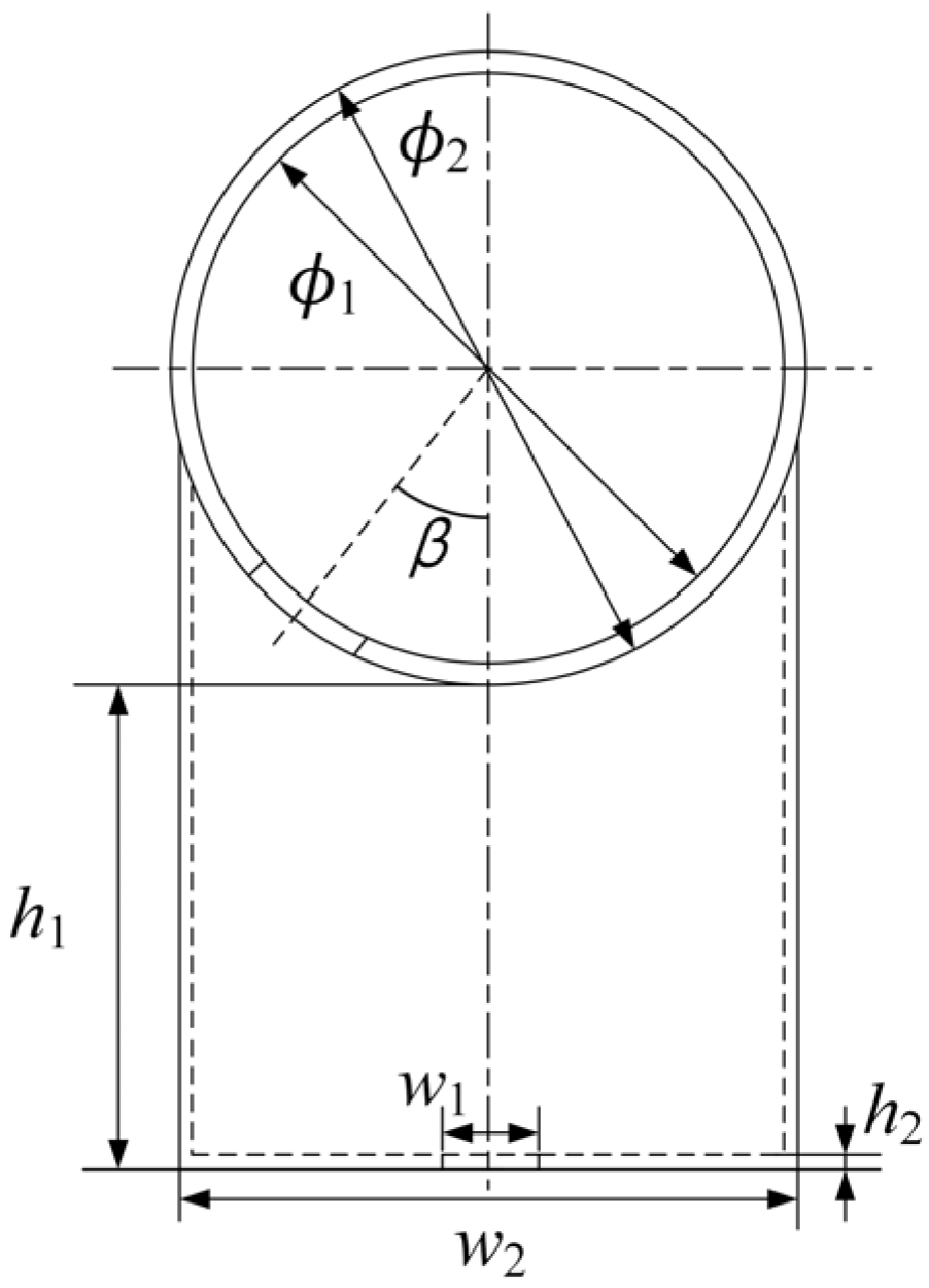
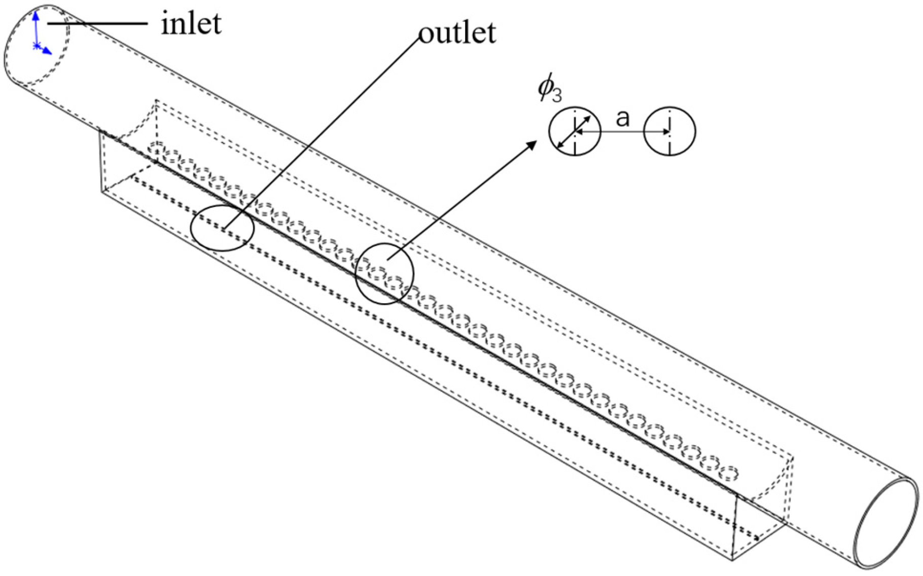
The focus of this study is a high-efficiency cooling header designed for reducing the temperature of hot-rolled steel during high-temperature processing. When the slot length is 1500 mm, the length of the main pipe L = 2000 mm, and the horizontal distance between the slot and the main pipe inlet and the rightmost wall is 250 mm; when the slot length is 2160 mm, the length of the main pipe L = 2160 mm, and the horizontal distance between the slot and the main pipe inlet and the rightmost wall is 200 mm. The initial model was characterized by the following key dimensions: an inner diameter of 150 mm for the main pipe (ϕ₁), an outer diameter of 160 mm (ϕ₂), and a diversion hole diameter of 30 mm (ϕ₃); the spacing between diversion holes (a) was 40 mm, and the height of the tank (h₁) was 90 mm. The header’s performance was evaluated by analyzing the influence of variations in slit and nozzle geometry on jet outlet velocity. The velocity fluctuations and their corresponding flux were continuously recorded. When the outlet slot width (w₁) was fixed at 2 millimeters, a detailed investigation was conducted to evaluate the effects of systematically varying the buffer platform height (h₃); the investigation also evaluated the effects of modifying the chamfer height (h₄). The influence of angle (α) as a significant factor must also be evaluated. Details of the model configuration are illustrated in Figure 1 and Figure 2.

2.2. Research Methods

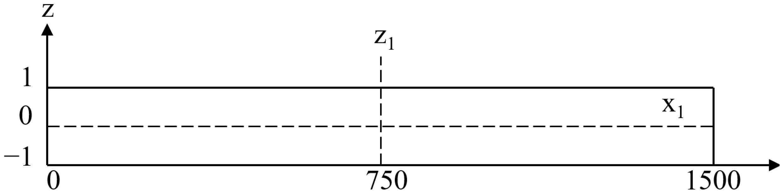
The computations were performed using a three-dimensional model. Therefore, the plane setting method is a commonly employed approach for boundary conditions. At the entrance of the main water supply pipe, a pressure boundary condition was imposed, and the inlet pressure was defined as 0.5 MPa, ensuring a uniform pressure distribution at the inlet boundary. Along the slot outlet, the centerlines x₁ and z₁ were introduced in the lengthwise and widthwise directions, respectively, as shown in Figure 3.

The inlet pressure is defined relative to atmospheric pressure (gauge pressure), which corresponds to actual industrial operating conditions where the cooling system is pressurized with respect to the ambient environment. Using gauge pressure therefore ensures consistency with engineering practice and with the real operating parameters of water-cooling systems. This study aims to evaluate how structural parameters affect outlet velocity and flow uniformity under a controlled supply pressure, and defining the inlet as a pressure boundary condition ensures meaningful comparison across different geometries.

The analysis was carried out in a sequential manner. First, the velocity distribution at the slot outlet was examined to understand the spatial variation in flow along the centerlines. Next, the average velocity across the outlet plane was calculated to provide a representative measure of the overall flow rate. Finally, additional parameters such as the velocity difference—defined as the difference between the maximum and minimum velocities—were evaluated to quantify the non-uniformity of the flow.

These analyses allowed for a comprehensive assessment of the flow characteristics and provided the basis for subsequent comparisons between different operating conditions. The calculations were performed using a steady-state, one-way flow model. Turbulence was modeled using the standard k–ε model, and the nonlinear equations were solved using the SIMPLE algorithm. For all remaining boundaries, wall-type boundary conditions were imposed. The working fluid is water, with a density of 996 kg·m⁻³ and kinematic viscosity of 8.6 ×10⁻⁷ m²/s.

2.3. Control Equation

The mass conservation in the fluid domain is described by the continuity equation, which can be written as follows:

$${\displaystyle \frac{\mathsf{\partial }u}{\mathsf{\partial }x}}+{\displaystyle \frac{\mathsf{\partial }v}{\mathsf{\partial }y}}+{\displaystyle \frac{\mathsf{\partial }w}{\mathsf{\partial }z}}=0$$

(1)

The momentum conservation equation is as follows:

$${\displaystyle \frac{\mathsf{\partial }u}{\mathsf{\partial }t}}+u{\displaystyle \frac{\mathsf{\partial }u}{\mathsf{\partial }x}}+v{\displaystyle \frac{\mathsf{\partial }u}{\mathsf{\partial }y}}+w{\displaystyle \frac{\mathsf{\partial }u}{\mathsf{\partial }z}}=f_x-{\displaystyle \frac{1}{\rho }}{\displaystyle \frac{\mathsf{\partial }p}{\mathsf{\partial }x}}+{\displaystyle \frac{\mu }{\rho }}\left({\displaystyle \frac{{\mathsf{\partial }}^{2}u}{\mathsf{\partial }{x}^2}}+{\displaystyle \frac{{\mathsf{\partial }}^{2}u}{\mathsf{\partial }{y}^2}}+{\displaystyle \frac{{\mathsf{\partial }}^{2}u}{\mathsf{\partial }{z}^2}}\right)$$

(2)

$${\displaystyle \frac{\mathsf{\partial }v}{\mathsf{\partial }t}}+u{\displaystyle \frac{\mathsf{\partial }v}{\mathsf{\partial }x}}+v{\displaystyle \frac{\mathsf{\partial }v}{\mathsf{\partial }y}}+w{\displaystyle \frac{\mathsf{\partial }v}{\mathsf{\partial }z}}=f_y-{\displaystyle \frac{1}{\rho }}{\displaystyle \frac{\mathsf{\partial }p}{\mathsf{\partial }y}}+{\displaystyle \frac{\mu }{\rho }}\left({\displaystyle \frac{{\mathsf{\partial }}^{2}v}{\mathsf{\partial }{x}^2}}+{\displaystyle \frac{{\mathsf{\partial }}^{2}v}{\mathsf{\partial }{y}^2}}+{\displaystyle \frac{{\mathsf{\partial }}^{2}v}{\mathsf{\partial }{z}^2}}\right)$$

(3)

$${\displaystyle \frac{\mathsf{\partial }w}{\mathsf{\partial }t}}+u{\displaystyle \frac{\mathsf{\partial }w}{\mathsf{\partial }x}}+v{\displaystyle \frac{\mathsf{\partial }w}{\mathsf{\partial }y}}+w{\displaystyle \frac{\mathsf{\partial }w}{\mathsf{\partial }z}}=f_z-{\displaystyle \frac{1}{\rho }}{\displaystyle \frac{\mathsf{\partial }p}{\mathsf{\partial }z}}+{\displaystyle \frac{\mu }{\rho }}\left({\displaystyle \frac{{\mathsf{\partial }}^{2}w}{\mathsf{\partial }{x}^2}}+{\displaystyle \frac{{\mathsf{\partial }}^{2}w}{\mathsf{\partial }{y}^2}}+{\displaystyle \frac{{\mathsf{\partial }}^{2}w}{\mathsf{\partial }{z}^2}}\right)$$

(4)

In this formula, ρ denotes the fluid density, and μ represents the dynamic viscosity. The components of velocity along the x, y, and z directions are expressed as u, v, and w, respectively. Meanwhile, f_x, f_y, and f_z indicate the volumetric forces acting in the corresponding directions.

The widely used standard k-ε turbulence model is formulated as follows:

$${\displaystyle \frac{\mathsf{\partial }(\rho k)}{\mathsf{\partial }t}}+{\displaystyle \frac{\mathsf{\partial }(\rho k{u}_i)}{\mathsf{\partial }{x}_i}}={\displaystyle \frac{\mathsf{\partial }}{\mathsf{\partial }{x}_j}}\left[\left(\mu +{\displaystyle \frac{{\mu }_t}{{\sigma }_k}}\right){\displaystyle \frac{\mathsf{\partial }k}{\mathsf{\partial }{x}_j}}\right]+G_k-\rho \epsilon$$

(5)

$$G_k={\mu }_t\left({\displaystyle \frac{\mathsf{\partial }{u}_i}{\mathsf{\partial }{x}_j}}+{\displaystyle \frac{\mathsf{\partial }{u}_j}{\mathsf{\partial }{x}_i}}\right){\displaystyle \frac{\mathsf{\partial }{u}_i}{\mathsf{\partial }{x}_j}}$$

(6)

$${\displaystyle \frac{\mathsf{\partial }(\rho \epsilon )}{\mathsf{\partial }t}}+{\displaystyle \frac{\mathsf{\partial }(\rho \epsilon u_i)}{\mathsf{\partial }{x}_i}}={\displaystyle \frac{\mathsf{\partial }}{\mathsf{\partial }{x}_j}}\left[\left(\mu +{\displaystyle \frac{{\mu }_t}{{\sigma }_{\epsilon }}}\right){\displaystyle \frac{\mathsf{\partial }\epsilon }{\mathsf{\partial }{x}_j}}\right]+{\displaystyle \frac{C_{1\epsilon }\epsilon }{k}}{G}_k-C_{2\epsilon }\rho {\displaystyle \frac{{\epsilon }^2}{k}}$$

(7)

The value of turbulent viscosity ${\mu }_t$ is calculated as a function of the turbulent kinetic energy k together with its dissipation rate ε:

$${\mu }_t=\rho C_{\mu }{\displaystyle \frac{k^2}{\epsilon }}$$

(8)

The time-averaged velocity components are given by ${\mu }_i$ and ${\mu }_j$, while ${\mu }_t$ represents the turbulent viscosity. The production term of turbulent kinetic energy, $G_k$, arises from the mean velocity gradient. The turbulent kinetic energy and its dissipation rate are denoted by k and ε, respectively. The model constants $C_{1\epsilon }$, $C_{2\epsilon }$, and $C_{\mu }$ are set to 1.44, 1.92, and 0.09, respectively. The Prandtl numbers associated with k and ε, ${\sigma }_k$ and ${\sigma }_{\epsilon }$, have default values of 1.0 and 1.3.

2.4. Verification of Grid Independence

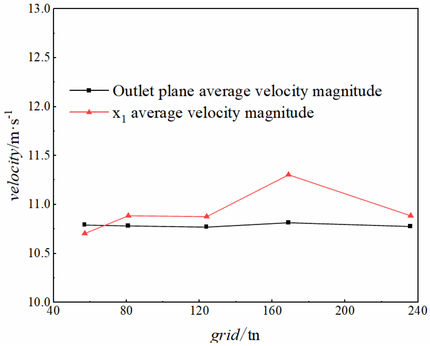
To ensure the accuracy and reliability of the numerical simulations, a rigorous grid independence study was conducted. The computational mesh was refined multiple times to evaluate the influence of mesh resolution on the simulation results. The computational mesh was created automatically, with the outlet dimensions adjusted and locally refined to improve accuracy. Figure 4 presents the outlet average velocity profiles and the corresponding mean velocities along the x₁ axis as the number of grid cells increases.

The average outlet velocity exhibits significant fluctuations along the centerline x₁ when the grid number is approximately 180 w. The remaining numerical discrepancies are minimal. To ensure computational stability and solution convergence, a grid size of 80,000 was adopted for the simulations.

Simulation is carried out by both transient and steady state methods, in which the steady state is iterated 600 times and the transient is set to have a step size of 1 s, with a total time of 600 s, resulting in results as shown in

Table 1. Base model 0.1 MPa~0.5 MPa transient and steady state data.

Inlet Pressure/MPa		0.1	0.2	0.3	0.4	0.5
x1 average velocity/(m/s)	Transient	11.18	15.81	19.35	22.34	24.99
	Steady state	11.18	15.81	19.34	22.33	24.96
Outlet average velocity/(m/s)	Transient	10.78	15.26	18.70	21.59	24.15
	Steady state	10.78	15.26	18.70	21.59	24.14
Outlet flux/(kg/s)	Transient	32.24	45.64	55.91	64.59	72.23
	Steady state	32.25	45.64	55.90	64.57	72.20

and

Table 2. Base model 0.6 MPa~1 MPa transient and steady state data.

Inlet Pressure/MPa		0.6	0.7	0.8	0.9	1
x1 average velocity/(m/s)	Transient	27.38	29.56	31.55	33.48	35.28
	Steady state	27.34	29.52	31.57	33.48	35.28
Outlet average velocity/(m/s)	Transient	26.47	28.59	30.54	32.40	34.17
	Steady state	26.78	28.57	30.55	32.40	34.15
Outlet flux/(kg/s)	Transient	79.17	85.52	91.33	96.92	102.20
	Steady state	79.11	85.44	91.37	96.92	102.16

When simulation is carried out by the two methods of steady state and transient, the average velocity along the outlet centerline can be observed, and they can be basically ignored. Therefore, it can be seen that the error exhibited by the two methods is small. Since the steady state can save time, the steady state is used in this paper for simulation and result analysis.

3. Results

3.1. Basic Model Analysis

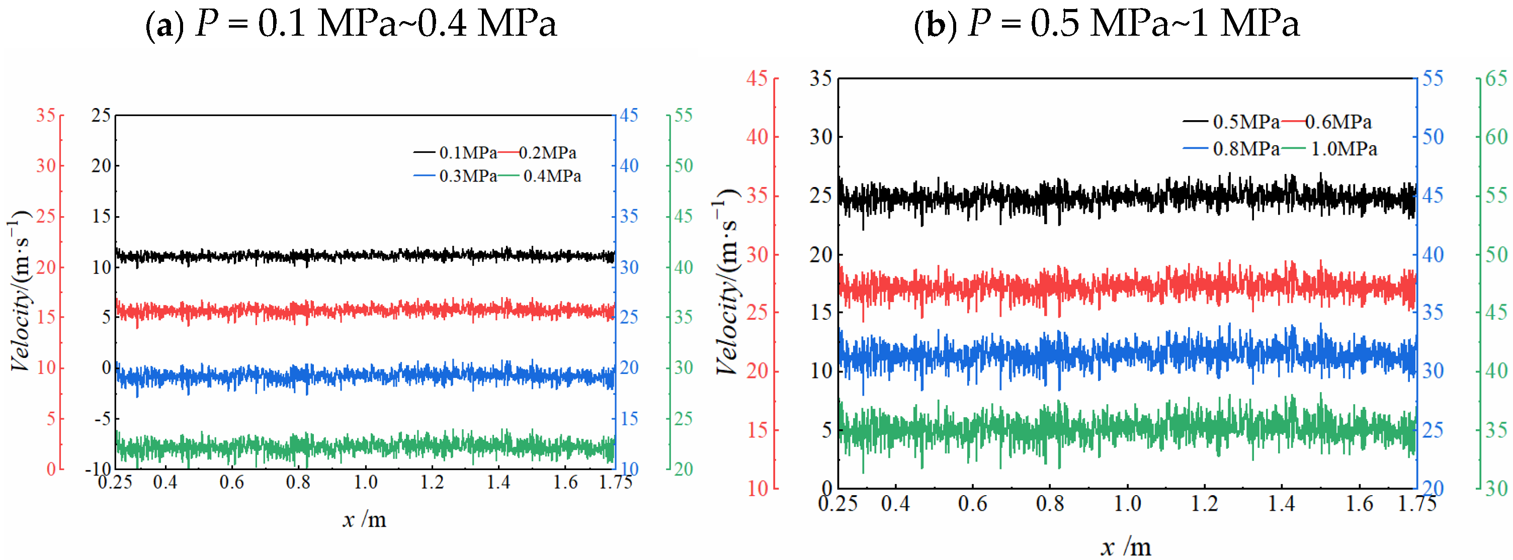
The following figure shows the analytical plot of the base model with pressure change results. Figure 5 shows the velocity fluctuation graph on the slot centerline x₁ under the inlet pressure of 0.1–1 MPa. As seen from the figure, the velocity increases significantly as the inlet pressure increases, and the velocity fluctuation also increases. It can be clearly seen through the graph that there is a concave decrease in the velocity from high to low in the region to the right of x = 0.25 mm, and the velocity fluctuation is larger in this region and more obvious with the increase in pressure. In the middle region, it can be seen that the fluctuation pattern of the curve is only different in numerical size, and the overall difference in the curve is located in the region of x = 0.8 m and x = 1.2–1.6 m, and this region will not change with the pressure change. Therefore, the results suggest that the velocity fluctuation pattern along the slot outlet centerline x₁ is minimally affected by pressure variations.

In summary, the change in pressure parameters has a small effect on the trend of the velocity profile, so only the 0.5 MPa results are taken for the analysis of the velocity profile after the subsequent structural changes.

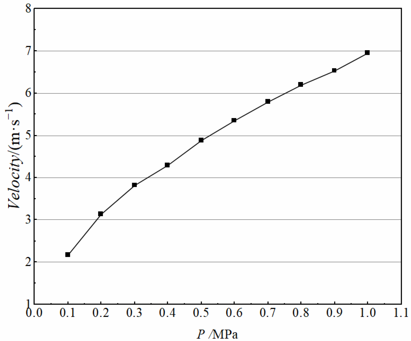
Figure 6 shows the velocity difference curves on x₁ at the outlet center of the slit for inlet pressures of 0.1–1 MPa. From the figure, it can be seen that the velocity difference on x₁ increases with the increase in inlet pressure, and it can be observed that the increase in the difference is significant and larger than the increment in the rest of the stages at 0.1–0.2 MPa; the minimum increment is in the section of 0.3 MPa~0.4 MPa, and the increment decreases slowly between 0.4 MPa and 0.9 MPa, and then increases significantly in the section of 0.9–1 MPa, increasing significantly at 0.9–1 MPa.

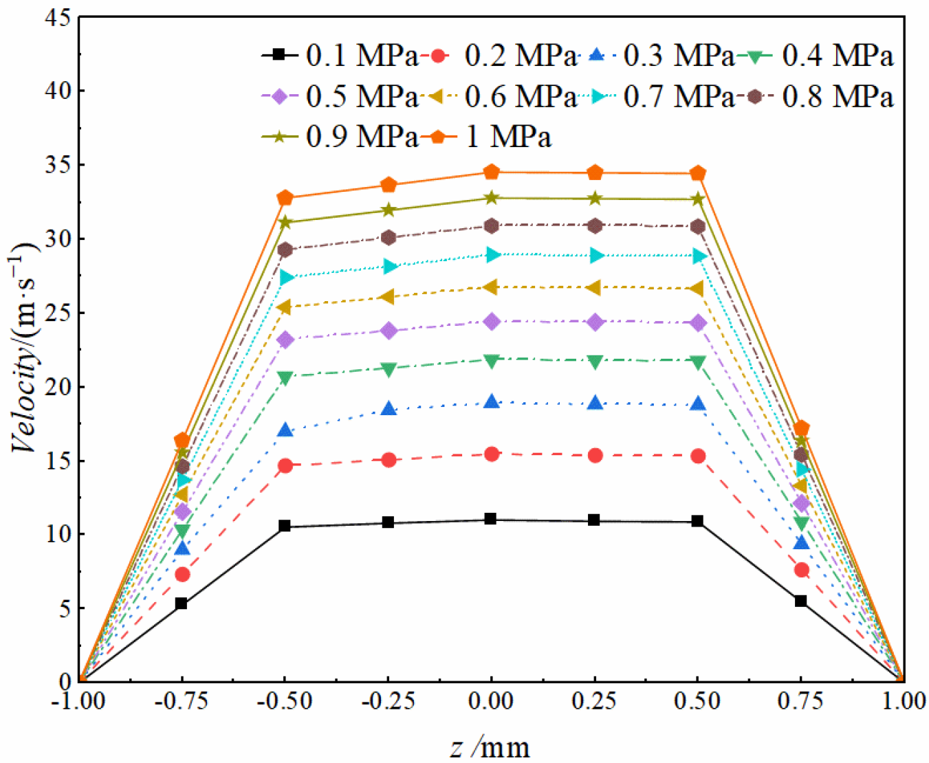
Figure 7 shows the velocity distribution curve on the length direction centerline z1 when the inlet pressure of the slit outlet is 0.1–1 MPa. As seen from the figure, the velocity profile on z₁ is isosceles trapezoidal in shape, in which the velocity of the upper bottom edge of the 0–0.5 mm section is slightly higher than that of the −0.50 mm section, and the highest velocity is found at z = 0 mm; the velocity difference between 0 mm and 0.5 mm is small, while the symmetric region shows a sloping increase; with the increase in pressure up to 0.6 MPa, the velocity of the center is higher than that on the right side, and the slope trend of the symmetric region is also more obvious. As the pressure increases to 0.6 MPa, the center velocity is higher than the right velocity, and the slope trend of the symmetrical region is more obvious.

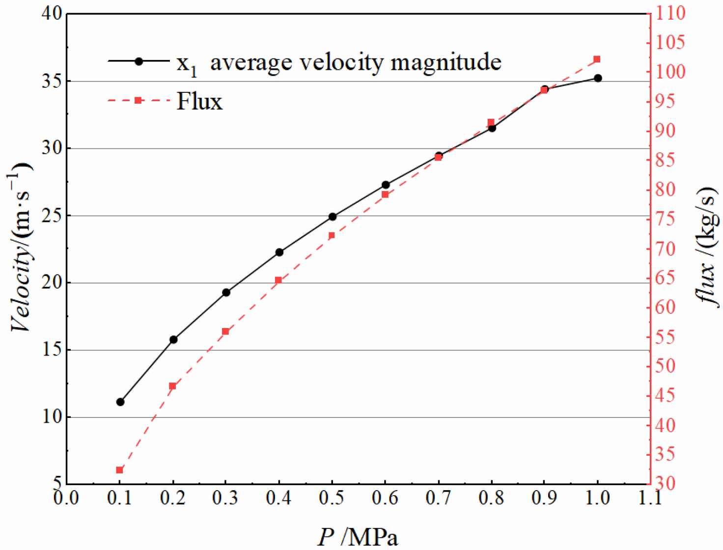
Figure 8 shows the curves of the average velocity magnitude on the outlet centerline x₁ versus the outlet flux when the inlet pressure is 0.1–1 MPa. From the figure, it can be seen that the overall trend of the outlet center velocity increases with the increase in inlet pressure, in which the increase between 0.1 MPa and 0.8 MPa decreases sequentially, and the increase between 0.8 MPa and 0.9 MPa increases, but continues to increase up to 1 MPa, the increase decreases again. The outlet flux law, on the other hand, is basically the same as the outlet center velocity increase law, which increases with the increase in inlet pressure and decreases sequentially. In summary, the change in pressure parameters has less influence on the trend of the velocity profile, so the velocity profile after the subsequent structural change only takes 0.5 MPa as the result for analysis.

3.2. Analysis of the Impact of Structural Changes on x₁

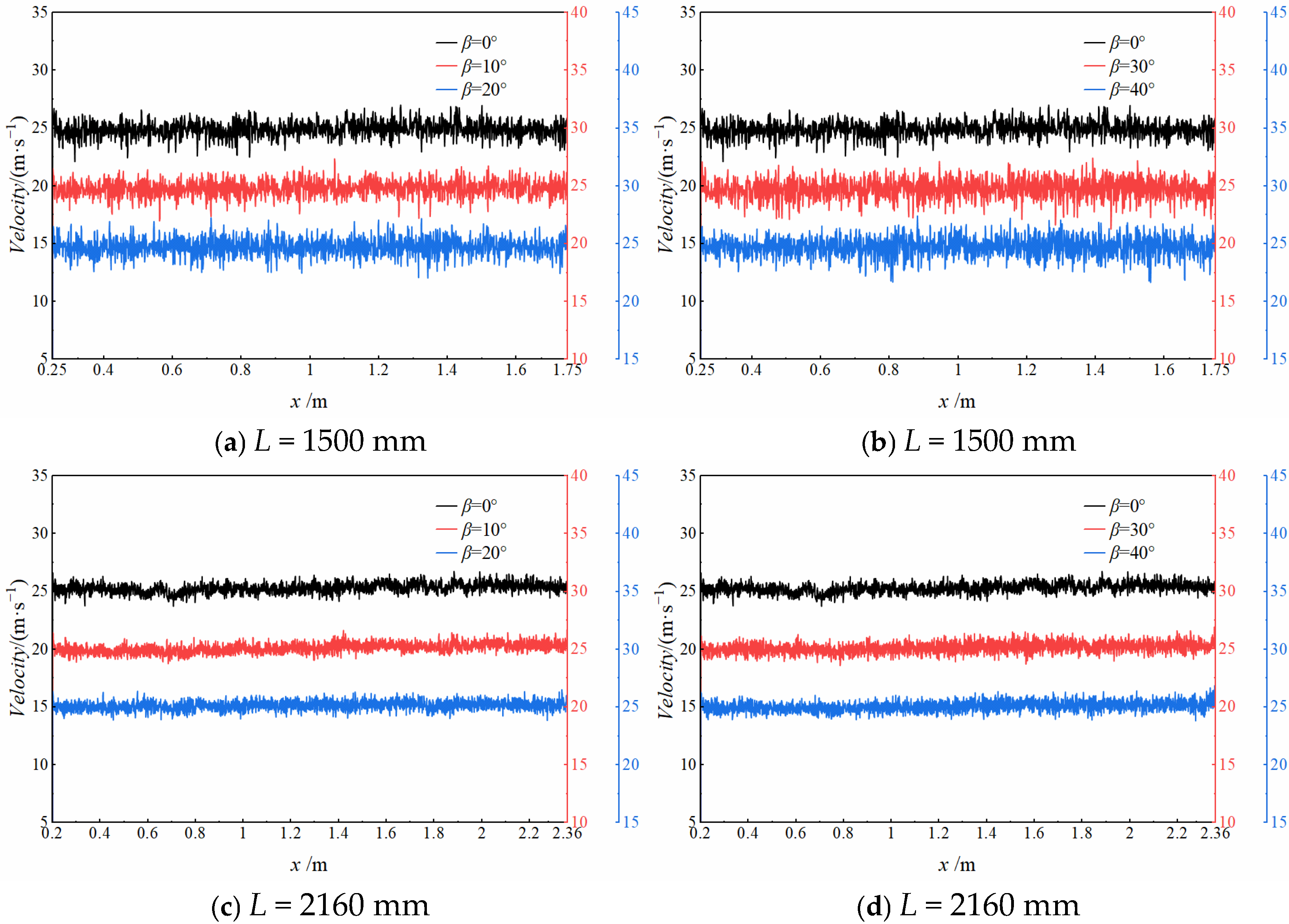
Figure 9a,b shows the velocity curves in the length direction of the center of the slit outlet when the inclination angle of the diverter hole β changes. From the figure, it can be seen that when β increases from 0° to 10°, there is no obvious change in the velocity in the direction of the center length of the slot outlet, but for β between 20° and 40° it can be seen that the velocity fluctuation increases significantly; from Figure 9c,d can be seen that with the increase in β, the size of the velocity fluctuation on the x₁ has no obvious change; β = 10° and β = 20° when there is no obvious stage of descent and ascent of the two sides of x₁. Figure 9a,c and Figure 9b,d show that comparing the slit outlet length of 1500 mm and 2160 mm, which are two sizes of the outlet, the diverter orifice inclination angle β has less effect on the velocity fluctuation in the direction of the center length of the slot outlet when the slot outlet length is 2160 mm.

In order to further analyze the impact of the angle β on the fluctuation in the slit outlet velocity, the mean (mean), fluctuation range (range), and mean absolute deviation (MAD) of the gap outlet velocity are shown in

Table 3. x₁ Velocity fluctuation data table when the diversion hole inclination angle changes.

Parameter	Mean	Range	MAD
L = 1500 mm, β = 0°	24.9073	4.8827	0.4810
L = 1500 mm, β = 10°	24.8023	5.3510	0.4999
L = 1500 mm, β = 20°	24.7487	5.1936	0.5441
L = 1500 mm, β = 30°	24.7724	6.1467	0.6282
L = 1500 mm, β = 40°	24.7526	5.7435	0.6137
L = 2160 mm, β = 0°	25.2920	2.9916	0.3160
L = 2160 mm, β = 10°	25.1102	3.3174	0.3222
L = 2160 mm, β = 20°	25.1334	2.6505	0.2907
L = 2160 mm, β = 30°	25.1337	4.7679	0.3405
L = 2160 mm, β = 40°	25.0541	3.1288	0.3190

. For the outlet length of 1500 mm, both the range and MAD values are significantly higher than those of the 2160 mm outlet, indicating that the shorter outlet is more sensitive to variations in the diverter hole inclination angle β. The mean velocity remains nearly unchanged across all operating conditions, indicating that the inclination angle beta has little influence on the average flow rate. In terms of fluctuation behavior, the L = 1500 mm outlet exhibits a non-monotonic variation with increasing beta, with more pronounced and irregular growth in fluctuation intensity at larger inclination angles. In contrast, the L = 2160 mm outlet shows consistently lower and less variable range and MAD values, suggesting that a longer outlet length can effectively suppress the velocity fluctuations induced by changes in beta.

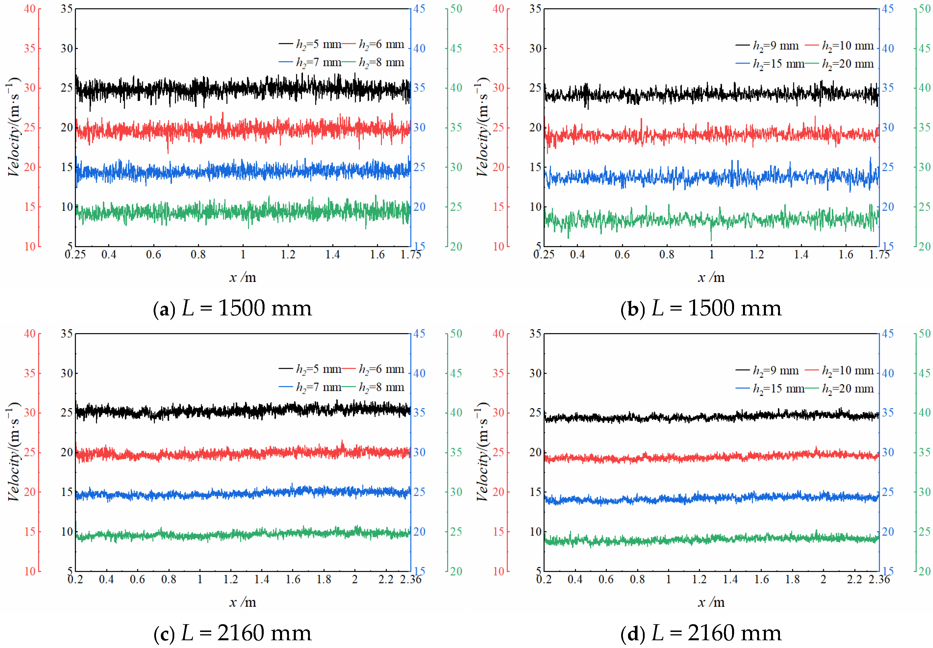
Figure 10 shows the velocity fluctuation curves of the x₁ upper jet under different slit heights h₂; from Figure 10a,b, it can be seen that the velocity fluctuation has a tendency to decrease with the increase in h₂. From Figure 10c,d, it can be seen that when h₂ is increased from 5 mm to 6 mm, the velocity fluctuation change is not obvious; when h₁ is increased to 7 mm, it can be seen that the velocity fluctuation is obviously reduced; between h₁ = 7 mm and 20 mm, the velocity fluctuation has no obvious change. From Figure 10a,c, it can be seen that in Figure 10b,d, the velocity fluctuation in the jet when the slit length is 2160 mm is generally smaller than that when the slit length is 1500 mm; the same point is seen when the height of the slit is increased to 9 mm, which causes the height of the slot to continue to increase; there is no obvious effect of reduction in the velocity fluctuation in the jet on x₁.

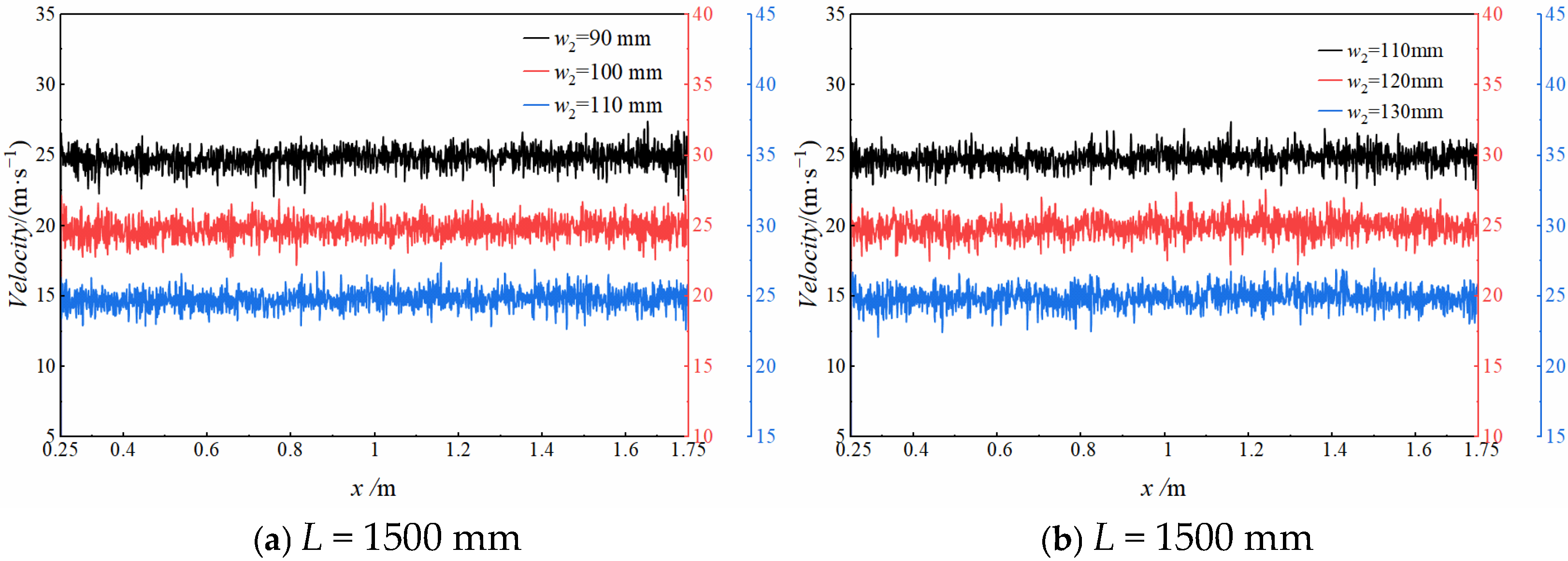
Figure 11 shows the jet velocity fluctuation curves on x₁ with different tank widths w₂ when the slot lengths are different. From Figure 11a,b, it can be seen that with the increase in the water tank width w₂, the size of the velocity fluctuation in the middle region of the x-direction does not change significantly; when w₂ = 110 mm and w₂ = 120 mm, it can be seen that the velocity of x₁ is on both sides of the unobvious rise-and-fall region, which is conducive to reducing the velocity difference between the two sides.

Table 4. x₁ velocity fluctuation with groove height variation.

Parameter	Mean	Range	MAD
L = 1500 mm, h2 = 5 mm	24.9073	4.8827	0.4810
L = 1500 mm, h2 = 6 mm	24.7564	5.6016	0.4682
L = 1500 mm, h2 = 7 mm	24.5213	4.0571	0.4187
L = 1500 mm, h2 = 8 mm	24.4321	4.3527	0.4713
L = 1500 mm, h2 = 9 mm	24.2217	3.6708	0.3793
L = 1500 mm, h2 = 10 mm	24.1387	4.7425	0.3887
L = 1500 mm, h2 = 15 mm	23.7553	4.4119	0.4335
L = 1500 mm, h2 = 20 mm	23.4189	4.6525	0.4469
L = 2160 mm, h2 = 5 mm	25.2934	2.9916	0.3160
L = 2160 mm, h2 = 6 mm	24.9140	2.994	0.2911
L = 2160 mm, h2 = 7 mm	24.8804	2.4177	0.2666
L = 2160 mm, h2 = 8 mm	24.7060	3.7317	0.2426
L = 2160 mm, h2 = 9 mm	24.5358	2.4198	0.2367
L = 2160 mm, h2 = 10 mm	24.4718	2.5632	0.2484
L = 2160 mm, h2 = 15 mm	24.2325	2.5936	0.2499
L = 2160 mm, h2 = 20 mm	24.0601	2.4883	0.2396
L = 1500 mm, w2 = 90 mm	24.8168	5.5706	0.4727
L = 1500 mm, w2 = 100 mm	24.8025	4.9508	0.5027
L = 1500 mm, w2 = 110 mm	24.8045	4.7413	0.4575
L = 1500 mm, w2 = 120 mm	24.9027	5.3396	0.5100
L = 1500 mm, w2 = 130 mm	24.9073	4.8827	0.4810
L = 2160 mm, w2 = 90 mm	25.2177	2.9497	0.3459
L = 2160 mm, w2 = 100 mm	25.2355	3.4738	0.3394
L = 2160 mm, w2 = 110 mm	25.2189	2.9091	0.3326
L = 2160 mm, w2 = 120 mm	25.2490	2.6918	0.3242
L = 2160 mm, w2 = 130 mm	25.2934	2.9916	0.3160

quantitatively illustrates the velocity fluctuation characteristics of the x₁ jet shown in Figure 10 and Figure 11. The slit height h₂ has a pronounced influence on the mean jet velocity. For both waterway lengths of 1500 mm and 2160 mm, the mean velocity decreases consistently as h₂ increases, indicating that a larger slit height weakens jet momentum. In contrast, the variation in velocity fluctuations with h₂ exhibits a clear dependence on the flow path length. Under the longer waterway condition (L = 2160 mm), both the range and MAD show a gradual decreasing trend with increasing h₂, suggesting that larger slit heights help to suppress velocity fluctuations and enhance flow stability.

3.3. Analysis of the Impact of Structural Changes on z₁

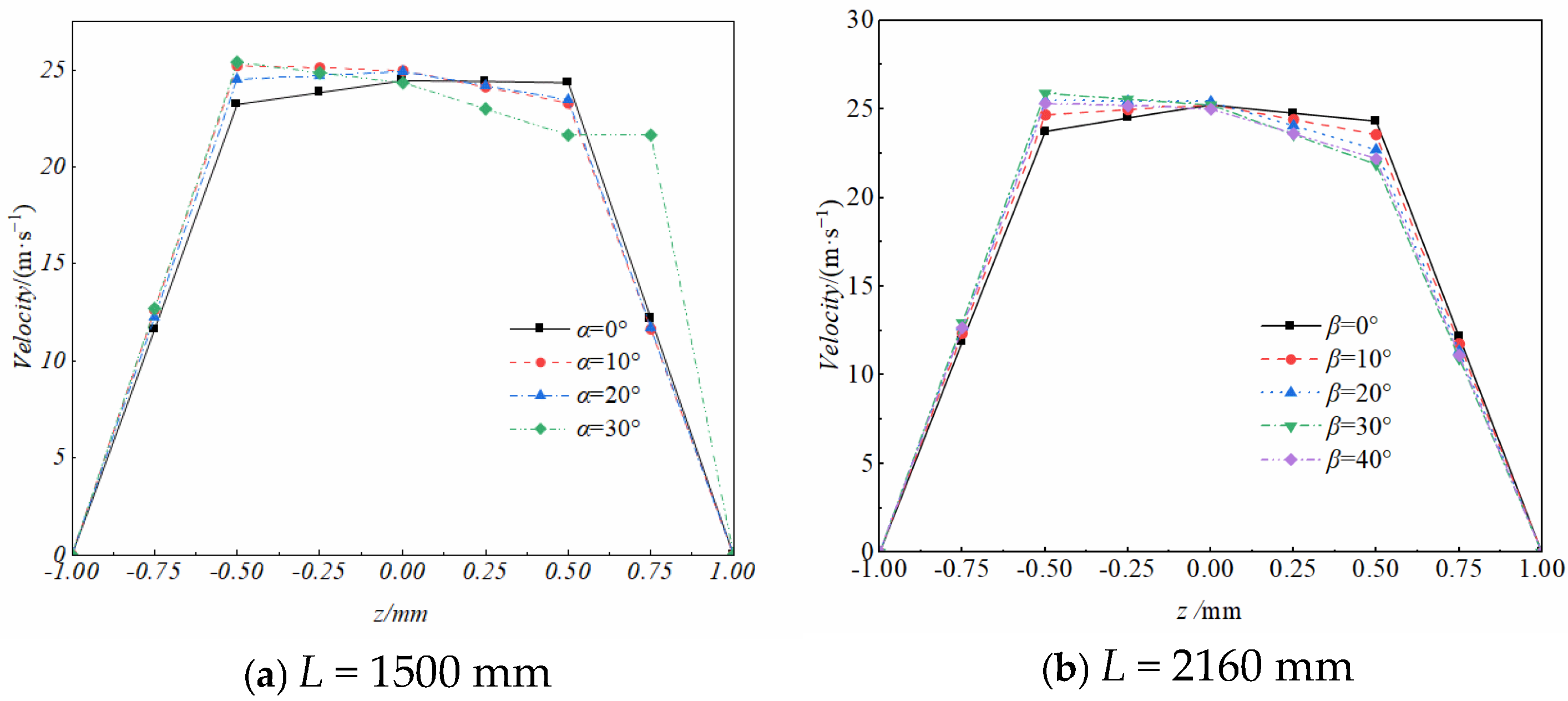
Figure 12 shows the velocity profile when the width direction z₁ of the slot outlet is changed with β. From Figure 12a, it can be seen that when the inclination angle of the diverter hole β increases, the velocity at the left end of the middle gently sloping area rises significantly, larger than that at the center and the right side, where a decreasing tendency is observed, which will cause the region with the highest velocity to be concentrated in the negative direction of z, resulting in the non-uniformity of the velocity distribution, which is detrimental to the enhancement of the jet’s agglomerative properties; when β = 30°, the velocity difference in the z direction is larger, with the velocity at z = 0.75. When β = 30°, the velocity difference in z direction is larger, and the velocity at z = 0.75 mm is much higher than the velocity at z = −0.75 mm; the distribution of jet velocity in the width direction z is also poorer than the center symmetry.

As seen from Figure 12b, when the inclination angle β of the diverter hole is increased, the jet velocity on the left side of the central uniform-velocity region is higher than that on the right side. And with the increase in β, the disparity in velocity between the left and right sides of the steady-velocity region becomes more pronounced, which is not conducive to improving the uniformity of velocity distribution. As seen from Figure 11, when β is changed, jet velocity at the center of the z direction when z = 0 mm has a small effect, which shows that the increase in the inclination angle of the diverter hole β does not improve the uniformity of jet velocity distribution in the width direction, but rather exacerbates the velocity difference between the two sides of the width center.

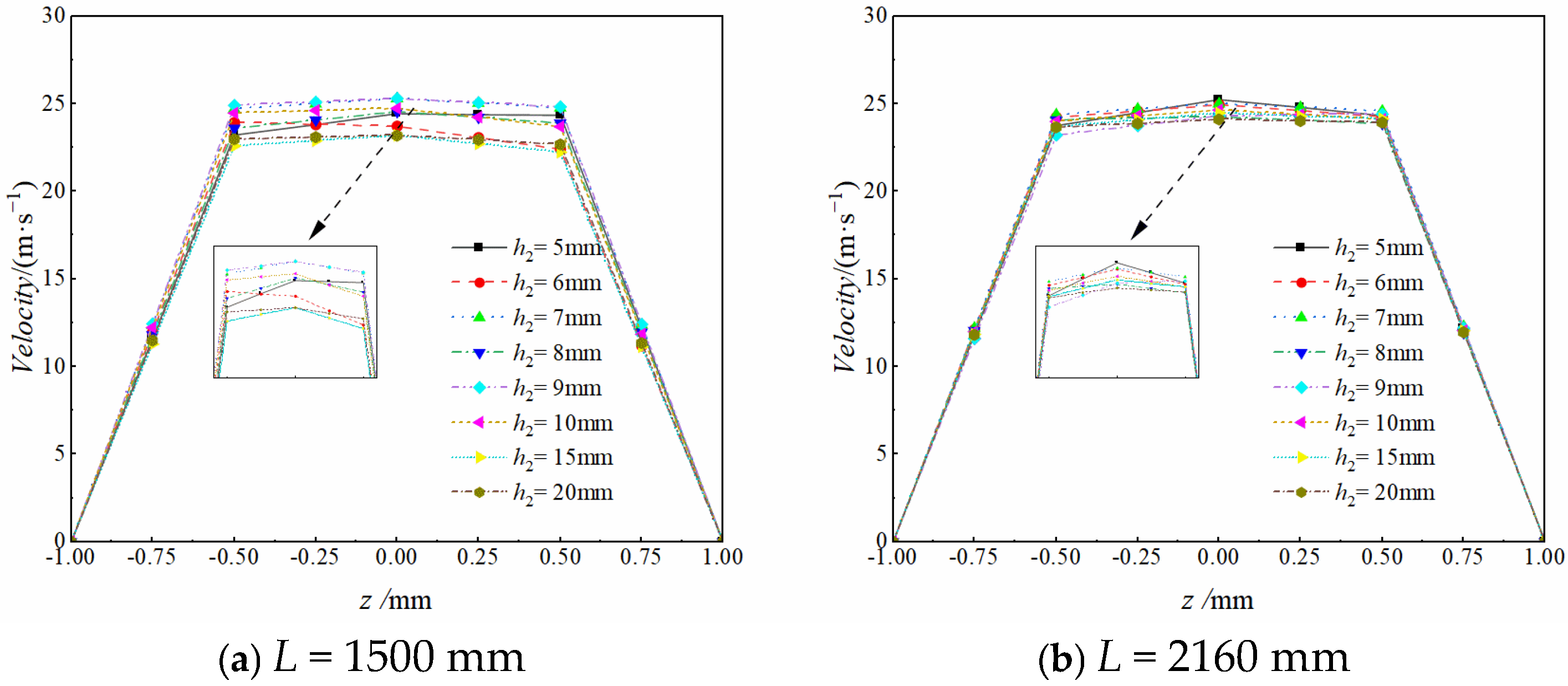
Figure 13 shows the jet velocity change curve on z₁ at different slot heights when the slot length is different; from Figure 13a, when the slot height h₂ = 6 mm, the jet velocity is the highest on the left side, and the velocity difference between the left and right sides is larger; in addition to h₂ = 6 mm, with the increase in h₁, the velocity difference decreases in the range of z = −0.75–0.75 mm, in which the differences between the left and right sides in this range are smaller when h₂ = 10 mm, h₂ = 15 mm, and h₂ = 20 mm, and the overall jet velocity is higher when h₂ = 9 mm, h₂ = 15 mm, h₂ = 20 mm; the difference between the left and right sides in this range is small, with h₂ = 9 mm, and the velocity of the two sides of the center is symmetrically distributed and the overall jet velocity is higher at this time. From Figure 13b, it can be seen that the jet velocity on z₁ shows a sharp trapezoidal trend in which the left side of the intermediate velocity plateau area is lower than the right side, and the velocity difference between the two sides of the intermediate velocity area of the jet decreases with the increase in the slot height h₂; it can be seen in the figure that with the increase in the slot height h₂, the velocity magnitude between the corresponding points of different slot heights varies less.

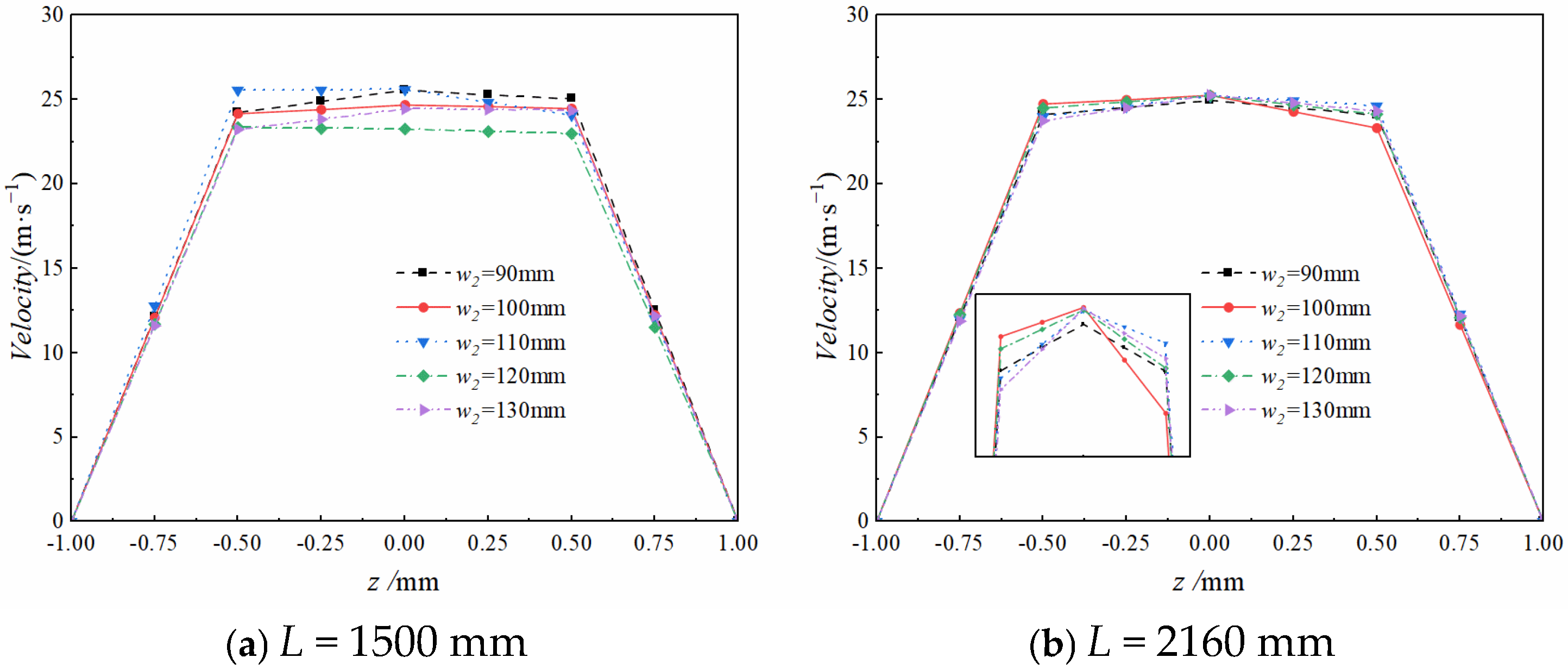
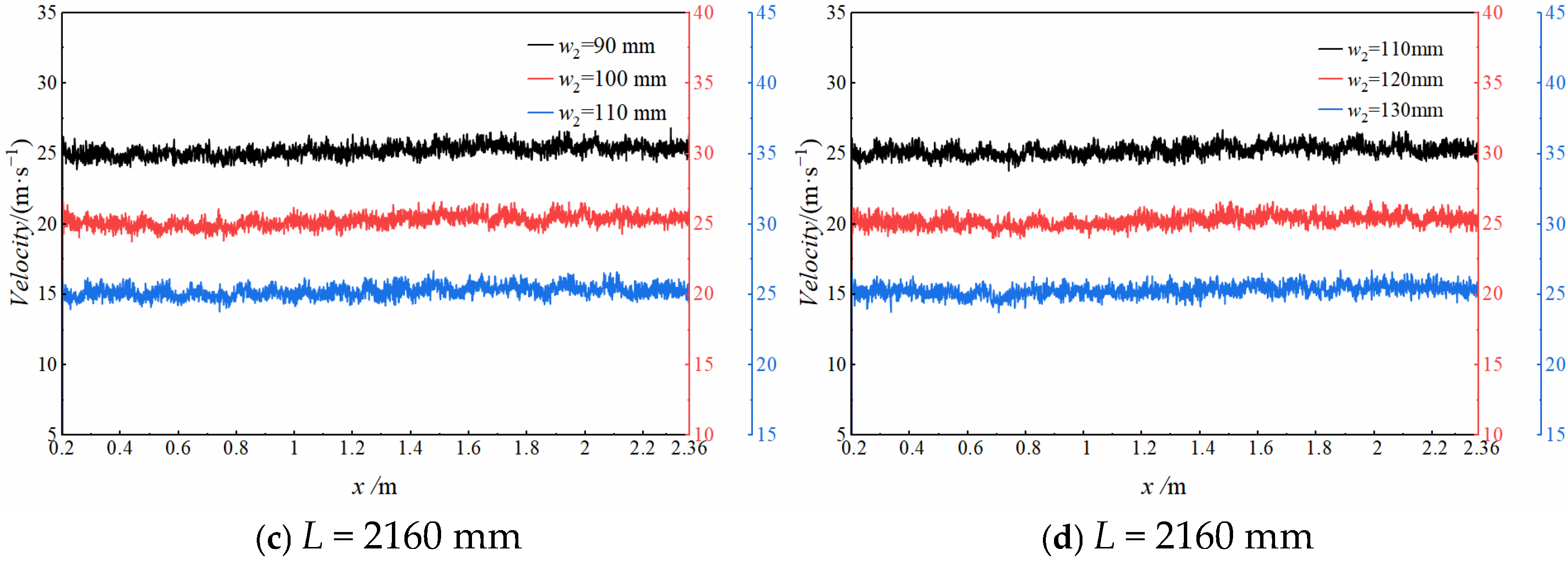
Figure 14 shows the velocity change curve on z₁ with different tank widths when the slot length is different; from the figure, we can see that in Figure 14a, the trend is the same when w₂ = 90 mm and w₂ = 130 mm, and the jet velocity shows a sharp trapezoidal trend with a low left and a high right; when w₂ = 110 mm and w₂ = 120 mm, it shows a trapezoidal trend with a high left and a low right and the left end of the gentle zone has a higher velocity than that in the center. w₂ = 100 mm has a symmetrical distribution of the velocity on both sides of the gentle zone, and the center velocity is slightly higher than that in the gentle zone. When w₂ = 100 mm, the flow exhibits symmetric velocity distribution across the uniform-velocity zone, and the velocity at the center is marginally higher than that on either side, which is conducive to the improvement in the uniformity of the velocity distribution in the gentle zone.

Figure 14b shows that when w₂ = 100 mm and w₂ = 120 mm, there is a high left side and low right side of the tip of the trapezoidal trend; with w₂ = 90 mm, w₂ = 110 mm, and w₂ = 130 mm, the middle region of the size of the jet velocity is at the low left and high right of the tip of the trapezoidal trend and the center of the velocity is the highest. As shown in Figure 13a, with the change in the tank width w₂, the difference in the size of the jet velocity on z₁ is more obvious, in which the jet velocity is the highest overall when w₂ = 110 mm, and the jet velocity is the lowest when w₂ = 120 mm; Figure 13b shows that when w₂ changes, the size of the jet velocity on z₁ is only slightly affected.

3.4. Analysis of the Effect of Different Structures on the x₁ Velocity Difference Curve

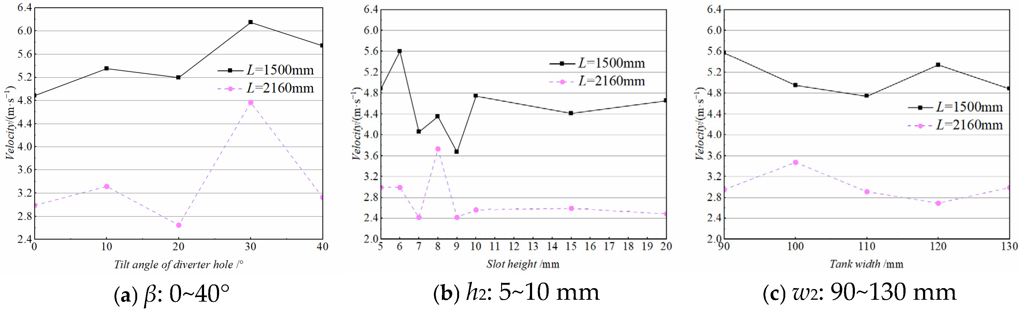
Figure 15 shows the jet velocity difference curves on the centerline x₁ of the slit outlet when the structure and the slit length are different. From Figure 15a, it can be seen that with the increase in the tilt angle β of the diverter hole, the jet velocity difference compared to the base model shows an overall increasing trend, in which β increases from 0 to 20°. The disparity in jet velocity initially grows and subsequently diminishes, and when β = 30°, the jet velocity difference reaches the maximum value, and β continues to increase to 40°; the jet velocity difference has a small decrease, but the jet velocity difference is still about 1 m/s higher than that of β = 0, which is about 1 m/s higher. It can be seen that when L = 1500 mm, the increase in the inclination angle of the diverter orifice is not favorable to reducing the velocity difference in the jet on x₁. When L = 2160 mm, with the change in the diverter hole tilt angle β, the jet velocity difference fluctuates greatly, in which β increases from 0 to 10°, the jet velocity difference of x₁ increases slightly, β continues to increase to 20°, and the jet velocity difference decreases significantly, in order to achieve the minimum jet velocity difference. When β increased to 30°, the jet velocity difference increased significantly for the maximum point; when β increased to 40°, the velocity difference decreased slightly, but when the overall is higher than 0° at x₁, the velocity difference is not favorable to 40°; when the velocity difference value decreases slightly, but the overall is higher than 0° at x₁, the jet velocity difference value is β = 20° when the velocity difference value is the smallest.

As shown in Figure 15b, the velocity difference is the largest when h₂ = 8 mm, and the velocity difference between h₂ = 5 mm and h₂ = 6 mm is basically unchanged; the velocity difference in the jet is basically the same when h₂ = 7 mm and h₂ = 9 mm, and the velocity difference in the jet is increased slightly when h₂ is increased to 10 mm; the velocity difference in the jet is basically unchanged when h₂ continues to increase to 20 mm. In summary, the increase in the slot height can effectively reduce the jet velocity difference on the slot nozzle outlet center x₁ and improve the uniformity of velocity distribution.

As shown in Figure 15c, the jet velocity difference of w₂ = 90 mm~110 mm decreases by about 1 m/s. When w₂ is changed from 110 mm to 120 mm, the jet velocity difference rises; when w₂ is changed from 120 mm to 130 mm, the velocity difference decreases slightly; among them, w₂ = 110 mm has the smallest value of velocity difference. It can be concluded that a reasonable choice for the width of the tank can reduce the velocity difference in the jet on x₁, and reduce the fluctuation in the jet velocity in the length direction. When the slot length L = 2160 mm, the tank width w₂ is changed from 90 mm to 100 mm, whereby w₂ = 100 mm~120 mm and the velocity difference is smaller; w₂ is changed from 120 mm to 130 mm and the jet velocity difference increases; when w₂ = 110 mm, velocity difference is the smallest; the slot length is L = 2160 mm, only when w₂ = 120 mm and when the jet velocity difference is smaller than the value of w₂ = 130 mm in the base model. In summary, the diverter orifice deflection angle, slot height, and tank width have a greater influence on the velocity extremes of x₁, but this parameter is also less affected as the overall performance with a slot length of 2160 mm is all better than the nozzle with a slot length of 1500 mm.

3.5. Simulation of Flux and x₁ Average Velocity

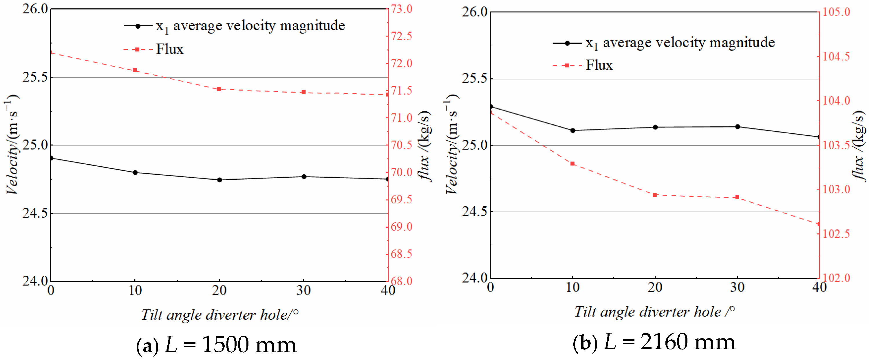
Figure 16 shows the variation curves of the mean velocity and outlet flux on x₁ as the diverter orifice deflection angle β varies. From Figure 16a, the results indicate that the average velocity and flux along x₁ exhibit a decreasing trend with increasing β.

It can be seen that the average velocity and flux on x₁ show a decreasing trend as β increases. Among them, the decreasing trend of average velocity and outlet flux on the slot outlet centerline x₁ is obvious when β = 10°~20°, while the change is smaller when β = 20°~40°. From Figure 16b, it can be seen that with the increase in β, the average velocity on x₁ shows an overall decreasing trend, and the size of the velocity is basically unchanged from β = 10° to 30°; the flux decreases with the increase in β and the decreasing trend is obvious, of which the decrease is the largest between β = 0° and 20°.

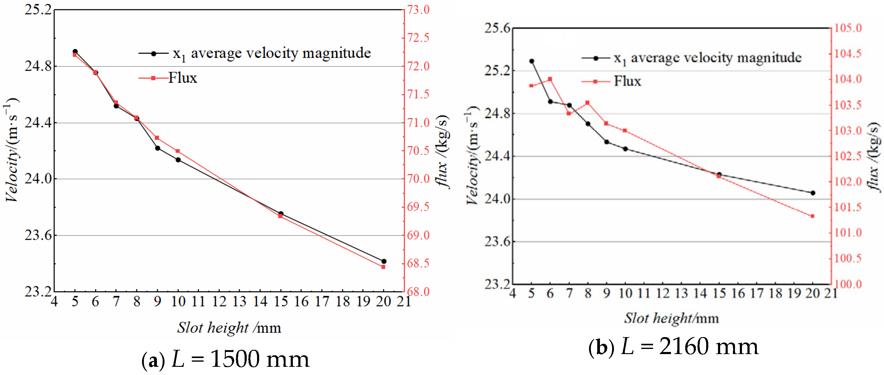
Figure 17 shows the curves of jet mean velocity and outlet flux on x₁ with respect to the slot height h₂ when the slot length is different. From Figure 17a, the results indicate that both the average jet velocity magnitude and the flux along x₁ exhibit a slight decline with increasing h₂. The decrease in jet mean velocity and outlet flux between slot height h₂ = 5 mm and 10 mm is larger than that of h₂ = 10–15 mm and h₂ = 15–20 mm. It can be seen from Figure 17b that the mean velocity of jet on x₁ decreases with the increase in the slot height, in which the magnitude and trend of the decrease in the mean velocity of the jet are similar to that of L = 1500 mm; when the slot height h₂ increases from 5 mm to 6 mm, the results indicate that the outlet flux exhibits a slight decline with increasing h₂. When h₂ varies between 5 mm and 6 mm, the outlet flux shows an increasing trend; from 6 mm to 7 mm, a decreasing trend is seen; from 7 mm to 8 mm, an increasing trend is seen; and from 8 mm to 20 mm, all show a decreasing trend. In summary, the increase in slot height can effectively reduce the velocity fluctuation in the direction of the jet length at the center of the outlet, such that the jet velocity difference in the middle region in the direction of the outlet width is reduced, which is conducive to the enhancement of velocity clustering, but the improvement in the uniformity of velocity distribution will result in a small decrease in the velocity at the same time.

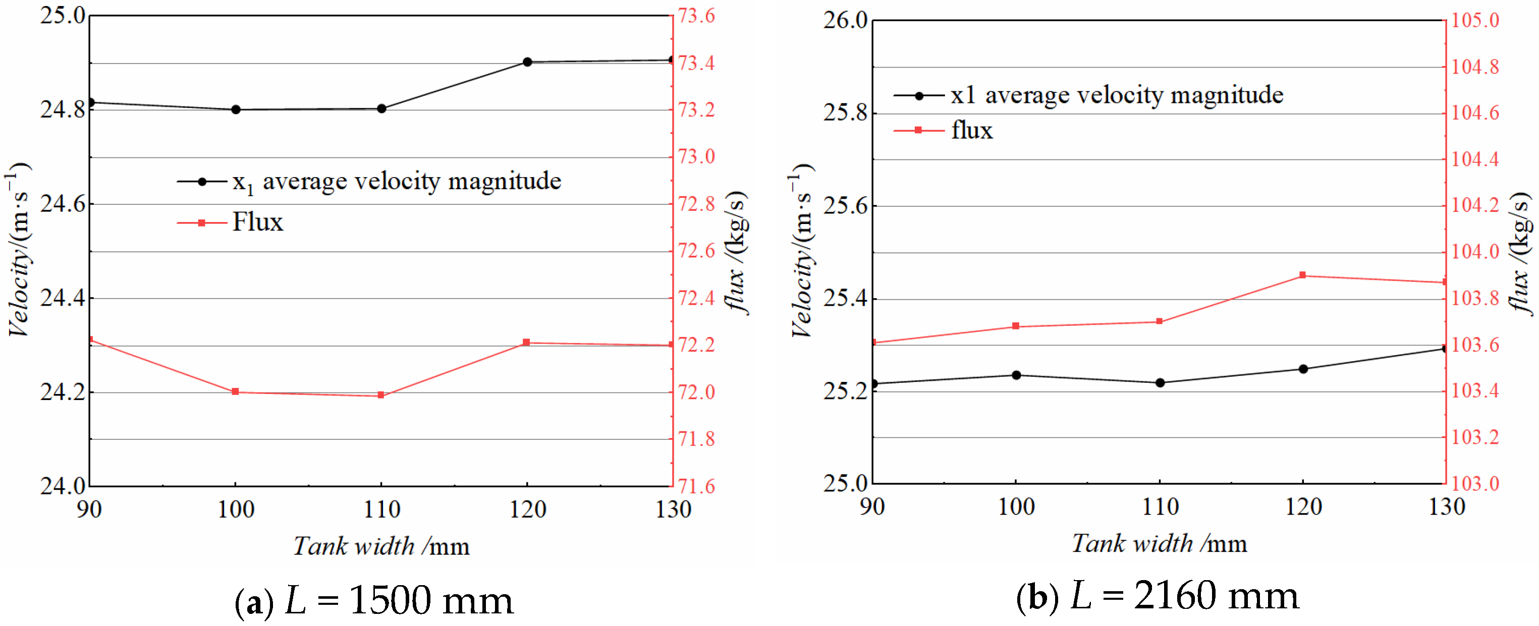
Figure 18 shows the curves of the mean velocity and outlet flux of the jet on x₁ as a function of the width of the tank w₂. From Figure 18a, it can be seen that with the increase in w₂, the average velocity and flux on x₁ decreases slightly between w₂ = 90 mm and 110 mm and increases slightly between w₂ = 110 mm and 130 mm. From Figure 18b, the average velocity of the jet on x₁ shows an overall increasing trend as w₂ increases, with a slight decrease when w₂ = 100 mm becomes w₂ = 110 mm. The flux increases slightly with the increase in w₂.

Although this study provides a detailed analysis of the flow characteristics in high-intensity cooling systems through three-dimensional numerical simulations and investigates the effects of different structural parameters, certain limitations remain. This study only considers a few representative geometries and operating conditions, while other factors, such as nozzle design variations and types of cooling media, were not explored. Future research could expand the range of these factors to investigate a broader design space, thereby improving the generality and applicability of cooling systems.

4. Conclusions

(1) The inlet pressure has minimal impact on the overall trend of the velocity fluctuation curve, and the velocity fluctuation increases with increasing pressure; the average velocity of the outlet surface of the slot and the average velocity of the center x₁ show an increasing trend, but the increase tends to be reduced, and when the inlet pressure continues to increase from 0.5 MPa, the reduction in the slope of the curve is more obvious.

(2) Through the analysis of the results of two sizes of slot nozzles, the velocity fluctuation, extreme value, flux, and other parameters of the outlet center are smaller when the slit length is 2160 mm than when it is 1500 mm.

(3) The proportional relationship between w₂ and ϕ₁ also has some influence on the flow characteristics, and within the range of parameters studied in this work, the flow uniformity is better when the relationship between w₂ and ϕ₁ is kept at 2/3.

(4) The effect of β, h₂ on the fluctuation in the outlet velocity fluctuation is more obvious; when β has a 0°~40° range increase, the outlet velocity fluctuation increases; when h₂ has a 5–20 mm range increase, the outlet velocity overall trend reduces; the effect of w₂ has less impact on the fluctuation. However, the increase in h₂ will make the velocity decrease, so the effect on speed should be paid attention to, while considering the improvement in uniformity.

References

1. Liu, X.; Xu, W.; Yang, K.; Du, L.; Wang, F.; Xia, Q.; Chen, J. Quench cooling of steel plates by reciprocating moving water jet impingement. Exp. Therm. Fluid Sci. 2024, 153, 111127. [Google Scholar] [CrossRef] [Scilit]
2. Zhang, D.; Ma, Z.; Yu, Z. Numerical Calculation of the Gradient of Velocity/Pressure under Impinging Submerged Circular Jets. J. Beijing Univ. Technol. 2000, 26, 63–67. (In Chinese) [Google Scholar]
3. Franco, G. Boiling Heat Transfer during Cooling of a Hot Moving Steel Plate by Multiple Top Jets. Ph.D. Thesis, University of British Columbia, Vancouver, BC, Canada, 2008. [Google Scholar]
4. Lytle, D.; Webb, B.W. Air Jet Impingement Heat Transfer at Low Nozzle-Plate Spacings. Int. J. Heat Mass Transf. 1994, 37, 1687–1697. [Google Scholar] [CrossRef] [Scilit]
5. Katti, V.; Prabhu, S.V. Experimental Study and Theoretical Analysis of Local Heat Transfer Distribution between Smooth Flat Surface and Impinging Air Jet from a Circular Straight Pipe Nozzle. Int. J. Heat Mass Transf. 2008, 51, 4480–4495. [Google Scholar] [CrossRef] [Scilit]
6. Narayanan, V.; Seyed-Yagoobi, J.; Page, R.H. An Experimental Study of Fluid Mechanics and Heat Transfer in an Impinging Slot Jet Flow. Int. J. Heat Mass Transf. 2004, 47, 1827–1845. [Google Scholar] [CrossRef] [Scilit]
7. Ashforth-Frost, S.; Jambunathan, K.; Whitney, C.F. Velocity and Turbulence Characteristics of a Semiconfined Orthogonally Impinging Slot Jet. Exp. Therm. Fluid Sci. 1997, 14, 60–97. [Google Scholar] [CrossRef] [Scilit]
8. Nirmalkumar, M.; Katti, V.; Prabhu, S.V. Local Heat Transfer Distribution on a Smooth Flat Plate Impinged by a Slot Jet. Int. J. Heat Mass Transf. 2011, 54, 727–738. [Google Scholar] [CrossRef] [Scilit]
9. Krishan, G.; Gallegos, R.K.B.; Sharma, R.N. Experimental Investigation of Thermal Characteristics of Slot Synthetic Jet Impingement on a Circular Cylinder: Free and Constrained Environment. Int. J. Heat Mass Transf. 2024, 230, 125770. [Google Scholar] [CrossRef] [Scilit]
10. Wu, H.J.; Zhang, S.W.; Zhang, Y.J. Numerical study on heat transfer characteristics of confined slot jet impingement heat transfer. Cryog. Supercond. 2021, 49, 37–43. (In Chinese) [Google Scholar]
11. Wang, M.B.; Wang, R.H.; Liu, X.Y. Numerical Simulation of a Semi-Confined Slot Turbulent Impinging Jet. Adv. Mater. Res. 2011, 268, 345–350. [Google Scholar] [CrossRef] [Scilit]
12. Chen, Q.G.; Xu, Z.; Zhang, Y.J. Numerical simulation of a semi-confined slot turbulent impinging jet. Chin. J. Appl. Mech. 2003, 2, 88–91. (In Chinese) [Google Scholar]
13. Yan, F.; Kong, W.; Jiao, H.; Peng, F.; Zhang, J. Flow Characteristics of Cylinders with Asymmetric Grooves: A Modeling and Experimental Study. J. Appl. Fluid Mech. 2024, 17, 1243–1260. [Google Scholar] [CrossRef] [Scilit]
14. Azimi, A.; Ashjaee, M.; Razi, P. Slot Jet Impingement Cooling of a Concave Surface in an Annulus. Exp. Therm. Fluid Sci. 2015, 68, 300–309. [Google Scholar] [CrossRef] [Scilit]
15. Zhu, D.M. Analysis of Slot-Jet Cooling Characteristics. Energy Metall. Ind. 2006, 25, 34–37. (In Chinese) [Google Scholar]
16. Liu, G.Y.; Zhu, D.M.; Zhang, S.J.; Li, M.W. Influencing Factors on Convective Heat Transfer of Impinging Slot Jet for Quenching. Chin. J. Eng. 2009, 31, 638–642. (In Chinese) [Google Scholar]
17. Singh, D.; Premachandran, B.; Kohli, S. Effect of Nozzle Shape on Jet Impingement Heat Transfer from a Circular Cylinder. Int. J. Therm. Sci. 2015, 96, 45–69. [Google Scholar] [CrossRef] [Scilit]
18. Meena, H.C.; Reodikar, S.A.; Vinze, R.; Prabhu, S.V. Influence of the Shape of the Orifice on the Local Heat Transfer Distribution between Smooth Flat Surface and Impinging Incompressible Air Jet. Exp. Therm. Fluid Sci. 2016, 70, 292–306. [Google Scholar] [CrossRef] [Scilit]
19. Royne, A.; Dey, C.J. Effect of Nozzle Geometry on Pressure Drop and Heat Transfer in Submerged Jet Arrays. Int. J. Heat Mass Transf. 2006, 49, 800–804. [Google Scholar] [CrossRef] [Scilit]
20. Soyama, H. Effect of Nozzle Geometry on a Standard Cavitation Erosion Test Using a Cavitating Jet. Wear 2013, 297, 895–902. [Google Scholar] [CrossRef] [Scilit]
21. Garimella, S.V.; Nenaydykh, B. Nozzle-Geometry Effects in Liquid Jet Impingement Heat Transfer. Int. J. Heat Mass Transf. 1996, 39, 2915–2923. [Google Scholar] [CrossRef] [Scilit]
22. Webb, B.W.; Ma, C.F. Single-Phase Liquid Jet Impingement Heat Transfer. In Advances in Heat Transfer; Hartnett, J.P., Irvine, T.F., Cho, Y.I., Eds.; Elsevier: Amsterdam, The Netherlands, 1995; Volume 26, pp. 105–217. [Google Scholar]
23. Dong, J.M.; Li, S.; Zhong, X.; Meng, R.X. Numerical simulation of submerged cavitating jet flow field with dual-throat nozzle. Fluid Mach. 2022, 50, 87–95. (In Chinese) [Google Scholar]
24. Wu, Z.; Wang, Y.; Zhang, S.; Lv, L.; Wang, W. Numerical Simulation of Cavitation Performance of Nozzles of Different Shapes. Fluid Mach. 2020, 48, 36–41. (In Chinese) [Google Scholar]
25. Li, C.; Shi, Y.; Yang, H.; Zhang, Y.; Yuan, G.; Li, Z.; Zhang, F. Heat Transfer Characteristics of Water Jet Impingement on High-Temperature Steel Plate by Angular Nozzle. Int. Commun. Heat Mass Transf. 2024, 151, 107243. [Google Scholar] [CrossRef] [Scilit]
Figure 1. Left-side view of the model.
Processes 13 03765 g001
Figure 2. Isometric projection of the model.
Processes 13 03765 g002
Figure 3. Outlet cross section x1, z1 position diagram.
Processes 13 03765 g003
Figure 4. Result of grid independence.
Processes 13 03765 g004
Figure 5. Base model centerline x1 velocity fluctuation curve.
Processes 13 03765 g005
Figure 6. Velocity difference curve on x1.
Processes 13 03765 g006
Figure 7. Velocity change curve of z1 with pressure.
Processes 13 03765 g007
Figure 8. Average velocity curve of centerline x1 with outlet flux.
Processes 13 03765 g008
Figure 9. Velocity fluctuation change curves of x1 with diversion hole tilt angle.
Processes 13 03765 g009
Figure 10. Velocity fluctuation change curves for x1 with slot height.
Processes 13 03765 g010
Figure 11. Velocity fluctuation change curve of x1 with tank width.
Processes 13 03765 g011aProcesses 13 03765 g011b
Figure 12. Velocity fluctuation curves of z1 at different tilt angles of the diversion hole.
Processes 13 03765 g012
Figure 13. Velocity change curve of z1 with slot height.
Processes 13 03765 g013
Figure 14. Velocity change curve of z1 with tank width.
Processes 13 03765 g014
Figure 15. Velocity difference curve under different structures.
Processes 13 03765 g015
Figure 16. Average velocity and outlet flux curves for x1 at different tilt angles of the diversion hole.
Processes 13 03765 g016
Figure 17. Average velocity and outlet flux variation curves for x1 with slot height.
Processes 13 03765 g017
Figure 18. Average velocity and outlet flux change curve for x1 with tank width.
Processes 13 03765 g018