Appendix A.1
The frequency bias factor
B is obtained by aggregating the frequency response characteristics of all participating resources on the system base. The equivalent droop coefficient
is defined as
where
is the rated capacity of the
i-th unit,
is the system base capacity, and
denotes the steady-state frequency–power conversion gain, with
for synchronous units and
for inverter-based resources such as wind, PV, and BESSs. The bias factor is then given by
where
D is the load damping constant.
In this study, the rated capacities of thermal, CAES, hydro, wind, PV, and BESS units are
MW, respectively, with a total system capacity of
MW. The droop coefficients are set as
,
, and
. The proportional coefficients of the synthetic inertia control strategy are set as
. Substituting these values into the above equation yields
Appendix A.7. Rationality and Sensitivity Analysis of Parameter Selection
The parameters listed in
Table A4 can be categorized into three groups:
- (1)
PPO algorithm parameters, including the actor network learning rate , experience horizon, clipping factor , entropy coefficient, discount factor, and trade-off coefficient;
- (2)
SETP algorithm parameters, which include all PPO parameters as well as the expert learning rate;
- (3)
Coefficients in the reward function, namely , , and .
PPO algorithm parameters
For the parameter configuration of the PPO algorithm, this study conducts systematic training and comparative analysis of several key hyperparameters to evaluate their impacts on the reward function and determine the optimal parameter combination listed in
Table A4.
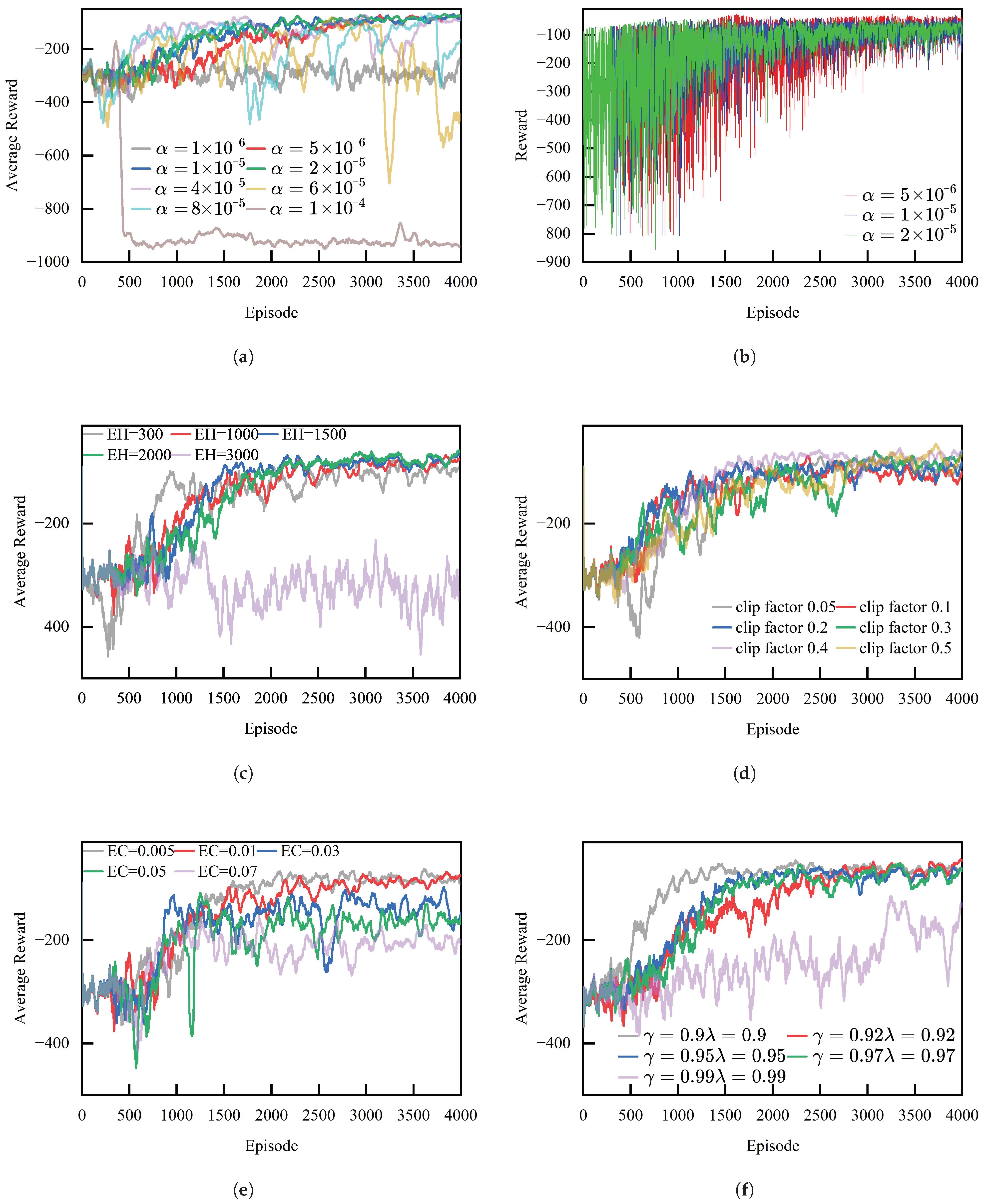
Figure A4a presents the smoothed reward curves of the PPO agent. It can be observed that a smaller learning rate (e.g.,
) leads to slower learning and a lower final average reward, while an excessively large learning rate (e.g.,
) causes excessive policy update amplitudes and results in policy collapse. A moderate learning rate (
–
) enables faster convergence to a better policy within fewer iterations.
Figure A4b also shows that the PPO agent achieves the smallest fluctuation in episode reward when
.
Figure A4c illustrates the effect of different experience horizon (EH) settings on the PPO training process. The results indicate that a large EH causes significant oscillations and keeps the episode reward at a relatively low level, while a small EH also leads to high fluctuations.
Figure A4d demonstrates the influence of different clipping factors on the PPO agent. The results show that an overly small clipping factor may restrict the policy optimization capability of the PPO algorithm, whereas a larger clipping factor performs better in the long run.
Figure A4e presents the effects of different entropy coefficients on PPO training. The results show that smaller entropy coefficients (0.005 and 0.01) achieve higher rewards, while larger entropy coefficients cause the agent to over-explore, resulting in a lower final reward.
Figure A4f shows the effect of
and
on the PPO agent. The results indicate that a smaller
focuses more on short-term rewards, enabling faster convergence but potentially limiting policy performance, while a larger
emphasizes long-term rewards, leading to slower convergence and a lower final reward.
SETP algorithm parameters
The SETP algorithm introduces an expert learning mechanism within the PPO framework, where the expert learning process also updates the parameters of the action network. Since the expert dataset contains approximately 64,800 samples, while the reinforcement learning process generates about 360,000 samples, and the quality of reinforcement learning data is relatively low in the early training stage, the network is updated five times during reinforcement learning but only once during expert learning, which is dominated by high-quality expert data. Therefore, in the expert learning stage, a higher learning rate is adopted for the actor network, while a lower learning rate is used in the reinforcement learning stage to balance the influence of the two types of data on network updates and maintain overall training stability.
Figure A4.
Comparison of average episode rewards of the PPO agent under different parameter settings. (a) Average episode reward under different learning rates. (b) Reward under different learning rates. (c) Average episode reward of the PPO agent under different experience horizons. (d) Average episode reward of the PPO agent under different clipping factors. (e) Average episode reward of the PPO agent under different entropy coefficients. (f) Average episode reward of the PPO agent under different discount factors and trade-off coefficients.
Coefficients in the reward function
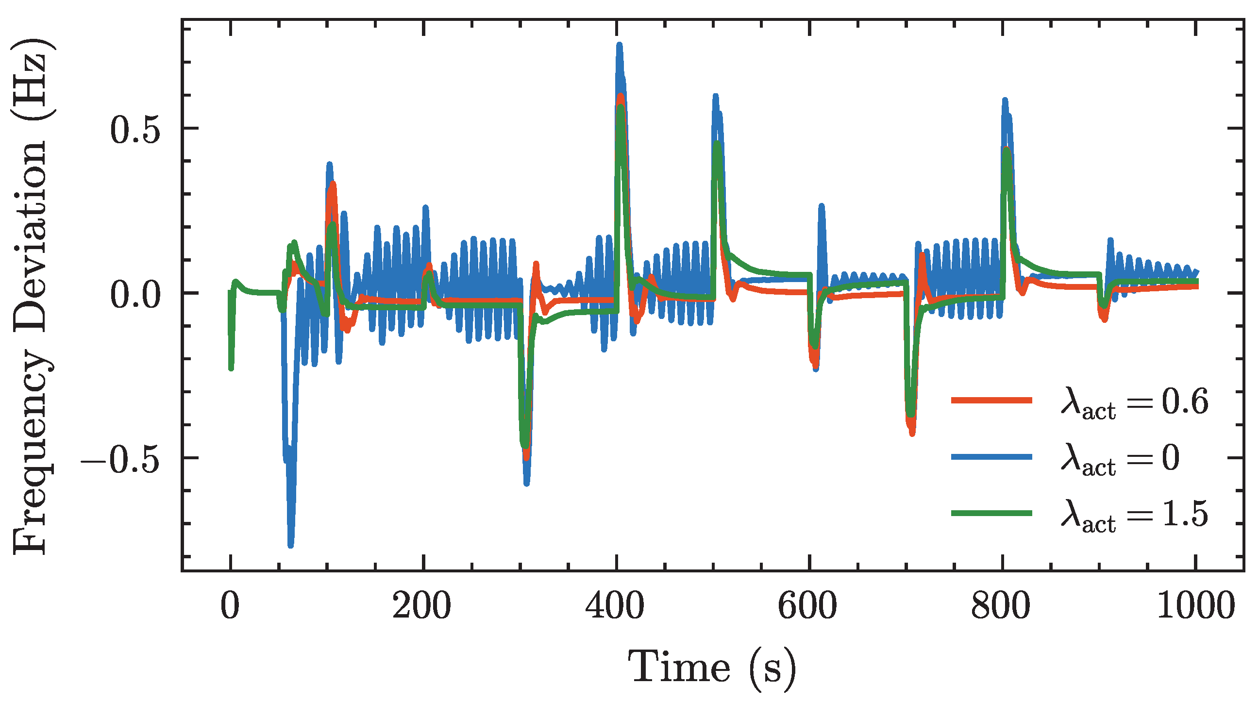
In the design of the reward function, the parameters , , and are used to adjust the penalty weights associated with frequency deviation, differences between consecutive actions, and regulation mileage, respectively. In the PPO algorithm, these three parameters are set as fixed values. As shown in the experimental results, when only is applied, the agent’s output actions tend to exhibit high-frequency oscillations. Introducing effectively suppresses these oscillations but makes the agent’s policy more conservative, reducing its responsiveness to frequency disturbances and thus affecting control performance. To balance control performance and output smoothness, a smaller coefficient for is selected through multiple experiments. The parameter corresponds to the penalty on control effort (i.e., regulation mileage). Increasing encourages the agent to suppress excessive action adjustments during training to avoid high regulation costs, thereby weakening its rapid response to frequency disturbances and degrading regulation performance. To highlight the superior control performance of the SETP algorithm compared with PPO, is set to zero in the PPO algorithm.
Figure A5.
The influence of different reward function coefficients on control performance.
Figure A5.
The influence of different reward function coefficients on control performance.
Selection of disturbance standard deviation:
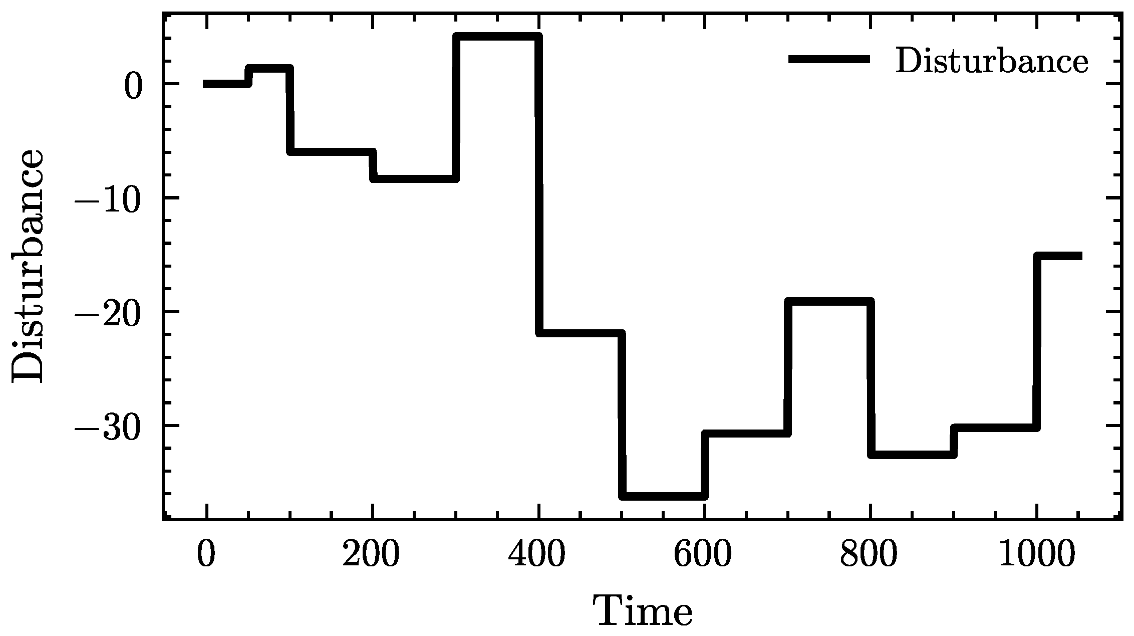
The should not be too large, as excessive volatility in the training environment may cause non-convergence or even collapse of the learning process and may also lead to excessively large frequency deviations, which are inconsistent with realistic operating conditions. On the other hand, if the disturbance intensity is too small, the environment becomes overly stable, leading to overfitting and poor generalization of the trained policy. Referring to the PI control strategy and after multiple trials, a reasonable range of disturbance intensities is determined in this study.
Selection of single-step disturbance amplitude:
Considering the scale of the clean energy base studied, the maximum frequency deviation is set to 0.6 Hz as the engineering threshold to ensure both frequency security and controllability. The threshold of the single-step disturbance amplitude
,
is constrained by this preset limit. As shown in
Figure A6, when the single-step disturbance amplitude is set to 0.021, the maximum frequency deviation is approximately 0.6 Hz.
Figure A6.
Simulation of different single-step disturbance amplitudes.
Figure A6.
Simulation of different single-step disturbance amplitudes.
Selection of the cumulative disturbance threshold:
The threshold for the cumulative disturbance , is set relatively loosely. On one hand, it should be sufficient to support stable operation during 5–10 consecutive upward or downward single-step adjustments. On the other hand, it must remain below the system’s maximum upward/downward regulation capability to prevent limit violations.

