Abstract
The increasing demand for monoclonal antibody (mAb) therapeutics has intensified the need for more efficient and consistent biomanufacturing processes. We present a data-driven, machine-learning (ML) approach to exploring and predicting upstream yield behavior. Drawing on industrial-scale batch records for a single mAb product from a contract development and manufacturing organization, we applied regression models to identify key process parameters and estimate production outcomes. Random forest regression, gradient boosting machine, and support vector regression (SVR) were evaluated to predict three yield indicators: bioreactor final weight (BFW), harvest titer (HT), and packed cell volume (PCV). SVR outperformed other models for BFW prediction (R2 = 0.978), while HT and PCV were difficult to model accurately with the available data. Exploratory analysis using sequential least-squares programming suggested parameter combinations associated with improved yield estimates relative to historical data. Sensitivity analysis highlighted the most influential process parameters. While the findings demonstrate the potential of ML for predictive, data-driven yield improvement, the results should be interpreted as an exploratory proof of concept rather than a fully validated optimization framework. This study highlights the need to incorporate process constraints and control logic, along with interpretable or hybrid modeling frameworks, to enable practical deployment in regulated biomanufacturing environments.
1. Introduction
Monoclonal antibodies (mAbs) are among the most successful biopharmaceutical products, with approved uses in oncology, autoimmune disorders, and infectious diseases [1], and global annual sales exceeding $120 billion as of 2017 [2]. As demand continues to rise, manufacturers face growing pressure to increase production efficiency and maintain quality under stringent regulatory standards. Upstream bioprocessing plays a critical role in determining final yield and product quality, as even minor deviations in cell culture conditions can significantly affect process outcomes [3].
Traditional process-optimization methods such as design of experiments (DoE) and mechanistic modeling have long supported process understanding and control [4]. However, these approaches struggle to capture the nonlinear and multivariable dynamics of large-scale mammalian cell cultures, where numerous interacting parameters create complex dependencies that are difficult to interpret [5].
Recent advances in data availability and computational power have driven the adoption of machine learning (ML) and related data-driven methods in bioprocessing [6]. ML models can reveal hidden patterns in process data that conventional statistical methods may overlook [7], complementing traditional tools for yield prediction, process control, and real-time decision-making using process analytical technologies (PAT) and manufacturing execution systems [8]. In parallel, hybrid modeling approaches that integrate ML with mechanistic insights have shown promise for improving interpretability and regulatory acceptance in continuous and automated manufacturing settings [9,10,11].
Despite this progress, the application of ML in Good Manufacturing Practice (GMP) environments remains limited by data heterogeneity, small batch numbers, and the black-box nature of many algorithms [12,13,14,15]. Mechanistic models, while interpretable, are constrained by the lack of quantitative descriptors for mammalian cell behavior and by difficulties in scaling to industrial systems [16,17,18]. Moreover, even well-designed mechanistic frameworks often fail to accurately capture real-world process variability, due to biological complexity, nonlinear responses, and incomplete experimental observability [19,20,21]. These factors make it challenging to achieve predictive precision and adaptability using mechanistic approaches alone.
As a result, purely mechanistic models are increasingly being complemented by ML-based and hybrid strategies that can learn directly from empirical data without requiring fully specified biochemical equations [22,23,24]. By identifying hidden correlations and nonlinear dependencies among process parameters, such data-driven frameworks can support more responsive and predictive control strategies in complex bioprocess environments. Furthermore, advances in deep learning have shown that models can automatically extract abstract data representations without prior mechanistic assumptions, providing powerful tools for uncovering latent structure in high-dimensional process datasets [25].
In this study, we apply a data-driven modeling framework to the upstream phase of mAb production using industrial-scale batch data provided by a global CDMO. The methodology combines exploratory data analysis (EDA) and machine learning regression to identify process parameters most strongly influencing harvested yield. By focusing on empirical patterns rather than predefined kinetic models, this work demonstrates how ML-based analysis of historical data can provide actionable insights for upstream optimization. The study highlights both the potential and limitations of ML for practical bioprocess improvement, emphasizing interpretability, data quality, and scalability as key considerations for future industrial implementation.
2. Materials and Methods
The dataset for this study was provided by a global CDMO specializing in large-scale mAb production. The objective was to leverage ML techniques to improve the upstream bioprocessing yield by analyzing historical batch records, identifying key process parameters, and applying predictive modeling and exploratory analysis strategies. This study adopted a statistical approach, leveraging ML models trained on historical batch data without relying on mechanistic or first-principles modeling. Its methodology encompassed several key steps, including data preprocessing, exploratory data analysis (EDA), ML model development, and process analysis. An overview of the methodology is provided in Figure 1.
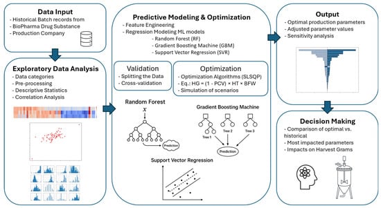
Figure 1.
Machine learning-based framework for yield improvement in the upstream bioprocess of monoclonal antibody production.
2.1. Process Overview
The production of mAbs involves several upstream processing steps that influence the final yield. The upstream phase primarily includes cell culture and expansion before the harvest step, when the drug substance is extracted for further downstream processing. In this study, the upstream process under analysis consists of the following key steps. The process begins with the thawing of a cryopreserved working cell bank vial of a recombinant Chinese hamster ovary (CHO) cell line expressing a monoclonal antibody, maintained under controlled, GMP-like conditions. The thawing rate and initial viability of cells can impact the subsequent expansion steps. After thawing, the cells are first expanded into small-scale shake flasks, providing an initial controlled environment for growth. Key parameters such as temperature, pH, and nutrient availability ensure that the cells reach target density before further scale-up. The culture is then transferred to a wave bag bioreactor, allowing for a greater volume of culture while maintaining proper oxygenation and mixing. Challenges at this stage include transfer timing and adaptation lag, which can affect the overall growth trajectory.
Following this, the upstream process includes several scale-up stages in bioreactors of increasing capacity, leading to the final production scale. Each transfer presents the risk of post transfer growth lag as cells adjust to the new environment. Proper transfer timing, cell viability, and inoculation density are critical to maintaining exponential growth during these stages. The final stage of upstream processing is carried out in a high-capacity production bioreactor, where the bulk of mAb production is achieved. Here, nutrient additions, pH regulation, and aeration control ensure that cells remain in a favorable production state. A key operational factor at this stage is the transfer window from the preceding bioreactor to the production bioreactor, which was investigated in this study for potential yield improvement. At the end of the cell culture phase, the drug substance is harvested through centrifugation and depth filtration. The final harvested yield is influenced by cell viability, viable cell density, and packed cell volume, which determine the efficiency of separation and product recovery. The upstream process flow is illustrated in Figure 2, which summarizes the sequence of unit operations from vial thaw to harvest and includes representative examples of process variables at each stage. These stages represent only the upstream phase of monoclonal antibody production analyzed in this study and do not include downstream purification steps.
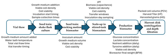
Figure 2.
Schematic representation of the upstream process of monoclonal antibody production using a recombinant Chinese hamster ovary (CHO) cell line. The diagram outlines the key upstream stages from vial thaw to harvest and includes representative examples of process variables at each stage.
Several process parameters influencing the final harvested yield were analyzed in this study. These included transfer timing, which impacts cell adaptation and growth consistency during the transition between bioreactors; cell growth lag, quantified as the time interval between inoculation and the onset of exponential growth based on viable cell density data; the adjustment of nutrient additions, such as tyrosine and glucose, which plays a critical role in maintaining cell viability and productivity; and process control constraints, including time windows for inoculation, incubation duration, and monitored variables, which influence process robustness.
2.2. Data Collection and Preprocessing
Historical batch records were used for the analysis. The dataset comprised three years of batch data from an industrial-scale upstream bioprocess covering various operational parameters, process variables, and batch outcomes.
Prior to the analysis, data preprocessing was performed to ensure consistency and reliability. Batches with missing critical values or incomplete production records were excluded. Additionally, nonrelevant variables, such as row counters and metadata unrelated to process outcomes, were removed. Outlier detection was conducted through exploratory data visualization, including the inspection of histograms, scatter plots, and box plots to identify extreme values. These potential outliers were subsequently analyzed to determine whether they resulted from genuine process deviations or data entry errors [23,26]. To maintain uniformity, numerical features were normalized to ensure comparable scales across different parameters.
The dataset was categorized into distinct groups based on their role in the bioprocess. For clarity, the terminology used in this study follows standard process-control conventions: “process inputs” denote adjustable operational settings; “monitored variables” represent measured process-state conditions; and “dependent variables” are the modeled yield outcomes.
- Dependent Variables (Yield Indicators): The primary output metric was harvested grams (HG), with packed cell volume (PCV), bioreactor final weight (BFW), and harvest titer (HT) serving as critical yield-determining factors.
- Process Inputs (Adjustable Process Variables): This group includes all controllable operational factors, such as growth medium addition, nutrient and tyrosine supplementation, inoculum weight, and time-based process parameters (e.g., incubation durations, sampling times, and transfer windows).
- Monitored Variables (Process-State Conditions): These variables were measured throughout the process but not directly adjusted. Key variables included pH, glucose, lactate, viable cell density (VCD), biomass capacitance, and aeration conditions.
After preprocessing, 65 batches were retained for analysis, containing 79 process inputs and 104 monitored variables. These cleaned and structured data served as the foundation for EDA and ML modeling.
2.3. Exploratory Data Analysis
Before applying ML models, EDA was conducted to assess the dataset’s structure, identify key trends, and detect potential data inconsistencies. The goal of this analysis was to understand the relationships between process parameters and yield outcomes and to establish a baseline for model development.
EDA was performed using descriptive statistics, correlation analysis, and visualization techniques [5,27]. Descriptive statistics were used to summarize the key variables, providing insights into the distribution of CPPs. Correlation matrices were generated to evaluate the relationships between process inputs, monitored variables, and dependent yield indicators. Heatmaps were employed to visualize the correlations between process parameters and harvested yield. Parameters showing negligible or inconsistent correlations with yield outcomes were excluded, while those exhibiting meaningful relationships were retained as candidate features. In addition, scatter plots and histograms were used to analyze parameter distributions across batches, helping identify potential trends or process inconsistencies.
EDA insights were used to guide feature selection and model development, ensuring that only the most relevant parameters were considered in the ML models. By examining correlations and variable distributions, EDA helped refine the input space for predictive modeling and improve model interpretability and performance.
2.4. Machine Learning Model Development
To build predictive models for bioprocess yield improvement, various ML techniques were employed in a statistical modeling framework. As this work employed a data-driven statistical methodology, no mechanistic representations of the bioprocess were incorporated. The models captured empirical relationships solely from historical process data. The goal of the model development was to identify key process parameters that significantly influenced production yield and to use these insights to improve future batch performance. Three regression models were implemented to predict the key yield indicators: HT, PCV, and BFW. The models included random forest (RF) regression, gradient boosting machine (GBM), and support vector regression (SVR). Each model analyzed one dependent variable at a time using a multivariate set of input features that included process inputs and monitored variables. While each regression model predicted one dependent variable (univariate output), the modeling framework operated within a fully multivariate input space encompassing process inputs and monitored variables. In ML practice, it is common to approach multivariate problems by training one model per output, particularly when the outputs differ significantly in behavior or predictive difficulty [28]. Therefore, while our modeling approach was technically univariate in structure, the overall framework reflected a multivariate modeling context.
RF was used to capture nonlinear relationships and feature interactions [29,30]. A grid search was applied to optimize hyperparameters, such as tree depth [31], the number of estimators, and the minimum sample split, while cross-validation (CV = 5) was used to evaluate model generalizability. GBM was selected for its ability to improve prediction accuracy by iteratively minimizing errors, using additive training of weak learners to focus on the residuals of prior models [32]. Hyperparameters such as learning rate, the number of estimators, and tree depth were tuned using GridSearchCV. Hyperparameter tuning was performed using GridSearchCV, which systematically evaluated multiple combinations of model parameters to identify the configuration yielding the highest cross-validated R2 score. For example, the grid included ranges such as: RF−number of trees (100–500), maximum depth (3–10), and feature sampling (‘sqrt’, ‘log2′); GBM—estimators (25–500), learning rate (0.005–0.05), and maximum depth (3–5); SVR—kernel (‘linear’, ‘rbf’), C (0.01–50), gamma (‘scale’, ‘auto’), and epsilon (0.01–0.15). The final configuration for each model corresponded to the best-performing combination under 5-fold cross-validation. SVR was implemented to model complex relationships with a kernel-based approach that maximizes margin tolerance while minimizing prediction error—a widely adopted method in nonlinear regression tasks [33].
The models were evaluated using coefficient of determination (R2) scores, which measure the proportion of variance explained; mean absolute error (MAE), which provides an average magnitude of prediction errors; and mean squared error (MSE), which gives higher weight to large deviations. These metrics are standard in model evaluation for continuous output predictions [34].
The training pipeline was designed to optimize the following objective function:
where HG (harvested grams) represents the total product mass obtained after harvesting (g), PCV (packed cell volume) is expressed as a fraction of total bioreactor volume (dimensionless), HT (harvest titer) is measured in grams of antibody per liter of harvest fluid (g/L), and BFW (bioreactor final weight) corresponds to the total liquid weight in the production bioreactor (kg or L, assuming 1 kg ≈ 1 L). This formulation captures that increasing bioreactor content (BFW) and antibody concentration (HT), while minimizing cell mass fraction (PCV), leads to higher overall product yield. This objective function was formulated as a process-informed composite metric representing the total harvested product mass, combining the effects of antibody concentration (HT), harvest volume (BFW), and the non-productive cell fraction (PCV).
HG = (1 − PCV) × HT × BFW,
After training and validating the models, an exploratory parameter-search framework was applied. Sequential least squares programming (SLSQP) [35] was used to maximize HG, subject to process constraints. Sensitivity analysis was performed to identify the most influential features of yield, ensuring that the optimization strategy focused on the most impactful process variables.
2.5. Output
The output of the ML models consisted of model-recommended production parameters and adjusted process variable values aimed at improving the final harvested yield. The predictive models generated estimates for BFW, HT, and PCV based on historical batch data and identified key process parameters that influenced these outcomes.
To determine the most impactful parameters, a feature importance analysis was conducted, ranking the input variables based on their contribution to yield improvement [29,36]. The optimization step utilized the best-performing model to recommend adjusted process conditions that would lead to an increase in HG.
Additionally, a sensitivity analysis was performed to evaluate how variations in the process inputs affected the yield [37]. This allowed for the identification of CPPs that had the greatest influence on production outcomes. The results of this sensitivity analysis provided insight into how specific parameter adjustments could improve process robustness and batch-to-batch consistency.
2.6. Decision-Making
After developing and validating the ML models, the next step involved leveraging the model predictions to support data-driven decision-making for upstream bioprocess improvement. The primary objective of this stage was to translate model insights into actionable process modifications that could enhance the production yield.
The decision-making framework was designed to compare historical process performance against the model-recommended parameter settings. This analysis focused on identifying the key process variables with the highest impact on the final HG. By assessing the influence of monitored variables and process inputs on yield outcomes, process engineers can make informed adjustments to enhance batch consistency and maximize production efficiency [23,38,39].
A comparative analysis was performed between the predicted recommended conditions and actual historical batch performance, including the following key steps:
- Parameter Adjustment Recommendations: The ML models identified critical factors that significantly impacted yield. These insights were used to propose recommended parameter settings.
- Impact Assessment: The sensitivity analysis results provided a quantitative measure of how changes in specific process variables would affect overall HG.
3. Results
3.1. Exploratory Data Analysis
EDA was conducted to understand the dataset structure, identify correlations between variables, and determine the key features for ML modeling. The primary objective of EDA was to filter out noninformative parameters, visualize trends, and assess feature distributions.
3.1.1. Feature Distribution and Variability Analysis
To analyze variability, histograms (Figure 3) were generated for all parameters, allowing for the identification of those with minimal variance across batches. Parameters showing little to no variation were excluded from further analysis, as they would not contribute meaningful insights to the predictive model. Figure 3 presents representative examples of these histograms for a subset of sixteen parameters, illustrating the general shapes of the normalized distributions and enabling visual comparison of variability and skewness across parameters.
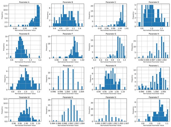
Figure 3.
Representative histograms of normalized process parameters showing their distributions across all batches. Parameter names have been anonymized and relabeled alphabetically (A–P) to maintain confidentiality while preserving comparative insight.
Variability was assessed visually from the parameter histograms and descriptive statistics. Parameters displaying nearly uniform or constant values across all batches were considered non-informative and excluded from further modeling. Additionally, normalization ensured comparability across parameters, enabling effective ML modeling.
3.1.2. Correlation Analysis
Following the initial screening, a comprehensive correlation analysis was performed to quantify the relationships among process inputs, monitored variables, and the dependent variables (PCV, BFW, and HT). Pearson correlation coefficients were calculated separately for these categories of independent variables, and correlation matrices were generated to identify the parameters most strongly associated with each dependent variable.
The top five parameters with the strongest correlations to each dependent variable are summarized in Table 1. The parameter names were generalized to preserve confidentiality while maintaining interpretability.

Table 1.
Top five process parameters most correlated with each dependent variable in the mAb production dataset used in this study 1.
The BFW showed notably strong correlations with key process inputs, such as tyrosine and nutrient additions, indicating potential for predictive modeling. In contrast, the correlation strength for HT and PCV was substantially lower, suggesting inherent complexity or nonlinear relationships requiring more advanced modeling methods. These insights guided subsequent feature engineering and the selection of parameters for ML model development.
3.1.3. Scatter Plot Analysis
Scatter plots were constructed to visually assess the relationships among important parameters and dependent variables. While correlation coefficients quantify linear relationships, scatter plots reveal potential nonlinear patterns, clustering, or outliers that may not be evident numerically. However, none of the parameters demonstrated a distinct, strong linear relationship with the dependent variables, as illustrated in Figure 4. This underscores the necessity for ML methods capable of capturing complex, nonlinear patterns.
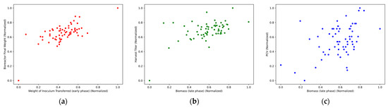
Figure 4.
Scatter plots of selected parameters. (a) Bioreactor final weight vs. inoculum transfer mass (early production phase); (b) Harvest titer vs. biomass level (late production phase); (c) Packed cell volume vs. biomass level (late production phase).
The scatter plots confirmed that no strong visual correlations existed between the independent and dependent variables. This finding supports the decision to apply nonlinear regression methods, such as RF, GBM, and SVR, to model the underlying relationships more effectively.
In addition, batch-to-batch variability was analyzed through visual distribution studies to assess the consistency and reliability of historical data as a foundation for modeling. The distribution analysis demonstrated that the process parameters remained consistent across historical batches, indicating stable operational conditions. This consistency validates the suitability of historical batch data for predictive modeling, as it suggests a reliable and well-controlled manufacturing process.
3.2. Machine Learning Model Performance
Predictive models were developed for the three key dependent variables (BFW, HT, and PCV). To model these variables, three regression models were implemented: RF, GBM, and SVR. Each model was evaluated using the R2 score, MAE, and MSE performance metrics. Feature engineering was applied to improve the models’ performance, with different combinations of parameters tested to assess their impact. As part of this process, feature importance rankings were extracted from each algorithm to quantify the contribution of individual process parameters to model predictions. These rankings guided the elimination of low-impact features and the construction of refined feature sets tailored to each output. By focusing on variables with the highest predictive relevance, the modeling pipeline was streamlined and better aligned with the underlying process dynamics.
After feature screening, approximately 40–50 parameters were retained for model training. The dataset of 65 historical batches was randomly divided into 80% for model training and 20% for testing. Within the training set, a 5-fold cross-validation approach was used for model validation and hyperparameter optimization, ensuring generalizable model performance. Following extensive model evaluation, the predictive performance of each model across all dependent variables is summarized in Table 2, which also highlights the best-performing configuration identified for each dependent variable.
Table 2.
Predictive performance of machine learning models for each dependent variable. The table summarizes R2 test scores and highlights in bold the best-performing model per dependent variable 1.
The SVR model that achieved the best predictive performance for BFW relied on a combination of timing and biological parameters. The most influential features included the inoculum transfer weight, biomass levels during early production, process duration metrics across sequential expansion phases, interbioreactor transfer timing, and cumulative sample times collected during the initial production window. These variables contributed to improving model accuracy by capturing critical dynamics in scale-up and cell growth trajectories.
Following this analysis, key takeaways were identified. SVR significantly outperformed RF and GBM for BFW prediction, achieving an R2 of 0.978, making it the most reliable model for yield improvement analysis. In contrast, the HT and PCV models performed poorly, with very low or even negative R2 values, indicating they could not be reliably predicted with the available dataset.
Given these results, BFW was selected as the primary dependent variable for prediction in the exploratory analysis, while HT and PCV were assigned their historical average values due to their unreliable predictive performance.
The results confirmed that SVR provided the best predictive accuracy for BFW, while HT and PCV exhibited poor predictability across all models. These findings justify the decision to focus the exploratory parameter analysis on BFW, utilizing historical averages for HT and PCV to ensure practical model implementation.
3.3. Optimization
Since the HT and PCV models did not achieve strong predictive accuracy, the BFW-SVR model was selected for optimization. The optimization aimed to maximize HG by leveraging the best-performing predictive model for BFW while holding HT and PCV at their historical average values. This simplification means that the optimization results primarily reflect the model’s ability to improve total harvest weight, rather than product concentration or cell density. While BFW is a robust proxy for overall yield performance, excluding HT and PCV from direct modeling may limit the precision of the predicted trade-offs between productivity and cell viability. Accordingly, the proposed parameter adjustments should be interpreted as indicative trends for yield enhancement rather than as prescriptive control settings.
The optimization methodology employed SLSQP to determine the suitable balance of process parameters under these constraints. To evaluate the outcome, Table 3 presents a comparison between the predicted optimized yield and the historical batch performance.
Table 3.
Scaled comparison of optimization results relative to historical batch performance in this case study 1.
To preserve confidentiality while retaining the relative trends in model performance, all numeric values were scaled relative to the historical average, which was set to 1.000. Each metric’s minimum, maximum, and optimized values are presented as ratios relative to this baseline. This relative scaling approach enables the transparent assessment of model improvements while protecting proprietary process data.
The optimized yield exceeded the historical maximum by approximately 4.6%, demonstrating the effectiveness of parameter tuning in improving overall performance. To identify the most impacted process variables, we evaluated the relative change between each parameter’s historical average and its optimized value. These deviations indicate how the optimization algorithm adjusted parameter levels relative to the baseline, rather than their statistical importance in the model. The ‘Target’ column, when present, denotes predefined process setpoints specified in the production recipe. The top five parameters showing the largest adjustments within the category of process inputs are presented in Table 4. To preserve confidentiality, parameter names were generalized, and all values were scaled relative to the historical average, which was set to 1.000.
Table 4.
Top five process input variables showing the largest relative deviations between optimized and historical average values in the mAb process model for this case study 1.
Similarly, the top five variables within the category of monitored variables were selected based on their relative changes from historical averages to optimized values. As shown in Table 5, all values were scaled with the historical average and set to 1.000, and parameter names were generalized for confidentiality.
Table 5.
Top five monitored variables exhibiting the largest relative deviations between optimized and historical averages in the mAb process model for this case study 1.
3.4. Sensitivity Analysis
Unlike the optimization results, which identified the absolute best parameter values to maximize HG, the sensitivity analysis investigated the relative impact of parameter variations. By adjusting each parameter by ±10% from its baseline value, the tornado chart highlights those that contributed most significantly to changes in HG. Figure 5 illustrates how these variations affected yield optimization, showing which parameters exerted the greatest influence on HG and providing insights into the factors most critical for the final yield.
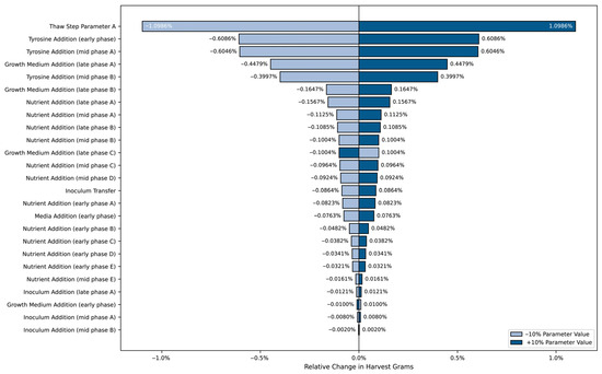
Figure 5.
Sensitivity analysis tornado chart showing the relative influence of a ±10% variation in key process inputs on HG. Parameter names were generalized by production phase to preserve proprietary process information.
As shown in Figure 5, certain parameters strongly affected yield fluctuations. The most impactful parameters were thaw media warming time, tyrosine addition weight at various stages, and nutrient addition volumes. Parameters with the largest bar lengths indicate a greater effect on HG when varied. Notably, an increase or decrease in thaw media warming time and tyrosine addition weight resulted in the highest sensitivity, highlighting the need for precise control to improve production yield.
4. Discussion
This study demonstrates the practical potential of data-driven methodologies for yield improvement in the upstream bioprocessing of mAbs. Using ML models trained on industrial batch data, we identified a subset of CPPs that consistently impacted HG, including nutrient addition timing, transfer windows, and biochemical markers such as glucose and lactate concentrations.
The ML models predicted values beyond historical averages, reinforcing the viability of data-driven decision-making in bioprocess environments. Importantly, these findings support earlier observations by Cheon et al. [27], who highlighted the ability of ML models to uncover nonlinear parameter dependencies and guide operational stability in complex bioprocesses. In our study, because the exploratory framework relied primarily on BFW predictions, the resulting parameter recommendations represent aggregate yield behavior and may not fully capture HT- or PCV-specific effects.
While ML models delivered actionable insights, their black-box nature limited interpretability and restricted the scope of model-based exploration. The RF, GBM, and SVR models frequently selected parameter values near predefined bounds, highlighting their tendency to overfit without embedded process constraints. This echoes the challenges identified by Helleckes et al. [14] and Cheng et al. [15], who cited ML model opacity as a barrier to implementation in GMP environments. The need to integrate expert knowledge and operational constraints into model-based analyses is critical to ensuring real-world applicability, particularly in highly regulated settings. A lack of specialized development environments and limited regulatory guidance further complicate efforts to scale ML implementations within manufacturing-grade bioprocess operations [8]. Furthermore, the models exhibited reduced performance for certain targets (e.g., HT and PCV), which aligns with the findings of Jones and Gerogiorgis [30], who emphasized the selective importance of variables across predictive tasks.
The sensitivity analysis helped identify high-impact variables, despite model opacity. By evaluating the effect of ± 10% changes in key parameters, the analysis guided the prioritization of process variables. This not only supports more focused control strategies but also reduces operational complexity by identifying parameters that can tolerate variation without compromising yield. These results reinforce the insights of Kaysfeld et al. [38], who showed that integrating dynamic control and scheduling analyses into mAb fed-batch operations could significantly enhance performance by manipulating nutrient profiles and timing. In both studies, model-guided analysis revealed that time-based process-input parameters were particularly influential, highlighting the importance of dynamic scheduling and phase-specific control in upstream processes.
Our findings add to the evidence supporting ML-driven yield improvement approaches in biologics production. The process insights derived from yield predictions align with prior work by Kornecki and Strube [5], who demonstrated that model-based upstream decision-making can reduce experimental burden and accelerate bioprocess development. Moreover, the hyperbox mixture regression approach proposed by Nik-Khorasani et al. [39] emphasizes the potential of interpretable, data-driven tools for evaluating parameter sensitivity and recommending practical adjustments. Their use of regression-based clustering complements the insights derived from our univariate models by offering an additional layer of interpretability and parameter segmentation. Together, these results strengthen the case for ML-assisted process control strategies that are not only predictive but also actionable in real-world production environments.
The following remarks summarize the key methodological uncertainties and limitations of the study. First, the model’s reliance on historical batch data—while practical—limits its capacity to capture process variability due to changing raw materials, bioreactor scale-up issues, and cell line evolution. Additionally, while the dataset contained 65 batches, the relatively low sample size limited generalizability and predictive accuracy for certain targets, particularly HT and PCV. This reflects broader challenges in biopharmaceutical ML adoption, as discussed by Singh and Singhal [23], including data fragmentation, low-frequency measurements, and inconsistent parameter recording.
To address these challenges, future work should incorporate hybrid models that blend mechanistic knowledge with data-driven learning—also highlighted by Rathore et al. [8] as a promising pathway for improving both interpretability and regulatory acceptance in bioprocess applications. Integrating real-time monitoring systems and PAT tools could enhance input resolution and provide more reliable decision-making under uncertainty. In addition, strategies such as simulation-based data augmentation or transfer learning may help overcome data scarcity in highly regulated environments. Furthermore, typical industry challenges, such as data silos, sparse sampling, and inconsistent record-keeping, continue to hinder widespread adoption of ML in biomanufacturing environments and must be addressed to fully leverage model-driven strategies. Exploring model generalizability across different mAb platforms or production scales would also help extend the impact of this approach.
Finally, although this study focused on offline, data-driven yield prediction, the proposed approach could support future integration into automated or supervisory control frameworks. In such settings, predictive models may serve as advisory or surrogate components that generate yield forecasts or recommend process adjustments based on real-time monitoring data. This conceptual linkage emphasizes how exploratory modeling outcomes, once validated, could inform control-oriented strategies for process adaptation and decision support.
5. Conclusions
This study highlights the practical potential of ML for yield improvement in the upstream bioprocessing of mAbs. By applying data-driven modeling and parameter-exploration techniques to historical production data, we achieved a predicted increase in harvested yield beyond previously recorded batch performance.
Despite this success, the analysis revealed key limitations of purely statistical approaches. The predictive models for HT and PCV showed limited reliability, emphasizing the need for further refinement or integration with mechanistic understanding. Moreover, the exploratory analysis often resulted in parameter values at the extreme ends of their allowable ranges—a behavior rooted in the black-box nature of the models and the absence of physical constraints or target ranges.
Future work should consider incorporating soft constraints or penalty functions to guide the exploratory data analysis toward realistic and controllable parameter values. Additionally, hybrid approaches that combine empirical modeling with mechanistic insights may offer more robust and interpretable solutions. Enhancing the prediction accuracy of HT and PCV, either through feature enrichment or model selection, remains an important area for continued investigation. In a broader context, the outcomes presented here may also inform future efforts to connect predictive modeling with process-control strategies, contributing to the gradual advancement toward data-driven and adaptive biomanufacturing.
Ultimately, this study provides a foundation for integrating ML into upstream process development, offering a pathway toward data-driven decision-making in biomanufacturing settings. However, success in scaling such approaches will depend not only on algorithmic performance but also on access to high-quality, structured process data. As highlighted in prior studies, the lack of standardized, readily accessible production data still limits broader ML adoption in bioprocessing. Addressing this through improved data infrastructure, contextual data integration, and possibly simulation-enhanced datasets will be essential to fully enable AI in industry.
Author Contributions
Conceptualization, B.R.S. and A.R.d.Q.; methodology, B.R.S. and A.R.d.Q.; software, B.R.S.; validation, B.R.S. and A.R.d.Q.; formal analysis, B.R.S. and A.R.d.Q.; investigation, B.R.S.; resources, B.R.S., A.R.d.Q. and L.H.; data curation, B.R.S.; writing—original draft preparation, B.R.S.; writing—review and editing, B.R.S., A.R.d.Q. and L.H.; visualization, B.R.S.; supervision, A.R.d.Q. and L.H.; project administration, B.R.S., A.R.d.Q. and L.H. All authors have read and agreed to the published version of the manuscript.
Funding
This research received no external funding.
Data Availability Statement
Due to confidentiality agreements and the sensitive nature of proprietary client information handled by the collaborating company, the data presented in this study are available upon request from the corresponding author.
Conflicts of Interest
The authors declare no conflicts of interest.
Abbreviations
The following abbreviations are used in this manuscript:
| BFW | Bioreactor final weight |
| CDMO | Contract development and manufacturing organization |
| CPPs | Critical process parameters |
| DL | Deep learning |
| EDA | Exploratory data analysis |
| GBM | Gradient boosting machine |
| GMP | Good Manufacturing Practice |
| HG | Harvested grams |
| HT | Harvest titer |
| mAb | Monoclonal antibody |
| MAE | Mean absolute error |
| ML | Machine learning |
| MSE | Mean squared error |
| PAT | Process analytical technologies |
| PCV | Packed cell volume |
| R2 | Coefficient of determination |
| RF | Random forest (regression) |
| SLSQP | Sequential least squares programming |
| SVR | Support vector regression |
References
- Ecker, D.M.; Jones, S.D.; Levine, H.L. The therapeutic monoclonal antibody market. mAbs 2015, 7, 9–14. [Google Scholar] [CrossRef]
- Walsh, G. Biopharmaceutical benchmarks 2018. Nat. Biotechnol. 2018, 36, 1136–1145. [Google Scholar] [CrossRef]
- Kelley, B. Industrialization of mAb production technology: The bioprocessing industry at a crossroads. mAbs 2009, 1, 443–452. [Google Scholar] [CrossRef]
- Mandenius, C.-F.; Brundin, A. Bioprocess optimization using design-of-experiments methodology. Biotechnol. Prog. 2008, 24, 1191–1203. [Google Scholar] [CrossRef] [PubMed]
- Kornecki, M.; Strube, J. Accelerating biologics manufacturing by upstream process modelling. Processes 2019, 7, 166. [Google Scholar] [CrossRef]
- Baako, T.-M.D.; Kulkarni, S.K.; McClendon, J.L.; Harcum, S.W.; Gilmore, J. Machine learning and deep learning strategies for Chinese hamster ovary cell bioprocess optimization. Fermentation 2024, 10, 234. [Google Scholar] [CrossRef]
- Khuat, T.T.; Bassett, R.; Otte, E.; Grevis-James, A.; Gabrys, B. Applications of machine learning in antibody discovery, process development, manufacturing and formulation: Current trends, challenges, and opportunities. Comput. Chem. Eng. 2024, 182, 108585. [Google Scholar] [CrossRef]
- Rathore, A.S.; Nikita, S.; Thakur, G.; Mishra, S. Artificial intelligence and machine learning applications in biopharmaceutical manufacturing. Trends Biotechnol. 2023, 41, 497–509. [Google Scholar] [CrossRef]
- Khanal, O.; Lenhoff, A.M. Developments and opportunities in continuous biopharmaceutical manufacturing. mAbs 2021, 13, 1903664. [Google Scholar] [CrossRef]
- Kornecki, M.; Schmidt, A.; Lohmann, L.; Huter, M.; Mestmäcker, F.; Klepzig, L.; Mouellef, M.; Zobel-Roos, S.; Strube, J. Accelerating biomanufacturing by modeling of continuous bioprocessing—Piloting case study of monoclonal antibody manufacturing. Processes 2019, 7, 495. [Google Scholar] [CrossRef]
- Guerra, A.C.; Glassey, J. Machine learning in biopharmaceutical manufacturing. Eur. Pharm. Rev. 2018, 23, 62–65. Available online: https://www.europeanpharmaceuticalreview.com/article/79130/machine-learning-bioprocessing/ (accessed on 8 April 2025).
- Mondal, P.P.; Galodha, A.; Verma, V.K.; Singh, V.; Show, P.L.; Awasthi, M.K.; Lall, B.; Anees, S.; Pollmann, K.; Jain, R. Review on machine learning-based bioprocess optimization, monitoring, and control systems. Bioresour. Technol. 2023, 370, 128523. [Google Scholar] [CrossRef]
- Duong-Trung, N.; Born, S.; Kim, J.W.; Schermeyer, M.-T.; Paulick, K.; Borisyak, M.; Cruz-Bournazou, M.N.; Werner, T.; Scholz, R.; Schmidt-Thieme, L.; et al. When bioprocess engineering meets machine learning: A survey from the perspective of automated bioprocess development. Biochem. Eng. J. 2023, 190, 108764. [Google Scholar] [CrossRef]
- Helleckes, L.M.; Hemmerich, J.; Wiechert, W.; von Lieres, E.; Grünberger, A. Machine learning in bioprocess development: From promise to practice. Trends Biotechnol. 2023, 41, 817–831. [Google Scholar] [CrossRef] [PubMed]
- Cheng, Y.; Bi, X.; Xu, Y.; Liu, Y.; Li, J.; Du, G.; Lv, X.; Liu, L. Artificial intelligence technologies in bioprocess: Opportunities and challenges. Bioresour. Technol. 2023, 369, 128451. [Google Scholar] [CrossRef]
- Farzan, P.; Mistry, B.; Ierapetritou, M.G. Review of the important challenges and opportunities related to modeling of mammalian cell bioreactors. Am. Inst. Chem. Eng. J. 2017, 63, 398–408. [Google Scholar] [CrossRef]
- Kyriakopoulos, S.; Ang, K.S.; Lakshmanan, M.; Huang, Z.; Yoon, S.; Gunawan, R.; Lee, D.-Y. Kinetic modeling of mammalian cell culture bioprocessing: The quest to advance biomanufacturing. Biotechnol. J. 2018, 13, 1700229. [Google Scholar] [CrossRef] [PubMed]
- Rish, A.J.; Huang, Z.; Siddiquee, K.; Xu, J.; Anderson, C.A.; Borys, M.C.; Khetan, A. Identification of cell culture factors influencing afucosylation levels in monoclonal antibodies by partial least-squares regression and variable importance metrics. Processes 2023, 11, 223. [Google Scholar] [CrossRef]
- Bayer, B.; Duerkop, M.; Pörtner, R.; Möller, J. Comparison of mechanistic and hybrid modeling approaches for characterization of a CHO cultivation process: Requirements, pitfalls and solution paths. Biotechnol. J. 2023, 18, 2200381. [Google Scholar] [CrossRef]
- Procopio, A.; Cesarelli, G.; Donisi, L.; Merola, A.; Amato, F.; Cosentino, C. Combined mechanistic modeling and machine-learning approaches in systems biology—A systematic literature review. Comput. Methods Programs Biomed. 2023, 240, 107681. [Google Scholar] [CrossRef]
- Schweidtmann, A.M.; Zhang, D.; von Stosch, M. A review and perspective on hybrid modeling methodologies. Digit. Chem. Eng. 2024, 10, 100136. [Google Scholar] [CrossRef]
- Chen, Y.; Yang, O.; Sampat, C.; Bhalode, P.; Ramachandran, R.; Ierapetritou, M. Digital twins in pharmaceutical and biopharmaceutical manufacturing: A literature review. Processes 2020, 8, 1088. [Google Scholar] [CrossRef]
- Singh, A.; Singhal, B. Role of machine learning in bioprocess engineering: Current perspectives and future directions. In Design and Applications of Nature Inspired Optimization; Singh, D., Garg, V., Deep, K., Eds.; Springer: Cham, Switzerland, 2022; pp. 39–54. [Google Scholar] [CrossRef]
- von Stosch, M.; Oliveira, R.; Peres, J.; Feyo de Azevedo, S. Hybrid semi-parametric modeling in process systems engineering: Past, present and future. Comput. Chem. Eng. 2014, 60, 86–101. [Google Scholar] [CrossRef]
- Goodfellow, I.; Bengio, Y.; Courville, A. Deep Learning; MIT Press: Cambridge, MA, USA, 2016; Available online: http://www.deeplearningbook.org (accessed on 8 April 2025).
- Géron, A. Hands-On Machine Learning with Scikit-Learn, Keras & TensorFlow: Concepts, Tools, and Techniques to Build Intelligent Systems, 3rd ed.; O’Reilly Media: Sebastopol, CA, USA, 2022. [Google Scholar]
- Cheon, A.; Sung, J.; Jun, H.; Jang, H.; Kim, M.; Park, J. Application of various machine learning models for process stability of bio-electrochemical anaerobic digestion. Processes 2022, 10, 158. [Google Scholar] [CrossRef]
- Hastie, T.; Tibshirani, R.; Friedman, J. The Elements of Statistical Learning: Data Mining, Inference, and Prediction, 2nd ed.; Springer: New York, NY, USA, 2009. [Google Scholar] [CrossRef]
- Breiman, L. Random forests. Mach. Learn. 2001, 45, 5–32. [Google Scholar] [CrossRef]
- Jones, W.; Gerogiorgis, D.I. Dynamic optimisation of fed-batch bioreactors for mAbs: Sensitivity analysis of feed nutrient manipulation profiles. Processes 2023, 11, 3065. [Google Scholar] [CrossRef]
- Pedregosa, F.; Varoquaux, G.; Gramfort, A.; Michel, V.; Thirion, B.; Grisel, O.; Blondel, M.; Prettenhofer, P.; Weiss, R.; Dubourg, V.; et al. Scikit-learn: Machine learning in Python. J. Mach. Learn. Res. 2011, 12, 2825–2830. [Google Scholar]
- Friedman, J.H. Greedy function approximation: A gradient boosting machine. Ann. Stat. 2001, 29, 1189–1232. [Google Scholar] [CrossRef]
- Drucker, H.; Burges, C.J.C.; Kaufman, L.; Smola, A.; Vapnik, V. Support vector regression machines. Adv. Neural Inf. Process. Syst. 1997, 9, 155–161. [Google Scholar]
- Chai, T.; Draxler, R.R. Root mean square error (RMSE) or mean absolute error (MAE)?—Arguments against avoiding RMSE in the literature. Geosci. Model Dev. 2014, 7, 1247–1250. [Google Scholar] [CrossRef]
- Kraft, D. A Software Package for Sequential Quadratic Programming; Technical Report DFVLR-FB 88–28; DLR German Aerospace Center—Institute for Flight Mechanics: Cologne, Germany, 1988; Available online: http://degenerateconic.com/uploads/2018/03/DFVLR_FB_88_28.pdf (accessed on 16 September 2025).
- Molnar, C. Interpretable Machine Learning: A Guide for Making Black Box Models Explainable; Leanpub: Victoria, BC, Canada, 2019; Available online: https://christophm.github.io/interpretable-ml-book/ (accessed on 12 April 2025).
- Saltelli, A.; Ratto, M.; Andres, T.; Campolongo, F.; Cariboni, J.; Gatelli, D.; Saisana, M.; Tarantola, S. Global Sensitivity Analysis: The Primer; John Wiley & Sons: Chichester, UK, 2008. [Google Scholar] [CrossRef]
- Kaysfeld, M.W.; Kumar, D.; Nielsen, M.K.; Jørgensen, J.B. Dynamic optimization for monoclonal antibody production. IFAC Pap. Online 2023, 56, 6229–6234. [Google Scholar] [CrossRef]
- Nik-Khorasani, A.; Khuat, T.T.; Gabrys, B. Hyperbox mixture regression for process performance prediction in antibody production. Digit. Chem. Eng. 2025, 14, 100221. [Google Scholar] [CrossRef]


Disclaimer/Publisher’s Note: The statements, opinions and data contained in all publications are solely those of the individual author(s) and contributor(s) and not of MDPI and/or the editor(s). MDPI and/or the editor(s) disclaim responsibility for any injury to people or property resulting from any ideas, methods, instructions or products referred to in the content. |
© 2025 by the authors. Licensee MDPI, Basel, Switzerland. This article is an open access article distributed under the terms and conditions of the Creative Commons Attribution (CC BY) license (https://creativecommons.org/licenses/by/4.0/).