Abstract
With the rapid development of distributed energy and electric vehicles (EVs), the limited hosting capacity of distribution networks has severely impacted their economic dispatch and safe operation. To address these challenges, in this work, an optimal planning model considering the uncertainty of wind and solar power output is proposed, aiming to determine the location and capacity of electric vehicle charging stations (EVCSs). The model seeks to minimize the total costs, voltage fluctuations, and network losses, subject to constraints such as EV user satisfaction and grid company satisfaction. A multi-objective heat exchange optimization algorithm under Gaussian mutation (MOTEO-GM) is employed to validate the model on an extended IEEE-33 bus system and a real-world case in the University Town area of Chenggong District, Kunming City. Simulation results indicate that, in the test system, voltage fluctuations and system power losses are decreased by 43.05% and 37.47%, respectively, significantly enhancing the economic operation of the distribution grid.
1. Introduction
As environmental sustainability and energy shortages become increasingly pressing issues, new energy technologies have experienced rapid development. A large number of distribution generations (DGs) have been integrated into the power grid, which has not only increased the structural complexity of power systems but also turned site selection and capacity planning into a challenging problem. Conventional loads are easily influenced by human behavior, exhibiting temporal variability and randomness. Wind power and photovoltaic distributed power sources, whose output is affected by wind speed and sunlight intensity, also exhibit strong uncertainty and seasonality. Neglecting these characteristics can severely compromise the accuracy of distribution grid planning. With continuous technological progress and government promotion of electric vehicles (EVs), the penetration of EVs into the load profile has been increasing annually, exerting an irreversible influence on distribution networks. Therefore, a rational solution is urgently required to respond to this emerging challenge. EV charging loads are also influenced by human habits and exhibit temporal characteristics, which has led to growing interest in the optimal planning of electric vehicle charging stations (EVCSs).
In recent years, many domestic and international scholars have conducted extensive research on the site selection and capacity optimization of EVCS. Ref. [1] proposed a three-tier framework to enhance EVCS flexibility through distribution network design and developed incentive mechanisms for EVCSs within coupled power and transportation networks. These mechanisms aim to achieve dynamic equilibrium by maximizing profits and ensuring operational safety. That study only considered grid satisfaction conditions, such as construction costs, voltage fluctuations, and network losses, during periods of low renewable energy output; the charging loads for systems A and B were reduced by 11.01 MW and 7.88 MW, respectively, effectively improving grid satisfaction. However, this does not deeply consider user satisfaction. Ref. [2] introduced a novel strategy for determining the optimal location of EVCSs, greatly helping the EV and distribution industries improve system reliability and efficiency; active power losses decreased by 78.4% year-on-year, total voltage deviation decreased by 86.1% year-on-year, and total operating costs were optimized by 78.4%, effectively meeting grid satisfaction requirements. However, this still only considers grid satisfaction and does not consider user satisfaction. Ref. [3] optimized and evaluated photovoltaic–wind–battery/EV charging station systems, primarily aiming to minimize total net present value costs and power supply interruption probability. When load, irradiance, and wind speed each increase by 30%, costs increase by 1.63%, 0.48%, and 0.60%, respectively. Similarly, the study considers grid satisfaction metrics like grid costs and power outage probability, yet it neglects user satisfaction. This one-sided focus on grid satisfaction without considering user satisfaction can lead to numerous issues. Ref. [4] proposed a novel planning framework to determine the optimal location, capacity, and type of electric vehicle charging stations within multi-energy systems. Comprehensive planning for all energy resources achieves cost savings by addressing cost issues, including both user satisfaction and grid satisfaction. In Cases 3 and 4, compared to Case 1, line losses decreased by 15% due to V2G injecting active power into the grid, effectively enhancing grid user satisfaction. However, that study solely focuses on grid satisfaction costs without considering safety dimensions like voltage fluctuations and network losses. This research overly prioritizes cost reduction at the expense of safety, representing a flawed and undesirable approach. Ref. [5] found that increasing EV utilization requires fast-charging systems, which may overload the grid and necessitate costly additional installations and equipment. To address this, Ref. [5] focused on grid satisfaction without examining user satisfaction. This research is clearly too narrow and should incorporate user satisfaction considerations. Both Refs. [6,7] addressed uncertainty analysis for wind and solar power, but neither conducted in-depth uncertainty studies on their output. In Ref. [6], voltage fluctuations and system network losses decreased by 36.73% and 35.41%, respectively, effectively enhancing the stability and economic efficiency of the distribution network. However, Ref. [7] aimed to maximize technical, financial, and social benefits while considering grid satisfaction. When distributed generation and distribution static compensators are deployed concurrently, voltage distribution is significantly improved, with power losses reduced by 36% and 40% in the 33-node and 108-node systems, respectively. Although investment costs increase, energy loss costs and emission costs are substantially reduced. Energy loss costs and emission costs decrease by 35% and 27% in the 33-node system, and by 15% and 20% in the 108-node system, yet because it makes no mention of user satisfaction, this research is clearly incomplete.
First, this work comprehensively considers the uncertainty of wind turbine and photovoltaic output caused by environmental variability, as well as the volatility of demand loads. Wind speed, solar irradiance, and load demand are modeled in a time-series framework. Second, based on Monte Carlo random simulation, a time-series model of EV charging load is established and combined with a wind–solar–load model to generate multi-dimensional distributed power source planning scenarios [8,9,10,11]. Refs. [8,9,10,11] do not discuss wind and solar uncertainty. It is only mentioned in passing, and no specific research has been conducted. This study fills the gap in research on wind and solar uncertainty. To improve computational efficiency, clustering algorithms such as fuzzy kernel clustering are used to cluster complex multi-dimensional scenarios, yielding representative, typical operational scenarios. Then, an optimal EVCS planning model is formulated based on the coupled wind–solar–load system, with objectives including the minimization of total construction cost, user waiting time, voltage deviation, and network losses. The model comprehensively considers the interests of three key stakeholders, namely, investors, EV users, and grid operators, to achieve a balanced, win–win planning outcome [12,13,14,15,16,17,18]. In Refs. [12,13,14,15,16,17,18], user satisfaction and grid satisfaction were only considered individually, without comprehensively balancing the relationship between the two. Therefore, this study is able to reflect the relationship between the interests of the two parties.
Currently, the optimal planning for EVCSs remains primarily focused on construction costs and user satisfaction, with most studies considering only basic load forecasts limited to EV demand. Research on the uncertainty of wind and solar power under high penetration rates and the impact of EVCSs on distribution grids is still at an early stage. To address this issue, this paper couples wind and solar power generation output models with EV load, thereby establishing a three-level planning framework that integrates the wind, solar, and load dimensions. Based on the aforementioned model, an optimal planning method for EVCS is proposed that accounts for the uncertainty of wind and solar power generation, as well as EV load.
Finally, the opposition-based particle swarm optimization with multi-objective heat exchange optimization algorithm under Gaussian mutation (MOTEO-GM) is applied to the extended IEEE-33 node system to validate the model’s effectiveness. Subsequently, the entire planning framework is implemented in a real-world case study involving EVCS deployment at the University Town of Chenggong District, Kunming City. Its performance is compared with other optimization algorithms, including the multi-objective artificial lemming algorithm (MOALA), the multi-objective hawkfish optimization algorithm (MOHFOA), the multi-objective mayfly algorithm (MOMA), multi-objective particle swarm optimization (MOPSO), and the non-dominated sorting genetic algorithm III (NSGA-III). The results demonstrate the superior effectiveness of the proposed EVCS siting and planning model in accounting for wind and solar uncertainty, as well as the high applicability of the MOTEO-GM algorithm to EVCS planning problems.
The remainder of this paper is structured as follows:
Section 2 introduces the wind and solar power output models and the electric vehicle load model, and combines them. Section 3 introduces a planning model for electric vehicle charging stations with voltage fluctuations and network losses as objective functions; Section 4 describes the main algorithm of this paper, based on a multi-objective heat exchange algorithm model under Gaussian mutation; Section 5 validates the above model using an extended IEEE-33 node network and applies it to an actual case study in a district of Kunming City, Yunnan Province, demonstrating the effectiveness of the algorithm.
2. Uncertainty of Wind Power Output and Establishment of Electric Vehicle Load Models
2.1. Overall Framework
The overall framework of this study is shown in Figure 1 [6]. It mainly includes three parts: (1) the establishment of wind and solar power output and EV load models; (2) the optimal planning of an EVCS; (3) the solution to multi-objective models.
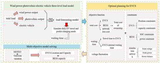
Figure 1.
Overall framework diagram.
2.2. Consideration of Scenarios with Uncertain Wind and Solar Power Output
2.2.1. Wind Power Output Model
The wind power output model is closely related to the magnitude of natural wind speed. At the same time, the location of wind farms and wind fields is also closely related to the establishment of wind farms. Based on existing research, a two-parameter Weibull distribution can be used to simulate changes in wind speed, whose probability density function is expressed as follows [19]:
where represents the wind speed at the wind turbine at location at time ; is the shape parameter of the wind turbine at location at time ; and denotes the scale parameter of the wind turbine at location at time . The specific distribution diagram is shown in Figure 2.

Figure 2.
Probability density function of the two-parameter Weibull distribution.
In this work, considering that wind power is controlled at constant power, the relationship between wind power output and wind speed at a given location can be approximately represented by the following function:
where represents the rated capacity of the representative office’s wind farm. , , and are the cut-in wind speed, rated wind speed, and cut-out wind speed, respectively.
2.2.2. Photovoltaic Power Output Model
The variability of photovoltaic power output is influenced by multiple factors, including environmental conditions, geographical location, and material properties. Different environmental conditions result in varying levels of solar radiation, and different geographical locations experience significant differences in sunlight duration. Moreover, photovoltaic panels made from different materials or based on different technologies can generate different levels of electricity under identical irradiation conditions. However, in this work, only the primary factor that affects photovoltaic power output is considered, i.e., the variation in sunlight intensity throughout the day. Typically, the beta distribution is employed to describe the variation in sunlight intensity over a 24 h period. The specific expression is as follows [20,21,22]:
where and represent the light intensity at position and its maximum value; Similarly, and denote the two parameters of the beta distribution at position and time, respectively. The specific distribution diagram is shown in Figure 3.
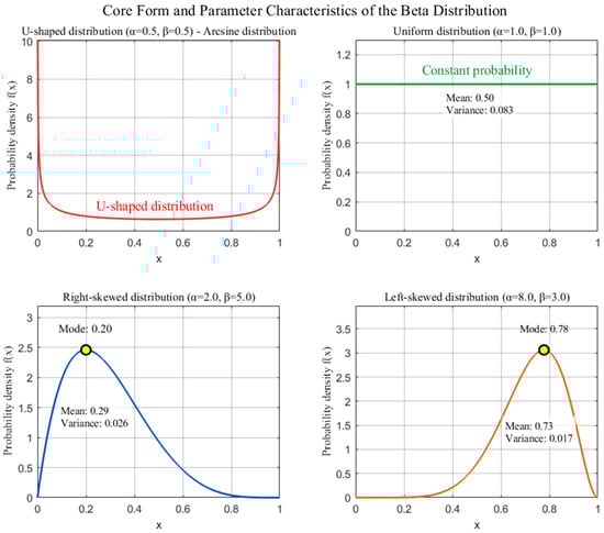
Figure 3.
Beta distribution probability density function graph.
The expression for photovoltaic output is
where represents the rated output of the photovoltaic panel at the representative office; and denote the actual and test conditions of the photovoltaic module at the representative office, respectively; is the light irradiation point at the representative office.
2.3. Electric Vehicle Load Model
2.3.1. EV Daily Mileage Distribution Function and Distribution Chart
The daily mileage follows a log-normal distribution, , whose probability density function is described by
where represents the daily mileage, with units of minutes; and denote the mean and standard deviation of the daily mileage; and = 3.3 and = 0.88 [6]. The daily mileage probability distribution chart for EVs can be obtained from Equation (5), as shown in Figure 4 [6].

Figure 4.
Probability diagram of daily mileage.
2.3.2. EV Initial Driving Distribution Function and Its Distribution Chart
The distribution of EV departure times is easily influenced by factors such as travel plans, holidays, morning and evening rush hours, and weather changes. To simplify the model and ensure its rationality, this study excludes the impact of such sudden or irregular events and instead focuses solely on regular daily travel patterns [23,24]. The departure behavior of EVs, which aligns with typical daily commuting patterns, can be modeled using a bimodal distribution function, whose probability density function is defined as follows:
where t represents travel time in minutes; , and , denote the mean and standard deviation of the first and second peaks, respectively. The values of these parameters in this work are = 8, = 3, = 18, and = 2.25 [6].
2.4. EV Initial Charge State
State of charge (SOC) has a significant impact on both user charging time and the charging demand of EVs. Therefore, this study incorporates the effect of SOC into the planning model. Since SOC values are inherently variable and not fixed, SOC is modeled as a random variable. Its probability density function is given as follows:
where is the initial SOC of the EV, and denotes the average SOC, and is the standard deviation of SOC. The values of and are set as 0.3 and 0.15, respectively [6].
2.5. User Waiting Time Model
EV users arriving at a charging station must queue on a first-come, first-served basis. If no charging pile is available upon arrival, the vehicle must enter a waiting queue for charging [25].
The EV user waiting time is calculated by
where represents the time when the EV arrives at the nearest EVCS, and denotes the time required to complete charging at a charging pile within the station.
2.6. Method for Constructing Typical Scenarios
Based on the probability density functions representing the uncertainty of wind and solar power output, as well as the EV load forecasting model described above, this study applies fuzzy kernel clustering to data collected from a district in Kunming to divide the year into four representative scenarios: spring, summer, autumn, and winter. Each scenario reflects distinct wind and solar power generation characteristics. The detailed scenario generation process is as follows [26,27]:
(1) Collect historical wind and solar power output data and EV charging demand data from a specific district in Kunming City; then, perform data cleaning and normalization.
(2) Select a specific Kernel-Based Fuzzy C-Means Clustering (KFCM) method.
(3) Define representative scenarios based on output characteristics, labeling the four clusters as spring, summer, autumn, and winter scenarios.
(4) Use the four seasonal scenarios and the aforementioned solar and wind power output profiles for subsequent load model establishment.
KFCM is an improvement and extension of the traditional Fuzzy C-Means (FCM) algorithm. Its core mechanism involves mapping linearly inseparable data from the original low-dimensional space to a high-dimensional feature space via kernel functions, thereby enabling linearly separable clustering in the high-dimensional domain. This addresses the limitations of traditional FCM, which struggles with clustering nonlinear data and is susceptible to noise interference. Essentially, it employs the “Kernel Trick” to circumvent direct computations in high dimensions while preserving the flexible partitioning characteristics of fuzzy clustering.
The clustering principle of the KFCM algorithm in the feature space is intended to minimize the sum of the weighted squared distances between samples and cluster centers, which is described as follows:
where is a constant; and represent the number of clusters and the number of samples, respectively; is the th sample; is the center of the th cluster; is the membership function of the th sample in the th cluster, meeting and ; and is the membership matrix, .
Expanding Equation (9), we obtain
We define the kernel function, , and perform the kernel substitution; then,
Substituting Equation (10) into Equation (9), we obtain
where if is the Gaussian kernel function, then .
From Equation (11), it can be concluded that still belongs to the input space, but KFCM introduces weighted coefficients to the cluster centers, thereby giving reasonable weight values to noise points and outliers.
In this study, we employed a Windows 11 Professional 64-bit operating system with an Intel® CoreTM i5-14600K processor (3.50 GHz) running on an x64 architecture. The manufacturer is Intel, and the city and location of purchase are Shanghai, China. Solutions were computed using MATLAB R2024b. The resulting output profiles for each scenario are shown in Figure 5. The steps of clustering are detailed in Table A1 of Appendix B, and the clustering results are presented in Table A2 of Appendix B.
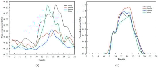
Figure 5.
Output diagrams for four typical scenarios. (a) Wind power output diagram. (b) Photovoltaic output diagram.
3. EVCS Site Selection and Capacity Planning Optimization Model
3.1. Objective Function
3.1.1. EVCS Investment and Construction Costs
This work considers the investment and construction costs of EVCS in the planning process. To achieve more cost-effective site selection and capacity planning, it is essential to account for the comprehensive cost structure [28,29,30].
The comprehensive costs of EVCS combined with a battery energy storage system (BESS) are as follows:
where represents the total cost of the EVCS and BESS system, i.e., the overall construction cost of the charging station; denotes the annualized total cost of the EVCS investment and construction; is the full life cycle cost of the BESS investment and construction; represents the cost of power loss.
where represents the average discount rate; denotes the operating period; means the number of EVCS; and , , and represent the land purchase cost, construction cost, and operating and maintenance costs, respectively.
where represents the unit land price in different regions. The regions are classified based on land use characteristics, and the corresponding guideline prices vary accordingly. These prices are affected by factors such as proximity to the city center and the post-development land use type, making this value variable. represents the number of charging stations within the ith charging station; represents the ratio coefficient of the parking space area after the conversion of the building and other areas; and denote the parking space area and the equipment area, respectively.
where represents the fixed cost of the charging station; means the purchase cost; denotes the capacity; and represents the investment coefficient related to capacity.
where represents the operation and maintenance coefficient related to charging station capacity.
where represents the service life of the BESS; denotes the number of BESS units; is the BESS discount rate; , , , and mean the total investment cost, operational and maintenance cost, replacement cost, and disposal and recycling cost, respectively.
where and represent the costs of the storage battery and inverter.
where and denote the ratio of OP to battery investment costs and the proportion of inverter investment costs, respectively.
where represents the number of times the BESS is replaced; is the replacement cycle of the BESS; and represents the annual reduction rate of the BESS cost.
where is the recovery coefficient of the battery and inverter.
where is the conversion coefficient between power loss and loss cost; and denote the active power loss in the distribution network before connecting to the charging station and BESS and the active power loss after connecting to the charging station and BESS, respectively.
3.1.2. Waiting Time Costs
When EV users arrive at a charging station, if no charging piles are available, they must wait in a queue according to the first-come, first-served principle. Users who arrive earlier will begin charging earlier. Later-arriving EV users incur a waiting time equal to the sum of the previous user’s charging time and waiting time. During this period, users experience waiting-related costs, referred to as user waiting time costs. These costs consist of both the time spent traveling to the charging station and the time spent waiting in line and can be calculated as follows [31,32,33]:
where represents the number of EVs; denotes the shortest distance from the ith vehicle to the jth EVCS; is the average driving speed; and signifies the waiting time of the ith vehicle at the jth EVCS.
3.1.3. Voltage Fluctuations
The constraints for voltage fluctuations are as follows:
where represents the number of nodes; represents time; denotes the voltage of the node i at time j; and represents the average voltage of node during the period [1–T].
3.2. Constraints
3.2.1. Charging Station Distance Constraints
In order to prevent EVCSs from being built too far apart or too close together, which would reduce user satisfaction in the former case and lead to a waste of resources in the latter, it is necessary to impose a distance constraint:
where represents the charging radius of the charging station, and denotes the distance between two charging stations.
3.2.2. Charging Station Capacity Constraints
The constraints for charging stations are as follows:
where is the maximum charging demand in this area, and represents the maximum service time of the charging station.
3.2.3. Node Voltage Constraints
The constraints for voltage nodes are as follows:
where and represent the voltage threshold after the node is connected to the EVCS.
where and represent the active and reactive power injected by the node; represents the total active power loss of the system; denotes the total reactive power loss of the system; and are the active and reactive loads of the node; and and are the active and reactive power output of the node, n, after connecting to the EVCS.
3.2.4. SOC Constraints for BESS
The charging and discharging of energy storage systems occur within a specific power range.
where represents the SOC of BESS.
3.2.5. BESS Charging and Discharging Power Constraints
The constraints are as follows:
where and represent the rated power of the BESS.
4. Model Solving Based on MOTEO-GM
4.1. MOTEO Algorithm
Thermal exchange optimization (TEO) is a novel optimization algorithm based on Newton’s cooling law, characterized by fast convergence and strong optimization capabilities. MOTEO extends the TEO algorithm to the field of multi-objective optimization. Its core challenge lies in the fact that the solution to a multi-objective problem is no longer a single scalar value but rather a set of Pareto optimal solutions. Therefore, MOTEO requires introducing multi-objective processing strategies on top of the original TEO mechanism. While retaining TEO’s physical update mechanism, the MOTEO algorithm shifts its core comparison criterion from “scalar value comparison” to “Pareto dominance comparison.” It also incorporates external archiving and a diversity maintenance mechanism based on crowding distance. The transition from TEO to MOTEO fundamentally represents a paradigm shift from scalar optimization to vector optimization. MOTEO performs well in solving multi-objective problems, delivering a series of balanced trade-off solutions. However, its efficiency typically falls below TEO due to additional computational overhead (domination checks, archive maintenance). The MOTEO algorithm introduces a thermally meaningful energy exchange mechanism, where its energy transfer model effectively guides particles toward the Pareto front, achieving fast convergence. By combining Pareto dominance and diversity preservation strategies, it can simultaneously optimize multiple conflicting objectives and obtain a uniformly distributed set of non-inferior solutions. However, the standard MOTEO algorithm still exhibits certain deficiencies. Therefore, this work introduces several enhancement mechanisms, such as Gaussian mutation, crowded distance, and roulette wheel selection, to improve its overall performance. These mechanisms enhance the performance of the standard MOTEO algorithm from three key perspectives: local search or perturbation, solution set distribution control, and parent selection strategy. This enables the algorithm to obtain high-quality solution sets that are closer to the true Pareto frontier, more uniformly distributed, and have a broader range when solving complex multi-objective optimization problems. The initial population size in this algorithm is 300, with the fitness function minimizing construction costs, voltage fluctuations, and network losses. The specific solution process is illustrated in Figure 6 [34]. To prove the effectiveness of the added mechanism, this paper conducted tests on the mechanism’s analytical functions and instance test functions. For details, please refer to Figure A1, Figure A2, Figure A3, Figure A4, Figure A5, Figure A6, Figure A7, Figure A8, Figure A9 and Figure A10 in Appendix A.
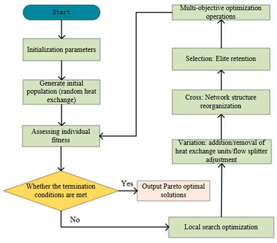
Figure 6.
MOTEO algorithm flowchart.
4.2. Solving the Model Based on Gaussian Mutation
Gaussian mutation is a commonly used perturbation strategy in evolutionary algorithms such as genetic algorithms and particle swarm optimization. It is typically employed to perform local fine-grained searches in the solution space or to escape local optima. Gaussian mutation generates new solutions by adding a random perturbation that follows a normal distribution to the current solution, as follows:
where represents a Gaussian random function with a mean of 0 and a variance of , in which controls the variation intensity and typically decreases with each iteration.
The crowding distance measures an individual’s sparsity on the Pareto front. The larger the value, the more isolated the individual is, and the more it should be prioritized for retention. After sorting each objective function, m, in ascending order, the crowding distance for each individual is calculated as follows:
where and represent the adjacent target values, and and denote the maximum and minimum target values, respectively.
The total congestion distance is expressed as
Roulette wheel selection is used to determine the selection probability of individuals based on their crowding distance. Individuals with larger crowding distances—i.e., those located in sparser regions of the solution space—are assigned higher probabilities of being selected as leaders.
Probability calculation:
Cumulative probability:
Crowding distance quantifies sparsity, and roulette-based selection of leaders based on sparsity jointly maintains the uniformity and diversity of the Pareto frontier.
The solution procedure of the MOTEO-GM-based joint sitting and sizing model for electric vehicle charging stations integrated with BESS is illustrated in Figure 7.
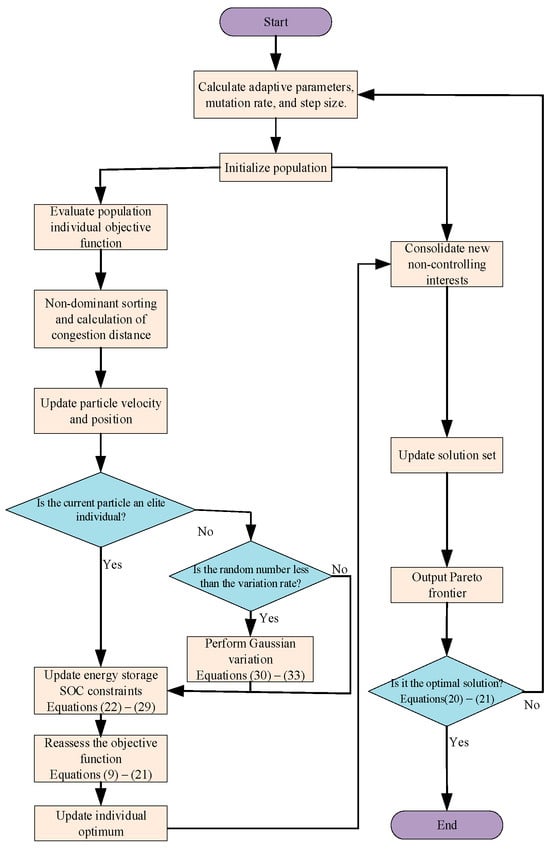
Figure 7.
Flowchart of the solution process for the MOTEO-GM electric vehicle charging station and BESS joint site selection and capacity determination model.
5. Case Study
Kunming, the provincial capital of Yunnan Province in China, is located between 102°10′ and 103°40′ east longitude and 24°23′ and 26°33′ north latitude. As of 2024, it has a permanent population of 8.687 million and serves as an important gateway for China’s opening-up to South Asia and Southeast Asia, as well as a front-line hub for the Belt and Road Initiative. In this work, the University Town in Chenggong District, Kunming City, Yunnan Province, will be used as a practical case study. Figure 8, below, shows the specific location of the University Town in Kunming City. It is noted that the simulation results are limited to an actual case study.
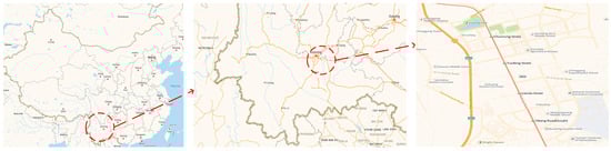
Figure 8.
Map of Chenggong District in Kunming.
5.1. Test Model
First, prior to conducting the model testing, we make the following declarations regarding the model parameters: (1) the number of electric vehicles is set at 2000; (2) both the EV and EVCS considered are of the BYD series; (3) the BESS is installed within the EVCS, so the installation locations of the BESS and EVCS are the same; (4) the charging station operates in fast-charging mode.
To verify the effectiveness of the proposed model, preliminary testing is conducted on the expanded IEEE-33 bus system. Wind power generation units with a capacity of 0.45 MW are installed in buses 21 and 24, while photovoltaic generation units with a capacity of 1.5 MW are configured in buses 17 and 31. The specific configuration diagram is shown in Figure 9 [6]. The numbers 1 to 33 in the Figure 9 respectively represent 33 nodes.
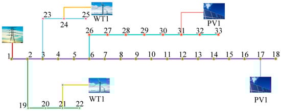
Figure 9.
Extended IEEE-33 node diagram.
Before conducting model testing, this study provides detailed descriptions of the model structure and system parameters, as shown in Table 1, Table 2 and Table 3.

Table 1.
System parameters.
Table 2.
Comparison of algorithm parameters.
Table 3.
Basic parameters of EV [6].
Based on the establishment of the above model and the setting of model parameters, the simulation results obtained using the IEEE-33 bus system are shown in Table 4. From the results, it can be observed that the total cost of the MOTEO-GM-based planning scheme for electric vehicle charging stations is CNY 5,454,110, which is 13.64% higher than the lowest-cost solution provided by the MOPSO algorithm (CNY 4,749,100). Although the cost of MOTEO-GM is slightly inferior to other algorithms in this study, the cost in the power grid is less important than voltage fluctuations and network losses that affect the safe operation and economic dispatch of the power system network. MOTEO-GM achieves significant improvements in both voltage fluctuations and network losses compared to other algorithms. Specifically, network losses are reduced by 37.47%, 13.02%, 3.44%, 4.60%, and 0.52% compared to MOALA, MOHFOA, MOPSO, MOMA, and NSGA-III, respectively. Similarly, voltage fluctuations are reduced by 43.05%, 21.57%, 13.43%, 8.13%, and 6.24% compared to MOALA, MOHFOA, MOPSO, MOMA, and NSGA-III, respectively. Based on the above analysis, MOTEO-GM demonstrates certain advantages and strong applicability in this model.
Table 4.
IEEE-33 node simulation test results.
In Figure 10, the voltage fluctuations of each algorithm are respectively presented. It can be concluded that the voltage fluctuation of MOTEO-GM is the smallest, which proves the effectiveness of MOTEO-GM in this paper.

Figure 10.
Voltage fluctuations of each algorithm under the IEEE-33 test node extension.
Table 5 shows the locations, capacities, and numbers of charging stations accommodated by six EVCS under various optimization algorithms.
Table 5.
EVCS capacity configuration table under IEEE-33 node.
Furthermore, to demonstrate that incorporating Gaussian mutation and roulette wheel selection into this study can significantly improve the algorithm’s shortcomings, this paper selected mu—the most critical parameter in Gaussian mutation—as the variable. Sensitivity analysis was conducted using cost as the observed value, with the results shown in Figure 11.
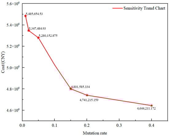
Figure 11.
Sensitivity curve analysis chart.
5.2. Planning of the Actual Area
To further validate the effectiveness and practical applicability of the proposed model, it is applied to the University Town in Chenggong District, Kunming City, Yunnan Province, to conduct optimal planning for EVCSs in the area, based on the aforementioned test model. To demonstrate the impact of EV charging on the power grid, and since obtaining actual grid topology data is unfeasible, this paper assumes each region constitutes a grid node [35]. The specific system parameters can be found in Table A3 of Appendix B. An improved 69-node grid model was re-established for simulation testing. This method has been thoroughly validated in domestic research, as detailed in Ref. [6]. The corresponding distribution network structure is shown in Figure 12 [6].

Figure 12.
Diagram of road network conversion structure.
It shows a transformation of the road area into a distribution network node structure in the Figure 12. Eventually, an actual case test was conducted using the improved 69-node model.
This section first predicts the traffic flow in the region, incorporates the predicted traffic flow into the charging demand calculation model, and derives the charging demand distribution across each time segment of the day, as shown in Figure 13.
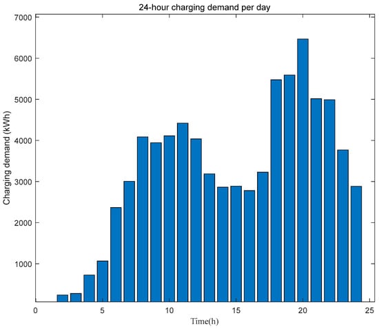
Figure 13.
Charging demand within a day.
Based on the aforementioned model, following the simulation process, the graph of the IEEE-33 bus system is transformed into the road network topology structure shown in Figure 9. Similarly, different wind and solar generation systems with varying outputs are connected to different nodes to construct a planning diagram that closely aligns with real-life scenarios. Similar to the IEEE-33 bus system, 0.45 MW wind power generation systems are configured at nodes 16 and 67, and 1.5 MW photovoltaic power generation systems are configured at nodes 56 and 33. The planning result diagram is shown in Figure 14.
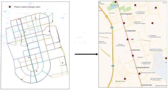
Figure 14.
EVCS planning diagram.
The charging and discharging power and SOC changes in the BESS at each charging station under the MOTEO optimization results are illustrated in Figure 13.
Figure 15 shows the charging and discharging power and SOC changes of each BESS within a day. It can be seen that all 10 BESS units operate continuously throughout the day, with their SOC levels maintained between 20% and 90%, which is beneficial for ensuring both the operational lifespan and safety of the BESS units.
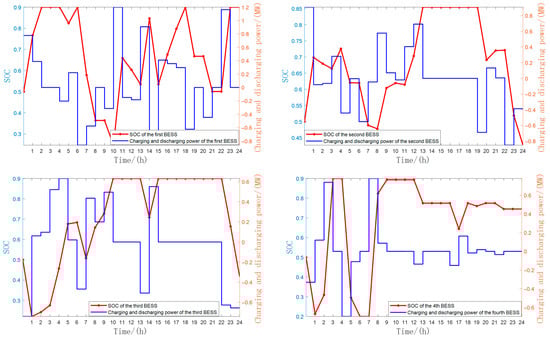
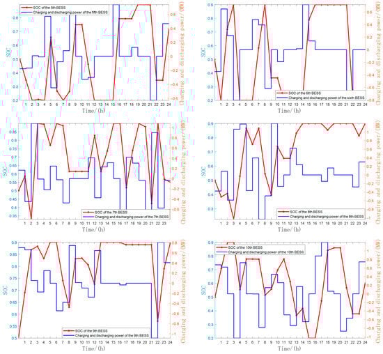
Figure 15.
Changes in charging and discharging power and SOC for each BESS.
6. Conclusions
This study first establishes an uncertainty model for wind and solar power output and then applies the Monte Carlo method to predict traffic flow in the University Town of Chenggong District, Kunming City, while simulating the corresponding EV charging demand. Finally, wind and solar power outputs are integrated with EV loads. This study aims to maximize the satisfaction of three stakeholders, i.e., EVCS developers, EV users, and power grid companies, by establishing an optimal planning model for EVCS that accounts for wind and solar power uncertainty. The MOTEO-GM algorithm is then applied for validation and tested on both an expanded IEEE-33 bus system and a real-world case study in Chenggong District, Kunming City, Yunnan Province, China. The simulation results show that, although the proposed planning scheme incurs slightly higher costs, it achieves significant reductions in network losses and voltage fluctuations, thereby enabling more economical dispatch and stable operation of the distribution network. This study provides a solid foundation for future EVCS planning research. Future work may explore the integration of demand response strategies and coordinated scheduling mechanisms to further enhance the effectiveness of EVCS planning. In this study, we only considered EVs as loads and did not account for their V2G (vehicle-to-grid) scheduling capabilities as distributed energy storage. This will be another direction for our research. At the same time, the classical Weibull/beta distribution is used in this paper, and the LSTM method, which is currently more popular, is not used. In the next study, it will be our key research direction. At the same time, the classical Weibull/beta distribution is used in this paper, and the LSTM method, which is currently more popular, is not used. In the next research, it will be our key research direction.
Author Contributions
Conceptualization, B.Y.; methodology, Y.R.; validation, Y.H.; formal analysis, S.Y.; investigation, H.L.; data processing, Y.R.; writing—original draft preparation, Y.H.; writing—review and editing, H.L. and B.Y. All authors have read and agreed to the published version of the manuscript.
Funding
This study was supported by a science and technology project grant from Yunnan Electric Power Grid Co., Ltd.: Research on Planning Methods for Enhancing the Power Supply Capacity of Distribution Networks in New Power Systems (YNKJXM20230247).
Data Availability Statement
The data is contained within the article.
Conflicts of Interest
Authors Haocheng Liu, Yongli Ruan, Yunmei He, Shuting Yang were employed by the company Yunnan Power Grid Co., Ltd. The remaining authors declare that the research was conducted in the absence of any commercial or financial relationships that could be construed as a potential conflict of interest. The company in affiliation and funding had no role in the design of the study; in the collection, analyses, or interpretation of data; in the writing of the manuscript, or in the decision to publish the results.
Nomenclature
| Abbreviations | operational and maintenance costs | ||
| BESS | battery energy storage system | rated output of the photovoltaic panel | |
| DG | distribution generations | rated capacity of the representative office’s wind farm | |
| EVCS | electric vehicle charging station | rated power of BESS | |
| EVs | electric vehicles | active and reactive power output | |
| MOPSO | multi-objective particle swarm optimization | charging radius of the charging station | |
| MOTEO-GM | multi-objective heat exchange optimization algorithm under Gaussian mutation | light irradiation point | |
| MOALA | multi-objective artificial lemming algorithm | replacement cost | |
| MOHFOA | multi-objective hawkfish optimization algorithm | SOC of BESS | |
| MOMA | multi-objective mayfly algorithm | initial SOC of the EV | |
| SOC | state of charge | scale parameter of the wind turbine | |
| TEO | thermal exchange optimization | time when EV arrives at the nearest EVCS | |
| Variables | total investment cost | ||
| parking space area | operating period | ||
| equipment area | mean of the daily mileage | ||
| shape parameter of the wind turbine | average SOC | ||
| capacity of EVCS | standard deviation of SOC | ||
| total cost of the EVCS and BESS system | beta distribution at position | ||
| construction cost | beta distribution at time | ||
| operating and maintenance costs | cut-in wind speed | ||
| the land purchase cost | light intensity maximum value | ||
| operating and maintenance costs | wind speed | ||
| distance between two charging stations | test condition of the photovoltaic module | ||
| actual condition of the photovoltaic module | average discount rate | ||
| annualized total cost of the EVCS investment and construction | rated wind speed | ||
| full life cycle cost of the BESS investment | cut-out wind speed | ||
| cost of power loss | standard deviation of the daily mileage | ||
| number of EVCSs | |||
Appendix A

Figure A1.
Convergence curves on Ackley function.

Figure A2.
Convergence curves on Rastrigin function.

Figure A3.
Convergence curves on sphere function.

Figure A4.
Final performance comparison.

Figure A5.
Synergy effects of mechanism combinations.

Figure A6.
Convergence curves on Ackley function (Case).

Figure A7.
Convergence curves on Rastrigin function (Case).

Figure A8.
Convergence curves on sphere function (case).

Figure A9.
Final performance comparison (case).

Figure A10.
Synergy effects of mechanism combinations (case).
As shown in Figure A1, Figure A2, Figure A3, Figure A4 and Figure A5, three functions are used to conduct a test analysis for the three mechanisms. This is done to verify the rationality of the selection mechanism. The Sphere function: mainly tests the convergence speed and accuracy of the algorithm. The Rastrigin function: this is a classic function for testing the ability of the algorithm to escape local optima. The Ackley function: this is a comprehensive test function that simultaneously tests the global exploration and local exploitation capabilities of the algorithm. From Figure A1, Figure A2 and Figure A3, it can be seen that when all three mechanisms are included, the best fitness performs the best. Figure A1, Figure A2, and Figure A3 respectively demonstrate that when the three mechanisms work together, the global exploration ability, local development ability, ability to escape local optima, and convergence speed are all optimal. It can be seen that Gaussian mutation performs well in a single mechanism. Among the two, roulette selection and crowding distance have better effects. The best results are achieved when the three mechanisms work together. In the test functions, if the synergy effect of the mechanism combination is negative, it usually means that the overall effect of this combination is lower than the expected superposition effect when each mechanism acts alone. Negative synergy effect indicates that there may be conflicts, redundancies, or mutual inhibition between the mechanisms, resulting in waste of resources or cancellation of effects. From Figure A4 and Figure A5, when all three mechanisms are included, the synergy effect is positive and minimal, indicating that the selection of the three mechanisms in this paper is reasonable and has the best synergy effect. Similarly, based on Figure A6, Figure A7, Figure A8, Figure A9 and Figure A10, it can be concluded that in the test analysis of actual cases, the aforementioned conclusion can still be obtained. Therefore, in this study, choosing the combination of these mechanisms is reasonable.
Appendix B
Table A1.
The clustering process of wind power and photovoltaic output under KFCM.
Table A1.
The clustering process of wind power and photovoltaic output under KFCM.
| Step1: →Input dataset, . Set the number of clusters, ; fuzzifier, ; kernel function parameters; maximum iterations, |
| Step2: →Initialize membership matrix U randomly (ensure for all ). Compute initial kernel matrix, , using selected kernel. |
| Step3: While iteration < do |
| Step4: ----For each cluster = 1 to do |
| Step5: --------Calculate the sum of weighted memberships, |
| Step6: --------Update the cluster center using the kernel-based formula |
| Step7: ----End For |
| Step8: ----For each sample and each cluster do |
| Step9: --------Compute the high-dimensional distance , using the kernel function for RBF kernel) |
| Step10: -------Update the membership |
| Step11: ---End For |
| Step12: ---Calculate the error |
| Step13: End While |
| Step14: Assign each sample to the cluster with the highest membership to get the clustering result. |
| Step15: Return the clustering result and cluster centers. |
Table A2.
Seasonal output based on KFCM clustering.
Table A2.
Seasonal output based on KFCM clustering.
| Time | Spring | Summer | Autumn | Winter | ||||
|---|---|---|---|---|---|---|---|---|
| Photovoltaic | Wind Power | Photovoltaic | Wind Power | Photovoltaic | Wind Power | Photovoltaic | Wind Power | |
| 1:00 | 0 | 0.129 | 0 | 0.112 | 0 | 0.072 | 0 | 0.075 |
| 2:00 | 0 | 0.114 | 0 | 0.119 | 0 | 0.048 | 0 | 0.057 |
| 3:00 | 0 | 0.117 | 0 | 0.084 | 0 | 0.065 | 0 | 0.056 |
| 4:00 | 0 | 0.095 | 0 | 0.102 | 0 | 0.054 | 0 | 0.082 |
| 5:00 | 0 | 0.116 | 0 | 0.086 | 0 | 0.055 | 0 | 0.072 |
| 6:00 | 0 | 0.137 | 0 | 0.064 | 0 | 0.042 | 0 | 0.062 |
| 7:00 | 0 | 0.125 | 0.035 | 0.087 | 0.001 | 0.044 | 0 | 0.047 |
| 8:00 | 0.032 | 0.104 | 0.262 | 0.064 | 0.133 | 0.049 | 0.057 | 0.048 |
| 9:00 | 0.682 | 0.09 | 0.684 | 0.071 | 0.686 | 0.043 | 0.673 | 0.06 |
| 10:00 | 0.71 | 0.105 | 0.692 | 0.086 | 0.71 | 0.042 | 0.681 | 0.076 |
| 11:00 | 1.068 | 0.236 | 1.187 | 0.133 | 1.068 | 0.066 | 0.94 | 0.123 |
| 12:00 | 1.317 | 0.284 | 1.345 | 0.149 | 1.296 | 0.073 | 1.059 | 0.195 |
| 13:00 | 1.287 | 0.293 | 1.468 | 0.162 | 1.394 | 0.094 | 1.123 | 0.281 |
| 14:00 | 1.23 | 0.34 | 1.5 | 0.181 | 1.311 | 0.117 | 1.187 | 0.413 |
| 15:00 | 1.23 | 0.33 | 1.5 | 0.153 | 1.311 | 0.189 | 1.187 | 0.362 |
| 16:00 | 0.886 | 0.33 | 1.12 | 0.184 | 0.854 | 0.204 | 0.844 | 0.339 |
| 17:00 | 0.643 | 0.421 | 0.754 | 0.205 | 0.615 | 0.152 | 0.531 | 0.251 |
| 18:00 | 0.383 | 0.372 | 0.441 | 0.18 | 0.405 | 0.138 | 0.183 | 0.259 |
| 19:00 | 0.069 | 0.342 | 0.179 | 0.179 | 0.159 | 0.11 | 0.046 | 0.135 |
| 20:00 | 0 | 0.247 | 0.023 | 0.108 | 0.002 | 0.09 | 0 | 0.096 |
| 21:00 | 0 | 0.239 | 0 | 0.122 | 0 | 0.064 | 0 | 0.152 |
| 22:00 | 0 | 0.204 | 0 | 0.144 | 0 | 0.059 | 0 | 0.121 |
| 23:00 | 0 | 0.154 | 0 | 0.12 | 0 | 0.063 | 0 | 0.09 |
| 0:00 | 0 | 0.147 | 0 | 0.058 | 0 | 0.065 | 0 | 0.05 |
Table A3.
Based on the improved IEEE-69 node simulation system parameters.
Table A3.
Based on the improved IEEE-69 node simulation system parameters.
| Node Number | Node Type | Active Power | Reactive Power | Electrical Conductivity | Capacitance | Section Number of Cross-Section | Voltage Amplitude | Voltage Phase Angle | Reference Voltage | Loss Allocation Number | Voltage Limit | Voltage Lower Limit |
|---|---|---|---|---|---|---|---|---|---|---|---|---|
| 1 | 3 | 0 | 0 | 0 | 0 | 1 | 1 | 0 | 12.66 | 1 | 1 | 1 |
| 2 | 1 | 0 | 0 | 0 | 0 | 1 | 0.999966497 | −0.001227666 | 12.66 | 1 | 1.1 | 0.9 |
| 3 | 1 | 0 | 0 | 0 | 0 | 1 | 0.999932994 | −0.002455415 | 12.66 | 1 | 1.1 | 0.9 |
| 4 | 1 | 0 | 0 | 0 | 0 | 1 | 0.999839452 | −0.005886544 | 12.66 | 1 | 1.1 | 0.9 |
| 5 | 1 | 0 | 0 | 0 | 0 | 1 | 0.999020282 | −0.018507242 | 12.66 | 1 | 1.1 | 0.9 |
| 6 | 1 | 0.0026 | 0.0022 | 0 | 0 | 1 | 0.990085012 | 0.049326521 | 12.66 | 1 | 1.1 | 0.9 |
| 7 | 1 | 0.0404 | 0.03 | 0 | 0 | 1 | 0.980793218 | 0.121065807 | 12.66 | 1 | 1.1 | 0.9 |
| 8 | 1 | 0.075 | 0.054 | 0 | 0 | 1 | 0.978577191 | 0.13827704 | 12.66 | 1 | 1.1 | 0.9 |
| 9 | 1 | 0.03 | 0.022 | 0 | 0 | 1 | 0.977443724 | 0.147095216 | 12.66 | 1 | 1.1 | 0.9 |
| 10 | 1 | 0.028 | 0.019 | 0 | 0 | 1 | 0.972443492 | 0.231898885 | 12.66 | 1 | 1.1 | 0.9 |
| 11 | 1 | 0.145 | 0.104 | 0 | 0 | 1 | 0.971341968 | 0.250706633 | 12.66 | 1 | 1.1 | 0.9 |
| 12 | 1 | 0.145 | 0.104 | 0 | 0 | 1 | 0.968180409 | 0.3035534 | 12.66 | 1 | 1.1 | 0.9 |
| 13 | 1 | 0.008 | 0.0055 | 0 | 0 | 1 | 0.965254673 | 0.350039842 | 12.66 | 1 | 1.1 | 0.9 |
| 14 | 1 | 0.008 | 0.0055 | 0 | 0 | 1 | 0.962362972 | 0.396922206 | 12.66 | 1 | 1.1 | 0.9 |
| 15 | 1 | 0 | 0 | 0 | 0 | 1 | 0.959492912 | 0.442861898 | 12.66 | 1 | 1.1 | 0.9 |
| 16 | 1 | 0.0455 | 0.03 | 0 | 0 | 1 | 0.958959606 | 0.451423951 | 12.66 | 1 | 1.1 | 0.9 |
| 17 | 1 | 0.06 | 0.035 | 0 | 0 | 1 | 0.958079017 | 0.46557271 | 12.66 | 1 | 1.1 | 0.9 |
| 18 | 1 | 0.06 | 0.035 | 0 | 0 | 1 | 0.958070106 | 0.465718512 | 12.66 | 1 | 1.1 | 0.9 |
| 19 | 1 | 0 | 0 | 0 | 0 | 1 | 0.95760504 | 0.474247655 | 12.66 | 1 | 1.1 | 0.9 |
| 20 | 1 | 0.001 | 0.0006 | 0 | 0 | 1 | 0.957306587 | 0.47977782 | 12.66 | 1 | 1.1 | 0.9 |
| 21 | 1 | 0.114 | 0.081 | 0 | 0 | 1 | 0.956824374 | 0.488651852 | 12.66 | 1 | 1.1 | 0.9 |
| 22 | 1 | 0.0053 | 0.0035 | 0 | 0 | 1 | 0.956817471 | 0.488779545 | 12.66 | 1 | 1.1 | 0.9 |
| 23 | 1 | 0 | 0 | 0 | 0 | 1 | 0.956745624 | 0.490114457 | 12.66 | 1 | 1.1 | 0.9 |
| 24 | 1 | 0.028 | 0.02 | 0 | 0 | 1 | 0.95658924 | 0.493020527 | 12.66 | 1 | 1.1 | 0.9 |
| 25 | 1 | 0 | 0 | 0 | 0 | 1 | 0.956420157 | 0.496164372 | 12.66 | 1 | 1.1 | 0.9 |
| 26 | 1 | 0.014 | 0.01 | 0 | 0 | 1 | 0.956350406 | 0.497461619 | 12.66 | 1 | 1.1 | 0.9 |
| 27 | 1 | 0.014 | 0.01 | 0 | 0 | 1 | 0.956330854 | 0.497825596 | 12.66 | 1 | 1.1 | 0.9 |
| 28 | 1 | 0.026 | 0.0186 | 0 | 0 | 1 | 0.999926086 | −0.002706277 | 12.66 | 1 | 1.1 | 0.9 |
| 29 | 1 | 0.026 | 0.0186 | 0 | 0 | 1 | 0.999854392 | −0.005306859 | 12.66 | 1 | 1.1 | 0.9 |
| 30 | 1 | 0 | 0 | 0 | 0 | 1 | 0.999733267 | −0.003181042 | 12.66 | 1 | 1.1 | 0.9 |
| 31 | 1 | 0 | 0 | 0 | 0 | 1 | 0.999711893 | −0.002805761 | 12.66 | 1 | 1.1 | 0.9 |
| 32 | 1 | 0 | 0 | 0 | 0 | 1 | 0.999605025 | −0.000929117 | 12.66 | 1 | 1.1 | 0.9 |
| 33 | 1 | 0.014 | 0.01 | 0 | 0 | 1 | 0.999348825 | 0.00349713 | 12.66 | 1 | 1.1 | 0.9 |
| 34 | 1 | 0.0195 | 0.014 | 0 | 0 | 1 | 0.99901333 | 0.009350378 | 12.66 | 1 | 1.1 | 0.9 |
| 35 | 1 | 0.006 | 0.004 | 0 | 0 | 1 | 0.998945917 | 0.01041506 | 12.66 | 1 | 1.1 | 0.9 |
| 36 | 1 | 0.026 | 0.0186 | 0 | 0 | 1 | 0.999919185 | −0.002969196 | 12.66 | 1 | 1.1 | 0.9 |
| 37 | 1 | 0.026 | 0.0186 | 0 | 0 | 1 | 0.999747353 | −0.00937513 | 12.66 | 1 | 1.1 | 0.9 |
| 38 | 1 | 0 | 0 | 0 | 0 | 1 | 0.999588856 | −0.011791768 | 12.66 | 1 | 1.1 | 0.9 |
| 39 | 1 | 0.024 | 0.017 | 0 | 0 | 1 | 0.999543104 | −0.012489114 | 12.66 | 1 | 1.1 | 0.9 |
| 40 | 1 | 0.024 | 0.017 | 0 | 0 | 1 | 0.999540889 | −0.012523227 | 12.66 | 1 | 1.1 | 0.9 |
| 41 | 1 | 0.0012 | 0.001 | 0 | 0 | 1 | 0.998843384 | −0.023504257 | 12.66 | 1 | 1.1 | 0.9 |
| 42 | 1 | 0 | 0 | 0 | 0 | 1 | 0.998551048 | −0.028141779 | 12.66 | 1 | 1.1 | 0.9 |
| 43 | 1 | 0.006 | 0.0043 | 0 | 0 | 1 | 0.998512427 | −0.028751789 | 12.66 | 1 | 1.1 | 0.9 |
| 44 | 1 | 0 | 0 | 0 | 0 | 1 | 0.998504106 | −0.02890436 | 12.66 | 1 | 1.1 | 0.9 |
| 45 | 1 | 0.0392 | 0.0263 | 0 | 0 | 1 | 0.99840562 | −0.030710284 | 12.66 | 1 | 1.1 | 0.9 |
| 46 | 1 | 0.0392 | 0.0263 | 0 | 0 | 1 | 0.998405202 | −0.030718665 | 12.66 | 1 | 1.1 | 0.9 |
| 47 | 1 | 0 | 0 | 0 | 0 | 1 | 0.999789366 | −0.007699078 | 12.66 | 1 | 1.1 | 0.9 |
| 48 | 1 | 0.079 | 0.0564 | 0 | 0 | 1 | 0.998543487 | −0.052531491 | 12.66 | 1 | 1.1 | 0.9 |
| 49 | 1 | 0.3847 | 0.2745 | 0 | 0 | 1 | 0.994698618 | −0.191631031 | 12.66 | 1 | 1.1 | 0.9 |
| 50 | 1 | 0.3847 | 0.2745 | 0 | 0 | 1 | 0.994153654 | −0.211441054 | 12.66 | 1 | 1.1 | 0.9 |
| 51 | 1 | 0.0405 | 0.0283 | 0 | 0 | 1 | 0.978541748 | 0.138572287 | 12.66 | 1 | 1.1 | 0.9 |
| 52 | 1 | 0.0036 | 0.0027 | 0 | 0 | 1 | 0.978532166 | 0.138753628 | 12.66 | 1 | 1.1 | 0.9 |
| 53 | 1 | 0.0043 | 0.0035 | 0 | 0 | 1 | 0.974657359 | 0.169020609 | 12.66 | 1 | 1.1 | 0.9 |
| 54 | 1 | 0.0264 | 0.019 | 0 | 0 | 1 | 0.971414412 | 0.19463532 | 12.66 | 1 | 1.1 | 0.9 |
| 55 | 1 | 0.024 | 0.0172 | 0 | 0 | 1 | 0.966940947 | 0.230222883 | 12.66 | 1 | 1.1 | 0.9 |
| 56 | 1 | 0 | 0 | 0 | 0 | 1 | 0.962572345 | 0.265180456 | 12.66 | 1 | 1.1 | 0.9 |
| 57 | 1 | 0 | 0 | 0 | 0 | 1 | 0.940098457 | 0.661744946 | 12.66 | 1 | 1.1 | 0.9 |
| 58 | 1 | 0 | 0 | 0 | 0 | 1 | 0.929038861 | 0.864303071 | 12.66 | 1 | 1.1 | 0.9 |
| 59 | 1 | 0.1 | 0.072 | 0 | 0 | 1 | 0.92476117 | 0.945280836 | 12.66 | 1 | 1.1 | 0.9 |
| 60 | 1 | 0 | 0 | 0 | 0 | 1 | 0.919736665 | 1.049778681 | 12.66 | 1 | 1.1 | 0.9 |
| 61 | 1 | 1.244 | 0.888 | 0 | 0 | 1 | 0.912339563 | 1.118831179 | 12.66 | 1 | 1.1 | 0.9 |
| 62 | 1 | 0.032 | 0.023 | 0 | 0 | 1 | 0.912049951 | 1.121553655 | 12.66 | 1 | 1.1 | 0.9 |
| 63 | 1 | 0 | 0 | 0 | 0 | 1 | 0.911662223 | 1.125196596 | 12.66 | 1 | 1.1 | 0.9 |
| 64 | 1 | 0.227 | 0.162 | 0 | 0 | 1 | 0.909762018 | 1.143057298 | 12.66 | 1 | 1.1 | 0.9 |
| 65 | 1 | 0.059 | 0.042 | 0 | 0 | 1 | 0.909187714 | 1.148433818 | 12.66 | 1 | 1.1 | 0.9 |
| 66 | 1 | 0.018 | 0.013 | 0 | 0 | 1 | 0.971285235 | 0.251855337 | 12.66 | 1 | 1.1 | 0.9 |
| 67 | 1 | 0.018 | 0.013 | 0 | 0 | 1 | 0.971284575 | 0.251868941 | 12.66 | 1 | 1.1 | 0.9 |
| 68 | 1 | 0.028 | 0.02 | 0 | 0 | 1 | 0.967850456 | 0.309615229 | 12.66 | 1 | 1.1 | 0.9 |
| 69 | 1 | 0.028 | 0.02 | 0 | 0 | 1 | 0.967849401 | 0.309634005 | 12.66 | 1 | 1.1 | 0.9 |
References
- Qian, T.; Liang, Z.; Chen, S.; Hu, Q.; Wu, Z. A tri-level demand response framework for EVCS flexibility enhancement in coupled power and transportation networks. IEEE Trans. Smart Grid 2024, 16, 598–611. [Google Scholar] [CrossRef]
- Balu, K.; Mukherjee, V. Optimal allocation of electric vehicle charging stations and renewable distributed generation with battery energy storage in radial distribution system considering time sequence characteristics of generation and load demand. J. Energy Storage 2023, 59, 106533. [Google Scholar] [CrossRef]
- Barakat, S.; Osman, A.I.; Tag-Eldin, E.; Telba, A.A.; Mageed, H.M.A.; Samy, M.M. Achieving green mobility: Multi-objective optimization for sustainable electric vehicle charging. Energy Strategy Rev. 2024, 53, 101351. [Google Scholar] [CrossRef]
- Li, C.; Carta, D.; Benigni, A. EV charging station placement considering V2G and human factors in multi-energy systems. IEEE Trans. Smart Grid 2024, 16, 529–540. [Google Scholar] [CrossRef]
- Kaleybar, H.J.; Brenna, M.; Foiadelli, F.; Zaninelli, D. Electric railway system integrated with EV charging station realizing train-to-vehicle technology. IEEE Trans. Veh. Technol. 2023, 74, 2572–2586. [Google Scholar] [CrossRef]
- Han, Y.; He, B.; Yang, B.; Li, J. Optimal planning of electric vehicle charging stations combined with battery energy storage systems considering driving characteristics. J. Shanghai Jiaotong Univ. 2022, 46, 17899–17925. [Google Scholar] [CrossRef]
- Bonela, R.; Roy Ghatak, S.; Swain, S.C.; Lopes, F.; Nandi, S.; Sannigrahi, S.; Acharjee, P. Analysis of techno–economic and social impacts of electric vehicle charging ecosystem in the distribution network integrated with solar DG and DSTATCOM. Energies 2025, 18, 363. [Google Scholar] [CrossRef]
- Xiang, B.; Zhou, Z.; Gao, S.; Lei, G.; Tan, Z. A planning method for charging station based on long-term charging load forecasting of electric vehicles. Energies 2024, 17, 6437. [Google Scholar] [CrossRef]
- Kiani, S.; Sheshyekani, K.; Dagdougui, H. ADMM-based hierarchical single-loop framework for EV charging scheduling considering power flow constraints. IEEE Trans. Transp. Electrif. 2023, 10, 1089–1100. [Google Scholar] [CrossRef]
- Roslan, M.F.; Ramachandaramurthy, V.K.; Mansor, M.; Mokhzani, A.S.; Jern, K.P.; Begum, R.A.; Hannan, M.A. Techno-economic impact analysis for renewable energy-based hydrogen storage integrated grid electric vehicle charging stations in different potential locations of Malaysia. Energy Strategy Rev. 2024, 54, 101478. [Google Scholar] [CrossRef]
- Rani, G.S.A.; Priya, P.S.L.; Jayan, J.; Satheesh, R.; Kolhe, M.L. Data-driven energy management of an electric vehicle charging station using deep reinforcement learning. IEEE Access 2024, 12, 65956–65966. [Google Scholar] [CrossRef]
- Zhao, H.; Hao, X. Location decision of electric vehicle charging station based on a novel grey correlation comprehensive evaluation multi-criteria decision method. Energy 2024, 299, 131356. [Google Scholar] [CrossRef]
- Li, H.; Han, Q.; Bai, X.; Zhang, L.; Wang, W.; Chen, W.; Xiang, L. Electric vehicle charging station recommendations considering user charging preferences based on comment data. Energies 2024, 17, 5514. [Google Scholar] [CrossRef]
- Mazza, A.; Russo, A.; Chicco, G.; Di Martino, A.; Colombo, C.G.; Longo, M.; Ciliento, P.; De Donno, M.; Mapelli, F.; Lamberti, F. Categorization of attributes and features for the location of electric vehicle charging stations. Energies 2024, 17, 3920. [Google Scholar] [CrossRef]
- Ozturk, Z.; Demirci, A.; Terkes, M.; Yumurtaci, R. Optimal planning of solar PV-based electric vehicle charging stations empowered by energy storage system: Feasibility and green charge potential. Renew. Energy 2025, 255, 123715. [Google Scholar] [CrossRef]
- Chen, C.Y.; Hong, I.H.; Chen, R.C.; Chang, W.T.; Chang, C.C. A robust Pareto model for electric vehicle charging station deployment in urban areas considering psychology effects of drivers. Int. J. Prod. Res. 2024, 63, 3564–3588. [Google Scholar] [CrossRef]
- Wahby, G.; Manhrawy, I.I.; Bouallegue, B.; El-Gaafary, A.A.; Elbaset, A.A. Enhancing conventional power grids: Analyzing the impact of renewable distributed generation integration using PSO in the 118-bus IEEE system. Int. J. Energy Res. 2025, 2025, 3601747. [Google Scholar] [CrossRef]
- Dong, X.J.; Shen, J.N.; Ma, Z.F.; He, Y.J. Stochastic optimization of integrated electric vehicle charging stations under photovoltaic uncertainty and battery power constraints. Energy 2025, 314, 134163. [Google Scholar] [CrossRef]
- Yousuf, A.K.M.; Wang, Z.; Paranjape, R.; Tang, Y. An in-depth exploration of electric vehicle charging station infrastructure: A comprehensive review of challenges, mitigation approaches, and optimization strategies. IEEE Access 2024, 12, 51570–51589. [Google Scholar] [CrossRef]
- Nareshkumar, K.; Das, D. Economic planning of EV charging stations and renewable DGs in a coupled transportation-reconfigurable distribution network considering EV range anxiety. Electr. Eng. 2025, 107, 5787–5806. [Google Scholar] [CrossRef]
- Talha, H.; Altamash, S.; Adeel, W. Techno-economic appraisal of electric vehicle charging stations integrated with on-grid photovoltaics on existing fuel stations: A multicity study framework. Renew. Energy 2023, 209, 133–144. [Google Scholar] [CrossRef]
- Lee, S.; Choi, D.H. Three-Stage deep reinforcement learning for privacy-and safety-aware smart electric vehicle charging station scheduling and volt/var control. IEEE Internet Things J. 2024, 11, 8578–8589. [Google Scholar] [CrossRef]
- Chowdhury, R.; Mishra, P.; Mathur, H.D. Optimal scheduling of mobile and stationary electric vehicle charging stations in a distribution system with stochastic loading. Energy 2025, 326, 136305. [Google Scholar] [CrossRef]
- Xu, H.; Zhang, A.; Wang, Q.; Hu, Y.; Fang, F.; Cheng, L. Quantum reinforcement learning for real-time optimization in electric vehicle charging systems. Appl. Energy 2025, 383, 125279. [Google Scholar] [CrossRef]
- Ecer, F.; Pamucar, D.; Demir, G. Decision-analytics-based electric vehicle charging station location selection: A cutting-edge fuzzy rough framework. Energy Rep. 2025, 14, 711–735. [Google Scholar] [CrossRef]
- Nareshkumar, K.; Das, D. Optimal location and sizing of electric vehicles charging stations and renewable sources in a coupled transportation-power distribution network. Renew. Sustain. Energy Rev. 2024, 203, 114767. [Google Scholar] [CrossRef]
- Woo, H.; Son, Y.; Cho, J.; Kim, S.Y.; Choi, S. Optimal expansion planning of electric vehicle fast charging stations. Appl. Energy 2023, 342, 121116. [Google Scholar] [CrossRef]
- Ramul, A.R.; Shahraki, A.S.; Bachache, N.K.; Sadeghi, R. Cyberspace enhancement of electric vehicle charging stations in smart grids based on detection and resilience measures against hybrid cyberattacks: A multi-agent deep reinforcement learning approach. Energy 2025, 325, 136038. [Google Scholar] [CrossRef]
- Himabindu, N.; Hampannavar, S.; Deepa, B.; Longe, O.M.; Mansani, S.; Komanapalli, V. Assessment of microgrid integrated biogas–photovoltaic powered electric vehicle charging station (EVCS) for sustainable future. Energy Rep. 2023, 9, 139–143. [Google Scholar] [CrossRef]
- Liu, F.; Masago, Y. Assessing the geographical diversity of climate change risks in Japan by overlaying climatic impacts with exposure and vulnerability indicators. Sci. Total Environ. 2025, 959, 178076. [Google Scholar] [CrossRef]
- Nour, A.M.; Helal, A.A.; El-Saadawi, M.M.; Hatata, A.Y. Voltage imbalance mitigation in an active distribution network using decentralized current control. Prot. Control Mod. Power Syst. 2023, 8, 332–348. [Google Scholar] [CrossRef]
- Shu, H.; Li, C.; Dai, Y.; Tang, Y.; Han, Y. An adaptive single-phase reclosing technique for wind farm transmission lines based on SOD transformation of CVT secondary voltage. Prot. Control Mod. Power Syst. 2025, 10, 58–71. [Google Scholar] [CrossRef]
- Wang, J.; Zhao, Y.; Li, H.; Xu, X. Enhanced photovoltaic-powered distribution network resilience aided by electric vehicle emergency response with willingness and reward. Appl. Energy 2025, 389, 125619. [Google Scholar] [CrossRef]
- Wang, J.; Wen, J.; Wang, J.; Yang, B.; Jiang, L. Water electrolyzer operation scheduling for green hydrogen production: A review. Renew. Sustain. Energy Rev. 2024, 203, 114779. [Google Scholar] [CrossRef]
- Ding, M.; Zhang, Y.; Bi, R.; Hu, D.; Gao, P. Coordinated grid-power source expansion planning for distribution network considering cluster partition. Proc. CSU-EPSA 2021, 3, 136–143. [Google Scholar] [CrossRef]
Disclaimer/Publisher’s Note: The statements, opinions and data contained in all publications are solely those of the individual author(s) and contributor(s) and not of MDPI and/or the editor(s). MDPI and/or the editor(s) disclaim responsibility for any injury to people or property resulting from any ideas, methods, instructions or products referred to in the content. |
© 2025 by the authors. Licensee MDPI, Basel, Switzerland. This article is an open access article distributed under the terms and conditions of the Creative Commons Attribution (CC BY) license (https://creativecommons.org/licenses/by/4.0/).