Research on Fluid–Solid Coupling Mechanism around Openhole Wellbore under Transient Seepage Conditions

Abstract

Hydraulic fracturing is one of the most important enhanced oil recovery technologies currently used to develop unconventional oil and gas reservoirs. During hydraulic fracture initiation, fluid seeps into the reservoir rocks surrounding the wellbore, inducing rock deformation and changes in the stress field. Analyzing the fluid–solid coupling mechanism around the wellbore is crucial to the construction design of fracturing technologies such as pulse fracturing and supercritical carbon dioxide fracturing. In this study, a new transient fluid–solid coupling model, capable of simulating the pore pressure field and effective stress field around the wellbore, was established based on the Biot consolidation theory combined with the finite difference method. The numerical results are in excellent agreement with the analytical solutions, indicating the reliability of the model and the stability of the computational approach. Using this model, the influence of seepage parameters and reservoir properties on the fluid–solid coupling around the open-hole wellbore was investigated. The simulation results demonstrate that, during wellbore pressurization, significant changes occur in the pore pressure field and effective stress field near the wellbore. The fluid–solid coupling effect around the wellbore returns to its initial state when the distance exceeds four times the radius away from the wellbore. As the fluid viscosity and wellbore pressurization rate decrease, the pore pressure field and effective circumferential stress (ECS) field around the wellbore become stronger. Adjusting the fluid viscosity and wellbore pressurization rate can control the effect of seepage forces on the rock skeleton during wellbore fluid injection. For the same injection conditions, rocks with q higher Young’s modulus and Poisson’s ratio exhibit stronger pore pressure fields and ECS fields near the wellbore. This model furnishes a dependable numerical framework for examining the fluid–solid coupling mechanism surrounding the open-hole wellbore in the initiation phase of hydraulic fractures.

1. Introduction

Hydraulic fracturing, also known as fracking, is a method used to extract natural gas or oil from underground reservoirs by injecting high-pressure water and chemicals into the rock formations to create and widen fractures, thus facilitating the release of energy resources. Hydraulic fracturing technology plays a pivotal role in the extraction of unconventional hydrocarbon resources, revolutionizing the energy landscape [1,2]. The significance of this technology stems from its ability to enhance well productivity and unlock vast reservoir potential. In hydraulic fracturing, a thorough understanding of fracture initiation and propagation is essential for designing and optimizing fracturing operations effectively. Analyzing the nuanced processes involved in crack initiation and propagation is crucial in tailoring hydraulic fracturing strategies, ultimately influencing the success and efficiency of well stimulation endeavors. Therefore, a comprehensive investigation into the intricacies of fracture nucleation and propagation is essential for advancing the state of the art in hydraulic fracturing construction design [3,4,5,6,7].

Drawing upon the linear elastic theory and Terzaghi’s effective stress theory, numerous scholars have previously conducted in-depth analyses of the stress field around wellbores during the injection of working fluids. Notable contributions include the work of Haimson and Hubbert [8,9,10,11], who systematically analyzed the stress field around open-hole wellbores. They categorized the stress field into three components: one arising from the geostatic stress of the reservoir, another from wellbore pressure, and the third from fluid filtration. Their research suggests that fracturing occurs when the effective total stress around the wellbore reaches the tensile strength of the rock formation, with the wellbore pressure becoming the formation’s fracturing pressure. This led to the derivation of widely used formulas for open-hole well formation fracturing pressure, known as the H-W formula and the H-F formula. Subsequent studies have built upon this foundation. For instance, Reisabadi et al. [12] introduced an analytical model that considers the effects of depletion, matrix shrinkage, and wellbore trajectory when estimating the stress distribution around the wellbore. Li et al. [13] developed a heat–fluid–solid coupling numerical model for horizontal wells in NGH reservoirs, taking into account hydrate decomposition. Ren and Cai [14] established a three-dimensional model to calculate temperature and stress distributions in reservoir rock when liquid nitrogen is injected into the wellbore. Raad et al. [15] investigated the dynamics of a CO₂ injection wellbore using a fully coupled non-isothermal transient multiphase wellbore–reservoir flow model. Qiu et al. [16] created a pseudo-3D hydraulic–mechanical coupling finite element model, considering the DM and anisotropy of shale in wellbores. This model allowed for a parametric analysis of the effects of elastic anisotropy, fracture volume fraction, fracture permeability, mass transfer coefficient, and fluid pressure on wellbore stress. Xiao et al. [17] proposed a semi-analytical model for coal wellbore stability during mixture gas injection. Additionally, Rim et al. [18] developed a new seepage model that employs the method of the separation of variables and the Bessel function theory to predict variations in the pore pressure and seepage force around a vertical wellbore during hydraulic fracturing. By integrating fluid dynamics and rock mechanics models, Hou et al. [19] developed a comprehensive data-driven workflow to predict pressure based on fracturing experience from adjacent wells.

Furthermore, by assuming the perforation channel as a small-scale open-hole wellbore, many scholars have analyzed the stress field around the perforation tunnel under the assumption of an impermeable reservoir, deriving analytical solutions for the formation fracturing pressure of deviated perforated wells [20,21,22]. Wang et al. [6] simplified the perforation channel as an open-hole wellbore and analyzed the impact of fluid seepage on the effective stress field around the perforation tunnel, deriving the initiation pressure for fractures at arbitrary perforation angles. While existing research has provided initial insights into the coupling effect between fluid seepage and rock deformation around open-hole wellbores, most of these studies are based on analytical models established using steady-state Darcy’s flow theory. Fluid seepage into reservoir rocks during fluid injection is a transient process that depends on time. Therefore, it is necessary to establish transient fluid–solid coupling models to investigate the influence of factors such as fluid viscosity and wellbore pressurization rate on the fluid–solid coupling around the wellbore.

This study initially established a numerical simulation model for fluid–solid coupling, considering transient fluid seepage effects, based on the Biot consolidation theory and the finite difference method. Subsequently, the reliability and stability of the fluid–solid coupling model were examined using a pore pressure analytical solution model. Finally, this model was employed to comprehensively analyze the impact of seepage-influencing parameters and reservoir properties on the fluid–solid coupling around the open-hole wellbore.

2. Numerical Methodology

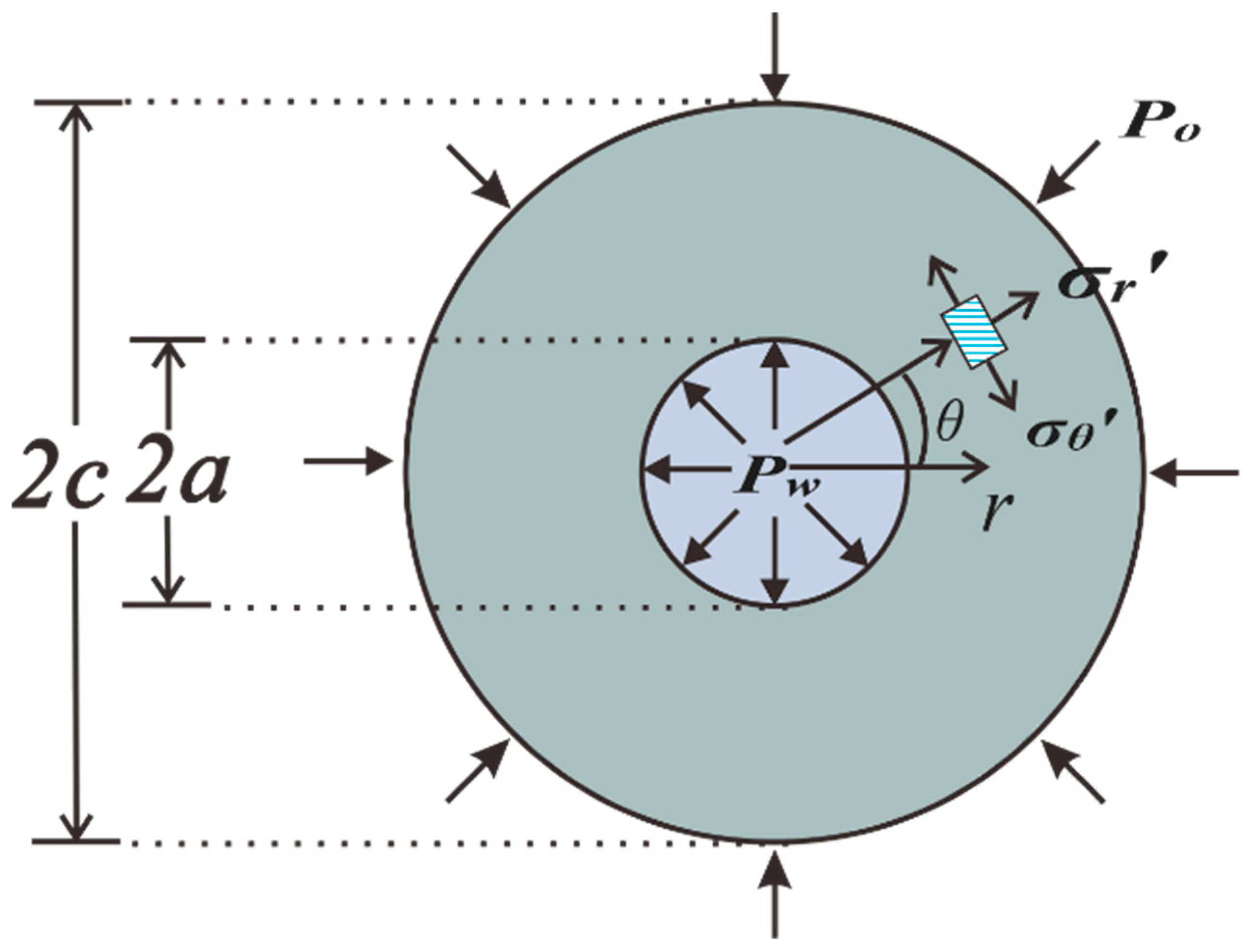
2.1. Fluid–Solid Coupling Model

To analyze the fluid–solid coupling effect around the open-hole wellbore under transient seepage conditions, this paper establishes a two-dimensional planar wellbore physical model. As shown in Figure 1, the wellbore has an inner radius of a and an outer radius of c, where r represents the distance from the wellbore axis, θ represents the angle, the water pressure at the inner boundary of the cylinder is P_w, and the initial pore pressure at the outer boundary is P_o. It is assumed that the rocks surrounding the open-hole wellbore are isotropic and homogeneous. Under the influence of the pressure difference between the inner and outer boundaries, fluid seeps radially from the wellbore into the pores of the reservoir rock. By establishing a polar coordinate system, this paper analyzes the effective radial stress σ’_r and ECS σ’_θ formed in the rock around the cylinder due to fluid action. (Note that in this paper, positive values are assigned to compressive stress, while negative values represent tensile stress).

For an open-hole wellbore, the stress equilibrium equation and stress boundary conditions satisfied by the surrounding rock when fluid seepage enters the rock pores are as follows [23]:

$$\begin{array}{ll}\frac{d{\sigma }_r^{\prime }}{dr}+\frac{{\sigma }_r^{\prime }-{\sigma }_{\theta }^{\prime }}{r}+\alpha \frac{dP}{dr}=0& \left(StressEquilibriumEquation\right)\\ \left\{\begin{array}{c}\begin{array}{cc}{\sigma }_r^{\prime }=P_w-\alpha P_w& r=a\end{array}\\ \begin{array}{cc}{\sigma }_r^{\prime }=P_o-\alpha P_o& r=c\end{array}\hfill \end{array}\right.& \left(StressBoundaryConditions\right)\end{array}$$

(1)

Here, α is the Biot effective stress coefficient and P represents the pore pressure. As shown in Equation (1), the effective stress field formed in the surrounding reservoir rock due to fluid action around the wellbore can be decomposed into the superposition of stress fields generated by both volume forces and surface forces, including: (1) internal and external boundary surface forces P_w − αP_w and P_o − αP_o; and (2) the seepage force term αdP/dr.

To establish a finite difference format, the first step is to create a stress function Φ to characterize the radial stress σ’_r and circumferential stress σ’_θ:

$$\left\{\begin{array}{c}{\sigma }_{\theta 2}^{\prime }=\frac{d\Phi }{dr}+r\alpha \frac{dP}{dr}\hfill \\ {\sigma }_{r2}^{\prime }=\frac{\Phi }{r}\hfill \end{array}\right.$$

(2)

Due to the axisymmetric nature of the stress field formed by fluid action around the wellbore, the geometric and physical equations satisfied by the rock surrounding the wellbore under fluid influence can be obtained using plane strain conditions:

$$\begin{array}{ll}\left\{\begin{array}{c}{\epsilon }_{\theta }=\frac{u_r}{r}\\ {\epsilon }_r=\frac{d{u}_r}{dr}\\ {\gamma }_{r\theta }=\frac{dr{\epsilon }_{\theta }}{dr}\end{array}\right.& \left(GeometricEquation\right)\\ \left\{\begin{array}{c}{\epsilon }_r=\frac{1}{E}\left[{\sigma }_r\left(1-{\nu }^2\right)-\nu \left(1+\nu \right){\sigma }_{\theta }\right]\\ {\epsilon }_{\theta }=\frac{1}{E}\left[{\sigma }_{\theta }\left(1-{\nu }^2\right)-\nu \left(1+\nu \right){\sigma }_r\right]\end{array}\right.& \left(PhysicalEquation\right)\end{array}$$

(3)

Combining Equation (2) with (3) and substituting them into Equation (1), we can derive the compatibility equation and boundary conditions satisfied by the stress function as follows:

$$\begin{array}{ll}{r}^2\frac{d^2\Phi }{d{r}^2}+r\frac{d\Phi }{dr}-\Phi +r^2\alpha \frac{\left(2+\nu -{\nu }^2\right)}{\left({\nu }^2-1\right)}\frac{\partial P}{\partial r}+r^3\alpha \frac{{\partial }^{2}P}{\partial r^2}=0& \left(CompatibilityEquation\right)\\ \left\{\begin{array}{l}\begin{array}{cc}\Phi =a\left(P_w-\alpha P_w\right)& r=a\end{array}\hfill \\ \begin{array}{cc}\Phi =c\left(P_o-\alpha P_o\right)& r=c\end{array}\hfill \end{array}\right.& \left(BoundaryConditions\right)\end{array}$$

(4)

To solve the compatibility equation, it is necessary to calculate the distribution of pore pressure around the wellbore under transient seepage conditions. In the Biot poroelastic consolidation theory [24,25], the governing equation for pore pressure propagation under the combined influence of solid deformation and fluid is as follows:

$$\left\{\begin{array}{c}\kappa {\nabla }^{2}P=\alpha \frac{\partial {\epsilon }_{kk}}{\partial t}+\frac{1}{Q}\frac{\partial P}{\partial t}\\ Q=\frac{2G\left({\nu }_u-\nu \right)}{{\alpha }^2\left(1-2\nu \right)\left(1-2{\nu }_u\right)}\end{array}\right.$$

(5)

In the equation, the parameters are defined as follows: Q is the Biot modulus, when α = 1 and only the seepage force is considered, Q = 1/ϕc_f, where ϕ is the porosity of the rock, and c_f is the fluid compressibility in Pa⁻¹. G is the shear modulus defined as G = E/2 (1 + ν), where E is the Young’s modulus in Pa and ν is the drained Poisson’s ratio. ν_u represents the undrained Poisson’s ratio. t is time measured in seconds. κ is the permeability coefficient defined as κ = k/μ, where k is the permeability in m² and μ is the fluid viscosity in Pa·s. ε_kk represents volumetric expansion.

To facilitate a convenient solution for the pore pressure propagation equation, Geertsma and Yew, among others [26,27], derived a conversion equation relating volumetric expansion (ɛ_kk) to pore pressure (P) based on the Biot consolidation theory:

$$\left\{\begin{array}{c}{\epsilon }_{kk}=c_{m}P\\ c_m=\frac{\alpha \left(1-2\nu \right)}{2G\left(1-\nu \right)}\end{array}\right.$$

(6)

By utilizing Equation (6) to process Equation (5), we can obtain the pore pressure propagation equation that takes into account the influence of solid deformation:

$${\nabla }^{2}P=\frac{1}{\kappa }\left(\alpha c_m+\frac{1}{Q}\right)\frac{\partial p}{\partial t}$$

(7)

The combination of the Compatibility Equation (4) and Pore Pressure Propagation Equation (7) forms the fundamental control equations for the transient fluid–solid coupling model around a bare wellbore under seepage conditions. By applying the finite difference method to discretize the above equations, we obtain:

$$\left\{\begin{array}{c}{r_i}^2\frac{{\Phi }_{i+1}+{\Phi }_{i-1}-2{\Phi }_i}{h^2}+r_i\frac{{\Phi }_{i+1}-{\Phi }_{i-1}}{2h}-{\Phi }_i-{r_i}^2\alpha \frac{\left(2+\nu -{\nu }^2\right)}{\left({\nu }^2-1\right)}\frac{P_{i+1}-P_{i-1}}{2h}+{r_i}^3\alpha \frac{P_{i+1}+P_{i-1}-2P_i}{h^2}=0\\ \begin{array}{c}\frac{P_{i+1}^{j+1}-2P_i^{j+1}+P_{i-1}^{j+1}}{h^2}+\frac{1}{r_i}\frac{P_{i+1}^{j+1}-P_{i-1}^{j+1}}{2h}=\beta \frac{P_i^{j+1}-P_i^j}{\Delta t}\\ \beta =\frac{1}{\kappa }\left(\alpha c_m+\frac{1}{Q}\right)\end{array}\\ r_i=h\cdot i+a i=0,1,2\dots n\\ t_j=\Delta t\cdot j j=0,1,2\dots m\end{array}\right.$$

(8)

where h is the iterative step size, h = c − a/n; Δt is the time step size; and (r_i, t_j) represents the grid nodes. The adopted time scheme is backward differencing. Since the solution area is two-dimensional and axially symmetric, there is no need to determine the unit type, just mesh the solution area. To solve Equation (8), we meshed the region within a certain radius around the open-hole wellbore, as illustrated in Figure 2.

Taking hydraulic fracturing as an example, according to the fracturing construction curve, the wellbore pressure can be considered to increase at a constant pressurization rate [28]. Meanwhile, at the far-field boundary, the pore pressure can be assumed to be the initial pore pressure. Therefore, the boundary conditions for the pore pressure propagation equation are as follows:

$$\left\{\begin{array}{cc}P\left(0,j\right)=C{t}_j+P_o\hfill & r=a\hfill \\ P\left(n,j\right)=P_o& r=c\hfill \end{array}\right.$$

(9)

where C represents the wellbore’s pressurization rate, MPa/s_o.

As indicated by the boundary conditions specified in Equation (9), the wellbore pressure is directly influenced by both the wellbore pressurization rate and time. Meanwhile, at the far-field outer boundary, the pore pressure remains constant and equal to the initial pore pressure.

According to the governing Equation (8) and boundary conditions 9, the tridiagonal matrix required to solve the stress function and pore pressure can be established. The tridiagonal matrix AX = B for pore pressure is:

$$\mathbf{A}=\left[\begin{array}{cccccc}\left(1+2A_1\right)& -\left(A_1+\frac{A_2}{r_1}\right)& 0& •& •& 0\\ \left(\frac{A_2}{r_2}-A_1\right)& \left(1+2A_1\right)& -\left(A_1+\frac{A_2}{r_2}\right)& •& •& 0\\ 0& •& •& •& •& •\\ •& •& •& •& •& •\\ •& •& •& \left(\frac{A_2}{r_{n-2}}-A_1\right)& \left(1+2A_1\right)& -\left(A_1+\frac{A_2}{r_{n-2}}\right)\\ 0& •& •& •& \left(\frac{A_2}{r_{n-1}}-A_1\right)& \left(1+2A_1\right)\end{array}\right]$$

(10)

where A₁ = Δt/(h²β); A₂ = Δt/(2hβ)

$$\mathbf{X}=\left[\begin{array}{c}{P}_1^{j+1}\\ P_2^{j+1}\\ •\\ •\\ •\\ P_{n-1}^{j+1}\end{array}\right]\mathbf{B}=\left[\begin{array}{c}{P}_1^j-\left(\frac{A_2}{r_1}-A_1\right)P_0^{j+1}\\ P_2^j\\ •\\ •\\ •\\ P_{n-1}^j+\left(A_1+\frac{A_2}{r_{n-1}}\right)P_n^{j+1}\end{array}\right]$$

(11)

The tridiagonal matrix that the stress function satisfies is CY = D:

$$\mathbf{C}=\left[\begin{array}{cccccc}\frac{-2{r_1}^2-h^2}{h^2}& \frac{2{r_1}^2+h{r}_1}{2h^2}& 0& •& •& 0\\ \frac{2{r_2}^2-h{r}_2}{2h^2}& \frac{-2{r_2}^2-h^2}{h^2}& \frac{2{r_2}^2+h{r}_2}{2h^2}& •& •& 0\\ 0& •& •& •& •& •\\ •& •& •& •& •& •\\ •& •& •& \frac{2{r_{n-2}}^2-h{r}_{n-2}}{2h^2}& \frac{-2{r_{n-2}}^2-h^2}{h^2}& \frac{2{r_{n-2}}^2+h{r}_{n-2}}{2h^2}\\ 0& •& •& •& \frac{2{r_{n-1}}^2-h{r}_{n-1}}{2h^2}& \frac{-2{r_{n-1}}^2-h^2}{h^2}\end{array}\right]$$

(12)

$$\mathbf{Y}=\left[\begin{array}{c}{\Phi }_1\\ {\Phi }_2\\ •\\ •\\ •\\ {\Phi }_{n-1}\end{array}\right]\mathbf{D}=\left[\begin{array}{c}\frac{{r_1}^3}{h^2}\alpha \left(P_2+P_0-2P_1\right)-\frac{{r_1}^2}{2h}\alpha \gamma \left(P_2-P_0\right)-\frac{2{r_1}^2+h{r}_1}{2h^2}\left(a{P}_o-a\alpha P_o\right)\\ \frac{{r_2}^3}{h^2}\alpha \left(P_3+P_1-2P_2\right)-\frac{{r_2}^2}{2h}\alpha \gamma \left(P_3-P_1\right)\\ •\\ •\\ •\\ \frac{{r_{n-1}}^3}{h^2}\alpha \left(P_n+P_{n-2}-2P_{n-1}\right)-\frac{{r_{n-1}}^2}{2h}\alpha \gamma \left(P_n-P_{n-2}\right)-\frac{2{r_{n-1}}^2+h{r}_2}{2h^2}\left(a{P}_n-a\alpha P_n\right)\end{array}\right]$$

(13)

Under the boundary conditions specified in Equation (9), we simultaneously solve the aforementioned matrices through programming to obtain the pore pressure field and stress function Subsequently, this stress function can be utilized to solve and acquire the stress field resulting from the fluid interactions around the wellbore under transient fluid–solid coupling conditions. During hydraulic fracturing, the effective circumferential stress directly affects the fracture initiation pressure [29], so subsequent chapters will only focus on the circumferential stress around the wellbore.

2.2. Model Validation

2.2.1. Pore Pressure Field Verification

When considering the absence of rock matrix particle compressibility (Biot coefficient α equals 1) and neglecting the influence of solid deformation on pore pressure, the pore bnpressure propagation Equation (7) can be simplified to:

$$\left\{\begin{array}{c}\frac{{\partial }^{2}P}{\partial r^2}+\frac{1}{r}\frac{\partial P}{\partial r}=\frac{1}{\chi }\frac{\partial P}{\partial t}\\ \chi =\frac{k}{\varphi \mu c_f}\end{array}\right.$$

(14)

where χ is the propagation coefficient, m²/s; this study assumes c_f = 4.5 × 10⁻¹⁰ Pa⁻¹.

Despite not accounting for the influence of solid deformation on pore pressure, Equation (14) remains a transient pore pressure propagation equation dependent on time. Based on Equation (14), Carslaw and Jaeger [30] derived an analytical solution for the radial distribution of pore pressure around a hollow cylindrical body under a constant pressurization rate:

$$P\left(r,t\right)=C{\displaystyle {\int }_o^{t}f\left(r,s\right)}ds$$

(15)

where:

$$f\left(r,t\right)=1+{\displaystyle {\int }_o^{\infty }\exp \left(-\chi u^{2}t\right)}\left[\frac{J_0\left(ur\right)Y_0\left(ua\right)-Y_0\left(ur\right)J_0\left(ua\right)}{J_0{\left(ua\right)}^2+Y_0{\left(ua\right)}^2}\right]\frac{du}{u}$$

(16)

J₀ and Y₀ are the first and second kinds of zero-order Bessel functions.

By adjusting the parameter β in the finite difference Equation (8) and comparing it with the analytical solution for the transient pore pressure distribution mentioned above, we can verify the accuracy of the difference format established in this work.

Figure 3 compares the analytical solution with the numerical solution of pore pressure distribution around the wellbore under a constant pressurization rate. It is evident from Figure 3 that, starting from the initial moment, the pore pressure distribution near the wellbore undergoes significant variations due to wellbore pressurization. As one moves away from the wellbore, the distribution gradually approaches the initial pore pressure before pressurization.

At different time instances, the analytical solution for transient pore pressure and the numerical solution presented in this study demonstrate a close agreement, with the relative error limited to less than 0.1%. This validation confirms the accuracy of the transient fluid–solid coupling model established in this paper.

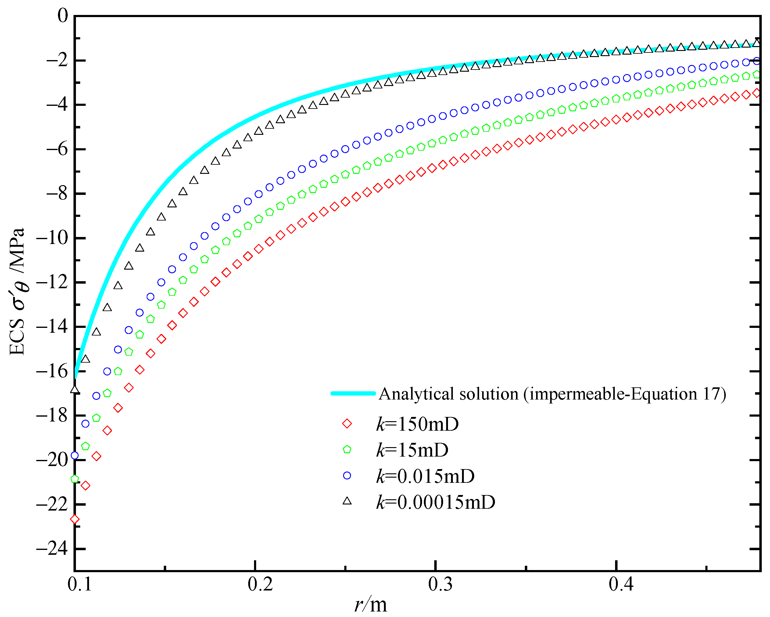
2.2.2. Effective Stress Field Verification

There is no analytical solution available for the stress field around the wellbore under transient seepage conditions. However, an analytical solution does exist for the stress field around the wellbore in the case of impermeable reservoirs. When the rock is impermeable, the ECS σ’_θ induced by the fluid pressures (P_w and P_o) at the inner and outer boundaries of the wellbore can be calculated using the Lame formula and Terzaghi’s principle of effective stress [31,32,33].

$${\sigma }_{\theta }^{\prime }=\left[\frac{a^2{c}^2\left(P_o-P_w\right)}{c^2-a^2}\frac{1}{r^2}-\frac{a^2{P}_w-c^2{P}_o}{c^2-a^2}\right]-P_o$$

(17)

When c >> a, Equation (17) can be simplified to $\frac{a^2}{r^2}\left(P_o-P_w\right)$.

By varying the reservoir’s permeability, we employed the finite difference scheme detailed in Section 2.1 to compute the effective circumferential stress resulting from the fluid flow around the wellbore during transient seepage. We investigated the variations in the transient stress field surrounding the wellbore as the reservoir’s permeability gradually decreased, eventually reaching impermeability. As depicted in Figure 4, the results obtained from the numerical solution are compared with those derived from the analytical solution provided by Equation (17).

In the case of an impermeable reservoir, the seepage force term in Equation (1) is negligible, and the fluid primarily exerts a surface force on the rocks surrounding the wellbore. As depicted in Figure 4, for impermeable reservoirs, the effective circumferential stress resulting from fluid interaction around the wellbore is tensile stress. However, when fluid seepage enters the reservoir, the effective circumferential tensile stress induced by the fluid around the wellbore, due to the seepage force, increases significantly. A greater effective circumferential tensile stress increases the susceptibility of the well wall to tensile failure. This demonstrates that the seepage force significantly increases the possibility of tensile failure of the wellbore wall. Under identical injection conditions, an increasing reservoir fluid permeability amplifies the seepage effect, leading to a higher effective circumferential tensile stress around the wellbore.

As the reservoir’s permeability gradually diminishes, the numerical solution begins to converge toward the analytical solution. When the reservoir’s permeability approaches an impermeable state, the analytical and numerical solution curves essentially overlap. This confirms the stability and accuracy of the finite difference scheme presented in this article for computing the effective circumferential stress field.

3. Numerical Results

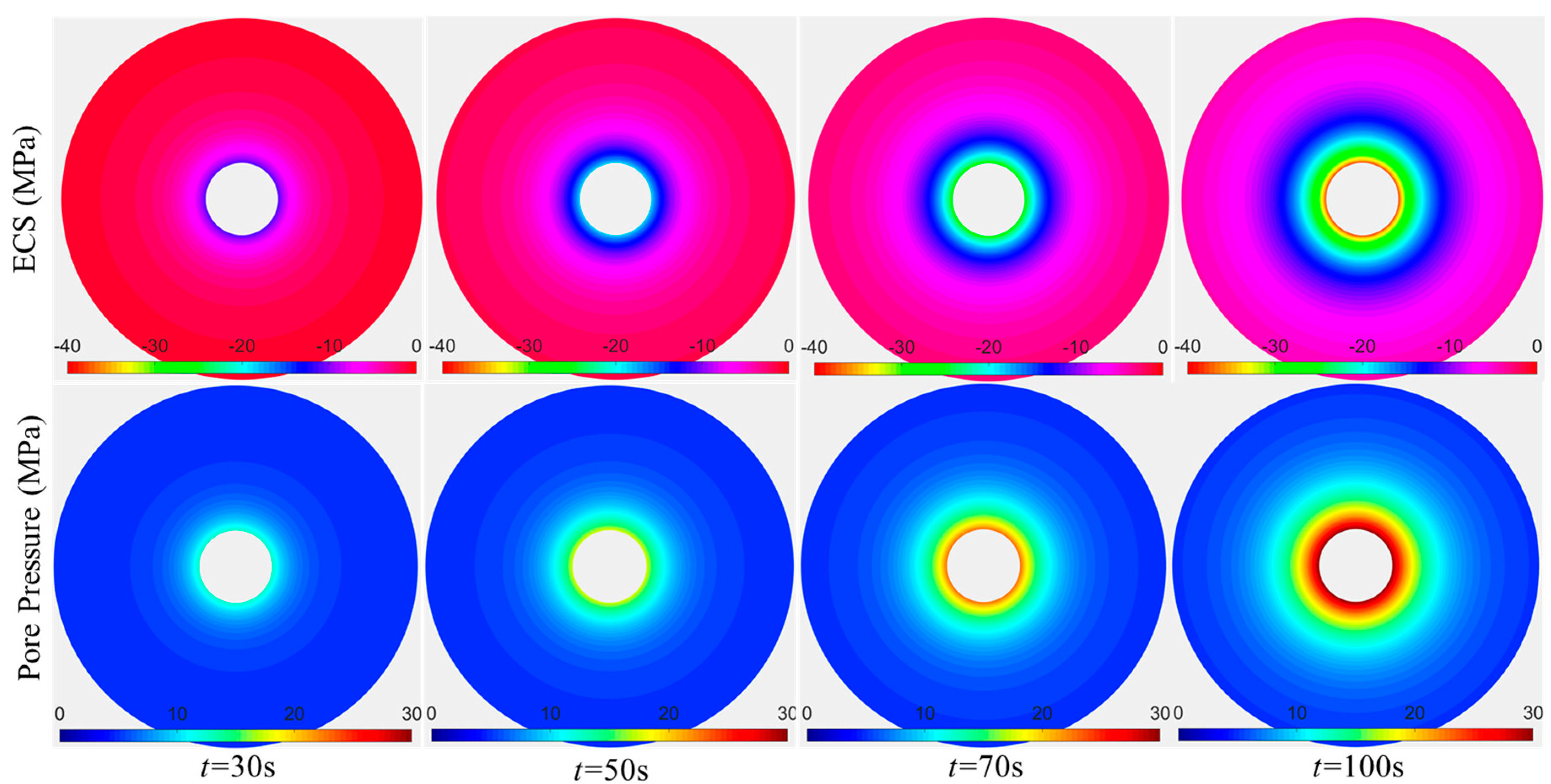
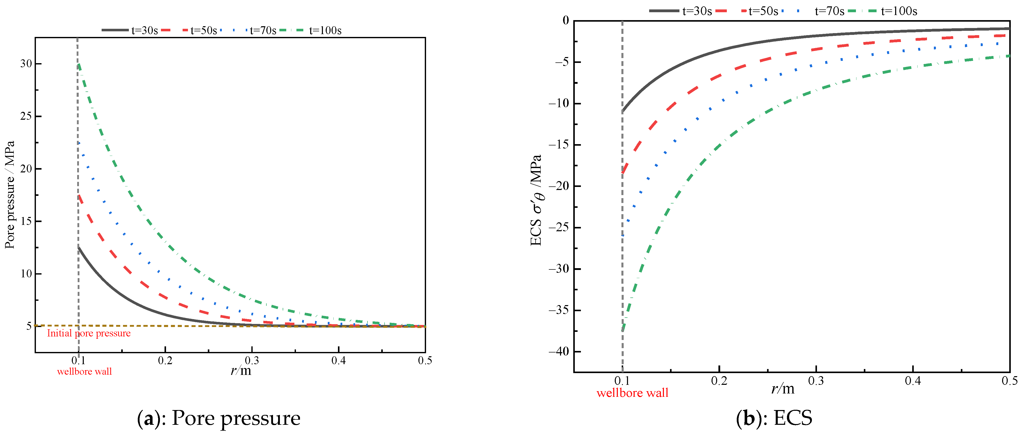
3.1. Evolution Characteristics of Pore Pressure Field and Effective Stress Field

In this section, α is set to 1, resulting in the disappearance of the surface force term in Equation (1), with fluid exerting only seepage force on the rock framework. Figure 5 illustrates pseudo-color plots of the pore pressure field and the corresponding ECS field around the wellbore at different time steps during the stable pressurization process of hydraulic fracturing. It shows the variations in pore pressure and ECS along the radial direction (C = 0.25 MPa/s, μ = 10 mPa·s, K = 0.1 mD, ϕ = 0.1, P₀ = 5 MPa, a = 0.1 m, C = 0.5 m, ν = 0.25, and E = 5.0 × 10⁴ MPa).

By combining the observations from Figure 5 and Figure 6, it becomes evident that significant changes occur in the pore pressure field around the wellbore and the Effective Circumferential Stress (ECS) field formed by the action of seepage forces during the stable pressurization process of the wellbore. The pore pressure and ECS near the wellbore exhibit larger variations over time, while moving away from the wellbore results in a rapid decrease in pore pressure towards the initial pore pressure state. Under transient fluid–solid coupling conditions, the ECS formed by the action of seepage forces is maximized near the wellbore and gradually diminishes towards zero with an increasing distance from the wellbore. The magnitude of changes in the ECS due to seepage forces is more pronounced in the vicinity of the wellbore.

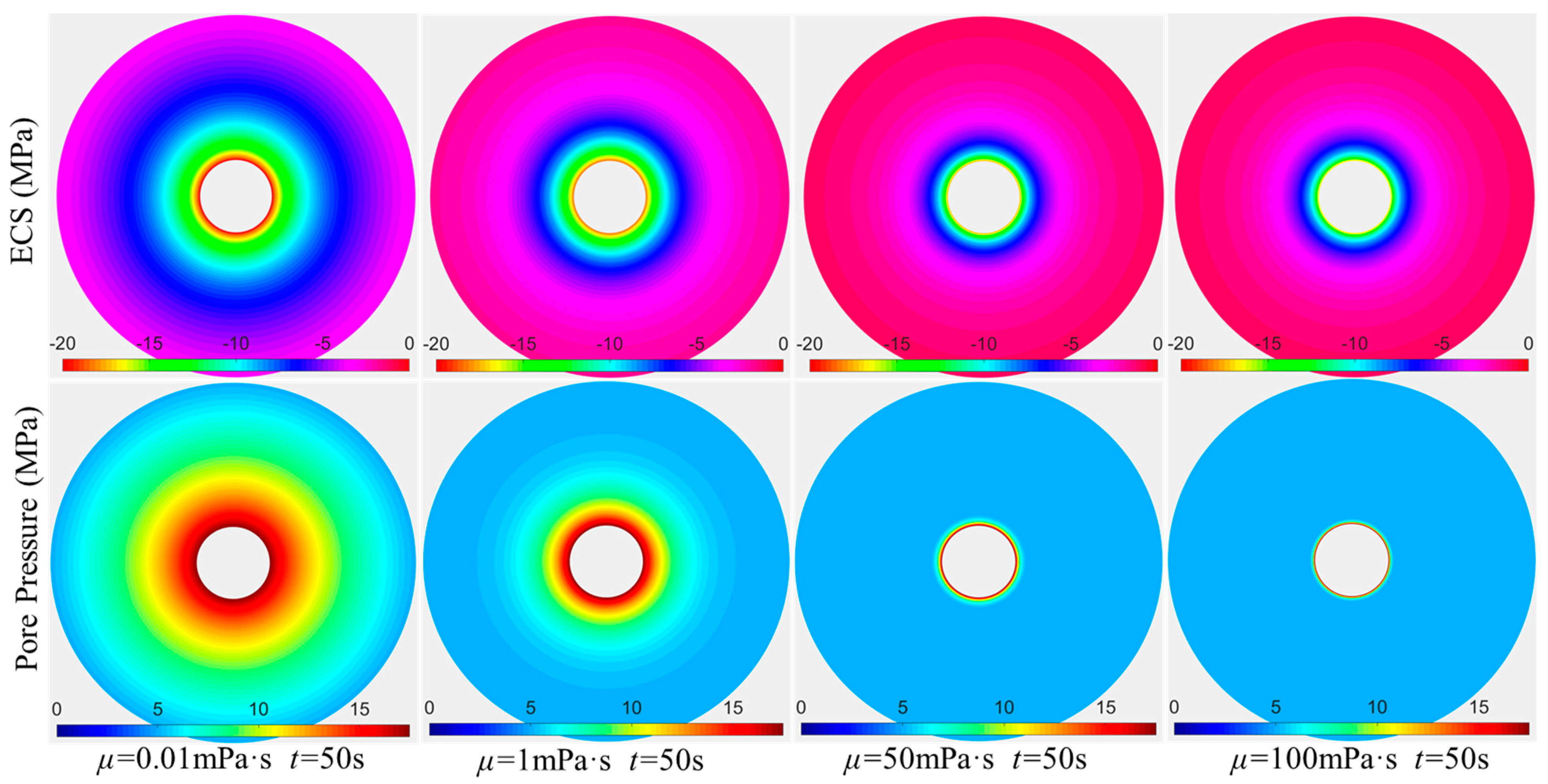
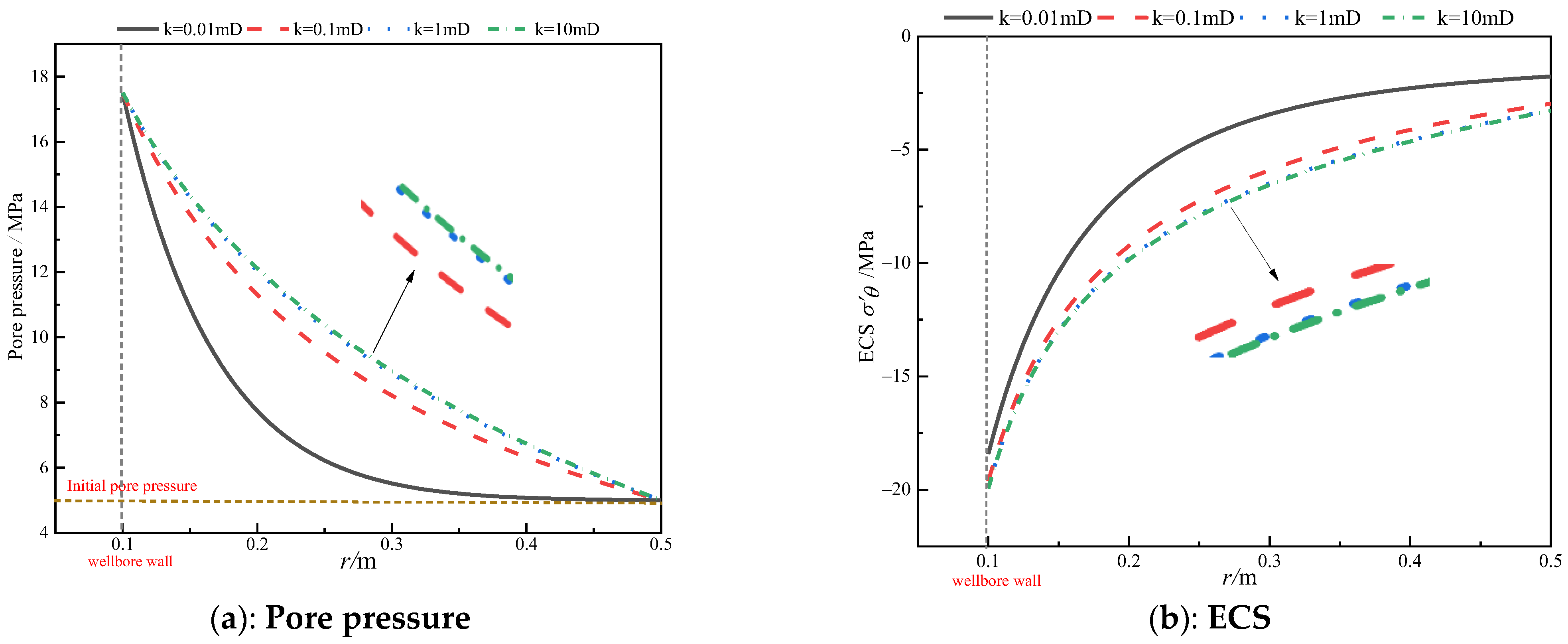
3.2. Influence of Seepage Parameters

Using the established transient fluid–solid coupling model, an analysis of two key parameters, fluid viscosity and wellbore pressurization rate, was conducted. Figure 7 presents pseudo-color plots of the pore pressure field around the wellbore and the corresponding ECS field formed by fluid action at the same time step but with varying fluid viscosities. Figure 8 displays pseudo-color plots of the pore pressure field and ECS field when the wellbore pressure is pressurized to the same level using different pressurization rates (α = 1; ν = 0.25, E = 5.0 × 10⁴ MPa, K = 0.1 mD, ϕ = 0.1, and P₀ = 5 MPa).

In Figure 7, it is evident that the fluid viscosity has a significant impact on the pore pressure field around the wellbore and the ECS field formed by seepage forces under transient conditions. At the same time step, when the fluid viscosity is high, the pore pressure rapidly decreases to the initial pore pressure state around the wellbore as fluid seeps into the reservoir. Conversely, as the fluid viscosity decreases, the pore pressure distribution around the wellbore gradually becomes smoother. Additionally, with a decreasing fluid viscosity, the ECS field formed by seepage forces around the wellbore significantly strengthens, resulting in a notable increase in effective circumferential tensile stress values. Therefore, for low-permeability reservoirs, reducing fluid viscosity can significantly enhance the action of seepage forces around the wellbore.

Figure 8 demonstrates that, when pressurized to the same pressure level, the pressurization rate significantly affects the pore pressure field and ECS field. A smaller wellbore pressurization rate results in a longer time required to reach the same pressure level, but leads to higher pore pressure values around the wellbore. Conversely, a higher pressurization rate leads to a faster decline in the pore pressure around the wellbore. Additionally, as the pressurization rate decreases, the ECS values formed by seepage forces around the wellbore gradually increase. Therefore, a lower pressurization rate results in higher ECS values formed by seepage forces around the wellbore when pressurized to the same pressure level. Consequently, for reservoirs with a lower permeability, it may be advisable to consider lower fluid injection rates to enhance the action of seepage forces.

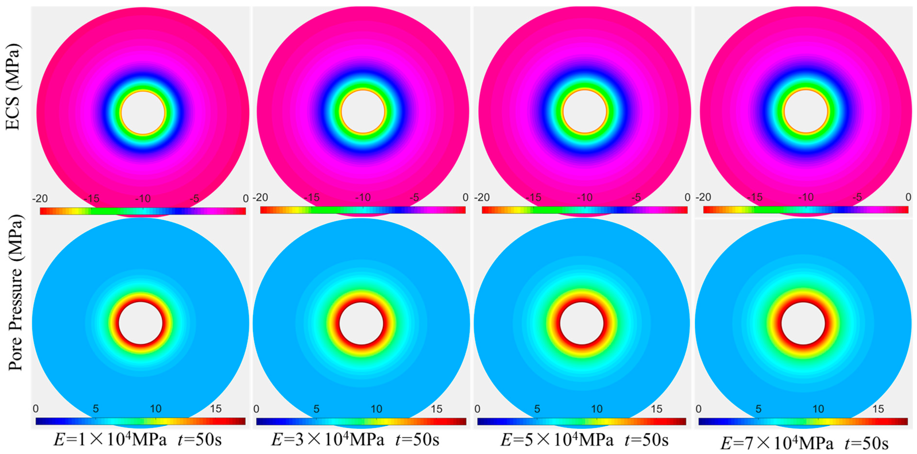
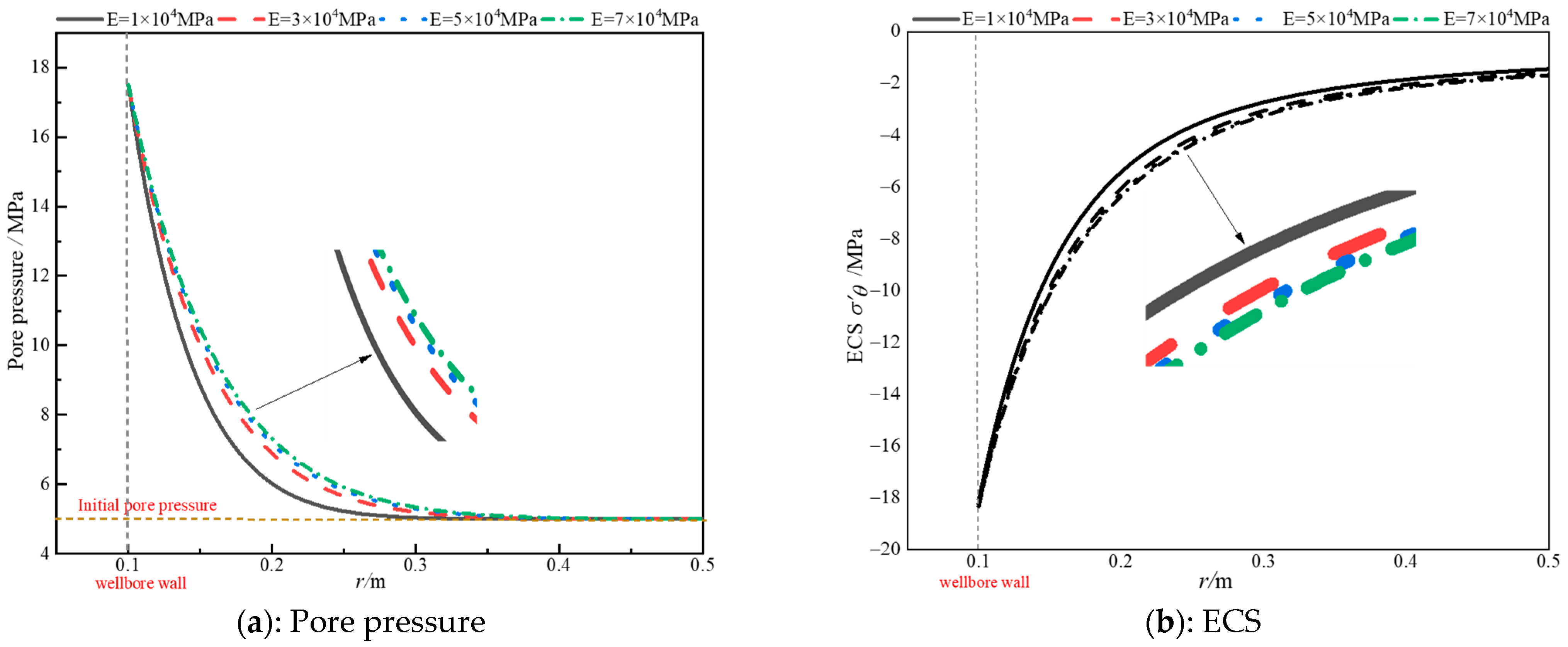
3.3. Influence of Reservoir Parameters

Using the transient fluid–solid coupling model established in this study, we can analyze the effects of key reservoir parameters, such as reservoir permeability and rock mechanics, on the pore pressure field around the wellbore and the ECS field formed by seepage forces (α = 1, μ = 1 mPa·s, ϕ = 0.1, P₀ = 5 MPa, and C = 0.25 MPa/s).

Figure 9 illustrates pseudo-color plots of the pore pressure field and ECS field under different reservoir permeability conditions, while Figure 10 shows the corresponding variations in the pore pressure and ECS along the radial direction. Combining the observations from Figure 8 and Figure 9, it becomes apparent that, under low-viscosity fluid conditions, decreasing the reservoir permeability amplifies the magnitude of pore pressure variations. Near the wellbore, a lower reservoir permeability leads to a faster decay in pore pressure. In the simulation case depicted in Figure 10, with low-viscosity fluid, once the reservoir permeability exceeds 1 mD, the pore pressure distribution tends toward a steady-state linear Darcy seepage distribution, and the influence of permeability on the pore pressure field and ECS field gradually diminishes. Consequently, under low-viscosity fluid conditions, a higher reservoir permeability results in elevated pore pressure values around the wellbore and increased ECS values formed by seepage forces.

Figure 11 and Figure 12 present pseudo-color plots illustrating the pore pressure field around the wellbore and the ECS field formed by seepage forces under varying conditions of Young’s modulus and Poisson’s ratio. Correspondingly, Figure 13 and Figure 14 provide radial profiles of the pore pressure and ECS along the radius.

Combining the observations from Figure 11, Figure 12, Figure 13 and Figure 14 reveals that, under fluid–solid coupling conditions, the elastic deformation of rock elements significantly affects the pore pressure field around the wellbore and the ECS field formed by seepage forces. Higher values of Young’s modulus and Poisson’s ratio result in elevated pore pressure values around the wellbore, corresponding to higher ECS values formed by seepage forces. Overall, Young’s modulus (E) has a slightly greater influence on the pore pressure field and the stress field formed by seepage forces than Poisson’s ratio (ν). However, compared to seepage parameters, rock mechanics parameters have a much weaker impact on the pore pressure field and the ECS field formed by seepage forces around the wellbore. In this paper, there is still room for improvement. Future research will delve into the analysis of well wall behavior, specifically in terms of tensile or shear failure, induced by fluid injection. This analysis will be based on the fluid–solid coupling model presented here, combined with rock failure criteria.

4. Conclusions

Based on the Biot consolidation theory and finite difference method, this paper established a transient fluid–solid coupling model that can analyze the stress field and pore pressure field around an open-hole wellbore during the initiation of hydraulic fractures. The transient analytical solution of the pore pressure field was used to verify the accuracy of the model and the stability of the calculation method. Using this model, this paper analyzed the effects of reservoir parameters and seepage parameters on open-hole wellbore fluid–solid coupling under different injection conditions. The simulation results show that:

(1) During the stable pressurization of the wellbore, significant changes were observed in the pore pressure field and effective stress field near the wellbore. As the distance from the wellbore increased to more than four times the radius, the fluid–solid coupling effect around the wellbore substantially diminished, returning to its initial state.

(2) With a decrease in fluid viscosity and wellbore pressurization rate, the pore pressure and ECS around the wellbore increased. Adjusting the fluid viscosity and wellbore pressurization rate allowed control over the action of seepage forces during wellbore fluid injection.

(3) Under conditions of low-viscosity fluid injection, a higher reservoir permeability yielded larger pore pressure values around the wellbore, accompanied by increased ECS values generated by seepage forces.

(4) When the Young’s modulus and Poisson’s ratio of the rock surrounding the wellbore were large, the pore pressure field and ECS were stronger. Notably, the Young’s modulus exhibited a more pronounced impact on the fluid–solid coupling effect around the wellbore compared to Poisson’s ratio.

References

1. Hasan, M.M.F.; First, E.L.; Boukouvala, F.; Floudas, C.A. A multi-scale framework for CO2 capture, utilization, and sequestration: CCUS and CCU. Comput. Chem. Eng. 2015, 81, 2–21. [Google Scholar] [CrossRef]
2. Jiang, K.; Ashworth, P.; Zhang, S.; Liang, X.; Sun, Y.; Angus, D. China’s carbon capture, utilization and storage (CCUS) policy: A critical review. Renew. Sustain. Energy Rev. 2020, 119, 109601. [Google Scholar] [CrossRef]
3. Pan, L.; Oldenburg, C.; Pruess, K.; Wu, Y.-S. Transient CO2 leakage and injection in wellbore-reservoir systems for geologic carbon sequestration. Greenh. Gases Sci. Technol. 2011, 1, 335–350. [Google Scholar] [CrossRef]
4. Zhu, H.; Deng, J.; Jin, X.; Hu, L.; Luo, B. Hydraulic Fracture Initiation and Propagation from Wellbore with Oriented Perforation. Rock Mech. Rock Eng. 2015, 48, 585–601. [Google Scholar] [CrossRef]
5. Zhou, D.; Wang, H.; He, Z.; Liu, Y.; Liu, S.; Ma, X.; Cai, W.; Bao, J. Numerical study of the influence of seepage force on the stress field around a vertical wellbore. Eng. Appl. Comput. Fluid Mech. 2020, 14, 1489–1500. [Google Scholar] [CrossRef]
6. Wang, H.; Zhou, D.; Liu, S.; Wang, X.; Ma, X.; Yao, T. Hydraulic fracture initiation for perforated wellbore coupled with the effect of fluid seepage. Energy Rep. 2022, 8, 10290–10298. [Google Scholar] [CrossRef]
7. Roy, P.; Morris, J.P.; Walsh, S.D.C.; Iyer, J.; Carroll, S. Effect of thermal stress on wellbore integrity during CO2 injection. Int. J. Greenh. Gas Control 2018, 77, 14–26. [Google Scholar] [CrossRef]
8. Haimson, B.; Fairhurst, C. Initiation and Extension of Hydraulic Fractures in Rocks. Soc. Pet. Eng. J. 1967, 7, 310–318. [Google Scholar] [CrossRef]
9. Haimson, B.C. Hydraulic Fracturing in Porus and Nonporus Rock and Its Potential for Determining In-Situ Stresses at Great Depth; University of Minnesota: Minneapolis, MN, USA, 1968. [Google Scholar]
10. Haimson, B.; Fairhurst, C. Hydraulic Fracturing in Porous-Permeable Materials. J. Pet. Technol. 1969, 21, 811–817. [Google Scholar] [CrossRef]
11. Hubbert, M.K.; Willis, D.G. Mechanics of Hydraulic Fracturing. Trans. AIME 1957, 210, 153–168. [Google Scholar] [CrossRef]
12. Reisabadi, M.Z.; Haghighi, M.; Sayyafzadeh, M.; Khaksar, A. Effect of matrix shrinkage on wellbore stresses in coal seam gas: An example from Bowen Basin, east Australia. J. Nat. Gas Sci. Eng. 2020, 77, 103280. [Google Scholar] [CrossRef]
13. Li, Y.; Cheng, Y.; Yan, C.; Song, L.; Liu, H.; Tian, W.; Ren, X. Mechanical study on the wellbore stability of horizontal wells in natural gas hydrate reservoirs. J. Nat. Gas Sci. Eng. 2020, 79, 103359. [Google Scholar] [CrossRef]
14. Ren, K.; Cai, C. Numerical Investigation into the Distributions of Temperature and Stress around Wellbore during the Injection of Cryogenic Liquid Nitrogen into Hot Dry Rock Reservoir. Math. Probl. Eng. 2021, 2021, 9913321. [Google Scholar] [CrossRef]
15. Jafari Raad, S.M.; Lawton, D.; Maidment, G.; Hassanzadeh, H. Transient non-isothermal coupled wellbore-reservoir modeling of CO2 injection—Application to CO2 injection tests at the CaMI FRS site, Alberta, Canada. Int. J. Greenh. Gas Control 2021, 111, 103462. [Google Scholar] [CrossRef]
16. Qiu, Y.; Ma, T.; Liu, J.; Peng, N.; Ranjith, P.G. Poroelastic response of inclined wellbore geometry in anisotropic dual-medium/media. Int. J. Rock Mech. Min. Sci. 2023, 170, 105560. [Google Scholar] [CrossRef]
17. Xiao, H.; Li, W.; Wang, Z.; Yang, S.; Tan, P. Critical Conditions for Wellbore Failure during CO2-ECBM Considering Sorption Stress. Sustainability 2023, 15, 3696. [Google Scholar] [CrossRef]
18. Rim, H.; Chen, Y.; Tokgo, J.; Du, X.; Li, Y.; Wang, S. Time-Dependent Effect of Seepage Force on Initiation of Hydraulic Fracture around a Vertical Wellbore. Materials 2023, 16, 2012. [Google Scholar] [CrossRef]
19. Hou, L.; Zhou, L.; Elsworth, D.; Wang, S.; Wang, W. Prediction of Fracturing Pressure and Parameter Evaluations at Field Practical Scales. Rock Mech. Rock Eng. 2024, 1–14. [Google Scholar] [CrossRef]
20. Hossain, M.M.; Rahman, M.K.; Rahman, S.S. Hydraulic fracture initiation and propagation: Roles of wellbore trajectory, perforation and stress regimes. J. Pet. Sci. Eng. 2000, 27, 129–149. [Google Scholar] [CrossRef]
21. Fallahzadeh, S.H.; Shadizadeh, S.R.; Pourafshary, P. Dealing with the Challenges of Hydraulic Fracture Initiation in Deviated-Cased Perforated Boreholes. In Proceedings of the Trinidad and Tobago Energy Resources Conference, Port of Spain, Trinidad and Tobago, 27–30 June 2010. [Google Scholar]
22. Ding, Y.; Liu, X.; Luo, P. The analytical model of hydraulic fracture initiation for perforated borehole in fractured formation. J. Pet. Sci. Eng. 2018, 162, 502–512. [Google Scholar] [CrossRef]
23. Wang, H.Y.; Zhou, D.S.; Gao, Q.; Fan, X.; Xu, J.Z.; Liu, S. Study on the Seepage Force-Induced Stress and Poroelastic Stress by Flow Through Porous Media Around a Vertical Wellbore. Int. J. Appl. Mech. 2021, 13, 2150065. [Google Scholar] [CrossRef]
24. Biot, M.A. General theory of three-dimensional consolidation. J. Appl. Phys. 1941, 12, 155–164. [Google Scholar] [CrossRef]
25. Rice, J.R.; Cleary, M.P. Some basic stress diffusion solutions for fluid-saturated elastic porous media with compressible constituents. Rev. Geophys. 1976, 14, 227–241. [Google Scholar] [CrossRef]
26. Geertsma, J. Problems of Rock Mechanics in Petroleum Production Engineering. In Proceedings of the 1st ISRM Congress, Lisbon, Portugal, 25 September–1 October 1966. [Google Scholar]
27. Yew, C.H.; Liu, G. Pore Fluid and Wellbore Stabilities. In Proceedings of the International Meeting on Petroleum Engineering, Beijing, China, 24–27 March 1992. [Google Scholar]
28. Ito, T. Effect of pore pressure gradient on fracture initiation in fluid saturated porous media: Rock. Eng. Fract. Mech. Eng. Fract. Mech. 2008, 75, 1753–1762. [Google Scholar] [CrossRef]
29. Wang, H.; Zhou, D. Mechanistic study on the effect of seepage force on hydraulic fracture initiation. Fatigue Fract. Eng. Mater. Struct. 2024. [Google Scholar] [CrossRef]
30. Carslaw, H.S.; Jaeger, J.C. Conduction of Heat in Solids; Clarendon Press: Oxford, UK, 1959; pp. 314–332. [Google Scholar]
31. Terzaghi, K.; Peck, R.B.; Mesri, G. Soil Mechanics in Engineering Practice, 3rd ed.; John Wiley: New York, NY, USA, 1995; 750p. [Google Scholar]
32. Chen, X.; Li, Y.; Liu, Z.; Tang, Y.; Sui, M. Visualized investigation of the immiscible displacement: Influencing factors, improved method, and EOR effect. Fuel 2023, 331, 125841. [Google Scholar] [CrossRef]
33. Hou, L.; Ren, J.; Fang, Y.; Cheng, Y. Data-driven optimization of brittleness index for hydraulic fracturing. Int. J. Rock Mech. Min. Sci. 2022, 159, 105207. [Google Scholar] [CrossRef]
Figure 1. Two-dimensional planar wellbore physical model.
Processes 12 00412 g001
Figure 2. Schematic diagram of grid nodes.
Processes 12 00412 g002
Figure 3. Comparison of radial distribution of pore pressure between analytical solution and numerical solution (χ = 2.2 × 10⁻⁴ m2/s, C = 0.5 MPa/s, P0 = 2.5 MPa).
Processes 12 00412 g003
Figure 4. Change in ECS σ’θ along the radial direction for different permeability (numerical and analytical solutions). C = 0.15 MPa/s; μ = 100 mPa·s; α = 1; t = 100 s; P0 = 5.0 MPa; ν = 0.25; and E = 5.0 × 10⁴ MPa.
Processes 12 00412 g004
Figure 5. Pseudo-color maps of pore pressure field and ECS field at different time steps.
Processes 12 00412 g005
Figure 6. Variation in radial pore pressure and ECS with radius at different time steps.
Processes 12 00412 g006
Figure 7. Pseudo-color maps of pore pressure field and stress field under different fluid viscosities (C = 0.25 MPa/s).
Processes 12 00412 g007
Figure 8. Pseudo-color maps of pore pressure field and ECS field under different pressurization rates (μ = 10 mPa·s).
Processes 12 00412 g008
Figure 9. Pseudo-color maps of pore pressure field and stress field under different reservoir permeability (E = 5.0 × 10⁴ MPa; ν = 0.25).
Processes 12 00412 g009
Figure 10. Radial pore pressure and ECS change with radius under different reservoir permeability conditions.
Processes 12 00412 g010
Figure 11. Pseudo-color maps of pore pressure field and stress field under different Young’s moduli (K = 0.1 mD; ν = 0.25).
Processes 12 00412 g011
Figure 12. Variation in pore pressure and ECS in the radial direction with radius under different Young’s modulus conditions.
Processes 12 00412 g012
Figure 13. Pseudo-color maps of pore pressure field and ECS field under different Poisson’s ratio conditions (K = 0.1 mD; E = 5.0 × 10⁴ MPa).
Processes 12 00412 g013
Figure 14. Variation in pore pressure and ECS in the radial direction with radius at different Poisson’s ratios.
Processes 12 00412 g014
Disclaimer/Publisher’s Note: The statements, opinions and data contained in all publications are solely those of the individual author(s) and contributor(s) and not of MDPI and/or the editor(s). MDPI and/or the editor(s) disclaim responsibility for any injury to people or property resulting from any ideas, methods, instructions or products referred to in the content.