


A Comparative Study of Oil–Water Two-Phase Flow Pattern Prediction Based on the GA-BP Neural Network and Random Forest Algorithm

Abstract
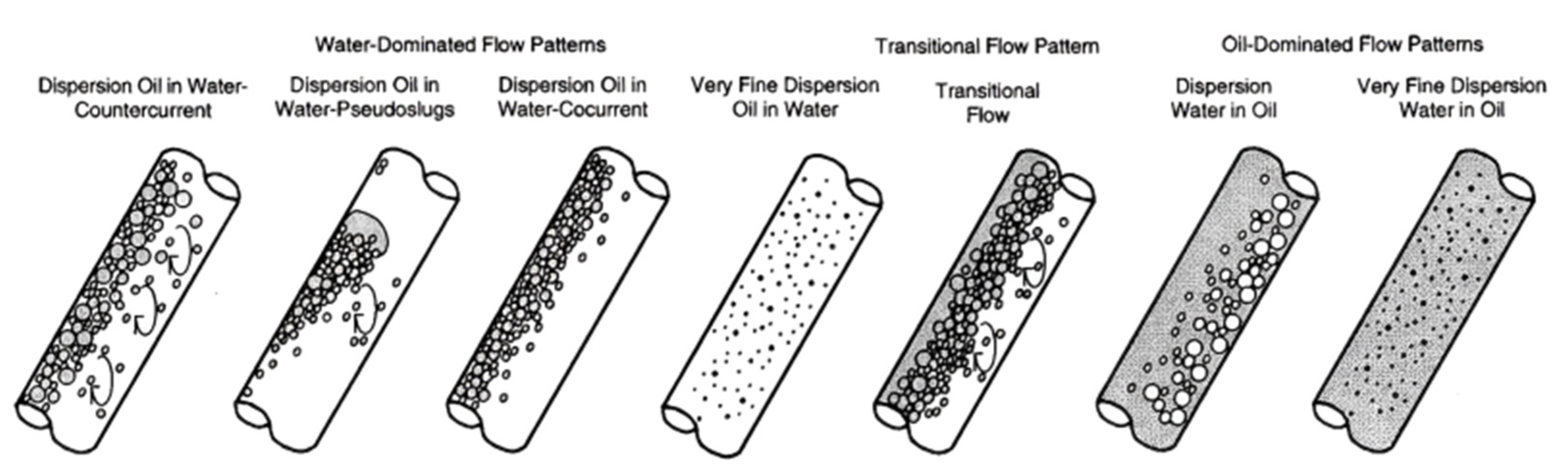
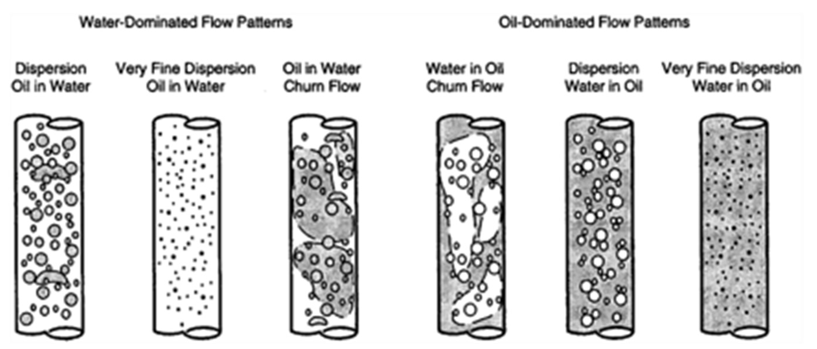
:1. Introduction
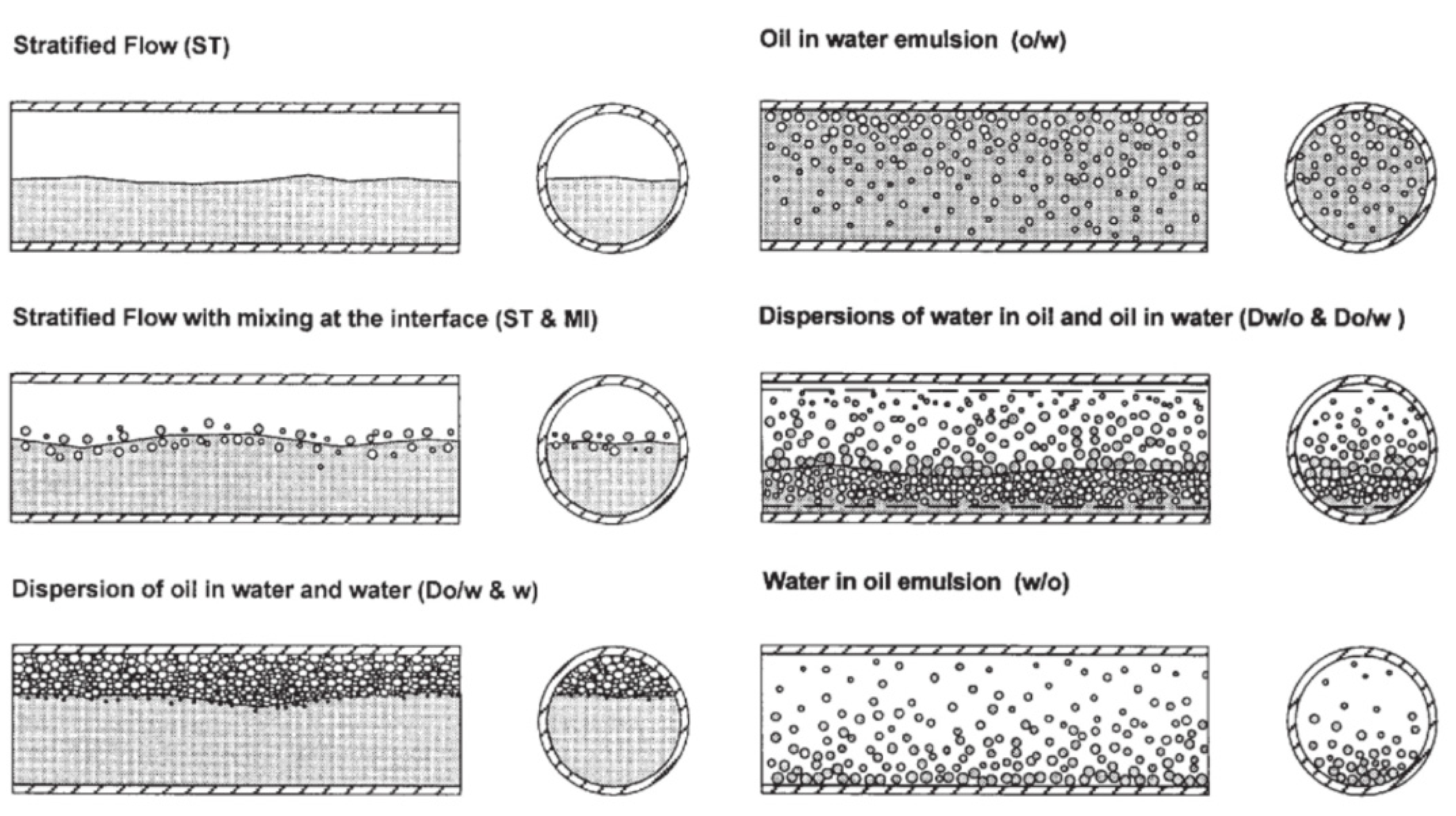
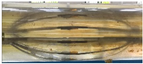
- bubble flow (water is a continuous phase).
- slug flow (water is a continuous phase).
- froth flow (no fixed continuous phase).
- mist flow (oil is a continuous phase).
2. Algorithmic Principle
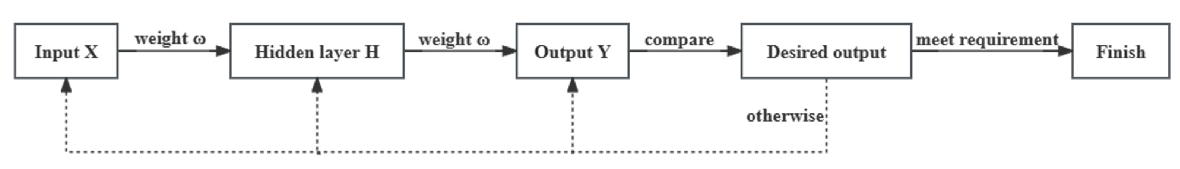
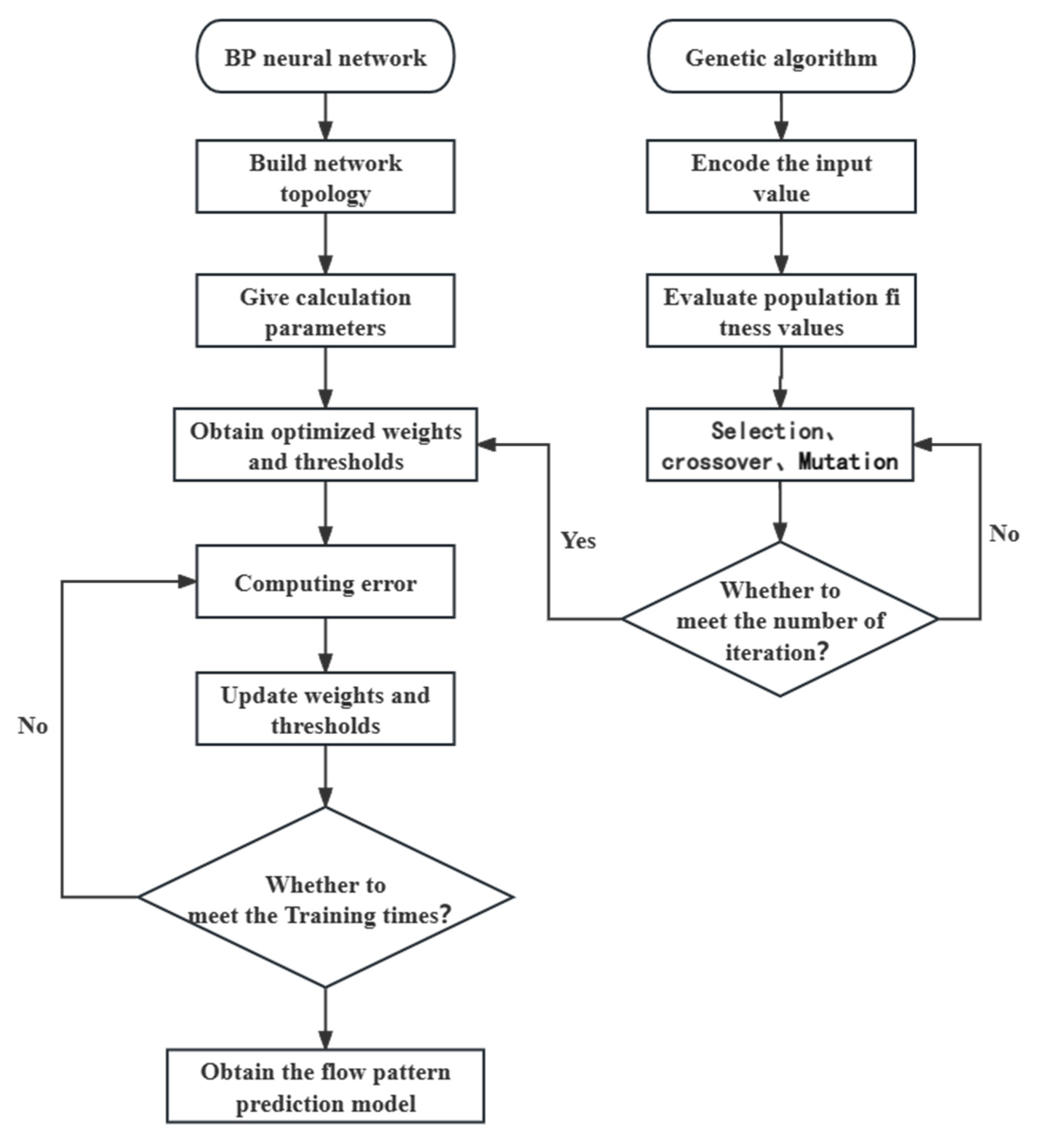
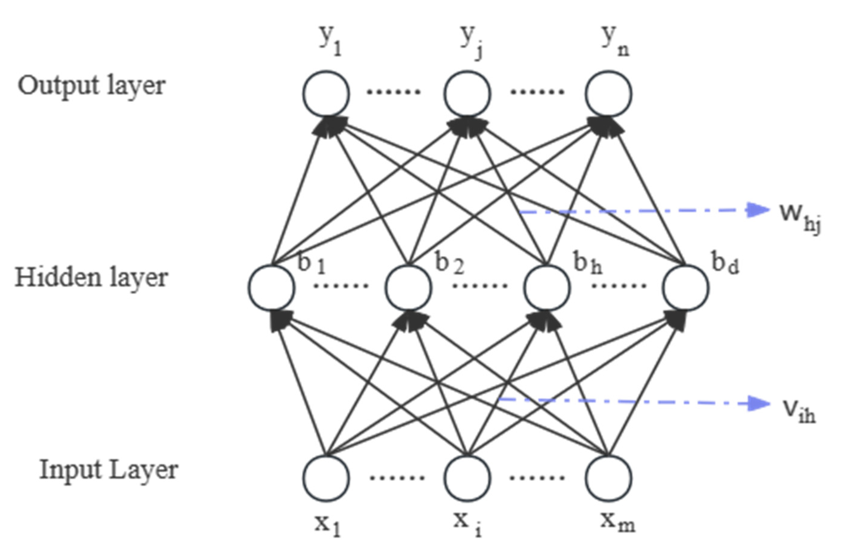
2.1. GA-BP Neural Networks
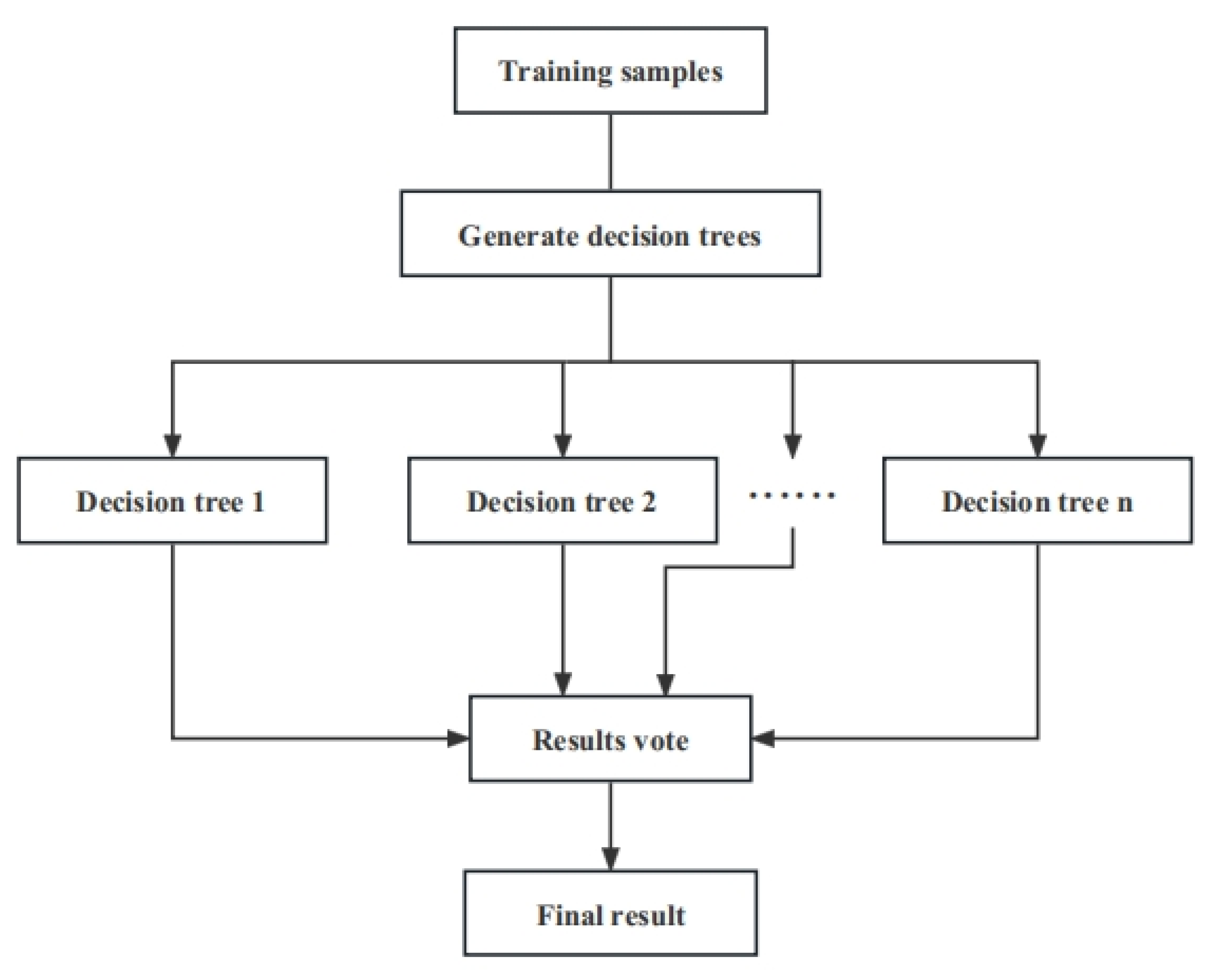
2.2. Random Forest Algorithm
3. Method Applications
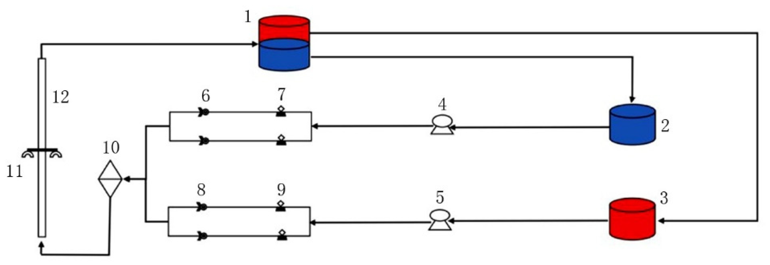
4. Experiment Overview
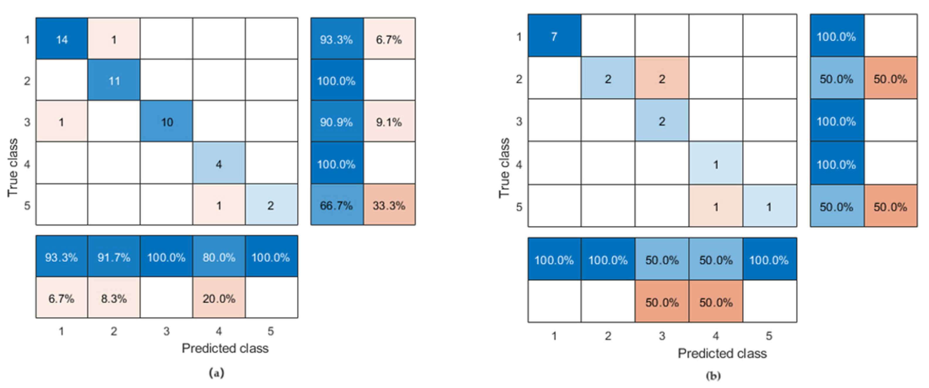
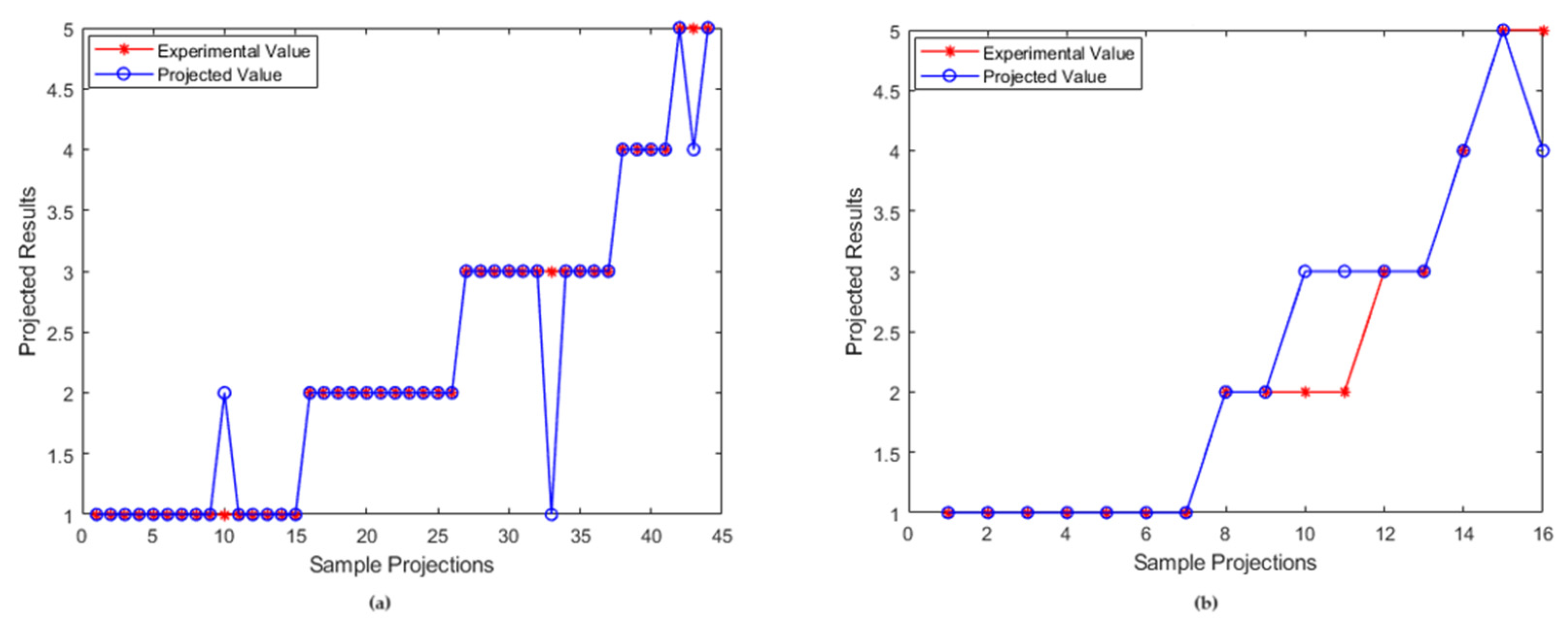
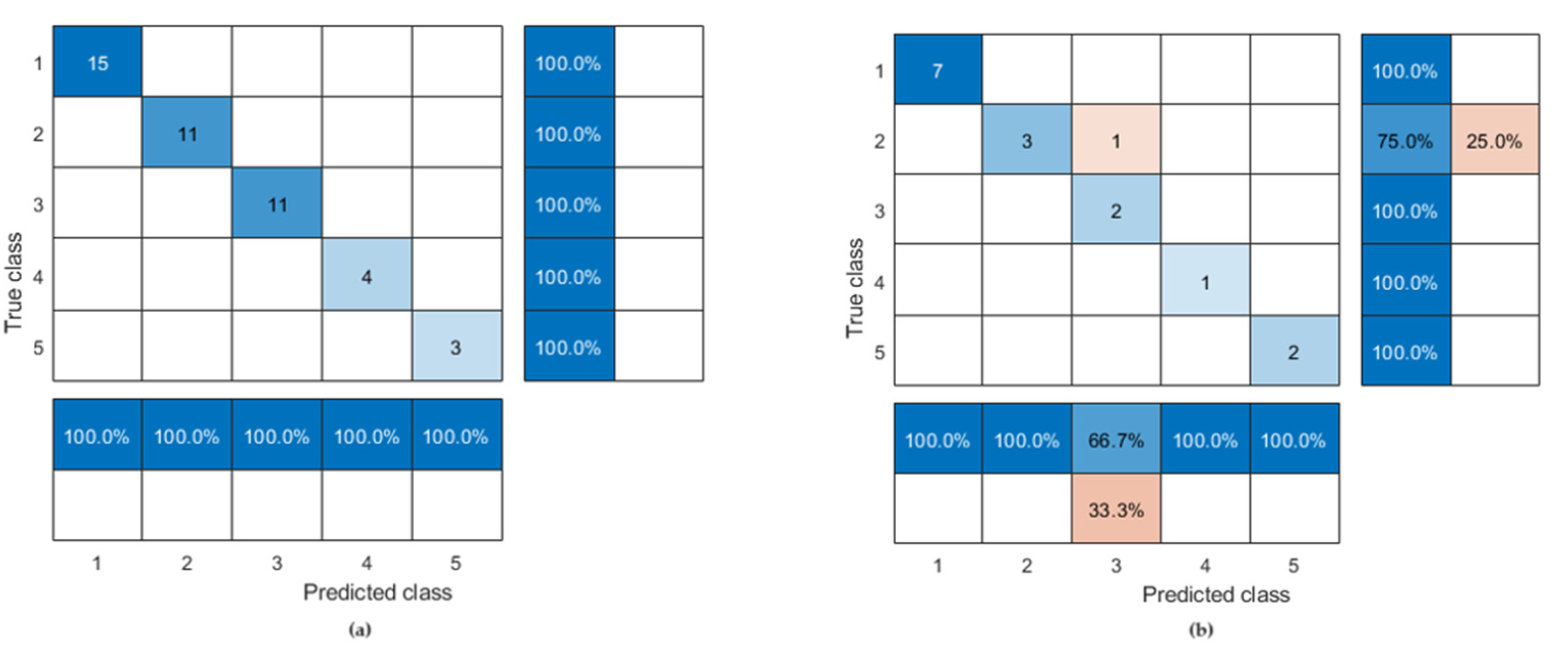
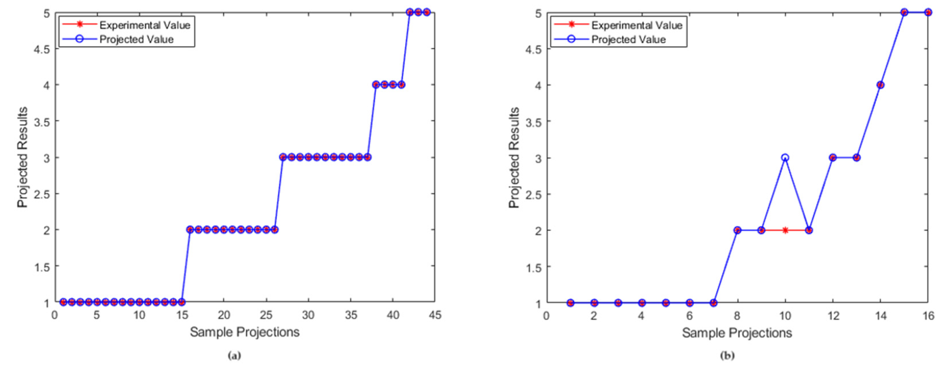
5. Analysis of Projected Results
6. Conclusions
Author Contributions
Funding
Data Availability Statement
Conflicts of Interest
References
- Wu, Y.; Guo, H.; Song, H.; Deng, R. Fuzzy inference system application for oil-water flow patterns identification. Energy 2022, 239, 122359. [Google Scholar] [CrossRef]
- Ohnuki, A.; Akimoto, H. Experimental study on transition of flow pattern and phase distribution in upward air-water two-phase flow along a large vertical pipe. Int. J. Multiph. Flow 2000, 26, 367–386. [Google Scholar] [CrossRef]
- Xu, X.X. Study on oil-water two-phase flow in horizontal pipelines. J. Pet. Sci. Eng. 2007, 59, 43–58. [Google Scholar] [CrossRef]
- Bannwart, A.C.; Rodriguez, O.M.; Trevisan, F.E.; Vieira, F.F.; De Carvalho, C.H. Experimental investigation on liquid-liquid-gas flow: Flow patterns and pressure-gradient. J. Pet. Sci. Eng. 2009, 65, 1–13. [Google Scholar] [CrossRef]
- Su, Q.; Li, J.; Liu, Z. Flow Pattern Identification of Oil–Water Two-Phase Flow Based on SVM Using Ultrasonic Testing Method. Sensors 2022, 22, 6128. [Google Scholar] [CrossRef] [PubMed]
- Trallero, J.L. Oil-Water Flow Patterns in Horizontal Pipes; The University of Tulsa: Tulsa, OK, USA, 1995. [Google Scholar]
- Flores, J.G.; Chen, X.T.; Sarica, C.; Brill, J.P. Characterization of oil-water flow patterns in vertical and deviated wells. SPE Prod. Facil. 1999, 14, 102–109. [Google Scholar] [CrossRef]
- Govier, G.W.; Sullivan, G.A.; Wood, R.K. The upward vertical flow of oil-water mixtures. Can. J. Chem. Eng. 1961, 39, 67–75. [Google Scholar] [CrossRef]
- Yi, X.; Hao, P.; Yi, L.; Wang, H. Flow pattern identification for gas-oil two-phase flow based on a virtual capacitance tomography sensor and numerical simulation. Flow Meas. Instrum. 2023, 92, 102376. [Google Scholar]
- Gao, H.; Gu, H.Y.; Guo, L.J. Numerical study of stratified oil-water two-phase turbulent flow in a horizontal tube. Int. J. Heat Mass Transf. 2003, 46, 749–754. [Google Scholar] [CrossRef]
- Gupta, R.; Fletcher, D.F.; Haynes, B.S. On the CFD modelling of Taylor flow in microchannels. Chem. Eng. Sci. 2009, 64, 2941–2950. [Google Scholar] [CrossRef]
- Etminan, A.; Muzychka, Y.S.; Pope, K. Numerical investigation of gas–liquid and liquid–liquid T aylor flow through a circular microchannel with a sudden expansion. Can. J. Chem. Eng. 2022, 100, 1596–1612. [Google Scholar] [CrossRef]
- Yu, W.; Li, B.; Jia, H.; Zhang, M.; Wang, D. Application of multi-objective genetic algorithm to optimize energy efficiency and thermal comfort in building design. Energy Build. 2015, 88, 135–143. [Google Scholar] [CrossRef]
- Zheng, D.; Qian, Z.D.; Liu, Y.; Liu, C.B. Prediction and sensitivity analysis of long-term skid resistance of epoxy asphalt mixture based on GA-BP neural network. Constr. Build. Mater. 2018, 158, 614–623. [Google Scholar] [CrossRef]
- Hua, S.J.; Sun, Z.R. A novel method of protein secondary structure prediction with high segment overlap measure: Support vector machine approach. J. Mol. Biol. 2001, 308, 397–407. [Google Scholar] [CrossRef] [PubMed]
- Mask, G.; Wu, X.; Ling, K. An improved model for gas-liquid flow pattern prediction based on machine learning. J. Pet. Sci. Eng. 2019, 183, 106370. [Google Scholar] [CrossRef]
- Ambrosio, J.D.S.; Lazzaretti, A.E.; Pipa, D.R.; da Silva, M.J. Two-phase flow pattern classification based on void fraction time series and machine learning. Flow Meas. Instrum. 2022, 83, 102084. [Google Scholar] [CrossRef]
- Alhashem, M. Machine learning classification model for multiphase flow regimes in horizontal pipes. In Proceedings of the International Petroleum Technology Conference, Dhahran, Saudi Arabia, 13–15 January 2020; p. D023S042R001. [Google Scholar]
- Zhou, Y.M.; Wang, S.W.; Lin, L. An Application of BP Neural Network Model to Predict the Moisture Content of Crude Oil. Adv. Mater. Res. 2012, 524–527, 1327–1330. [Google Scholar] [CrossRef]
- Shi, S.; Liu, J.; Hu, H.; Zhou, H. A research on a GA-BP neural network based model for predicting patterns of oil-water two-phase flow in000 horizontal wells. Geoenergy Sci. Eng. 2023, 230, 212151. [Google Scholar] [CrossRef]
- Rokach, L.; Maimon, O. Decision trees. In Data Mining and Knowledge Discovery Handbook; Springer: New York, NY, USA, 2015; pp. 165–192. [Google Scholar]
- Breiman, L.; Friedman, J.; Olshen, R.; Stone, C. Classification and Regression Trees; Wadsworth Int. Group: Belmont, CA, USA, 1984; Volume 37, pp. 237–251. [Google Scholar]
- Quinlan, J.R. C4. 5: Programs for Machine Learning; Elsevier: Amsterdam, The Netherlands, 2014. [Google Scholar]
- Shafer, J.C.; Agrawal, R.; Mehta, M. A scalable parallel classi er for data mining. In Proceedings of the 22nd International Conference on VLDB, Mumbai, India, 3–6 September 1996. [Google Scholar]
- Mehta, M.; Agrawal, R.; Rissanen, J. SLIQ: A fast scalable classifier for data mining. In Advances in Database Technology—EDBT’96: 5th International Conference on Extending Database Technology Avignon, France, 25–29 March 1996 Proceedings 5; Springer: Berlin/Heidelberg, Germany, 1996; pp. 18–32. [Google Scholar]
- Wang, S.M.; Zhou, J.; Li, C.Q.; Armaghani, D.J.; Li, X.B.; Mitri, H.S. Rockburst prediction in hard rock mines developing bagging and boosting tree-based ensemble techniques. J. Cent. S. Univ. 2021, 28, 527–542. [Google Scholar] [CrossRef]
- Breiman, L. Random forests. Mach. Learn. 2001, 45, 5–32. [Google Scholar] [CrossRef]


| Density (g/cm3) | Viscosity (mPa·s) | |
|---|---|---|
| Oil | 0.826 | 2.92 |
| Water | 0.988 | 1.16 |
| Flow Pattern | Coding |
|---|---|
| bubble flow | 1 |
| emulsion flow | 2 |
| froth flow | 3 |
| wavy flow | 4 |
| stratified flow | 5 |
| Water Cut (%) | Angle of Inclination (°) | Flow Rate (m3/d) | Experimental Flow Pattern | GA-BP | Accuracy Rate | Random Forest | Accuracy Rate |
|---|---|---|---|---|---|---|---|
| 20 | 0 | 100 | 1 | 1 | 81.25% | 1 | 93.75% |
| 85 | 600 | 2 | 2 | 2 | |||
| 85 | 100 | 4 | 4 | 4 | |||
| 90 | 600 | 2 | 2 | 2 | |||
| 40 | 60 | 100 | 1 | 1 | 1 | ||
| 85 | 300 | 1 | 1 | 1 | |||
| 90 | 100 | 5 | 5 | 5 | |||
| 90 | 600 | 3 | 3 | 3 | |||
| 60 | 0 | 600 | 2 | 3 | 3 | ||
| 60 | 100 | 1 | 1 | 1 | |||
| 60 | 600 | 2 | 3 | 2 | |||
| 80 | 0 | 100 | 1 | 1 | 1 | ||
| 90 | 0 | 100 | 1 | 1 | 1 | ||
| 90 | 100 | 5 | 4 | 5 | |||
| 90 | 300 | 1 | 1 | 1 | |||
| 90 | 600 | 3 | 3 | 3 |
| Experimental Flow Patterns | Actual Flow Pattern | GA-BP Predictive Flow Patterns | Random Forest Predictive Flow Patterns |
|---|---|---|---|
 | Emulsion flow | Froth flow | Froth flow |
 | Emulsion flow | Froth flow | Emulsion flow |
 | Stratified flow | Wavy flow | Stratified flow |
Disclaimer/Publisher’s Note: The statements, opinions and data contained in all publications are solely those of the individual author(s) and contributor(s) and not of MDPI and/or the editor(s). MDPI and/or the editor(s) disclaim responsibility for any injury to people or property resulting from any ideas, methods, instructions or products referred to in the content. |
© 2023 by the authors. Licensee MDPI, Basel, Switzerland. This article is an open access article distributed under the terms and conditions of the Creative Commons Attribution (CC BY) license (https://creativecommons.org/licenses/by/4.0/).
Share and Cite
Sun, Y.; Guo, H.; Liang, H.; Li, A.; Zhang, Y.; Zhang, D. A Comparative Study of Oil–Water Two-Phase Flow Pattern Prediction Based on the GA-BP Neural Network and Random Forest Algorithm. Processes 2023, 11, 3155. https://doi.org/10.3390/pr11113155
Sun Y, Guo H, Liang H, Li A, Zhang Y, Zhang D. A Comparative Study of Oil–Water Two-Phase Flow Pattern Prediction Based on the GA-BP Neural Network and Random Forest Algorithm. Processes. 2023; 11(11):3155. https://doi.org/10.3390/pr11113155
Chicago/Turabian StyleSun, Yongtuo, Haimin Guo, Haoxun Liang, Ao Li, Yiran Zhang, and Doujuan Zhang. 2023. "A Comparative Study of Oil–Water Two-Phase Flow Pattern Prediction Based on the GA-BP Neural Network and Random Forest Algorithm" Processes 11, no. 11: 3155. https://doi.org/10.3390/pr11113155
APA StyleSun, Y., Guo, H., Liang, H., Li, A., Zhang, Y., & Zhang, D. (2023). A Comparative Study of Oil–Water Two-Phase Flow Pattern Prediction Based on the GA-BP Neural Network and Random Forest Algorithm. Processes, 11(11), 3155. https://doi.org/10.3390/pr11113155