Article

Reservoir Petrofacies Predicted Using Logs Data: A Study of Shale Oil from Seven Members of the Upper Triassic Yanchang Formation, Ordos Basin, China

1
State Key Laboratory of Continental Dynamics, Department of Geology, Northwest University, Xi’an 710069, China
2
Research Institute of Petroleum Exploration and Development, SINOPEC, Beijing 100083, China
3
Research Institute of Exploration & Development, Changqing Oilfield, PetroChina, Xi’an 710018, China
4
Exploration and Development Research Institute, Shengli Oilfield Company, SINOPEC, Dongying 257015, China
5
School of Petroleum Engineering, Xi’an Shiyou University, Xi’an 257015, China
*
Author to whom correspondence should be addressed.
Processes 2023, 11(11), 3131; https://doi.org/10.3390/pr11113131
Submission received: 13 September 2023 / Revised: 14 October 2023 / Accepted: 18 October 2023 / Published: 1 November 2023

Abstract

:
The identification and prediction of petrofacies plays a crucial role in the study of shale oil and gas “sweet spots”. However, the petrofacies identified through core and core test data are not available for all wells. Therefore, it is essential to establish a petrofacies identification model using conventional well logging data. In this study, we determined the petrofacies of shale oil reservoirs in the Upper Triassic Yanchang Formation, Ordos Basin, China, based on scanning electron microscopy, core porosity and total organic carbon (TOC), and brittleness index calculations from X-ray diffraction (XRD) experiments conducted on seven members of the formation. Furthermore, we compared the interpreted logs with the raw well logs data clustered into electrofacies in order to assess their compliance with the petrofacies, using the Multi-Resolution Graph-Based Clustering (MRGC) method. Through an analysis of pore structure type, core porosity, TOC, and brittleness index, we identified four types of lithofacies with varying reservoir quality: PF A > PF B > PF C > PF D. The compliance of the clustered electrofacies with the petrofacies obtained from the interpreted logs was found to be 85.42%. However, the compliance between the clustered electrofacies and the petrofacies obtained from the raw well logs was only 47.92%. Hence, the interpreted logs exhibit a stronger correlation with petrofacies characterization, and their utilization as input data is more beneficial in accurately predicting petrofacies through machine learning algorithms.

1. Introduction

Lake-phase mudstone, shale, and oil shale, along with other fine-grained sedimentary rocks, are abundant in the Triassic Yanchang Formation of the Ordos Basin, offering significant potential for unconventional oil and gas resources such as shale oil and gas and oil shale [1]. The classification of reservoir petrofacies serves as the foundation and key to oil and gas exploration, with facies exerting a significant control on the distribution of shale oil and gas. Therefore, it holds immense importance to accurately characterize and predict reservoir petrofacies [2,3]. Petrofacies studies typically rely on core data, encompassing observations of core hand specimens, thin sections, scanning electron microscopy, X-ray diffraction (XRD), and physical property tests [4,5,6,7]. However, the availability of cores is often limited due to constraints in drilling time and cost [3,8]. Geophysical logging data, on the other hand, contain rich petrophysical information, enabling indirect petrofacies classification. Nevertheless, given the complexity and heterogeneity of the reservoir, there exists a considerable amount of redundancy among the log curves, necessitating careful selection of curve attributes and algorithm preferences for accurate petrofacies prediction [5,9,10,11].
The classification of shale petrofacies typically relies on indicators such as hydrocarbon-bearing fracturability, organic matter abundance, sedimentary structure, and mineralogical fractions, which are crucial in assessing their potential for hydrocarbon production [12,13,14]. Venieri et al. (2021) classified organic-rich shales into five lithofacies categories based on core observations, X-ray diffraction (XRD) analyses, and log response characterization [15]. Atchley et al. (2021) classified shale reservoirs into six petrofacies based on gamma ray measurements, density porosity cut-offs, and total organic carbon (TOC) values [14]. Consequently, petrofacies often exhibit distinct characteristics in logging curves, forming the basis for petrofacies prediction through logging data. Currently, many scholars have achieved satisfactory results in petrofacies identification using machine learning algorithms [11,16,17]. In machine learning, facies prediction is typically accomplished through clustering or classification algorithms [18,19]. Clustering algorithms are straightforward, as they do not require prior knowledge regarding the number and attributes of facies, nor do they require training [9]. Among these clustering algorithms, the Multi-Resolution Graph-Based Clustering (MRGC) algorithm has proven successful in log curve reconstruction [20], permeability prediction [21], flow zone unit determination [22], and petrofacies identification [5,23,24].
The shale of the seventh member of the Triassic Yanchang Formation is widely distributed, and it serves as a significant hydrocarbon source rock with substantial resources. At the Ordos Basin, the estimated resource amount reaches 33 × 108 metric tons [25]. In this study, the petrofacies type of the shale oil interval was determined through various methods, including scanning electron microscopy (SEM), core porosity and total organic carbon (TOC) analysis, and X-ray diffraction (XRD) experiments. Furthermore, we assessed the consistency between the electrofacies and the petrofacies derived from interpreted logs and raw well logs, which were clustered and used as input data in conjunction with the MRGC algorithm. Our findings contribute to the development of petrofacies classification schemes for shale reservoirs and provide a viable approach for high-precision petrofacies prediction.

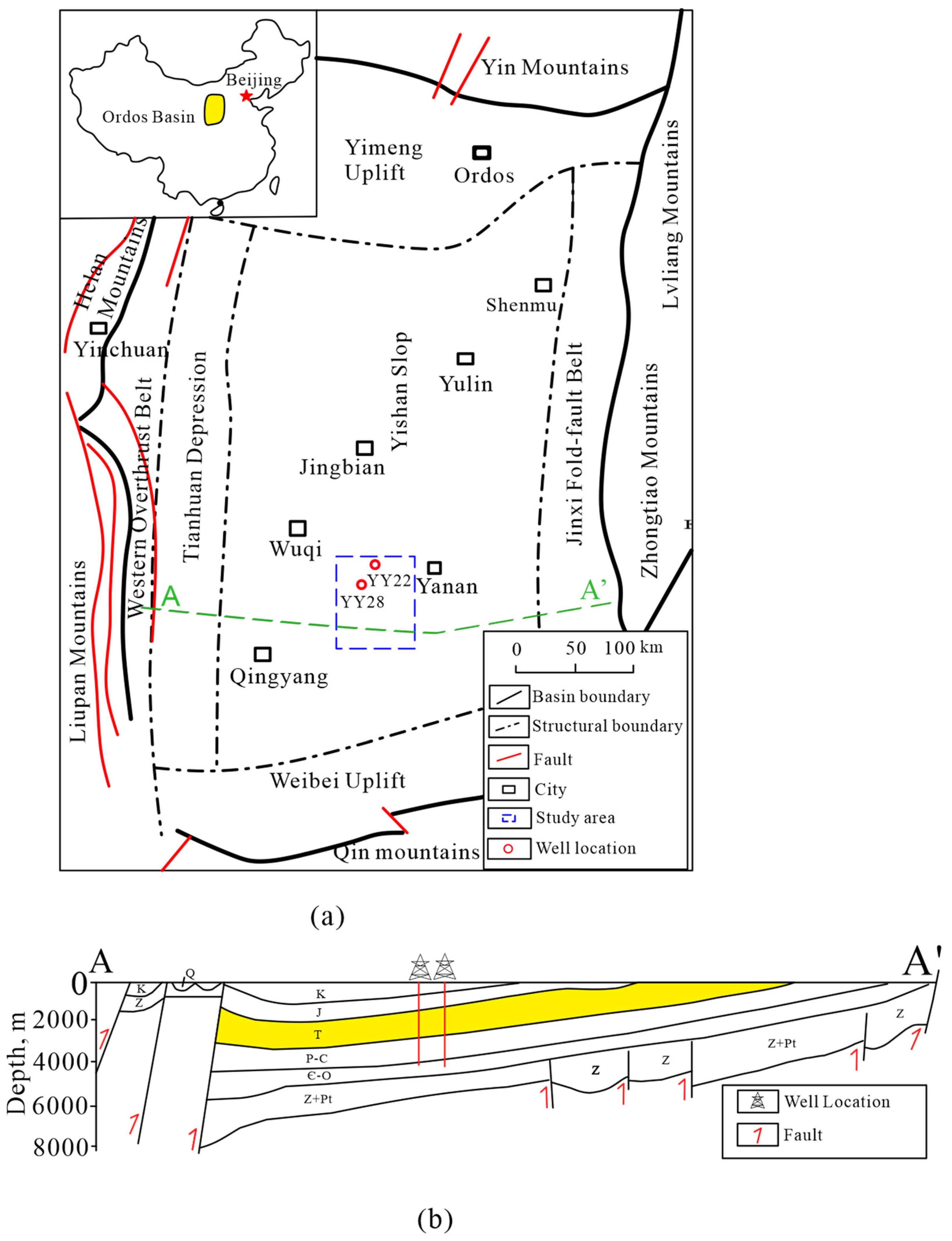
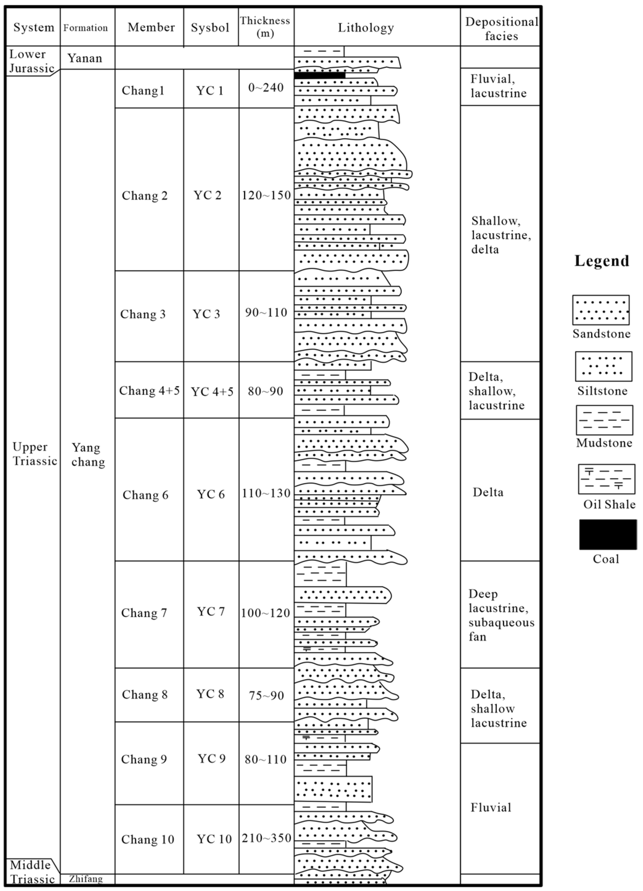
2. Geological Background

The Ordos Basin, located in the western part of the North China Platform, is the second largest sedimentary basin in China. It can be divided into six major tectonic units: the Yimeng Uplift, Weibei Uplift, Western Overthrust Belt, Tianhuan Depression, Yishan Slope, and Jinxi Fold-Fault Belt (Figure 1a). This basin originated on the stable crystalline basement of the Taikonian period and experienced tectonic sedimentary infill evolution from the Paleozoic to the Cenozoic, resulting in the formation of a cover layer with an average thickness of 4–5 km [26]. During the Late Triassic, the southern part of the basin underwent uplift due to the collision between the Yangzi Plate and the North China Plate, serving as the primary source of material for the southern region of the basin [27]. The North China Plate experienced extrusion from the south by the offset of the Yangzi Plate and from the north by the Xingmeng Plate, causing subsidence and forming a slope with angles of 3.5° to 5.5° in the south and 1.5° to 2.5° in the north of the Late Triassic Basin, respectively [26,28]. In the early Late Triassic, the basin’s basement rapidly subsided, leading to the intrusion of lakes and the transportation and accumulation of sediments from the Qinling and Liupanshan regions in the south and the Yinshan Mountains in the north, respectively [26,29].
Our study area is located in the southern part of the Ordos Basin (Figure 1a), and several drilled hydrocarbon wells in the region encounter Triassic formations (Figure 1b). The Upper Triassic Yanchang Formation is stratigraphically divided into 10 sublayers, ranging from YC10 to YC1 (Figure 2). The YC7 reservoir is identified as an unconventional shale reservoir, with a thickness between 100 and 120 m. The lithology is predominantly dark black mud shale interbedded with thin layers of silty mudstone and silty siltstone. During the deposition of the YC7, the lake basin experienced significant tectonic activity and underwent rapid expansion, ultimately becoming the largest lake in the Mesozoic era within the Ordos Basin [32]. The lake-phase mudstone and shale extend in a northwest–southeast direction across the region, corresponding to the semi-deep to deep lake zone. The thickness of these shale deposits ranges from 10 to 120 m, with some areas exhibiting shale layers exceeding 10 m in thickness over an extent of up to 3 × 10⁴ square kilometers [33].

3. Materials and Methods

3.1. Materials and Experiments

Conventional logging data and ECS logging data were collected from two wells in the study area. The locations of the two wells are displayed in Figure 1. The conventional logging data comprise CAL (Caliper), SP (Spontaneous Potential), GR (Gamma ray), PE (Photoelectric Absorption Cross-Section Index), DT (Compressional Slowness), NPHI (Neutron Porosity), DEN (Bulk Density), RD (Deep Resistivity), and RS (Shallow Resistivity).
A total of 48 depth points were sampled to collect core samples for experimental analysis. Porosity measurements were conducted using an ULTRAPORE-200A helium core porosimeter (Core Lab, USA) at a temperature of 25 °C and pressure of 1.025 bar. To determine the total organic carbon (TOC) content in the shale samples, pyrolysis experiments were performed using the Rock-Eval 6 analyzer. The experimental results for core porosity and TOC are summarized in Table 1. X-ray diffraction (XRD) experiments were conducted on the shale samples to analyze the mineral fractions. A MiniFlex 600 instrument equipped with Cu-Kα radiation was used, and the experimental samples were 300 mesh powders. The XRD analysis involved scanning the samples from 5° to 90° in 0.02° increments to obtain precise and accurate results [35]. The microstructure of the samples was examined using scanning electron microscopy, and the corresponding results are presented in Table 2.

3.2. The Multi-Resolution Graph-Based Clustering (MRGC) Algorithms

The MRGC algorithm is an unsupervised clustering algorithm that combines the advantages of the KNN (K-Nearest Neighbors) algorithm and graph theory algorithm [36]. Two important parameters in this algorithm are the neighbor index (NI) and the kernel representative index (KRI). In the context of considering the sample set as an attraction set with an attraction relationship, the NI represents the ability of a sample point to attract all other sample points within the attraction set. A higher NI value indicates that the point is closer to the core of a class [20]. On the other hand, the KRI reflects the ability of the current attraction set to act as a kernel for fusing other attraction sets. A higher KRI value signifies that the attraction set has a greater dominance in the fusion process [37].
Let’s assume that there are N sample points in the sample set S to be classified, denoted as S = { x 1, x 2, …, x i, …, x N}. Each sample point x in the sample set S is represented as a vector with multiple attributes, and y represents the nth closest sample point to x in the sample set S, where nN − 1. In order to determine the point at which no further attraction exists between sample points, a threshold K is set, indicating the Kth nearest neighbor. The attractiveness of a sample point x towards its nth sample point can be mathematically expressed as follows:
δ n x = e m α , x   i s   t h e   m t h   n e a r e s t   n e i g h b o r   s a m p l e   p o i n t   o f   y , m K       0   ,     x   d o e s   n o t   b e l o n g   t o   t h e   s e t   o f   K   n e a r e s t   n e i g h b o r s   o f   y
where α represents the smoothing factor greater than zero [23]. For each sample point in the set, the following calculations are performed:
S x = i = 1 N 1 δ n x
The neighbor index of a sample point x is determined by the normalized value of the S x function and can be mathematically expressed as follows:
N I x = S x S m i n S m a x S m i n
Among them,
S m i n = M i n S x i i = 1,2 , , N
S m a x = M a x S x i i = 1,2 , , N
S m i n and S m a x are the minimum and maximum values of the S x function, respectively; N I x lies between 0 and 1.
The values S m i n and S m a x represent the minimum and maximum values of the S x function, respectively. The neighbor index N I x is a normalized value that falls within the range of 0 and 1.
The neighbor index (NI) is a localized index derived from the kernel representative index (KRI) that incorporates both the neighbor index of the current sample point and the neighboring relationships and spatial distances of the sample points. The KRI can be mathematically expressed as follows:
K R I x = M x , z × N I x × D x , z
where z represents the nearest neighbor sample points to the sample point x based on the proximity index. M( x , z) denotes the neighborhood number of the sample point x relative to the sample z. D( x , z) represents the distance function, commonly calculated using the Euclidean distance formula.
The kernel representative index (KRI) is sorted in descending order to create a curve, which exhibits multiple inflection points that mark the transition from one smooth segment to another. Each inflection point indicates a change in the classification level, representing different levels of clustering results [24]. Based on specific facies analysis requirements, users have the flexibility to set parameters such as the maximum number of clusters, the minimum number of clusters, and the maximum number of optimal clustering schemes. Through analysis and calculation, the MRGC algorithm can automatically identify and compare several optimal clustering schemes, enabling users to efficiently delineate electrofacies [5,23].

4. Results

4.1. Petrofacies

The total organic carbon (TOC) content, reservoir properties, and fracturability play crucial roles in the development of shale oil and gas reservoirs. In this study, a total of 48 core samples were collected to analyze porosity, TOC content, and mineral fractions. In a related study by Kang et al. (2020), a novel mineralogical brittleness index was introduced, which considers the presence of brittle minerals in shale formations [38]. The mineralogical brittleness index can be mathematically defined as a function of the weights of brittle minerals:
B I b m = W Q + 0.49 × W F + 0.51 × W c + 0.44 × W D / W T
where W Q , W F , W c , and W D represent the weights percentage of quartz, feldspar, calcite, and dolomite, respectively. Additionally, W T denotes the total mineral weight percentage (=100%). The brittleness index was calculated for the mineral fractions obtained through experimental analysis. The results of the brittleness index calculations are summarized in Table 1.
The “sweet spot” criteria for a shale reservoir typically involve high porosity, total organic carbon (TOC) content, and brittleness index [15,39,40]. In this study, we examined the correlation between core TOC, porosity (POR), and the mineralogical brittleness index (BIbm). TOC and POR showed a positive correlation based on the distribution of most points (Figure 3a). TOC and BIbm showed a negative correlation based on the distribution of most points (Figure 3c). There was little correlation between POR and BIbm (Figure 3b). For the “sweet spot” of shale oil reservoirs, we prefer reservoirs with high POR, high TOC, and high brittleness index. Consequently, the petrofacies classification necessitates a trade-off between BIbm and TOC.
Based on SEM, core porosity, TOC, and brittleness index, we classified petrofacies into four types (Table 2).
Petrofacies A: High porosity (1.48–4.70%, average 2.17%), high TOC (2.29–15.19%, average 6.35%), and high BIbm (25.77–38.95%, average 32.87%). Clay mineral interlayer pores, fractures, and interparticle pores are developed.
Petrofacies B: Median porosity (1.34–3.90%, average 2.01%), median TOC (2.89–8.03%, average 5.04%), and high BIbm (23.33–38.17%, average 29.76%). Intraparticle pores and interparticle pores are developed.
Petrofacies C: Low porosity (0.80–2.62%, average 1.61%), median TOC (3.16–7.26%, average 5.10%), and low BIbm (10.25–29.87%, average 24.78%). Clay mineral interlayer pores and fractures are developed; interparticle and intraparticle pores are sparsely developed.
Petrofacies D: Ultra-low porosity (0.50–1.44%, average 1.01%), low TOC (0.48–9.93%, average 4.17%), and high BIbm (17.12–50.67%, average 30.29%). Clay mineral interlayer pores and fractures are developed.

4.2. Electrofacies

We performed electrofacies analysis by the MRGC algorithm using two types of logging data: one with interpreted logs (Model 1) and the other with raw well logs (Model 2). We compared the predictive effectiveness of both models.

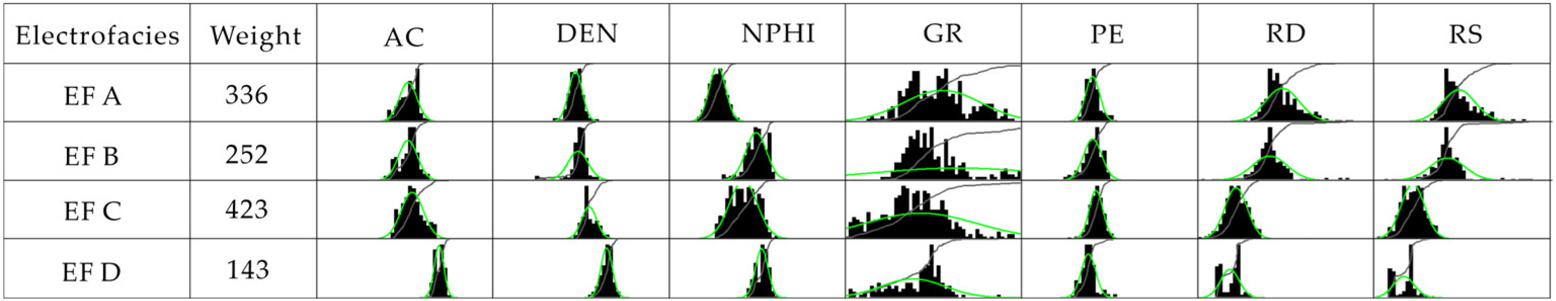
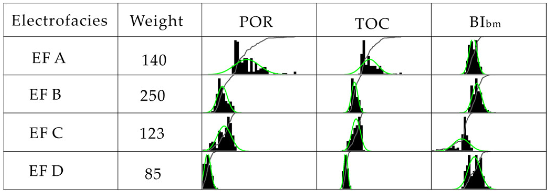
4.2.1. Electrofacies from Interpreted Logs

POR and TOC were interpreted using conventional logging using the method proposed by Yu et al. (2017, 2018) [39,40]. The brittleness index was calculated using ECS logging, using the method proposed by Kang et al. (2020) [38]. Interpreted logs (POR, TOC, and BI) were used as input data for clustering to obtain electrofacies via the MRGC algorithm. Interpreted logs ultimately classify electrofacies into four types (Figure 4). EF A: high porosity, high TOC, and high brittleness index; EF B: median porosity, median TOC, and high brittleness index; EF C: median porosity, median TOC, and low brittleness index; EF D: tight porosity, low TOC, and high brittleness index. The electrofacies types obtained by clustering have more consistent characteristics with petrofacies types.
Electrofacies clustering results for tight oil reservoirs from two wells are presented in log plots (Figure 5). The 10th track shows petrofacies obtained by core SEM, core porosity, core TOC, and brittleness index calculated from XRD. The 11th track shows the classification results of electrofacies from the interpreted logs data using the MRGC algorithm (Model 1). The core-based petrofacies are in agreement with the model 1 electrofacies. The electrofacies obtained from model 1 clustering are 85.42% compatible with the core-based petrofacies.

4.2.2. Electrofacies from Raw Well Logs

Electrofacies are often clustered using conventional logging data [5,41]. The conventional log data selected for this study include AC, DEN, NPHI, GR, PE, RD, and RS. Raw well logs were used as input data for clustering to obtain electrofacies via the MRGC algorithm. Raw well logs ultimately classify electrofacies into four types (Figure 6). EF A: low AC, low DEN, low NPHI, high GR, high PE, high RD, and high RS; EF B: low AC, low DEN, high NPHI, high GR, high PE, median RD, and median RS; EF C: low AC, median DEN, median NPHI, low GR, high PE, low RD, and low RS; EF D: high AC, high DEN, high NPHI, low GR, low PE, low RD, and low RS. Raw well logs curves indirectly respond to the properties of the reservoir.
Electrofacies clustering results for tight oil reservoirs from two wells are presented in log plots (Figure 5). The 12th track shows the classification results of electrofacies from the raw well logs data using the MRGC algorithm (Model 2). Electrofacies are characterized by homogeneity at successive depths and show weak sensitivity to petrofacies changes. The core-based petrofacies are in poor agreement with the model 2 electrofacies. The electrofacies obtained from model 2 clustering are 47.92% compatible with the core-based petrofacies.

5. Discussion

This paper classifies petrofacies of shale oil reservoirs based on SEM, core porosity, core TOC, and mineralogy of brittleness index calculated from XRD experiments from seven members of the Upper Triassic Yanchang Formation, Ordos Basin, China. Petrofacies are initially defined as “intervals of rock with a similar average pore throat radius, thus having similar fluid flow characteristics” [42,43]. Many authors also define petrography based on a combination of core analysis characteristics, petrographic features (grain size, sorting, mineralogy, and pore type), and well logging characteristics [2,44,45]. Our petrofacies classification scheme focuses on four key criteria of shale reservoirs: porosity and pore types determine the reservoir’s storage performance and fluid endowment state [46,47], TOC determines the reservoir’s hydrocarbon potential [48,49], and brittleness index determines the reservoir’s remodeling ability [50,51,52]. Venier et al. identified five petrofacies through core hand specimens, mineralogical composition obtained from XRD experiments, TOC, and logging responses [15]. We consider the mineralogical brittleness index obtained from XRD experiments to be a more direct criterion for the classification of petrofacies.
We used interpreted logs and raw well logs as input data to obtain four types of electrofacies by clustering with the MRGC algorithm and established the mapping relationship with petrofacies. Further comparisons were made between the performance of the two types of data modeling for petrofacies prediction. MRGC is one of the few non-parametric methods that is well suited for the learning and clustering of analyzed data from logs and drilled cores [5]. Many scholars have modeled the identification of facies using logging data via the MRGC algorithm [5,20,53,54]. The properties of the interpreted logs are more closely related to the characteristics of the petrofacies, and the raw well logs contain redundant signals that can only indirectly reflect the characteristics of the petrofacies. A limited set of good input datasets is better than a larger set of attribute input datasets, as it reduces data redundancy and improves clustering efficiency [9]. Analyses of the available data confirmed this conclusion. The number of interpreted logs is low but more closely related to petrofacies. Therefore, model 1 based on interpreted logs as the input has a higher accuracy for the identification of petrofacies compared to model 2 based on raw well logs as the input (Figure 5).

6. Conclusions

Petrofacies are an important tool that represents different reservoir qualities [2] and can be modeled for logging identification [9]. In this study, we classified the shale oil reservoir into four petrofacies based on the shale’s pore structure, porosity, TOC, and brittleness index through experimental data from the seven members of the Upper Triassic Yanchang Formation, Ordos Basin, China. PF A is characterized by optimal reservoir properties and has good reservoir performance, hydrocarbon potential, and fracturability. PF B is inferior to PF A in terms of reservoir performance and hydrocarbon potential. PF C has a poor brittleness index, making it unsuitable for fracture modification. PF D cannot be used as an effective reservoir.
Interpreted logs and raw well logs data were used as input clustering to obtain electrofacies using the MRGC algorithm. The clustered electrofacies of the raw logging data showed poor sensitivity to changes in petrofacies. In contrast, the clustered electrofacies from the interpreted logs matched the petrofacies more closely. Therefore, extracting interpreted logs related to petrofacies from conventional logs is necessary to improve the accuracy of petrofacies prediction.

Author Contributions

Conceptualization, K.M. and H.Y.; methodology, K.M. and M.W; software, Y.J. and C.M.; validation, S.Z. and H.Y.; investigation, S.Z. and Y.J.; data curation, M.W.; writing—original draft preparation, K.M. and P.X.; writing—review and editing, M.W., J.Z. and H.Y.; visualization, K.M. and P.X.; supervision, H.Y., J.Z. and M.W. All authors have read and agreed to the published version of the manuscript.

Funding

This work was jointly funded by the Natural Science Basic Research Plan in Shaanxi Province of China (2020JQ-594), the Young Talent fund of the University Association for Science and Technology in Shaanxi, China (20180701), the Major Science and Technology Project of Changqing Oilfield Company, PetroChina (ZDZX2021-03; ZDZX2021-05), Northwest University “Zhongying Young Scholars” Support Project and Aeronautical Science Foundation of China (2018ZE53052).

Data Availability Statement

The data presented in this study are available on request from the corresponding author. The data are not publicly available due to restrictions of privacy.

Acknowledgments

The authors thank the reviewers for their valuable comments and are grateful to the editor for careful editing.

Conflicts of Interest

The authors declare no conflict of interest.

References

  1. Yang, R.; Yin, W.; Fan, A.; Han, Z. Fine-Grained, Lacustrine Gravity-Flow Deposits and Their Hydrocarbon Significance in the Triassic Yanchang Formation in Southern Ordos Basin. J. Palaeogeogr. 2017, 19, 791–806, (In Chinese, with English Abstract). [Google Scholar] [CrossRef]
  2. Cao, B.; Sun, W.; Li, J. Reservoir Petrofacies—A Tool for Characterization of Reservoir Quality and Pore Structures in a Tight Sandstone Reservoir: A Study from the Sixth Member of Upper Triassic Yanchang Formation, Ordos Basin, China. J. Pet. Sci. Eng. 2021, 199, 108294. [Google Scholar] [CrossRef]
  3. Cao, B.; Luo, X.; Zhang, L.; Lei, Y.; Zhou, J. Petrofacies Prediction and 3-D Geological Model in Tight Gas Sandstone Reservoirs by Integration of Well Logs and Geostatistical Modeling. Mar. Pet. Geol. 2020, 114, 104202. [Google Scholar] [CrossRef]
  4. Li, B.; Pang, X.; Dong, Y.; Peng, J.; Gao, P.; Wu, H.; Huang, C.; Shao, X. Lithofacies and Pore Characterization in an Argillaceous-Siliceous-Calcareous Shale System: A Case Study of the Shahejie Formation in Nanpu Sag, Bohai Bay Basin, China. J. Pet. Sci. Eng. 2019, 173, 804–819. [Google Scholar] [CrossRef]
  5. Jafarzadeh, N.; Kadkhodaie, A.; Ahmad, B.J.; Kadkhodaie, R.; Karimi, M. Identification of Electrical and Petrophysical Rock Types Based on Core and Well Logs: Utilizing the Results to Delineate Prolific Zones in Deep Water Sandy Packages from the Shah Deniz Gas Field in the South Caspian Sea Basin. J. Nat. Gas Sci. Eng. 2019, 69, 102923. [Google Scholar] [CrossRef]
  6. Ros De, L.F.; Goldberg, K. Reservoir Petrofacies: A Tool for Quality Characterization and Predictions. In Proceedings of the AAPG Annual Convention, Long Beach, CA, USA, 1–4 April 2007. [Google Scholar]
  7. Trop, T.M.; Ridgway, K.D. Petrofacies and Provenance of a Late Cretaceous Suture Zone Thrust-Top Basin, Cantwell Basin, Central Alaska Range. J. Sediment. Res. 1997, 67, 469–485. [Google Scholar]
  8. Silva, A.; Tavares, M.; Carrasquilla, A.; Missagia, R.; Ceia, M. Petrofacies Classification Using Machine Learning Algorithms. Geophysics 2020, 85, WA101–WA113. [Google Scholar] [CrossRef]
  9. Glover, P.W.J.; Mohammed-Sajed, O.K.; Akyüz, C.; Lorinczi, P.; Collier, R. Clustering of Facies in Tight Carbonates Using Machine Learning. Mar. Pet. Geol. 2022, 144, 105828. [Google Scholar] [CrossRef]
  10. Wang, M.; Yang, J.; Wang, X.; Li, J.; Xu, L.; Yan, Y. Identification of Shale Lithofacies by Well Logs Based on Random Forest Algorithm. Earth Sci. 2023, 48, 130–142. [Google Scholar] [CrossRef]
  11. Al-Mudhafar, W.J. Integrating Component Analysis & Classification Techniques for Comparative Prediction of Continuous & Discrete Lithofacies Distributions. In Proceedings of the Offshore Technology Conference, Houston, TX, USA, 2–5 May 2015; p. OTC-25806-MS. [Google Scholar]
  12. Liu, B.; Shi, J.; Fu, X.; Lyu, Y.; Sun, X.; Gong, L.; Bai, Y. Petrological Characteristics and Shale Oil Enrichment of Lacustrine Fine-Grained Sedimentary System: A Case Study of Organic-Rich Shale in First Member of Cretaceous Qingshankou Formation in Gulong Sag, Songliao Basin, NE China. Pet. Explor. Dev. 2018, 45, 884–894. [Google Scholar] [CrossRef]
  13. Wang, G.; Carr, T. Organic-Rich Marcellus Shale Lithofacies Modeling and Distribution Pattern Analysis in the Appalachian Basin. AAPG Bull. 2013, 97, 2173–2205. [Google Scholar] [CrossRef]
  14. Atchley, S.; Crass, B.; Prince, K. The Prediction of Organic-Rich Reservoir Facies within the Late Pennsylvanian Cline Shale (Also Known as Wolfcamp D), Midland Basin, Texas. AAPG Bull. 2021, 105, 29–52. [Google Scholar] [CrossRef]
  15. Venieri, M.; Harazim, D.; Pedersen, P.K.; Eaton, D.W. Vertical and Lateral Facies Variability in Organic-Rich Mudstones at the Reservoir Scale: A Case Study from the Devonian Duvernay Formation of Alberta, Canada. Mar. Pet. Geol. 2021, 132, 105232. [Google Scholar] [CrossRef]
  16. Gifford, C.M.; Agah, A. Collaborative Multi-Agent Rock Facies Classification from Wireline Well Log Data. Eng. Appl. Artif. Intell. 2010, 23, 1158–1172. [Google Scholar] [CrossRef]
  17. Al-Mudhafar, W.J.; Al Lawe, E.M.; Noshi, C.I. Clustering Analysis for Improved Characterization of Carbonate Reservoirs in a Southern Iraqi Oil Field; OnePetro: Richardson, TX, USA, 2019. [Google Scholar]
  18. Witten, I.H.; Frank, E.; Hall, H. Data Mining: Practical Machine Learning Tools and Techniques; Morgan Kaufmann: New Brunswick, NJ, USA, 2011; ISBN 978-0-12-374856-0. [Google Scholar]
  19. Han, R.; Wang, Z.; Guo, Y.; Wang, X.; A, R.; Zhong, G. Multi-Label Prediction Method for Lithology, Lithofacies and Fluid Classes Based on Data Augmentation by Cascade Forest. Adv. Geo-Energy Res. 2023, 9, 25–37. [Google Scholar] [CrossRef]
  20. Pabakhsh, M.; Ahmadi, K.; Riahi, M.A.; Shahri, A.A. Prediction of PEF and LITH Logs Using MRGC Approach. Life Sci. J. 2012, 9, 974–982. [Google Scholar]
  21. Khoshbakht, F.; Mohammadnia, M. Assessment of Clustering Methods for Predicting Permeability in a Heterogeneous Carbonate Reservoir. In Proceedings of the 4th International Conference and Exhibition: New Discoveries through Integration of Geosciences, Saint Petersburg, Russia, 5–8 April 2010. [Google Scholar] [CrossRef]
  22. Nouri-Taleghani, M.; Kadkhodaie, A.; Karimi-Khaledi, M. Determining Hydraulic Flow Units Using a Hybrid Neural Network and Multi-Resolution Graph-Based Clustering Method: Case Study from South Pars Gasfield, Iran. J. Pet. Geol. 2015, 38, 177–191. [Google Scholar] [CrossRef]
  23. Tian, Y.; Xu, H.; Zhang, X.-Y.; Wang, H.-J.; Guo, T.-C.; Zhang, L.-J.; Gong, X.-L. Multi-Resolution Graph-Based Clustering Analysis for Lithofacies Identification from Well Log Data: Case Study of Intraplatform Bank Gas Fields, Amu Darya Basin. Appl. Geophys. 2016, 13, 598–607. [Google Scholar] [CrossRef]
  24. Sutadiwiria, Y. Using MRGC (Multi-Resolution Graph-Based Clustering) Method to Integrate Log Data and Core Facies to Diffine Electrofacies, in the Benua Field, Central Sumatera Basin, Indonesia. In Proceedings of the International Gas Union Research Conference, Paris, France, 8–10 October 2008; pp. 733–744. [Google Scholar]
  25. Zhao, W.; Hu, S.; Hou, L.; Yang, T.; Li, X.; Guo, B.; Yang, Z. Types and Resource Potential of Continental Shale Oil in China and Its Boundary with Tight Oil. Pet. Explor. Dev. 2020, 47, 1–11. [Google Scholar] [CrossRef]
  26. Yang, H.; Deng, X. Deposition of Yanchang Formation Deep-Water Sandstone under the Control of Tectonic Events, Ordos Basin. Pet. Explor. Dev. 2013, 40, 549–557. [Google Scholar] [CrossRef]
  27. Dong, Y.; Liu, X.; Zhang, G.; Chen, Q.; Zhang, X.; Li, W.; Yang, C. Triassic Diorites and Granitoids in the Foping Area: Constraints on the Conversion from Subduction to Collision in the Qinling Orogen, China. J. Asian Earth Sci. 2012, 47, 123–142. [Google Scholar] [CrossRef]
  28. Yang, R.; Jin, Z.; Han, Z.; Fan, A. Climatic and Tectonic Controls of Lacustrine Hyperpycnite Origination in the Late Triassic Ordos Basin, Central China: Implications for Unconventional Petroleum Development. AAPG Bull. 2017, 101, 95–117. [Google Scholar] [CrossRef]
  29. Zou, C.; Wang, L.; Li, Y.; Tao, S.; Hou, L. Deep-Lacustrine Transformation of Sandy Debrites into Turbidites, Upper Triassic, Central China. Sediment. Geol. 2012, 265–266, 143–155. [Google Scholar] [CrossRef]
  30. Chen, S.; Yu, H.; Lu, M.; Lebedev, M.; Li, X.; Yang, Z.; Cheng, W.; Yuan, Y.; Ding, S.; Johnson, L. A New Approach to Calculate Gas Saturation in Shale Reservoirs. Energy Fuels 2022, 36, 1904–1915. [Google Scholar] [CrossRef]
  31. Liu, M.; Gluyas, J.; Wang, W.; Liu, Z.; Liu, J.; Tan, X.; Zeng, W.; Xiong, Y. Tight Oil Sandstones in Upper Triassic Yanchang Formation, Ordos Basin, N. China: Reservoir Quality Destruction in a Closed Diagenetic System. Geol. J. 2019, 54, 3239–3256. [Google Scholar] [CrossRef]
  32. Yang, H.; Fu, J.; He, H.; Liu, X.; Zhang, Z.; Deng, X. Formation and Distribution of Large Low-Permeability Lithologic Oil Regions in Huaqing, Ordos Basin. Pet. Explor. Dev. 2012, 39, 683–691. [Google Scholar] [CrossRef]
  33. Zhang, W.; YANG, H.; Yang, W.; Wu, K.; Liu, F. Assessment of geological characteristics of lacustrine shale oil reservoir in Chang7 Member of Yanchang Formation, Ordos Basin. Geochimica 2015, 44, 505–515. [Google Scholar] [CrossRef]
  34. Zhao, J.; Mountney, N.P.; Liu, C.; Qu, H.; Lin, J. Outcrop Architecture of a Fluvio-Lacustrine Succession: Upper Triassic Yanchang Formation, Ordos Basin, China. Mar. Pet. Geol. 2015, 68, 394–413. [Google Scholar] [CrossRef]
  35. Monshi, A.; Foroughi, M.R.; Monshi, M. Modified Scherrer Equation to Estimate More Accurately Nano-Crystallite Size Using XRD. World J. Nano Sci. Eng. 2012, 2, 154–160. [Google Scholar] [CrossRef]
  36. Ye, S.-J.; Rabiller, P. A New Tool for Electro-Facies Analysis: Multi-Resolution Graph-Based Clustering. In Proceedings of the SPWLA 41st Annual Logging Symposium, Dallas, TX, USA, 4–7 June 2000. [Google Scholar]
  37. Movahhed, A.; Bidhendi, M.N.; Masihi, M.; Emamzadeh, A. Introducing a Method for Calculating Water Saturation in a Carbonate Gas Reservoir. J. Nat. Gas Sci. Eng. 2019, 70, 102942. [Google Scholar] [CrossRef]
  38. Kang, Y.; Shang, C.; Zhou, H.; Huang, Y.; Zhao, Q.; Deng, Z.; Wang, H.; Ma, Y.Z. Mineralogical Brittleness Index as a Function of Weighting Brittle Minerals—From Laboratory Tests to Case Study. J. Nat. Gas Sci. Eng. 2020, 77, 103278. [Google Scholar] [CrossRef]
  39. Yu, H.; Rezaee, R.; Wang, Z.; Han, T.; Zhang, Y.; Arif, M.; Johnson, L. A New Method for TOC Estimation in Tight Shale Gas Reservoirs. Int. J. Coal Geol. 2017, 179, 269–277. [Google Scholar] [CrossRef]
  40. Yu, H.; Wang, Z.; Rezaee, R.; Zhang, Y.; Han, T.; Arif, M.; Johnson, L. Porosity Estimation in Kerogen-Bearing Shale Gas Reservoirs. J. Nat. Gas Sci. Eng. 2018, 52, 575–581. [Google Scholar] [CrossRef]
  41. Yu, H.; Zhenliang, W.; Cheng, H.; Yin, Q.; Fan, B.; Qin, X.; Luo, X.; Wang, X.; Zhang, L. An Identified Method for Lacustrine Shale Gas Reservoir Lithofacies Using Logs: A Case Study for No. 7 Section in Yanchang Formation in Ordos Basin. Open Pet. Eng. J. 2015, 8, 297–307. [Google Scholar] [CrossRef]
  42. Porras, J.C.; Barbato, R.; Khazen, L. Reservoir Flow Units: A Comparison Between Three Different Models in the Santa Barbara and Pirital Fields, North Monagas Area, Eastern Venezuela Basin. In Proceedings of the Latin American and Caribbean Petroleum Engineering Conference, Caracas, Venezuela, 21–23 April 1999; p. SPE-53671-MS. [Google Scholar]
  43. Rushing, J.A.; Newsham, K.E.; Blasingame, T.A. Rock Typing—Keys to Understanding Productivity in Tight Gas Sands. In Proceedings of the SPE Unconventional Reservoirs Conference, Keystone, CO, USA, 10–12 February 2008; p. SPE-114164-MS. [Google Scholar]
  44. Tobin, R.; Mcclain, T.; Lieber, R.; Ozkan, A.; Banfield, L.; Marchand, A.; McRae, L. Reservoir Quality Modeling of Tight-Gas Sands in Wamsutter Field: Integration of Diagenesis, Petroleum Systems, and Production Data. AAPG Bull. 2010, 94, 1229–1266. [Google Scholar] [CrossRef]
  45. Merletti, G.D.; Spain, D.R.; Melick, J.; Armitage, P.; Hamman, J.; Shabro, V.; Gramin, P. Integration of Depositional, Petrophysical, and Petrographic Facies for Predicting Permeability in Tight Gas Reservoirs. Interpretation 2017, 5, SE29–SE41. [Google Scholar] [CrossRef]
  46. Wang, F.P.; Reed, R.M.; John, A.; Katherine, G. Pore Networks and Fluid Flow in Gas Shales. In Proceedings of the SPE Annual Technical Conference and Exhibition, New Orleans, LA, USA, 4–7 October 2009; p. SPE-124253-MS. [Google Scholar]
  47. Ross, D.J.K.; Marc Bustin, R. The Importance of Shale Composition and Pore Structure upon Gas Storage Potential of Shale Gas Reservoirs. Mar. Pet. Geol. 2009, 26, 916–927. [Google Scholar] [CrossRef]
  48. Passey, Q.R.; Bohacs, K.M.; Esch, W.L.; Klimentidis, R.; Sinha, S. From Oil-Prone Source Rock to Gas-Producing Shale Reservoir—Geologic and Petrophysical Characterization of Unconventional Shale-Gas Reservoirs. In Proceedings of the International Oil and Gas Conference and Exhibition in China, Beijing, China, 8–10 June 2010; p. SPE-131350-MS. [Google Scholar]
  49. Wang, H.; Lu, S.; Qiao, L.; Chen, F.; He, X.; Gao, Y.; Mei, J. Unsupervised Contrastive Learning for Few-Shot TOC Prediction and Application. Int. J. Coal Geol. 2022, 259, 104046. [Google Scholar] [CrossRef]
  50. Sone, H.; Zoback, M.D. Mechanical Properties of Shale-Gas Reservoir Rocks—Part 1. Geophysics 2013, 78, D378–D389. [Google Scholar]
  51. Yu, H.; Lebedev, M.; Zhou, J.; Lu, M.; Li, X.; Wang, Z.; Han, T.; Zhang, Y.; Johnson, L.M.; Iglauer, S. The Rock Mechanical Properties of Lacustrine Shales: Argillaceous Shales versus Silty Laminae Shales. Mar. Pet. Geol. 2022, 141, 105707. [Google Scholar] [CrossRef]
  52. Yu, H.; Zhang, Y.; Lebedev, M.; Wang, Z.; Li, X.; Squelch, A.; Verrall, M.; Iglauer, S. X-Ray Micro-Computed Tomography and Ultrasonic Velocity Analysis of Fractured Shale as a Function of Effective Stress. Mar. Pet. Geol. 2019, 110, 472–482. [Google Scholar] [CrossRef]
  53. Liu, M.; Hu, S.; Zhang, J.; Zou, Y. Methods for Identifying Complex Lithologies from Log Data Based on Machine Learning. Unconv. Resour. 2023, 3, 20–29. [Google Scholar] [CrossRef]
  54. Shoghi, J.; Bahramizadeh-Sajjadi, H.; Nickandish, A.B.; Abbasi, M. Facies Modeling of Synchronous Successions—A Case Study from the Mid-Cretaceous of NW Zagros, Iran. J. Afr. Earth Sci. 2020, 162, 103696. [Google Scholar] [CrossRef]
Figure 1. (a) Major structural units of the Ordos Basin and the location of the study area [30]; (b) cross-section (A to A′) in (a) of the Ordos Basin, showing the various tectonic units and strata (Triassic rocks in yellow) [31].
Processes 11 03131 g001
Figure 2. Stratigraphic subdivision of the Yanchang Formation in the research area [2,34].
Processes 11 03131 g002
Figure 3. (a) The cross-plot of core TOC and porosity; (b) the cross-plot of core BI and porosity; and (c) the cross-plot of core BI and TOC.
Processes 11 03131 g003
Figure 4. Final classified characterization of interpreted logs for electrofacies model 1, using MRGC algorithm (The green line is the Gaussian curve of the frequency histogram; the black line is the cumulative percentage of the frequency histogram).
Processes 11 03131 g004
Figure 5. The clustered electrofacies results from the two types of models via the MRGC algorithm. (a) YY22; (b) YY28.
Processes 11 03131 g005
Figure 6. Final classified characterization of raw well logs for electrofacies model 2, using MRGC algorithm (The green line is the Gaussian curve of the frequency histogram; the black line is the cumulative percentage of the frequency histogram).
Processes 11 03131 g006
Table 1. The petrophysical features of the four types of petrofacies. Porosity and TOC results were obtained from core experiments, and brittleness index calculation results were obtained from XRD experiments.
NO.POR
(%)
TOC
(%)
BIbm
(%)
PFNO.POR
(%)
TOC
(%)
BIbm
(%)
PF
11.251.4436.28PF D251.863.5929.43PF D
21.773.2136.67PF D262.333.1629.87PF D
30.683.4528.81PF D271.793.8724.82PF D
40.702.8429.29PF D281.402.6824.33PF D
50.961.4843.85PF D290.392.1220.89PF D
62.033.7526.75PF B301.150.8850.67PF D
71.474.1224.21PF B311.150.8832.503PF C
81.874.7725.21PF D321.404.8933.917PF C
92.084.4334.12PF B331.806.1126.619PF C
102.582.8934.38PF B341.105.2222.703PF B
111.614.9327.19PF C351.705.1630.889PF B
122.124.5525.73PF B361.907.2624.224PF C
131.614.1832.19PF B370.907.9321.579PF B
141.053.3430.78PF D381.903.1138.167PF D
152.242.925.77PF A391.406.1910.254PF C
161.823.2330.66PF A403.709.1938.946PF B
171.914.4927.82PF A411.407.8723.333PF B
181.565.6131.22PF B422.106.3828.549PF B
192.125.1927.84PF C431.505.229.125PF D
201.873.7425.5PF C442.006.722.759PF C
212.194.9221.33PF C451.606.6217.123PF B
221.485.3828.31PF B462.607.0326.764PF B
231.565.9737.2PF C471.506.1333.026PF D
241.952.2936.84PF C481.703.226.964PF D
Table 2. Characterization of petrofacies types for the shale oil reservoirs from the 7 members of the Upper Triassic Yanchang Formation, Ordos Basin, China.
PetrofaciesCharacterizationSEMXRD
PF AHigh porosity, high TOC, and high brittleness index; clay mineral interlayer pores and fractures, and interparticle pores.
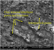
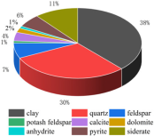
Processes 11 03131 i001Processes 11 03131 i002
PF BMedian porosity, median TOC, and high brittleness index; interparticle pores and intraparticle pores.Processes 11 03131 i003Processes 11 03131 i004
PF CLow porosity, median TOC, and low brittleness index; clay mineral interlayer pores and fractures, and sparsely developed interparticle and intraparticle pores.
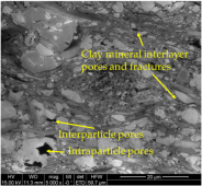
Processes 11 03131 i005Processes 11 03131 i006
PF DUltra-low porosity, low TOC, and high brittleness index; clay mineral interlayer pores and fractures.Processes 11 03131 i007Processes 11 03131 i008
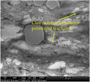
Disclaimer/Publisher’s Note: The statements, opinions and data contained in all publications are solely those of the individual author(s) and contributor(s) and not of MDPI and/or the editor(s). MDPI and/or the editor(s) disclaim responsibility for any injury to people or property resulting from any ideas, methods, instructions or products referred to in the content.

