Dynamic Monitoring of Low-Yielding Gas Wells by Combining Ultrasonic Sensor and HGWO-SVR Algorithm

Abstract

As gas wells enter the middle and late stages of production, they will become low-yielding gas wells due to fluid loading and insufficient formation pressure. For many years, there has been a lack of effective dynamic monitoring methods for low-yielding gas wells, and it is difficult to determine the production of each phase in each production layer, which makes further development face great uncertainty and a lack of basis for measurement adjustment. In order to solve this problem, this paper proposes an intelligent dynamic monitoring method suitable for low-yielding gas wells, which uses an ultrasonic Doppler logging instrument and machine learning algorithm as the core to obtain the output contribution of each production layer of the gas well. The intelligent dynamic monitoring method is based on the HGWO-SVR algorithm to predict the flow of each phase. The experimental data are selected for empirical analysis, and the effectiveness and accuracy of the method are verified. The research shows that this method has good application prospects and can provide strong technical support for gas reservoir production stability and development adjustment.

1. Introduction

With the deepening of the exploration and development of oil and gas fields, the dynamic monitoring technology of oil and gas reservoirs comes into being. Through dynamic monitoring technology, workers can effectively grasp the dynamic changes of oil and gas formations, which can help workers to do more research on the dynamic adjustment of oil and gas wells. At the same time, it can provide a perfect scientific basis for the relevant problems of oil and gas field exploitation, so as to effectively ensure the orderly development of oil and gas well exploitation.

Gas–liquid two-phase flow widely exists in petrochemical, energy power, nuclear reactor, aerospace, and other industrial fields; the study of gas–liquid two-phase flow is of great significance to the safe production in such related fields [1,2,3,4]. Production profile logging is an important monitoring technology in the development of oil and gas reservoirs; using the data can obtain the properties and production of the fluid produced by each reservoir [5]. With the continuous development of gas reservoirs, the gas production is gradually weakened, accompanied by the production of formation water. At this time, the low-velocity gas–liquid two-phase flow will occur in the well, and a large amount of liquid will appear at the bottom of the well, which seriously affects the normal production of gas wells. Due to the complex relative motion and interaction of the phase interface in the gas–liquid two-phase flow in the wellbore, it is extremely difficult to measure the split-phase flow rate and gas holdup, and the conventional gas–liquid two-phase production profile logging methods and interpretation models are not applicable. It is urgent to establish a new low-velocity gas–liquid two-phase flow production profile logging interpretation model.

In the gas–liquid two-phase flow, the interface of the gas–liquid two-phase structure is complex and changeable. To describe the change law of gas–liquid two-phase flow in more detail, scholars define the distribution state of fluid in the pipeline as the flow pattern. The formation of the flow pattern depends on the fluid density, viscosity, pipe diameter, and the flow rate of each phase, among which the flow rate of each phase plays the most important role. After numerous physical experiments, our predecessors divided the gas–liquid two-phase flow pattern of the vertical rising pipeline into bubbly flow, slug flow, churn flow, and annular flow [6,7,8].

The development of computational fluid dynamics has greatly promoted the research of the flow characteristics of gas–liquid two-phase flow in pipes. The VOF model has been widely used to solve multiphase flow problems since its development [9]. In 2008, Schepper et al. established a 3D horizontal pipeline model and used the VOF model and PLIC method to calculate the flow condition of the air and water in the horizontal pipeline, and the calculation results could be reproduced in Baker’s horizontal well flow pattern distribution map [10]. In 2016, Lopez et al. carried out physical experiments and CFD calculations on the gas–liquid two-phase flow in horizontal tubes. By comparing the experimental and numerical simulation results, the results show that the VOF multiphase flow model and SST k-ω can determine the gas–liquid two-phase flow pattern [11]. In 2020, Garcia et al. discussed the application of the VOF model in ANSYS-Fluent software (ANSYS FLUENT Release 15.0) to slug flow in two-dimensional horizontal pipelines, and proposed a reduced-order model for predicting the nonlinear flow dynamics of laminar liquid–liquid flow [12]. In the same year, to deepen the understanding of the transient characteristics of gas–liquid two-phase slug flow in horizontal pipelines, Deendarlianto et al. conducted CFD numerical simulation and experimental research on relevant phenomena [13]. In 2023, Zhao et al. simulated the gas–liquid two-phase flow pattern of horizontal and near-horizontal wells by using the VOF model, which was consistent with the experimental observation [14].

The most commonly used instruments for production profile logging in gas fields are spinner flowmeters (including collectors flow and arrays) and optical fiber gas holdup meters. However, the nonlinear response and low resolution of the instruments make the measurement accuracy not ideal under low flow rates. With the development of science and technology, more and more technologies are being used to measure gas–liquid two-phase flow parameters, including the capacitive method or conductometric method [15], optical fiber method [16], microwave method [17], gamma ray attenuation method [18], ultrasonic method [19], etc. These measurement methods have their characteristics, and ultrasonic wave has unique advantages in medical and pipeline fluid parameter monitoring because it generally does not damage the measured flow field in the process of propagation and can achieve non-invasive and non-disturbing parameter detection [20,21]. Currently, widely used ultrasonic methods include the reflection method, transmission method, Doppler method, and imaging method [22]. In 2004, Vatanakful et al. used a transmissive ultrasonic sensor to measure the dispersed phase holdup in a gas–liquid-solid three-phase flow [23]. Zheng et al. studied the effect of gas phase and solid phase on the response of an ultrasonic sensor in a gas–liquid-solid three-phase flow by measuring the velocity and attenuation of ultrasonic waves through the medium [24]. In 2016, Gong et al. suggested an ultrasonic pulse transmission method based on the ultrasonic sound pressure attenuation theory for monitoring gas holdup in gas–liquid two-phase bubble flow [22]. In 2020, Jin et al. used ultrasonic sensors and optical fiber sensors to investigate the measurement characteristics of gas holdup by ultrasonic sensors for typical flow patterns in oil–gas–water three-phase flows vertically rising with an inner diameter of 20 mm [25].

The Doppler effect is the basis for the ultrasonic Doppler method of flow measurement. The received signal frequency that is reflected or scattered on the sensor varies when the fluid being detected contains minute-moving bubbles or suspended particles. The fluid flow rate is then quantitatively measured by the frequency change value. In 2022, to explore the problem of the production profile logging of low-yield oil wells, Song et al. conducted an oil–water two-phase experimental investigation of ultrasonic Doppler logging tools based on the measurement theory of ultrasonic Doppler logging tools. Through the DCA and PCA methods, the water cut calculation chart and the ultrasonic oil flow rate prediction model are established and used in field interpretation, with a good application effect [26]. Wang et al. proposed a novel approach to production profile logging that used a converging annular logging tool and an ultrasonic Doppler logging tool to precisely determine the flow rate of each phase of an oil–water two-phase flow at a low flow rate, and verified its measurement characteristics through experiments. Last but not least, the PLS-SVR model was established to predict the flow rate of oil and water, and compared with the measured value, the results show high accuracy [5].

With the rise of artificial intelligence and society as a whole, more and more industries have bid farewell to traditional production methods, but have combined traditional equipment with modern scientific and technological means to enter an era of intelligence. In the production profile logging of low-yield gas wells, the phase distribution and velocity distribution of gas–liquid two-phase fluid in the wellbore become complicated due to the influence of gas well fluid accumulation, which makes the existing conventional production profile logging interpretation methods such as the drift model and slippage model not applicable. To accurately determine the gas–liquid two-phase flow parameters, the relevant knowledge of machine learning is applied to the production profile logging interpretation model. Support vector regression (SVR) is a statistical learning-based machine learning approach primarily utilized for regression issues. It has been extensively utilized in financial forecasting, data mining, biomedicine, and other fields due to its superior performance when dealing with problems involving small samples, nonlinearity, high dimensionality, and others [27,28,29]. The prediction effect of the SVR algorithm is heavily influenced by the model parameters (penalty coefficient and kernel function parameters) that are chosen, despite its theoretical and practical advantages. Therefore, the question of how to select the appropriate parameters has always been a contentious and challenging aspect of SVR algorithm research. Cross-validation, gradient descent, grid search, and other methods are the traditional SVR parameter optimization methods [30,31,32], all of which have the disadvantages of huge computation amounts and large errors.

The swarm intelligence algorithm originates from imitation research on the behavioral laws of biological populations, mainly imitating the foraging process of individual biological populations. Given the foraging process of biological populations, it is abstracted into a certain swarm intelligence algorithm [33]. Since genetic algorithm (GA) and ant colony optimization (ACO) were proposed, domestic and foreign scholars have successively proposed particle swarm optimization (PSO), artificial fish swarm algorithm (AFSA), firefly algorithm (FA), bat algorithm (BA), fruit fly optimization algorithm (FOA), grey wolf optimizer (GWO), whale optimization algorithm (WOA), and other swarm intelligence algorithms [34]. The swarm intelligence algorithm has a strong robustness, extensibility, generality, and simplicity of implementation. Since it was first proposed, it has gained a lot of popularity. It has performed well in nonlinear parameter optimization problems and has been used to optimize SVR prediction model parameters [35,36,37,38].

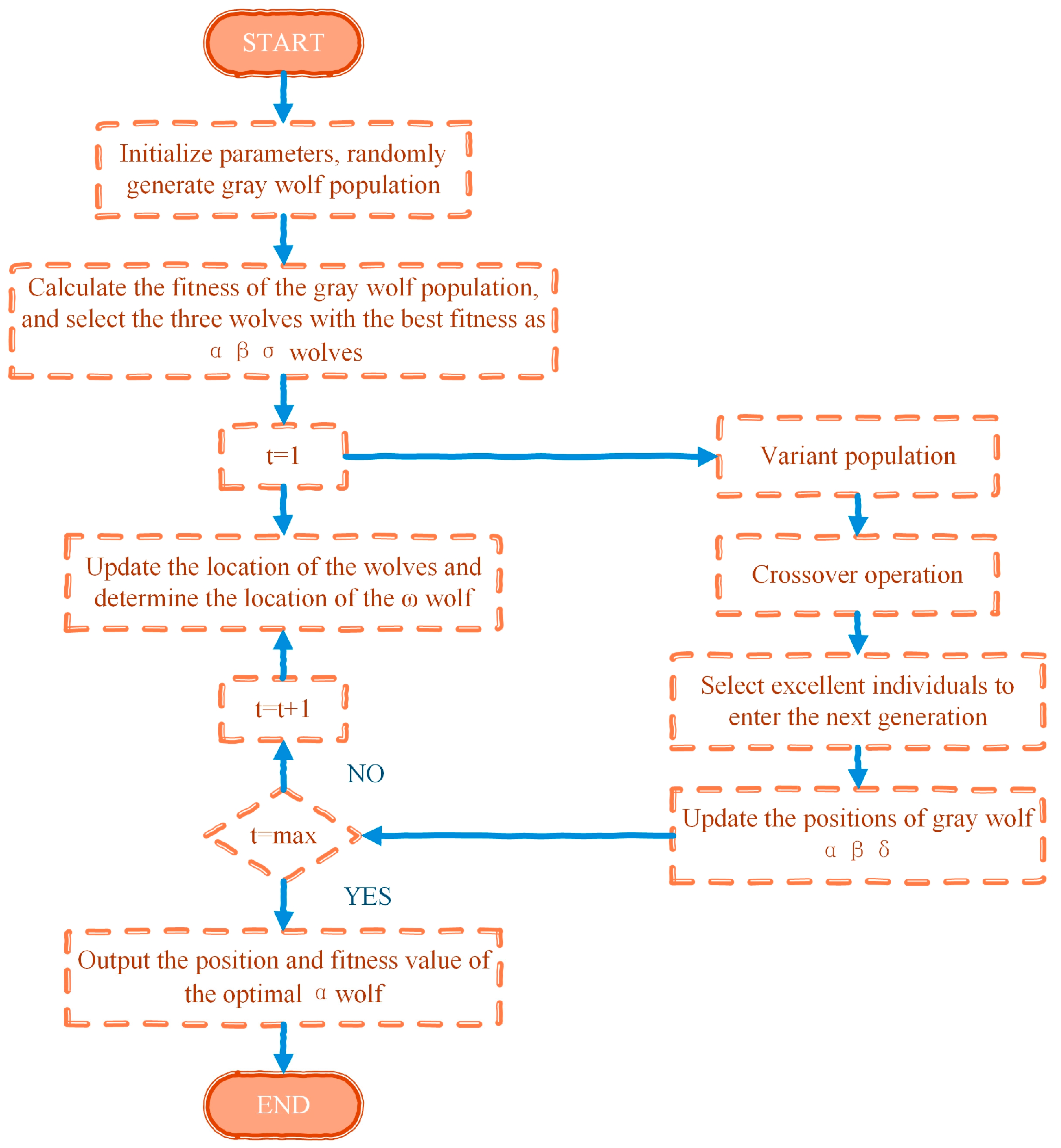
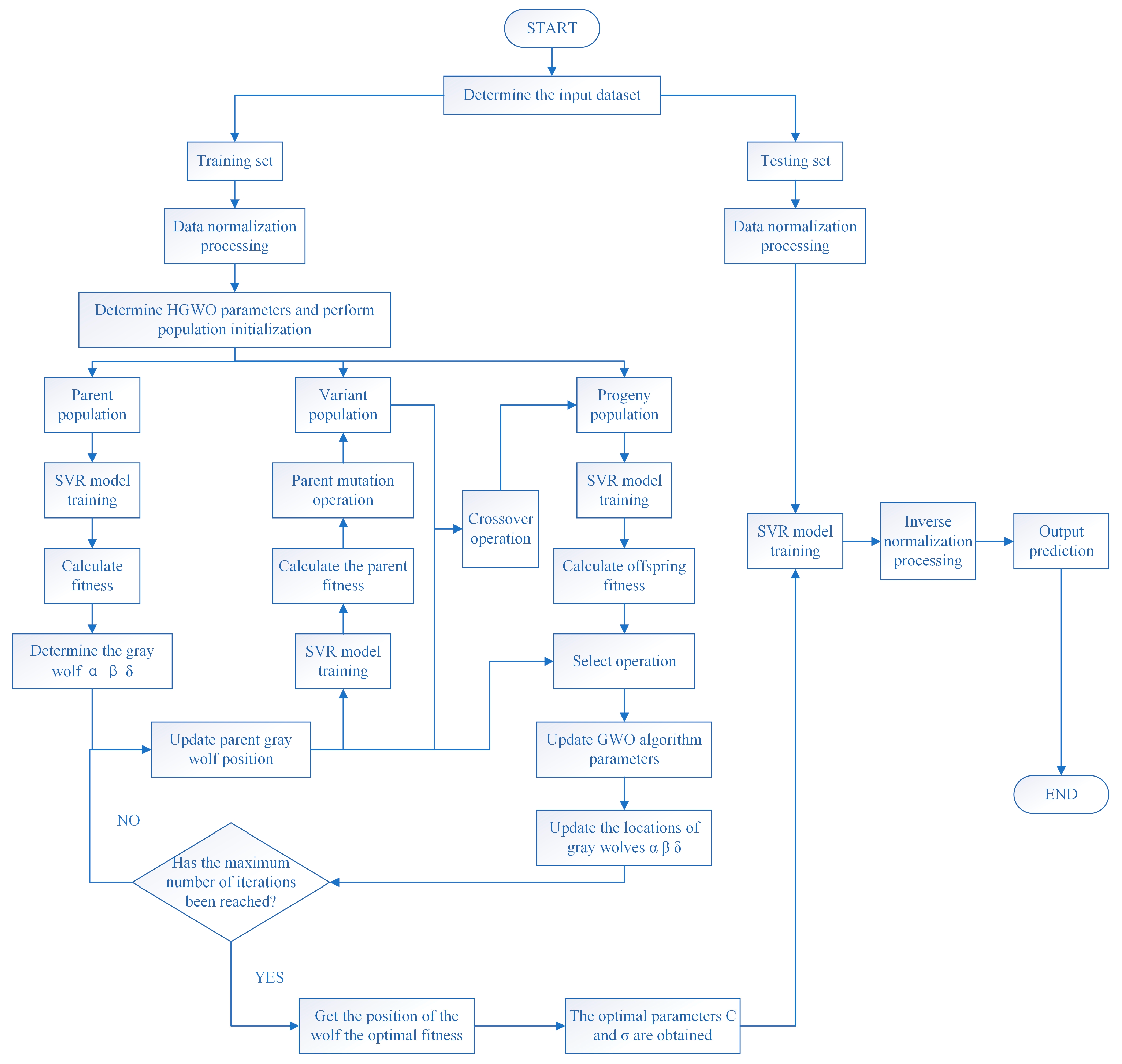
The flow pattern and velocity field distribution of gas–liquid two-phase flow at various phase flow rates are derived by numerically simulating the flow characteristics of low-velocity gas–liquid two-phase flow using CFD technology in this paper. The ultrasonic Doppler logging tool’s response to the different flow rates of gas–liquid two-phase flow is then examined through physical experiments. The correlation between the flow parameters and the characteristic parameters of the ultrasonic power spectrum was determined using distance correlation analysis. Finally, the parameters of the support vector regression prediction model were then optimized using the hybridizing gray wolf optimization with differential evolution, and the HGWO-SVR prediction model was established. Gas flow, gas holdup, and water flow are predicted, and the proposed combined optimization model’s effectiveness and accuracy are demonstrated.

2. Numerical Simulation

2.1. Creation and Meshing of Geometric Models

According to the pipe string structure of field production wells in oil and gas fields, this paper established a three-dimensional geometric model of vertical circular pipe with an inner diameter of 124 mm and a length of 20 m. The main body is a transparent plexiglass pipe, and the geometric model’s schematic is depicted in Figure 1a.

After the geometric model is established, meshing is a necessary process for solving, a prerequisite for subsequent iterative solutions, and a key step in the entire numerical simulation calculation. The quality of meshing will directly affect the accuracy of subsequent calculation results. When building the geometric model, the convenience of volume division should be considered as much as possible. When dividing the object into meshes, the boundary line (namely the pipe wall) to which the object is attached is restricted, and the mesh density of this edge is delimited, to better control the mesh classification using structured mesh in the mesh model. All mesh types of the section of the geometric model adopted in this paper are triangular free-surface mesh types, and the side sections are divided into 1000 elements. The minimum element size of the section (circular plane) is 0.005 m, which is the order of linear elements, and is divided by program control and global variables. There are 569,569 nodes and 1,058,000 cells in total, as shown in Figure 1b,c.

2.2. VOF Multiphase Flow Model

In numerical simulations, the flow is treated as transient and the problem is three-dimensional, so computational fluid dynamics (CFD) methods must be used to solve it. This polyphase coding can solve mass, momentum, and energy conservation equations and describe physically closed models through different methods and strategies. To solve the above problems, the flow characteristics of gas–liquid two-phase flow with low velocity in a vertical ascending pipe are simulated by using the VOF model of multiphase flow in computational fluid dynamics method.

In 1981, Hirt and Nichols first proposed the VOF model [9]. The VOF model is a surface tracking method built on a fixed Euler grid, which is an Euler method in which the fluid moves through a fixed computational grid or grid cells [13]. In this model, it is assumed that the two or more fluids involved in the simulated flow are incompatible with each other, but the fluids can be distributed within the computational domain at scales defined by the volume size of the computational grid [39]. In the VOF model, the computational domain is divided into small computational units, and the phase interface of each computational unit is tracked by introducing the phase volume fraction. Within each control volume, the sum of all phase volume fractions is 1. The attribute region assigned by all variables in the calculation domain is shared by all phase fluids, and this attribute is called volume average value. The volume fraction of any phase at any position is known. Therefore, whether the fluid properties in a given unit are single-phase or multiphase mixtures depends on the value of phase volume fraction. For example, in the gas–liquid two-phase flow, the volume fraction of liquid phase fluid is assumed to be denoted as ${\alpha }_l$ in the grid cell. When ${\alpha }_l$ is 0, it means that the grid cell does not contain liquid phase fluid, but is filled with gas phase fluid. When ${\alpha }_l$ is 1, it means that all the grid cells are filled with liquid fluid. When the value of ${\alpha }_l$ is between 0 and 1, it means that there is a gas–liquid two-phase fluid phase interface in the grid cell. The governing equations of the VOF multiphase flow model are as follows:

Phase volume fraction equation (continuity equation):

Tracking the interface between phases is accomplished by solving the continuity equation for the volume fraction of one or more phases. For the phase q, the equation is as follows:

$$\frac{\partial {\alpha }_q}{\partial t}+\overrightarrow{u}·\nabla {\alpha }_q=\frac{S_{{\alpha }_q}}{{\rho }_q}$$

(1)

In Equation (1), ${\alpha }_q$ represents the volume fraction of phase q; $t$ stands for time, s; $\overrightarrow{u}$ is the velocity vector, m/s; $S_{{\alpha }_q}$ is the mass source term. By default, the right source phase of Equation (1) is zero, but it is not zero when you specify a constant or user-defined mass source for each phase. ${\rho }_q$ represents the fluid density of phase q. The calculation of the volume fraction of the main phase is based on the constraints of Equation (2):

$${{\displaystyle \sum }}_{q=1}^n{\alpha }_q=1$$

(2)

Phase property equation:

The properties that appear in the transport equations are determined by the phasing present in each control volume. In general, for the n-phase system, the average density is calculated using Equation (3):

$$\rho ={{\displaystyle \sum }}_{q=1}^n{\alpha }_q{\rho }_q$$

(3)

Momentum equation:

By solving a single momentum equation over the entire region, the resulting velocity field is shared by the phases. The momentum equation depends on the volume ratio of all phases through the properties $\rho$ and $\mu$, and the equation is as follows:

$$\frac{\partial }{\partial t}\left(\rho \overrightarrow{u}\right)+\nabla ·\left(\rho \overrightarrow{u}\overrightarrow{u}\right)=-\nabla p+\left[\mu \left(\nabla \overrightarrow{u}+\nabla {\overrightarrow{u}}^T\right)\right]+\rho \overrightarrow{g}+\overrightarrow{F}$$

(4)

In Equation (4), $\mu$ is the hydrodynamic viscosity, Pa·s; $\overrightarrow{g}$ is the acceleration of gravity, m/s²; $\overrightarrow{F}$ is the surface tension, N/m³; $p$ is the pressure, Pa.

Energy conservation equation:

The energy equation is also shared among the phases and is expressed as follows:

$$\frac{\partial }{\partial t}\left(\rho E\right)+\nabla ·\left[\overrightarrow{u}\left(\rho E+p\right)\right]=\nabla ·\left(k_{eff}\nabla T\right)+S_h$$

(5)

In Equation (5), $E$ represents the total energy, including internal energy, kinetic energy, and potential energy, J/kg; $k_{eff}$ denotes the effective heat conductivity, W/(m·K); $T$ stands for temperature, K; $S_h$ represents the source term, including radiation and other user-defined volumetric heat sources. $E$ in Equation (5) is mass-averaged to obtain Equation (6).

$$E=\frac{{{\displaystyle \sum }}_{q=1}^n{\alpha }_q{\rho }_q{E}_q}{{{\displaystyle \sum }}_{q=1}^n{\alpha }_q{\rho }_q}$$

(6)

In Equation (6), $E_q$ represents the energy shared by phase $q$.

2.3. Boundary Conditions and Control Parameter Settings

For simulating gas–liquid two-phase flow, this paper makes use of water and air as fluid materials, both of which are incompressible fluids, and their heat transfer is negligible. Since the flow of air and water is an incompressible flow, the properties of the fluid such as density and viscosity are not affected by temperature and pressure, and the fluid density and viscosity are constant constants.

Table 1. Simulate the physical properties of fluid media.

Fluid Material	$\mathit{\rho }$ (kg/m3)	$\mathit{\mu }$ (Pa·s)	$\mathit{\sigma }$ (N/m)
air	1.23	1.7894 × 10−5	0
water	998.2	0.001003	0.072

depicts the fluid medium’s physical parameters used in the simulation. The inlet (below the pipe) boundary of the pipe selects the velocity inlet boundary, and the outlet (above the pipe) boundary selects the pressure outlet boundary; the surrounding wall is still considered a no-slip wall surface, selection pressure solver for transient simulation; the simulation of environmental pressure is set to the standard atmospheric pressure; considering the influence of gravity and surface tension factor, the acceleration of gravity g = 9.8 m/s² is set along the straight direction of the pipeline.

This paper mainly studies the fluid charging problem in the vertical circular tube. To better deal with the problem of the distribution of fluid velocity field at the same time in the complex interface, complex surface, and all points of space in the two-phase flow, the VOF model is selected according to the principle that the multiphase flow model is selected under the condition of simplified simulation. Among them, the $\epsilon$ model is selected for the turbulence model. The k-ε model has the characteristics of wide application range and reasonable solution accuracy, and the effect of solving the fully developed turbulence issue is better. The following are the equations for the k-ε model’s dissipation rate $\epsilon$ and turbulent kinetic energy $k$:

$$\frac{\partial }{\partial t}\left(\rho k\right)+\frac{\partial }{\partial X_i}\left(\rho k{u}_i\right)=\frac{\partial }{\partial X_j}\left[\left(\mu +\frac{{\mu }_t}{{\sigma }_k}\right)\frac{\partial k}{\partial X_j}\right]+G_k+G_b-\rho \epsilon -Y_M+S_k$$

(7)

$$\frac{\partial }{\partial t}\left(\rho \epsilon \right)+\frac{\partial }{\partial X_i}\left(\rho \epsilon u_i\right)=\frac{\partial }{\partial X_j}\left[\left(\mu +\frac{{\mu }_t}{{\sigma }_{\epsilon }}\right)\frac{\partial \epsilon }{\partial X_j}\right]+C_{1\epsilon }\frac{\epsilon }{k}\left(G_k+C_{3\epsilon }{G}_b\right)-C_{2\epsilon }\rho \frac{{\epsilon }^2}{k}+S_{\epsilon }$$

(8)

In Equations (7) and (8), $G_k$ represents the generation term of turbulent kinetic energy caused by the average velocity gradient. $G_b$ represents the generation term of turbulent kinetic energy caused by buoyancy; in compressible turbulence, the contribution of fluctuating expansion to the total dissipation rate is shown by $Y_M$. $S_k$ and $S_{\epsilon }$ represent the custom source terms of turbulent kinetic energy and dissipation rate. $C_{1\epsilon }$, $C_{2\epsilon }$, and $C_{3\epsilon }$ are constant, and generally take $C_{1\epsilon }$ = 1.44, $C_{2\epsilon }$ = 1.92, $C_{3\epsilon }$ = 0.09; ${\sigma }_k$ and ${\sigma }_{\epsilon }$ denote the turbulent Prandtl number of $k$ and $\epsilon$, respectively. Generally, ${\sigma }_k$ = 1.0, ${\sigma }_{\epsilon }$ = 1.3; ${\mu }_t$ represents turbulent viscosity, and the calculation formula is shown in Equation (9).

$${\mu }_t=\rho C_{\mu }\frac{k^2}{\epsilon }$$

(9)

In Equation (9), $C_{\mu }$ is a constant, and generally, $C_{\mu }$ = 0.09.

The liquid phase is referred to as the secondary phase when employing the VOF model, while the gas phase is referred to as the prime phase. When setting the boundary conditions at the velocity inlet, it is necessary to input the average velocity of the inlet fluid, the volume fraction of the second phase fluid, the hydraulic diameter and turbulence intensity, and other model-related parameters. The hydraulic diameter is equal to the inner diameter of the vertical circular pipe, and the turbulence intensity needs to be calculated according to the Reynolds value. The following formula can be used to determine the Reynolds number $Re$ and the turbulence intensity $I$:

$$Re=\frac{D\overline{v}\rho }{\mu }$$

(10)

$$I=0.16\times R{e}^{-0.125}$$

(11)

In Equations (10) and (11), $D$ is the pipe inner diameter, m; $\overline{v}$ is the average flow rate of the fluid, m/s; $\rho$ is the fluid density, kg/m³; $\mu$ is the fluid viscosity, mPa·s.

At the middle and late stage of production, most gas wells will produce less than 5000 m³/d of surface gas per well, and some will even produce around 1000 m³/d. A low-velocity gas–liquid two-phase flow simulation scheme is designed in accordance with the actual situation of low-yield gas wells. The daily surface gas volume range is defined as 1000–4000 m³/d, and the total underground flow is designed to be 10, 20, and 30 m³/d, according to the gas volume coefficient (Bg) of the corresponding block being 1/130. The water cut of gas–liquid two phases is 10%, 30%, 50%, 70%, and 90%, a total of 15 simulation points.

2.4. Simulation Results and Analysis

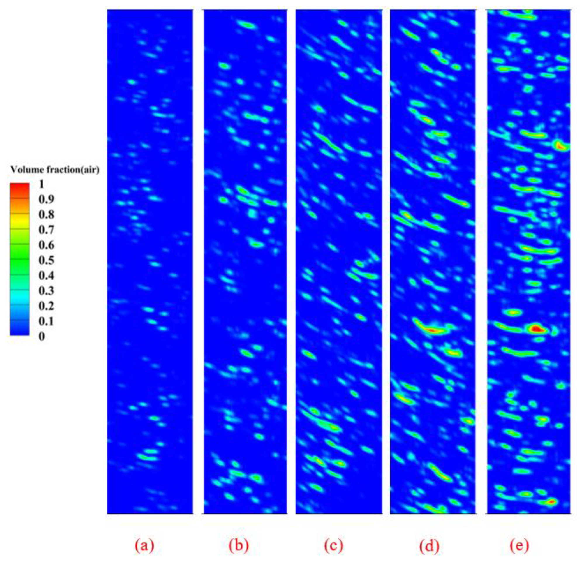
The study of the gas–liquid two-phase flow law is based on the flow pattern of gas–liquid two-phase flow. The flow pattern’s variation law is simulated using the simulation scheme for a variety of total flow rates and water cuts. Figure 2 shows the flow pattern distribution diagram under the condition of different water cuts with the total flow rate of gas–water two-phase 20 m³/d, which is presented in the form of a cloud map. Figure 2a–e, respectively, represent the distribution characteristics of gas–liquid two-phase flow patterns when the water cut is 90%, 70%, 50%, 30%, and 10%, in which blue represents liquid phase and red represents gas phase. It may be seen from Figure 2 that when the total flow rate of the gas–liquid two-phase is 20 m³/d, no matter how small the water cut is, the flow pattern is a typical bubbly flow. At this time, numerous bubbles will continue to be produced in the vertical circular tube, and the size and time interval of the bubbles are different. In the continuous liquid phase, the bubbles are not evenly distributed. Most of the bubbles exist in the pipeline in the shape of ellipses or narrow lengths, and the bubble diameter is much smaller than the inner diameter of the pipeline. With the continuous reduction in the water cut, that is, the continuous increase in the gas flow rate, the number and size of the bubbles in the pipeline continue to increase. Figure 3 shows the phase distribution diagrams under different total flow rates with a 10% water cut in the gas–water two-phase. The distribution characteristics of the gas–liquid two-phase flow patterns with total flow rates of 10 m³/d, 20 m³/d, and 30 m³/d, respectively, are depicted in Figure 3a–c. It is evident from Figure 3 that, in the event of the same water cut, an increase in the total flow rate will result in an increase in the relative number and size of the bubbles in the pipeline. In addition, it is possible to explain that the only flow pattern that exists for the gas–liquid two-phase low flow rate in the vertically rising pipeline is typical bubbly flow.

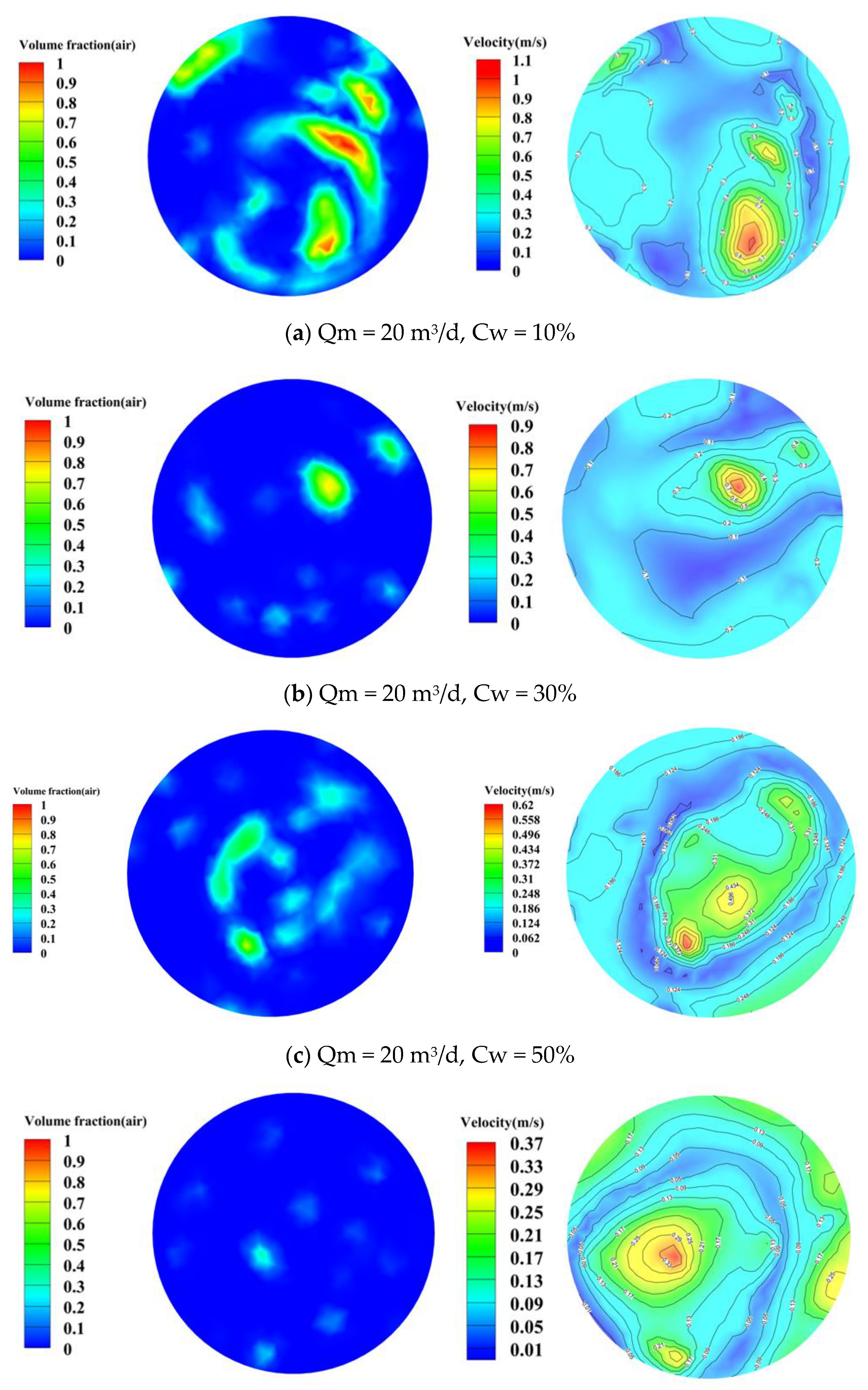
The gas–liquid two-phase flow velocity was used to further quantitatively characterize the characteristics of the gas–liquid two-phase flow, and the velocity distribution law was analyzed under various total flow rates and water cuts under bubble flow. This provided a foundation for determining the parameters of the gas–liquid two-phase interpretation model in low-yield gas wells. Figure 4 shows the distribution diagram of the phase state and velocity field under various water cuts with a total flow rate of 20 m³/d for the gas–water two-phase. The position intercepted is the XY plane at 12 m of the vertical pipeline. The left side is the phase state distribution diagram and the right side is the contour map of the velocity field. Combining the left and right figures, it can be seen that the velocity contour map at the position where the gas phase is located presents a high value, that is, the rising speed of bubbles in the vertical rising pipe is faster than that of water, and the overall velocity value of the gas–liquid two-phase exhibits a downward trend as the water cut increases. The maximum rising speed of bubbles with a 10% water cut is about 1.1 m/s, and then gradually decreases to about 0.24 m/s with a 90% water cut. 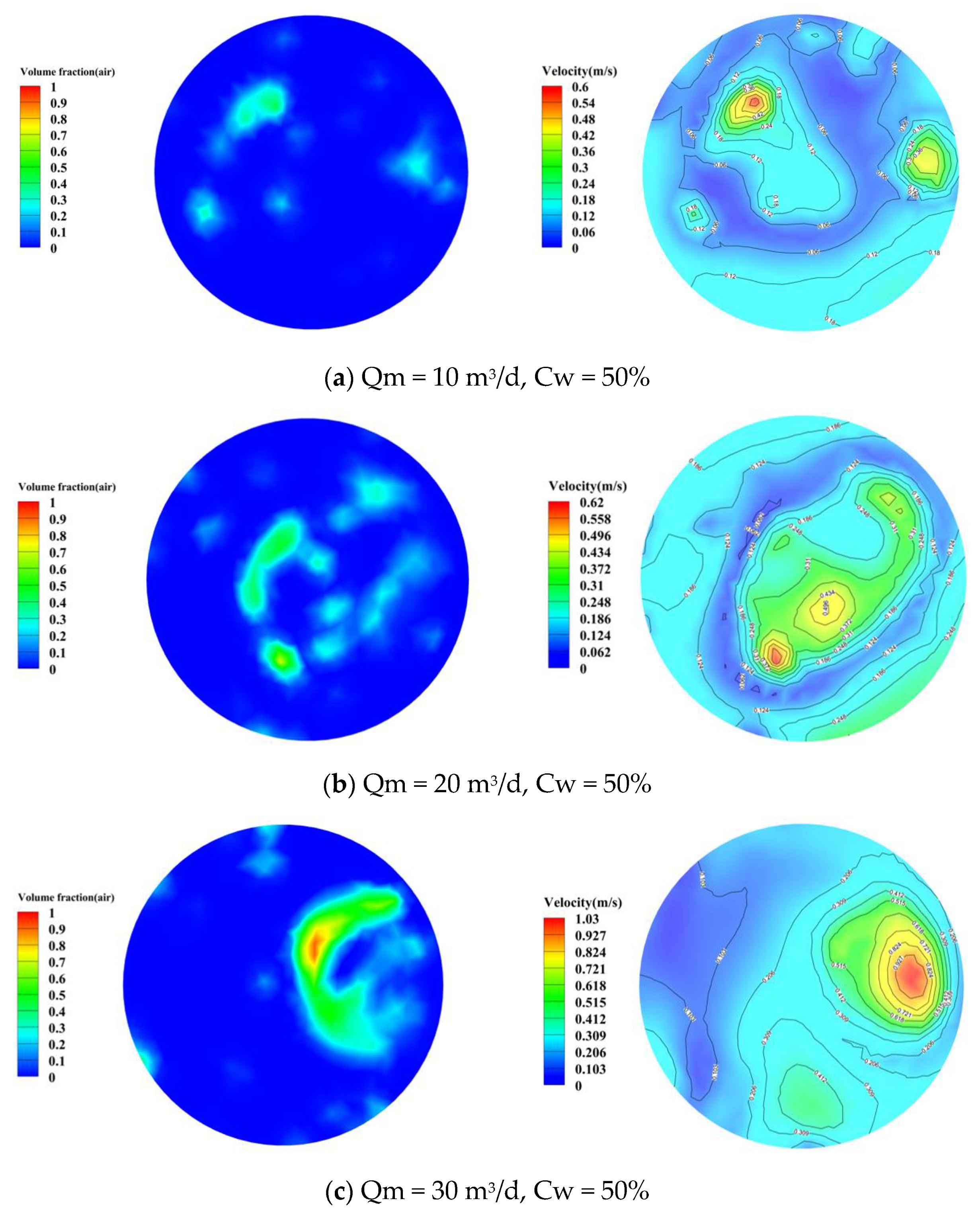Figure 5 shows the phase state distribution and velocity field distribution of the various total flow rates of the gas–water two-phase when the water cut is 50%. The overall velocity values of the gas–liquid two-phase show an upward trend with the increase in the total flow rate when the water cut is the same.

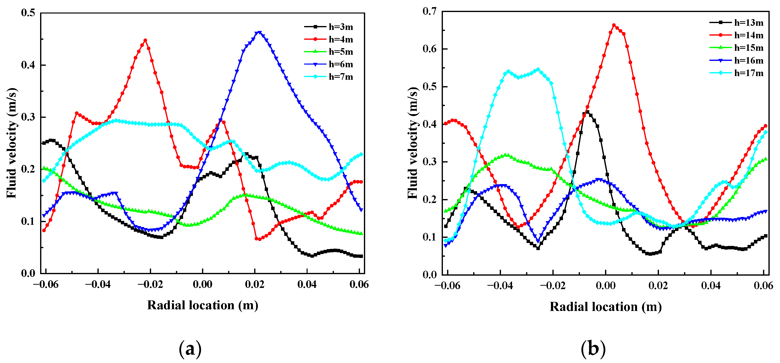
Figure 3b shows the flow pattern diagram of the gas–water two-phase flow rate of 20 m³/d and water cut of 10%. The position of the flow pattern diagram is the YZ plane at the center of the pipeline. The 20 m long pipeline was divided into upper and lower parts, and the bubbly flow in the middle of the upper and lower parts (3~7 m, 13~17 m) was divided at an equal interval of 1 m, respectively. The flow velocity of gas–liquid two-phase at this depth position was obtained, and the relationship between the flow velocity and the radial position of the pipeline was established, as shown in Figure 6. The different color curves in Figure 6 represent radial velocity profiles at different pipe heights. On the whole, each curve obviously presents an irregular peak-shaped distribution, and the peak positions of each curve are different. The peak positions of the fluid velocity curves represent the positions of the bubbles in the pipes.

As can be seen from Figure 6, the gas–liquid two-phase flow velocity range of the 3~7 m pipeline is 0.04~0.47 m/s, and the gas–liquid two-phase flow velocity range of the 13~17 m pipeline is 0.07~0.67 m/s. The steeper peak velocity of each curve represents the rising velocity of the bubbles, and the flatter part of the curve represents the flow velocity of the surrounding liquid phase. The overall velocity of the upper part is slightly higher than that of the lower part, and the overall curve is significantly more stable than that of the lower part. Overall, the interval of the fluid flow rate is increased when the increase in the pipe height decreases after a periodic first increase, which is mainly due to the pipe gas superficial velocity being low; the tube gas and liquid phase being in shearing action to promote each other by gas existing in the form of tiny air bubbles; and small bubbles rising constantly in the process of polymerization and bursting. The convergence of small bubbles into large bubbles will lead to an increase in the fluid velocity, and the collapse of large bubbles into small bubbles will lead to a decrease in the fluid velocity.

The gas holdup is of great significance to gas production profile logging, and its main purpose is to determine the fluid properties and assist in the calculation of the fluid flow rates in each phase. Gas holdup, also known as void fraction, refers to the proportion of the gas phase area to the total flow cross-section area in a two-phase flow [40]. When the gas–liquid two-phase flow is relatively stable in the numerical simulation, the gas holdup is calculated by replacing the area ratio with the ratio of the volume of the gas phase to the total volume. Figure 7 is the relationship between the gas holdup and the total flow rate and water cut of the gas–water two-phase obtained by the numerical simulation. When the total flow rate remains the same, it is evident that the gas holdup decreases as the water cut rises. When the water cut is the same, the gas holdup increases with the increase in the total flow rate, and the increase in the gas holdup decreases with the increase in the equal interval flow rate. In the low-velocity gas–liquid two-phase flow, the gas holdup value is very small, and the maximum gas holdup value in the figure is only 7.98%, which means that there will be a lot of liquid accumulation in the underground of the low-yield gas wells, which increases the difficulty of interpretation of the gas production profile logging data in low-yield gas wells.

3. Experiment

3.1. Experiment Setup

The dynamic simulation experiment of low flow rate gas–water two-phase flow was carried out on the multiphase flow simulation platform of a horizontal well with large deviation at Yangtze University. The experimental platform simulated the wellbore height of 12 m, the wellbore inner diameter of 124 mm and 159 mm. The material is a transparent plexiglass pipe, two kinds of transparent plexiglass pipe installed on a fixed frame connected to a U-shaped pipe, and the top and bottom of each pipe are installed with a fast-closing solenoid valve to ensure that the fluid can be closed instantly. A ruler with a minimum scale of 1 mm is fixed in the middle of the two pipes, which can help to measure the holdup by the quick-closing valve method. The schematic diagram of the experimental device is shown in Figure 8. The wellbore can be positioned in any direction, from horizontal to vertical. The inclination angle of the wellbore can be adjusted by a hydraulic drive, and the switch is set on the ground for manual control. The simulated flow range of the laboratory liquid phase is 0.2~600 m³/d, and the simulated flow range of the gas phase is 0.1~1000 m³/d. The gas phase and liquid phase are transported to the pressure regulator tank by an industrial grade peristaltic pump and then into the metering pipeline, which guarantees that the pump pulse has no effect on the fluid flow in the transport pipeline, and the high-precision mass flowmeter monitors the fluid in the transport pipeline online in real time. Then, the gas phase and liquid phase fluid enter the mixing tank, after mixing into the simulation wellbore. Through the online monitoring of the flow of the fluid flow parameters, and data into the computer, the console interface is used to adjust the gas phase liquid valve opening, and according to the experiment plan, the parameters are set by adjusting the input of the gas phase and liquid phase flow [41].

The wellbore angle was 90 degrees (a vertical well, in relation to the horizontal direction of the ground), the experimental fluid medium was air and tap water, and the experiment was carried out in a wellbore with an inner diameter of 124 mm. The specific experimental fluid parameters and experimental scheme are shown in

Table 2. Experimental fluid parameters and tests ranges.

Experimental Parameters	Units	Range
Air density (${\rho }_g$)	kg/m3	1.23
Water density (${\rho }_w$)	kg/m3	998.2
Air viscosity (${\mu }_g$)	Pa·s	1.7894 × 10−5
Water viscosity (${\mu }_w$)	Pa·s	0.001003
Operate pressure	MPa	0.1~0.15
Operate temperature	°C	25~30
Interfacial tension (${\sigma }_{g-w}$)	N/m	0.072
Test section diameter	mm	124
Gas flow rates ($Qg$)	m3/day	0~35
Water flow rates ($Qw$)	m3/day	0~35
Mixtures flow rates ($Qm$)	m3/day	5, 8, 10, 12, 15, 18, 20, 23, 25, 28, 30, 35
Water cut ($Cw$)	%	0~100

, with the input gas and water with different flow rates according to the experimental scheme. In order to guarantee that the fluid fully developed, we waited half an hour before starting the instrument for measurement after the ratio of gas–water flow at each experimental point was stable. The probe of the instrument was located 6.0 m from the fluid inlet of the simulated wellbore, and the image data of the flow pattern were recorded during the instrument’s measurement process. After the instrument test, the quick closing valve switch was opened through the console, and the calibration position of the phase interface was recorded after the gas–water phase interface was stable, to facilitate the subsequent experimental processing. We repeated the above experimental process to complete all the experimental points in turn.

3.2. Experiment Instrument

The instrument used in the low-velocity gas–water two-phase flow experiment is an ultrasonic Doppler multiphase flow logging instrument, as shown in Figure 9. During the experiment, the ultrasonic probe was positioned at the bottom of the instrument string, and the instrument string was connected with the centralizer, so that the instrument was centered for measurement (as shown in Figure 10). The diameter of the instrument was 23 mm, the maximum operating temperature was 150 °C, and the maximum working pressure was 60 MPa. The instrument adopts a non-collecting flow mode, does not affect the flow state of the downhole fluid, and can be measured in the sand wells, so that the test results are more accurate and are unaffected by the formation water salinity and fluid properties. The instrument’s measurement method is point measurement, and the collection speed is fast, with each test point test time being about 3 min. The basic measurement principle of the ultrasonic Doppler multiphase flow logging instrument can be found in [26].

3.3. Analysis of Experimental Data

Figure 11 shows the total flow of 20 m³/d of the gas–water two-phase recorded by the camera during the experiment, and the flow patterns of various water cuts. Figure 11a–e represent the flow patterns when the water cut is 90%, 70%, 50%, 30%, and 10%, respectively. It can be seen that the flow patterns are all bubbly flow, and with the decrease in the water cut, the relative number of bubbles and bubble diameter show an increasing trend, corresponding to the results obtained in the numerical simulation. Only one flow pattern, bubble flow, appears in the whole experimental process.

The frequency and amplitude are the initial data that the ultrasonic Doppler logging tool gathered. In order to eliminate the influence caused by accidental errors, 5–6 cycles of data are collected for each experimental point (as shown in Figure 12), and the frequency and amplitude data of this experimental point are obtained by calculating the average value. A power spectrum analysis was performed on the instrument’s logging data in order to investigate the ultrasonic Doppler logging instrument’s response to the bubble flow. The instrument’s measurement principle analysis shows that the strength of the ultrasonic emission signal, which is related to factors like the relative number of bubbles and the size of the bubble diameter at the experimental point, is reflected in the amplitude of the power spectrum curve. The relative velocity of the bubbles and other factors influence the frequency of the power spectrum curve. The power spectrum curves of the gas–water two-phase flow with various water cuts are depicted in Figure 13, using the total flow rates of 5 m³/d, 12 m³/d, 18 m³/d, and 25 m³/d as examples. The power spectrum that follows demonstrates that, under the condition of constant total flow, the peak amplitude decreases with an increasing water cut, with the decrease being more pronounced at a high water cut. This is primarily attributable to an increase in the water cut, which results in a decrease in the gas flow rate and the proportion of discrete bubbles in the continuous water phase. These factors weaken the ultrasonic wave reflection on the surface of the bubbles and reduce the reflected waves received by the ultrasonic probe, resulting in a decrease in the peak amplitude. For the same reason that was mentioned earlier, the peak amplitude increases with the increasing total gas–water two-phase flow under a constant water cut. The center frequency, on the other hand, did not significantly alter with the water cut or total flow.

The characteristic parameters of the ultrasonic power spectrum, such as gas amplitude, gas frequency, gas variance, and gas peak area, which reflected the information on the bubble distribution and flow rate, were obtained using the Gaussian function to fit the power spectrum curve in order to mine additional data. The distance correlation analysis (DCA) method was used to analyze the gas flow rate, water flow rate, gas holdup measured by the quick-closing valve method, and the characteristic parameters of the ultrasonic power spectrum in order to determine the relationship between the gas–water two-phase flow parameters and these parameters. Specific data processing details can be found in [5]. The results are shown in Figure 14. The correlation between variables can be observed in the figure. The redder the color, the better the positive correlation between variables; the darker the blue or even the purplish color, the better the negative correlation between variables; the lighter the color (light green or light blue), the worse the correlation between variables. It can be seen from the results that the gas flow rate and gas holdup are well-correlated with many characteristic parameters, while the water flow rate is not strongly correlated with the characteristic parameters of the ultrasonic power spectrum. This is mainly related to the measuring principle of the instrument, which is more sensitive to the movement of bubbles. If only one or two parameters are used to calculate the oil or water flow rate by the traditional linear or nonlinear fitting formula, the results obtained will be greatly different from the real value. Some artificial intelligence algorithms can make full use of the characteristic information of each parameter to improve the interpretation accuracy of the phase flow.

4. Interpretation Model

4.1. Support Vector Regression (SVR)

In 1995, Corinna Cortes and Vapnik et al. proposed the support vector machine (SVM) algorithm [42], a type of statistical learning-based machine learning algorithm that has garnered widespread interest and development in recent years. As an extension of the support vector machine, support vector regression (SVR) is mostly used to solve function fitting and regression estimation problems. When it comes to solving high-dimensional, nonlinear, and small-sample pattern recognition and prediction problems, SVR has a number of distinct advantages. In order for the sample data to be as close to the hyperplane as possible, the core of the SVR model is to use a kernel function to map the sample data from the input space to the high-dimensional feature space. Next, the model looks for a decision function that can accurately reflect the distribution of the sample data in the high-dimensional feature space [43].

Detailed SVR implementation steps can be found in [5]. SVR is a type of supervised machine learning technique with a solid theoretical foundation. However, the model’s generalizability and prediction accuracy are directly influenced by the various SVR parameters. The parameters of the $ϵ-SVR$ model include the insensitive loss coefficient $ϵ$, the penalty coefficient $C$, and the kernel function parameter $\sigma$. The insensitivity loss coefficient $ϵ$ is related to the number of support vectors; the penalty coefficient $C$ affects the complexity and stability of the model; the kernel function parameter $\sigma$ reflects the distribution of samples in the feature space, and the three parameters affect each other and jointly determine the complexity and generalization performance of the SVR model. Therefore, selecting the parameters of SVR with precision and efficiency is necessary to improve the model’s prediction accuracy and generalization performance.

4.2. Hybridizing Gray Wolf Optimization (HGWO)

4.2.1. Basics of Gray Wolf Optimizer (GWO)

The swarm intelligence algorithm is an iterative optimization search algorithm, which has the characteristics of flexibility, global optimization, self-organization, and strong parallel processing ability, so it has become the most representative parameter optimization method for support vector regression, and has been successfully applied in many fields.

The grey wolf optimizer (GWO) is a novel pack intelligence optimization algorithm proposed by Australian Griffith University academics [44], which was inspired by the study of the strict social hierarchy and hunting behavior of gray wolf populations. The GWO algorithm achieves optimization based on the mechanism of wolf group cooperation by simulating gray wolf hunting behavior. It is easy to use, has few parameters that need to be changed, and has a simple structure. Mechanisms that can dynamically adjust the convergence factor and information feedback are among these. This allows the system to strike a balance between local optimization and global search, resulting in a good problem-solving accuracy and convergence speed.

It is possible to formulate the mathematical model of the gray wolf population’s hunting behavior, as in [44]:

(1)

Social Hierarchy

The gray wolf social hierarchy must be constructed first, and the fitness of each member of the population must be calculated before the gray wolf optimization algorithm can be designed. The wolf pack’s three gray wolves with the highest fitness (optimal solution) are designated as $\alpha ,\beta ,\sigma$, and the remaining gray wolves (candidate solution) are labeled as $\omega$.

(2)

Encircling Prey

During the hunt, the behavior of the gray wolf surrounding the prey was defined as follows:

$$\overrightarrow{D}=\left|\overrightarrow{C}·\overrightarrow{X_p}\left(t\right)-\overrightarrow{X}\left(t\right)\right|$$

(12)

$$\overrightarrow{X}\left(t+1\right)=\overrightarrow{X_p}\left(t\right)-\overrightarrow{A}·\overrightarrow{D}$$

(13)

Equation (12) denotes the distance that separates the individual from the prey, and Equation (13) is the gray wolf’s formula for updating its position. Where $t$ is the current iteration number, $\overrightarrow{X_p}$ and $\overrightarrow{X}$ are the position vector of the prey and the position vector of the gray wolf, respectively, and $\overrightarrow{A}$ and $\overrightarrow{C}$ are the coefficient vectors. The calculation formulas of $\overrightarrow{A}$ and $\overrightarrow{C}$ are as follows:

$$\overrightarrow{A}=2\overrightarrow{a}·\overrightarrow{r_1}-\overrightarrow{a}$$

(14)

$$\overrightarrow{C}=2\overrightarrow{r_2}$$

(15)

where $\overrightarrow{r_1}$ and $\overrightarrow{r_2}$ are random vectors in [0, 1], and $\overrightarrow{a}$ is a motion vector that decreases linearly from 2 to 0 over an iterative process.

(3)

Hunting

It is assumed that “$\alpha ,\beta ,\sigma$” have a strong ability to identify potential prey locations in order to simulate the search behavior of gray wolves. As a result, the positions of other search agents (including $\omega$) are updated in accordance with their location information after the best three gray wolves ($\alpha ,\beta ,\sigma$) in the current population are retained in each iteration. This behavior’s mathematical model can be expressed as follows:

$$\{\begin{array}{c}\overrightarrow{D_{\alpha }}=\left|\overrightarrow{C_1}·\overrightarrow{X_{\alpha }}-\overrightarrow{X}\right|\\ \overrightarrow{D_{\beta }}=\left|\overrightarrow{C_2}·\overrightarrow{X_{\beta }}-\overrightarrow{X}\right|\\ \overrightarrow{D_{\delta }}=\left|\overrightarrow{C_3}·\overrightarrow{X_{\delta }}-\overrightarrow{X}\right|\end{array}$$

(16)

$$\{\begin{array}{c}\overrightarrow{X_1}=\left|\overrightarrow{X_{\alpha }}-\overrightarrow{A_1}·\overrightarrow{D_{\alpha }}\right|\\ \overrightarrow{X_2}=\left|\overrightarrow{X_{\beta }}-\overrightarrow{A_2}·\overrightarrow{D_{\beta }}\right|\\ \overrightarrow{X_3}=\left|\overrightarrow{X_{\delta }}-\overrightarrow{A_3}·\overrightarrow{D_{\delta }}\right|\end{array}$$

(17)

$$\overrightarrow{X}\left(t+1\right)=\frac{\overrightarrow{X_1}+\overrightarrow{X_2}+\overrightarrow{X_3}}{3}$$

(18)

In Equation (16), $\overrightarrow{D_{\alpha }}$, $\overrightarrow{D_{\beta }}$ and $\overrightarrow{D_{\delta }}$ distributions represent the distances between $\alpha ,\beta ,\sigma$ and other individuals. $\overrightarrow{X_{\alpha }}$, $\overrightarrow{X_{\beta }}$ and $\overrightarrow{X_{\delta }}$ distributions represent the current positions of $\alpha ,\beta ,\sigma$; $\overrightarrow{C_1}$, $\overrightarrow{C_2}$, $\overrightarrow{C_3}$ are random vectors; $\overrightarrow{X}$ is the current location of the gray wolf. Equation (17) defines the step size and direction of individual $\omega$ in the wolf pack toward $\alpha ,\beta ,\sigma$, respectively. Equation (18) defines the final position of $\omega$.

(4)

Attacking Prey

According to Equation (14), as the attack prey model is being constructed, $\overrightarrow{A}$ is a random value in the interval [−$a$, $a$] and is decremented along with $\overrightarrow{a}$. We can force the gray wolves to attack the prey when $\left|A\right|<1$ and, conversely, force them to diverge from the prey in order to hopefully find a better prey when $\left|A\right|>1$. This will help the gray wolf optimizer’s global search capability.

(5)

Search for Prey

To find prey, gray wolves mainly rely on $\alpha ,\beta ,\sigma$ information. They begin by dispersing their search for the location of their prey before concentrating on attacking it. For the dispersion model, through $\left|A\right|>1$, it keeps its search agent from prey. This way of searching the GWO is a global search. $\overrightarrow{C}$ is another search coefficient in the GWO algorithm, as shown in Equation (15), in which the $\overrightarrow{C}$ vector is a random vector with values between 0 and 2 in the interval. This coefficient gives the prey a random weight that can either go up ($\left|C\right|>1$) or down ($\left|C\right|<1$). During optimization, this assists GWO in exhibiting random search behavior to prevent the algorithm from falling into local optima. It is important to note that $\overrightarrow{C}$ is not a linear decline; rather, $\overrightarrow{C}$ is a random value during the iterative process. This coefficient helps the algorithm get out of the local area, particularly in the later stages of the iteration.

4.2.2. Basics of Differential Evolution (DE)

A heuristic parallel search technique based on group differences, the differential evolution (DE) algorithm, was developed in 1997 by Storn and Price [45]. The original intention was to solve the Chebyshev polynomial fitting problem. As a new and efficient heuristic parallel search technology, the differential evolution algorithm has the characteristics of fast convergence, few control parameters, simple setting, and robust optimization results. It has important academic significance for the theoretical and application research of evolutionary algorithms. The DE algorithm’s main process can be broken down into four steps: population initialization, mutation, crossover, and selection. The following is a detailed description of these steps [45]:

(1)

Population initialization

Define the population size as $NP$ in the D-dimensional search space, and randomly generate $NP$ initial population individuals in the whole search space. The formula is as follows:

$$x_{ij}\left(0\right)=x_{ij}^L+rand\left(0,1\right)·\left(x_{ij}^U-x_{ij}^L\right) \left(i=1,2,\dots ,NP;j=1,2,\dots ,D\right)$$

(19)

In Equation (19), $x_{ij}^U$ and $x_{ij}^L$ are the upper and lower bounds of the individual population in the j-dimensional search space, respectively; rand (0, 1) denotes a random number that follows a uniform distribution between [0, 1].

(2)

Mutation

The mutation process of differential evolution is the key to differential evolution, and the mutant individuals are generated by the following formula:

$$v_{ij}\left(g+1\right)=x_{r1}\left(g\right)+F·\left(x_{r2}\left(g\right)-x_{r3}\left(g\right)\right)$$

(20)

In Equation (20), $g$ represents evolutionary algebra; $x_{r1}$, $x_{r2}$, $x_{r3}$ are three different parameter vectors randomly selected in the population, and $r1\ne r2\ne r3\ne i$; $F$ is the scaling factor between [0, 1].

(3)

Crossover

The crossover operation can increase the diversity of the population, and is operated as follows:

$$u_{ij}\left(g+1\right)=\{\begin{array}{c}{v}_{ij}\left(g+1\right),if rand\left(0,1\right)\le CR or j=rand\left(1,n\right)\\ x_{ij}\left(g\right),if rand\left(0,1\right)>CR and j\ne rand\left(1,n\right)\end{array}$$

(21)

In Equation (21), $CR$ is a number between 0 and 1, called the crossover probability.

(4)

Selection

In order to decide whether the test vector $u_i\left(g+1\right)$ will become a member of the next generation, the differential evolution algorithm compares the test vector with the target vector $x_i\left(g\right)$ in the current population according to the greedy criterion. The operation is as follows:

$$x_i\left(g+1\right)=\{\begin{array}{c}{u}_i\left(g+1\right), f\left[u_i\left(g+1\right)\right]<f\left[x_i\left(g\right)\right]\\ x_i\left(g\right), f\left[u_i\left(g+1\right)\right]\ge f\left[x_i\left(g\right)\right]\end{array}$$

(22)

where $f$ is the fitness function, and here corresponds to the minimization problem. From the selection process of differential evolution, it can be seen that the result of the low fitness of the differential evolution algorithm replaces the original result, that is, the better result produced after mutation replaces the previous poor result, which plays the role of optimization selection and makes the whole population closer in the direction of optimization.

4.2.3. Hybridizing Gray Wolf Optimization with Differential Evolution (HGWO)

Using the differential evolution algorithm and gray wolf optimizer algorithm to solve optimization problems prone to premature aloneness, poor stability, easily falling into the local most superior defects, and through integrating the advantages and disadvantages of the two algorithms, Zhu et al. [46] proposed a hybrid optimizer that combined differential evolution with gray wolf optimization (HGWO), also known as the DE-GWO algorithm. Figure 15 depicts the algorithm flow chart. Firstly, in order to avoid the population iteration to a certain area, the phenomenon of the difference decreases. The crossing and selection operation of the difference optimization algorithm is used to maintain the diversity of the population. As the initial population of the wolves optimization algorithm, calculate the individual objective function values, and choose the best three individual $X_{\alpha }$, $X_{\beta }$ and $X_{\delta }$, according to the updated position of the other wolves. Then, the crossover and selection operations of the differential evolution are used to update the positions of the individual gray wolves, and the update is repeated iteratively until the optimal output of objective function value is selected. The hybrid algorithm not only improves the global search ability but also can effectively avoid the defects of premature stagnation and falling into local optimum.

4.3. The HGWO-SVR Model

In this paper, the improved gray wolf optimization algorithm based on differential evolution is used to optimize the penalty coefficient $C$ and the kernel function parameter $\sigma$ in the support vector regression model. The penalty coefficient $C$ and the kernel function parameter $\sigma$ are mapped to the position of the optimal wolf $\alpha$ in the gray wolf population, and the position of the optimal solution of the gray wolf population obtained in this way is used as the value of these two parameters in the support vector regression model. Figure 16 depicts the HGWO-SVR algorithm’s flowchart, and the specific steps of model building are as follows:

(1)

Divide the input data into a training set and test set, and normalize them.

(2)

Set the parameters of the HGWO algorithm: population size, maximum number of iterations, crossover probability, scale factor range, search dimension, and search range. Initialize the SVR parameters: set the value range of penalty coefficient $C$ and kernel function parameter $\sigma$.

(3)

Initialize the population, randomly generate the parent, mutant, and offspring gray wolf population, and set the number of iterations to one.

(4)

Train the SVR prediction model using the processed training set data.

(5)

Calculate the fitness of each individual gray wolf in the population, sort according to the size of the fitness function, and select the first three wolves as $\alpha ,\beta ,\sigma$ wolves, respectively, and record and save the positions of these three wolves.

(6)

According to Equations (16)–(18), update the positions of the other gray wolf individuals, except the $\alpha ,\beta ,\sigma$ wolves.

(7)

Use Equation (20) to perform the mutation operation in the differential evolution algorithm on the gray wolf individual to generate the intermediate individual, and perform the crossover processing according to Equation (21) to retain the high-quality part of the population, and perform the selection operation.

(8)

Recalculate the fitness of each individual in the population, update the fitness values of the $\alpha ,\beta ,\sigma$ wolves and their corresponding positions.

(9)

Determine whether the total number of iterations has been reached, if so, the algorithm will stop and output the position $X_{\alpha }$ of the global optimal solution $\alpha$ wolf, otherwise, go back to step 4.

(10)

The SVR prediction model is constructed by taking the position $X_{\alpha }$ of the $\alpha$ wolf as the value of the penalty coefficient $C$ and the kernel function parameter $\sigma$ in the SVR model.

4.4. Model Application

Based on the results of the ultrasonic Doppler experimental data and correlation analysis of the ultrasonic power spectrum characteristic parameters with the gas–water two-phase flow parameters at low flow rates, the amplitude peak, center frequency, gas amplitude, gas frequency, gas variance, gas peak area, amplitude ratio, and logarithm of the amplitude ratio of each group of experimental data are the input variables, and the gas flow rate and gas holdup of each group of experimental data are the output variables. There were a total of 77 sets of experimental data, 67 sets of data as the training set, 10 sets of data as the test set. To validate the effectiveness of the HGWO-SVR algorithm, both the support vector regression (SVR) and back propagation (BP) neural network algorithms are used for the prediction of the gas flow and gas holdup. When using the HGWO-SVR model for prediction, we set the population size to 30, the maximum number of iterations to 500, the upper bound of the scaling factor to 0.8, the lower bound to 0.2, the crossover probability to 0.1, and the convergence factor to dynamically decrease from 2 to 0. The SVR adopts the $ϵ-SVR$ model, and the kernel function adopts the most commonly used Gaussian kernel function in the radial basis function. The prediction results are shown in Figure 17, Figure 18 and Figure 19, and the prediction errors are shown in

Table 3. Statistical table of gas flow prediction error under different models.

	$\mathit{M}\mathit{S}\mathit{E}$	${\mathit{R}}^2$	$\mathit{M}\mathit{A}\mathit{E}/\left({\mathbf{m}}^3/\mathbf{d}\right)$	$\mathit{M}\mathit{A}\mathit{P}\mathit{E}/\left(\mathit{\%}\right)$
HGWO-SVR	0.00525	0.98861	0.547	6.146
SVR	0.02947	0.92665	1.472	14.011
BP	0.02169	0.93319	1.536	22.705

and

Table 4. Statistical table of gas holdup prediction error under different models.

	$\mathit{M}\mathit{S}\mathit{E}$	${\mathit{R}}^2$	$\mathit{M}\mathit{A}\mathit{E}/\left(\mathit{\%}\right)$	$\mathit{M}\mathit{A}\mathit{P}\mathit{E}/\left(\mathit{\%}\right)$
HGWO-SVR	0.00571	0.98491	0.197	6.278
SVR	0.02632	0.93247	0.470	12.526
BP	0.01343	0.94642	0.407	18.180

.

Figure 17 shows the fitness function curve of the HGWO-SVR model for predicting different output variables. The fitness function adopted by the model is the mean square error ($MSE$). When the output data is gas flow, the optimal fitness is 0.00525, the corresponding optimal parameter of penalty coefficient $C$ is 8.5421, and the optimal parameter of kernel function $\sigma$ is 0.6669. When the output data is gas holdup, the optimal fitness is 0.00571, the corresponding penalty coefficient $C$ optimal parameter is 13.1991, and the kernel function parameter $\sigma$ optimal parameter is 0.5888. Combining Figure 18 and Figure 19 and Table 3 and Table 4 reveals that the HGWO-SVR model’s prediction results are significantly superior to those of the SVR model and the BP neural network model and are closer to the actual data. Among them, the HGWO-SVR model has a mean absolute error of 0.547 m³/d in the prediction of gas flow in a low-velocity gas–water two-phase flow, and the accuracy is as high as 93.85%; the mean absolute error of the prediction of gas holdup is 0.197%, and the accuracy is as high as 93.72%. For the prediction results of the gas flow rate and gas holdup, the mean absolute percentage error of all the data of the HGWO-SVR model is less than 15%, and the mean absolute percentage error of most of the data is less than 5%. Figure 18 and Figure 19 also reflect the fact that the prediction accuracy of all models decreases when comparing high gas flow rate and high gas holdup. This has a strong relationship with the measurement principle of the ultrasonic Doppler logging instrument, which mainly probes the motion parameters of the discrete phase in the continuous phase. In the measurement of low-velocity gas–water two-phase flow, the instrument mainly measures the motion parameters of discrete bubbles. However, when these bubbles are more numerous and concentrated, its detection effect is not as good as that in the case of fewer bubbles, which will lead to the situation in Figure 18 and Figure 19. From Figure 14, it can be seen that the correlation between the water flow and characteristic parameters of each ultrasonic power spectrum is poor. The HGWO-SVR model is used to predict the water flow, and the results are shown in Figure 20. The optimal fitness of the model is 0.01676, the optimal parameter of the corresponding penalty coefficient $C$ is 32.0248, and the optimal parameter of the kernel function parameter $\sigma$ is 1.3581. The mean absolute error of the water flow prediction is 1.581 m³/d, and the mean absolute percentage error is 50.03%. When the water flow is large, the prediction error will be smaller.

Combining the correlation analysis with the model of the gas flow, the gas holdup and water flow prediction result shows that the ultrasonic Doppler tool in the low-velocity of gas–water two-phase flow monitoring can reflect well the status of the flow of the gas phase, and can accurately obtain the gas flow and the gas holdup. However, for the monitoring of the water flow conditions, the situation is a little worse, but in the case of a high water cut, the prediction accuracy of the water flow will be higher. This is due to the fact that the ultrasonic Doppler logging tool is mainly on the motion parameters of the continuous phase and discrete phase detection, and in the low-velocity gas–water two-phase flow, the flow pattern is bubbly flow, the water phase is the continuous phase and the gas phase in the bubbles form a water phase, so the instrument can accurately obtain the gas flow and the gas holdup. The measured water flow error is larger.

5. Conclusions

The dynamic monitoring of oil and gas wells is the key to the development of oil and gas fields. However, the current method based on conventional production profile interpretation cannot achieve the expected effect. The aim of this study was to test a practical approach for the dynamic monitoring of low-yielding gas wells using an ultrasonic Doppler logging instrument and a machine learning technique.

In the first part, the flow pattern and velocity field distribution of the gas–liquid two-phase flow with a low flow velocity are studied by CFD numerical simulation technology based on the production rate and well depth structure of actual produced low-yielding gas wells. It is found that the flow pattern is a typical bubbly flow when the gas–liquid two-phase flow has a low flow rate in the vertical riser pipeline, and the number and size of bubbles in the pipeline continue to increase with the continuous increase in the gas phase flow. The bubble rises faster than the water phase, and with the increase in the water cut, the overall velocity of the two phases decreases. In addition, in low-yielding gas wells, the water holdup is almost above 90%.

In the second part, the ultrasonic Doppler logging instrument is used to carry out a physical experiment examining the low velocity gas–liquid two-phase flow, and the characteristic parameters of the ultrasonic power spectrum under different gas–liquid two-phase flow conditions are obtained, and the gas holdup is obtained by the quick closing valve method. Through the distance correlation analysis between the flow parameters and the extracted ultrasonic power spectrum characteristic parameters in the process of gas–liquid two-phase flow at low flow rate, it is obtained that the gas flow and gas holdup have a good correlation with many ultrasonic power spectrum characteristic parameters. However, the water phase flow rate is not strongly correlated with the characteristic parameters of the ultrasonic power spectrum.

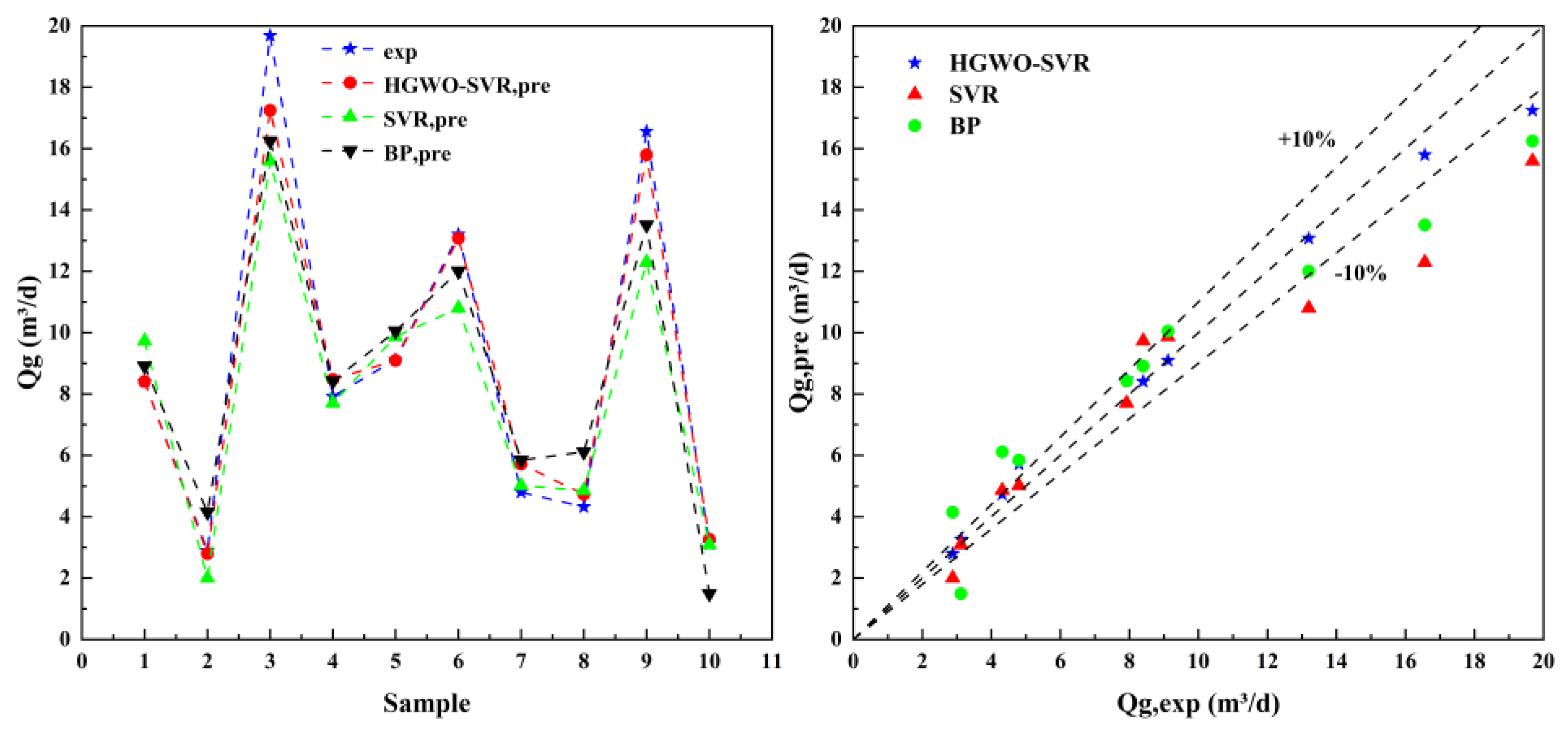
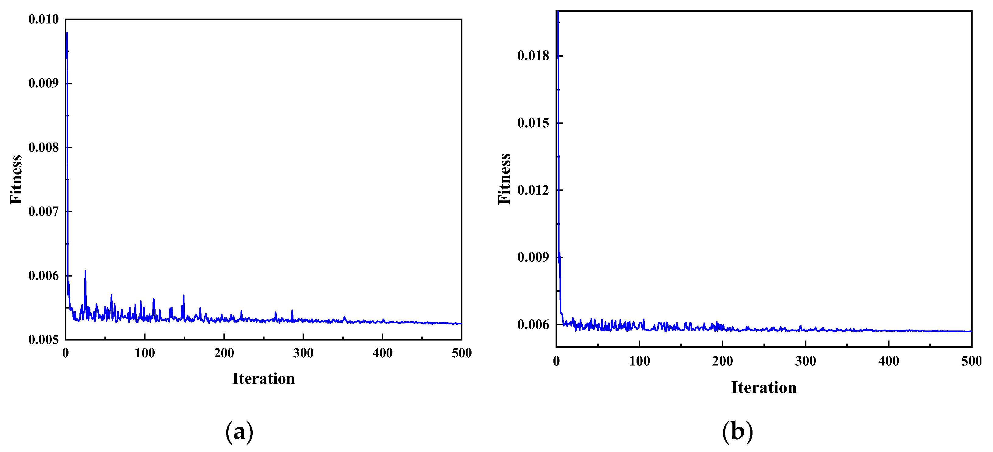
In the third part, the HGWO-SVR model is established to predict the flow parameters of the low flow rate gas–liquid two-phase, and the data set is based on the experimental data in the second part. Through the comparative analysis of the SVR and BP prediction methods, it is proved that the HGWO-SVR model has the best prediction effect, and the multiple prediction results are better. The HGWO-SVR model is adopted to predict the gas–liquid two-phase flow parameter, the gas flow rate and gas holdup have a good predictive effect, and the water flow prediction error is larger. The proposal in this situation of production profile logging using a gas stringer ultrasound Doppler tool and flow-concentrating spinner flowmeter is a combined measurement to improve the accuracy of water flow interpretation. It is suggested that the combination of the ultrasonic Doppler logging instrument and flow-concentrating spinner flowmeter should be used to improve the accuracy of the water phase flow interpretation when logging the production profile of low-yielding gas wells in fields.

References

1. Fang, L.D.; Liu, H.W.; Yousef, F.; Lan, K.; Guo, S.; Wang, F.; Zhu, Y. Study on measurement model of cross section holdup based on array ultrasonic sensor. Measurement 2022, 191, 110830. [Google Scholar] [CrossRef]
2. Thandlam, A.K.; Mandal, T.K.; Majumder, S.K. Flow pattern transition, frictional pressure drop, and holdup of gas non-Newtonian fluid flow in helical tube. Asia-Pac. J. Chem. Eng 2015, 10, 422–437. [Google Scholar] [CrossRef]
3. Shaban, H.; Tavoularis, S. Identification of flow regime in vertical upward air-water pipe flow using differential pressure signals and elastic maps. Int. J. Multiph. Flow 2014, 61, 62–72. [Google Scholar] [CrossRef]
4. Zheng, X.B.; Sun, X.D.; Bai, B.F. Flow rate measurement of low GVF gas-liquid two-phase flow with a V-Cone meter. Exp. Therm. Fluid Sci 2018, 91, 175–183. [Google Scholar] [CrossRef]
5. Wang, M.X.; Song, H.W.; Li, M.; Wu, C.Q. Prediction of split-phase flow of low-velocity oil-water two-phase flow based on PLS-SVR algorithm. J. Pet. Sci. Eng. 2022, 212, 110257. [Google Scholar] [CrossRef]
6. Hewitt, G.F.; Roberts, D.N. Studies of Two-Phase Patterns by Simultaneous X-ray and Flash Photography; Report AERE-M 2159; Atomic Energy Research Establishment: Harwell, UK, 1969. [Google Scholar]
7. Taitel, Y.; Barnea, D.; Dukler, A.E. Modelling flow pattern transitions for steady upward gas-liquid flow in vertical tubes. AIChE J. 1980, 26, 345–354. [Google Scholar] [CrossRef]
8. Mishima, K.; Ishii, M. Flow regime transitions criteria for upward two phase flow in vertical tubes. Int. J. Heat Mass Transf. 1984, 27, 723–737. [Google Scholar]
9. Hirt, C.W.; Nichols, B.D. Volume of fluid (VOF) method for the dynamics of free boundaries. J. Comput. Physics. 1981, 39, 201–225. [Google Scholar] [CrossRef]
10. De Schepper, S.C.K.; Heynderickx, G.J.; Marin, G.B. CFD modeling of all gas-liquid and vapor-liquid flow regimes predicted by the Baker chart. Chem. Eng. J. 2008, 138, 349–357. [Google Scholar] [CrossRef]
11. López, J.; Pineda, H.; Bello, D.; Ratkovich, N. Study of liquid-gas two-phase flow in horizontal pipes using High Speed Filming and Computational Fluid Dynamics. Exp. Therm. Fluid Sci. 2016, 76, 126–134. [Google Scholar] [CrossRef]
12. García, D.E.; Rodríguez, D.; Nieckele, A.O.; de Paula, I.B. Nonlinear instability of interfacial waves in stratified laminar channel flow. Int. J. Multiph. Flow 2020, 113, 103463. [Google Scholar] [CrossRef]
13. Andrianto, M.; Widyaparaga, A.; Dinaryanto, O. CFD Studies on the gas-liquid plug two-phase flow in a horizontal pipe. J. Pet. Sci. Eng. 2016, 147, 779–787. [Google Scholar]
14. Zhao, X.Y.; Song, H.W.; Wang, M.X.; Shi, X.L. Identification of Gas-Water Two-Phase Flow Patterns in Horizontal Wells of Shale Gas Reservoirs Based on Production Logging Data. Geofluids 2023, 2023, 6178829. [Google Scholar] [CrossRef]
15. Teixeira, C.E.; da Silva, L.E.B.; Veloso, G.F.C.; Lambert-Torres, G.; Campos, M.M.; Noronha, I.; Bonaldi, E.L.; de Oliveira, L.E.L. An ultrasound-based water-cut meter for heavy fuel oil. Measurement 2019, 148, 106907. [Google Scholar] [CrossRef]
16. Chen, K.; Zhu, D.; Hill, A.D. Acoustic Signature of Flow From a Fractured Wellbore. In Proceedings of the SPE Annual Technical Conference and Exhibition, Houston, TX, USA, 28–30 September 2015. [Google Scholar]
17. Nyfors, E.; Vainikainen, P. Industrial microwave sensors. In Proceedings of the 1991 IEEE MTT-S International Microwave Symposium Digest, Boston, MA, USA, 10–14 June 1991; pp. 1009–1012. [Google Scholar]
18. Roshani, G.H.; Feghhi, S.A.H.; Mahmoudi-Aznaveh, A.; Nazemi, E.; Adineh-Vand, A. Precise volume fraction prediction in oil–water–gas multiphase flows by means of gamma-ray attenuation and artificial neural networks using one detector. Measurement 2014, 51, 34–41. [Google Scholar] [CrossRef]
19. Ren, W.K.; Jin, N.D.; OuYang, L.; Zhai, L.S.; Ren, Y.Y. Gas Volume Fraction Measurement of Oil–Gas–Water Three-Phase Flows in Vertical Pipe by Combining Ultrasonic Sensor and Deep Attention Network. IEEE Trans. Instrum. Meas. 2020, 70, 2502409. [Google Scholar] [CrossRef]
20. Asher, R.C. Ultrasonic sensors in the chemical and process industries. J. Phys. E Sci. Instrum. 1983, 16, 959–963. [Google Scholar] [CrossRef]
21. Hauptmann, P.; Hoppe, N.; Puttmer, A. Application of ultrasonic sensors in the process industry. Meas. Sci. Technol. 2002, 13, 73–83. [Google Scholar] [CrossRef]
22. Gong, Z.; Zhao, A.; Zhai, L.S.; Ren, Y.Y. Ultrasonic method for measuring the gas holdup of gas-liquid bubbly flow in a small-diameter pipe. Korean J. Chem. Eng. 2016, 33, 1170–1180. [Google Scholar] [CrossRef]
23. Vatanakul, M.; Zheng, Y.; Couturier, M. Application of ultrasonic technique in multiphase flows. Ind. Eng. Chem. Res. 2004, 43, 5681–5691. [Google Scholar] [CrossRef]
24. Zheng, Y.; Zhang, Q.K. Simultaneous measurement of gas and solid holdups in multiphase systems using ultrasonic technique. Chem. Eng. Sci. 2004, 59, 3505–3514. [Google Scholar] [CrossRef]
25. Jin, N.D.; Ren, W.K.; Chen, X.; Zhai, L.S. Measurement of gas holdup in three phase flow using ultrasonic sensor. J. Appl. Acoust. 2020, 39, 36–44. [Google Scholar]
26. Song, H.W.; Li, M.; Wu, C.Q.; Wang, Q.C.; Wei, S.K.; Wang, M.X.; Ma, W.H. Data-Driven Methodology for the Prediction of Fluid Flow in Ultrasonic Production Logging Data Processing. Geofluids 2022, 2022, 1–15. [Google Scholar] [CrossRef]
27. Mishra, S.; Padhy, S. An efficient portfolio construction model using stock price predicted by support vector regression. North Am. J. Econ. Financ. 2019, 50, 101027. [Google Scholar] [CrossRef]
28. Quan, Q.; Zou, H.; Huang, X.F.; Lei, J.C. Research on water temperature prediction based on improved support vector regression. Neural Comput. Appl. 2020, 34, 8501–8510. [Google Scholar] [CrossRef]
29. Huang, J.C.; Tsai, Y.C.; Wu, P.Y.; Lien, C.Y.; Kuo, C.F.; Hung, J.F.; Chen, S.C.; Kuo, C.H. Predictive modeling of blood pressure during hemodialysis: A comparison of linear model, random forest, support vector regression, XGBoost, LASSO regression and ensemble method. Comput. Methods Programs Biomed. 2020, 195, 105536. [Google Scholar] [CrossRef]
30. Mao, W.T.; Xu, J.C.; Wang, C.; Dong, L.L. A fast and robust model selection algorithm for multi-input multi-output support vector machine. Neurocomputing 2014, 130, 10–19. [Google Scholar] [CrossRef]
31. Zou, Y.; Huang, Z.Y.; Hu, X.Y.; Xiao, J.W.; Li, J. Application of support vector regression algorithm optimized by gradient descent method for analysing efficiency of boiler. In Proceedings of the 2017 Chinese Automation Congress (CAC), Jinan, China, 20–22 October 2017; IEEE: Piscataway, NJ, USA, 2017; pp. 530–534. [Google Scholar]
32. Bao, Y.K.; Liu, Z.T. A fast grid search method in support vector regression forecasting time series. In Proceedings of the 7th International Conference on Intelligent Data Engineering and Automated Learning, Burgos, Spain, 20–23 September 2006; Springer: Berlin/Heidelberg, Germany, 2006; pp. 504–511. [Google Scholar]
33. Beni, G.; Wang, J. Swarm intelligence in cellular robotic systems. In Robots and Biological Systems: Towards a New Bionics; Springer: Berlin/Heidelberg, Germany, 1989; pp. 703–712. [Google Scholar]
34. Li, S.; Yuan, Z.G.; Wang, C.; Chen, T.E.; Guo, Z.C. Optimization of support vector machine parameters based on group intelligence algorithm. CAAI Trans. Intell. Syst. 2018, 13, 70–84. [Google Scholar]
35. Huang, J.; Bo, Y.C.; Wang, H.Y. Electromechanical equipment state forecasting based on genetic algorithm – support vector regression. Expert Syst. Appl. 2011, 38, 8399–8402. [Google Scholar] [CrossRef]
36. Zhang, D.M.; Liu, W.; Wang, A.; Deng, Q. Parameter Optimization for Support Vector Regression Based on Genetic Algorithm with Simplex Crossover Operator. J. Inf. Comput. Sci. 2011, 8, 911–920. [Google Scholar]
37. Salcedo-Sanz, S.; Ortiz-Garcıa, E.G.; Pérez-Bellido, Á.M.; Portilla-Figueras, A.; Prieto, L. Short term wind speed prediction based on evolutionary support vector regression algorithms. Expert Syst. Appl. 2011, 38, 4052–4057. [Google Scholar] [CrossRef]
38. Niu, M.F.; Hu, Y.Y.; Sun, S.L.; Liu, Y. A novel hybrid decomposition-ensemble model based on VMD and HGWO for container throughput forecasting. Appl. Math. Model. 2018, 57, 163–178. [Google Scholar] [CrossRef]
39. Storr, G.J.; Behnia, M. Comparison between experiment and numerical simulation using a free surface technique of free-falling liquid jets. Exp. Therm. Fluid Sci. 2000, 22, 79–91. [Google Scholar] [CrossRef]
40. Guo, H.M.; Song, H.W.; Liu, J.F. Production Logging Principle and Data Interpretation; Petroleum Industry Press: Beijing, China, 2021; pp. 21–62. [Google Scholar]
41. Song, H.W.; Guo, H.M.; Shi, X.L.; Shi, H.Y. Simulation logging experiment and interpretation model of array production logging measurements in a horizontal well. Appl. Geophys. 2021, 18, 171–185. [Google Scholar] [CrossRef]
42. Cortes, C.; Vapnik, V. Support-vector networks. Mach. Learn. 1995, 20, 273–297. [Google Scholar] [CrossRef]
43. Zhou, Z.H. Machine Learning; Tsinghua University Press: Beijing, China, 2016; pp. 121–140. [Google Scholar]
44. Mirjalili, S.; Mirjalili, S.M.; Lewis, A. Grey Wolf Optimizer. Adv. Eng. Softw. 2014, 69, 46–61. [Google Scholar] [CrossRef]
45. Storn, R.M.; Price, K. Differential Evolution—A Simple and Efficient Heuristic for Global Optimization over Continuous Spaces. J. Glob. Optim. 1997, 11, 341–359. [Google Scholar] [CrossRef]
46. Zhu, A.J.; Xu, C.P.; Li, Z.; Wu, J.; Liu, Z.B. Hybridizing grey wolf optimization with differential evolution for global optimization and test scheduling for 3D stacked SoC. J. Syst. Eng. Electron. 2015, 26, 317–328. [Google Scholar] [CrossRef]
Figure 1. Wellbore pipeline 3D geometric model and meshing: (a) Wellbore model; (b) Vertical grid diagram; (c) Grid top view.
Processes 11 03177 g001
Figure 2. Simulation results (different water cut): (a) Qm = 20 m3/d, Cw = 90%; (b) Qm = 20 m3/d, Cw = 70%; (c) Qm = 20 m3/d, Cw = 50%; (d) Qm = 20 m3/d, Cw = 30%; (e) Qm = 20 m3/d, Cw = 10%.
Processes 11 03177 g002
Figure 3. Simulation results (different total flow): (a) Qm = 10 m3/d, Cw = 10%; (b) Qm = 20 m3/d, Cw = 10%; (c) Qm = 30 m3/d, Cw = 10%.
Processes 11 03177 g003
Figure 4. Flow pattern and velocity field distribution map (different water cuts).
Processes 11 03177 g004aProcesses 11 03177 g004b
Figure 5. Flow pattern and velocity field distribution map (different total flows).
Processes 11 03177 g005
Figure 6. Diagram of the relationship between fluid velocity and radial position of pipeline: (a) lower part; (b) upper part.
Processes 11 03177 g006
Figure 7. The relationship between gas holdup and water cut.
Processes 11 03177 g007
Figure 8. Schematic diagram of gas–liquid two-phase flow experiment device.
Processes 11 03177 g008
Figure 9. Photo of experimental instrument.
Processes 11 03177 g009
Figure 10. Photos of the experiment.
Processes 11 03177 g010
Figure 11. The flow pattern obtained from the experiment: (a) Qm = 20 m3/d, Cw = 90%; (b) Qm = 20 m3/d, Cw = 70%; (c) Qm = 20 m3/d, Cw = 50%; (d) Qm = 20 m3/d, Cw = 30%; (e) Qm = 20 m3/d, Cw = 10%.
Processes 11 03177 g011
Figure 12. Raw data playback.
Processes 11 03177 g012
Figure 13. Power spectrum curve diagram: (a) Qm = 5 m3/d; (b) Qm = 12 m3/d; (c) Qm = 18 m3/d; (d) Qm = 25 m3/d.
Processes 11 03177 g013
Figure 14. Results of distance correlation analysis.
Processes 11 03177 g014
Figure 15. Flow chart of HGWO algorithm.
Processes 11 03177 g015
Figure 16. Flow chart of HGWO-SVR model construction.
Processes 11 03177 g016
Figure 17. Fitness function curve of HGWA-SVR model ((a) is gas flow; (b) is gas holdup).
Processes 11 03177 g017
Figure 18. Comparison of gas flow prediction results under different models.
Processes 11 03177 g018
Figure 19. Comparison of gas holdup prediction results under different models.
Processes 11 03177 g019
Figure 20. HGWO-SVR predicted water flow diagram ((a) is the fitness curve; (b) is the comparison between the model predicted value and the experimental value).
Processes 11 03177 g020