A Novel Steady-State Simulation Approach for a Combined Electric and Steam System Considering Steam Condensate Loss

Abstract

Steam is commonly used for heating in industrial production and transmitted through the steam network. Along with the decarbonization of energy generation and utilization, electric boiler and combined heat and power (CHP) became the alternatives for steam generation. Thus, the steam network is becoming tightly coupled with the power system, which brings new challenges in the simulation and operation of the combined electric and steam system (CESS). A novel simulation approach for CESS that can balance both the simulation accuracy and speed is proposed. Piecewise linearization of the saturated steam property is used for model simplification, which accelerates the simulation speed while ensuring the accuracy. Meanwhile, the heat loss of the steam network takes both condensate loss and heat dissipation into account, which further improves the accuracy of heat loss calculation. In view of model solving, two computation frameworks are provided for back-pressure and extraction condensing the CHP units, respectively. The accuracy and efficiency of the steam heating network model is verified through both the tree and ring steam network. In addition, a CESS case with both CHP and electric boilers is presented, and the results indicate such a system can reasonably improve the system stability and renewable energy consumption capability.

1. Introduction

With the increasing penetration of renewable energy in recent years, the energy supply mode of power systems is transferring from the traditional centralized power generation to distributed generation [1]. In order to further address the volatility and unpredictability of renewable energy such as wind power and photovoltaics, the concept of an integrated energy system (IES) is proposed. The IES uses multi-carrier energy (e.g., electricity, heat, hydrogen, etc.) to form an integrated energy system that can make maximum use of the primary energy sources. The collaborative planning and operational scheduling of multiple energy systems, such as storing excess electricity in other energy forms, can effectively improve the overall energy utilization efficiency and facilitate the consumption of renewable energy. Benefiting from the aforementioned merits, IES is expected to be the future energy system that can effectively support the decarbonization policy and help promote renewable energy utilization [2,3].

Among all types of IES, the demand for a combined electric and heat system (CEHS) is continuously growing. The development of combined heat and power (CHP) units and electric heating equipment promotes the mutual coupling and interaction between the power system and the heating system [4]. With the development and promotion of the fifth-generation district heating (5GDH), the heating system is now playing the most crucial role in IES [5]. Making use of the energy storage characteristics of the heating network to store excess electricity can help smooth the power system fluctuation, which is conducive to the utilization of renewable energy [6]. At present, the scale of district heating and CHP is gradually expanding all over the world. A number of countries and regions have legislated to promote the implementation of CHP, especially in district heating systems [7,8]. CHP systems have also been promoted quickly in China. By 2020, CHP accounted for 81.2% of the country’s total heating steam supply and 29.5% of hot water heating in China [9].

The district heating system can be classified into the water heating system and steam heating system according to the heat medium. The water heating system is mainly used for central heating in urban residential and public buildings while the steam heating system is mainly adopted in industrial production due to the large energy density and quick transmission speed of steam. In recent years, the demand for steam heating has continuously grown due to the development of industries such as furniture manufacturing, garment manufacturing, and rubber manufacturing in a number of countries. For example, in southern China, light industry clusters have been emerging and developing in many cities or regions in the past decade. In these industrial clusters, it is promising to promote and develop combined electric and steam systems based on thermal power plants [10].

Similar to the classification of the heating system, the CEHS can be classified as a combined electric and hot water system (CEWS) and a combined electric and steam system (CESS). At present, the research on CEHS mainly focuses on CEWS and little research has been conducted on CESS. However, compared with the water heating network, the steam heating network differs in the calculation of the temperature, pressure, density, and heat dissipation loss. This is mainly because steam is a compressible fluid whose density and other thermal parameters can undergo significant changes along the pipeline while there is no density change problem for the water heating system. Moreover, the phase change of steam during transmission also brings new challenges to the modeling of steam heating systems. Simulation of the steam network with low precision may lead to the pressure and temperature of the steam not meeting the requirements of the end users, or may cause too much heat dissipation waste due to conservative dispatch. Therefore, in order to promote the development of CESS, especially in the industrial scenario, it is necessity to establish a fast and accurate coupling simulation approach for CESS to fully realize the coupled utilization and regulation control of thermal and electric energy, and promote the energy utilization efficiency of the whole system.

Currently, little research has been conducted on the modeling of CESS. Most of the existing literature focuses on the simulation of the single steam heating system rather than CESS, and the balance between the accuracy and simplicity of the model has not been addressed comprehensively. The authors of [11] established a steady-state model for the steam network in iron and steel plants with multiple sources. The thermal and hydraulic calculations were based on complicated formulas for calculating the steam properties provided by IAPWS-IF97, which largely raises the complexity in the calculation process and increases the computation time. The authors of [12] established a numerical hydraulic model for the Los Azufres steam pipeline network, in which the steam pressure drop along the pipeline was accurately calculated. However, an overall heat transfer coefficient for the whole system was applied to calculate the heat loss, which largely reduced the calculation accuracy of the model. The aforementioned two models did not consider the liquid water generated in the process of steam transmission, which limits the accuracy and applications of the proposed methodologies. The authors of [13] proposed a high-precision approach for calculating the generated condensed water in consideration of the specific thermodynamic process; however, the hydraulic calculations were not addressed in this paper. The authors of [14] established a steady-state model considering condensate loss during transmission, the mathematical equations of which are differential equations. Therefore, this model is more applicable to a single pipeline rather than networks with a complex structure. The authors of [15] fully considered the generation of condensate and heat dissipation along the pipe when modeling and simplified the model using the properties of saturated steam. However, the simplified model equation contains the non-integral power of the steam pressure, which has limitations regarding further transplantation of the model in the optimization, planning, and coupling with other energy networks. At present, only a few existing studies have focused on the dynamic modeling of steam heating networks, and the model accuracy and generalizability still need further improvement. The authors of [16] carried out dynamic modeling for a single steam transmission pipeline and explored its energy storage characteristics; however, it is difficult to extend this model from a single pipeline to the whole network. The authors of [17] considered steam as a single-phase compressible fluid and established the transient simulation model of the steam network. As the model is a lumped parameter model, it cannot calculate the heat transfer delay along the pipeline and is only suitable for a tree network. In summary, the existing research on steam network simulation still failed to establish a model that can simultaneously satisfy the following three requirements: (1) to simplify the calculation of the steam parameters; (2) to accurately consider the condensate loss and heat dissipation loss; and (3) to be suitable for complex networks.

For the research of CEHS, most scholars place an emphasis on CEWS rather than CESS. Abundant research has already been conducted on the simulation, optimal operation, and planning of CEWS. In [18], the hydraulic equations of the hot-water heating network were compared with the power flow calculation of the power system, and a simulation model of CEWS was proposed. The authors of [19] established a CEWS model for a micro-grid, which can optimize the operation and management of cogeneration equipment while satisfying both the electric and heat load. The authors of [20] modeled CEWS based on the distribution side to estimate the energy flow of the distribution network. The authors of [21] proposed an integrated model framework to analyze a highly coupled CEWS, which is especially applicable to large-scale and multi-national systems. Based on the aforementioned modeling of CEWS, many scholars have carried out research on system optimization and planning. The authors of [22] provided a two-stage scheduling approach on how to coordinate flexibility and efficiency in the operation of CEWS. Considering the wind power uncertainty, [23] discussed both the day-ahead and intra-day optimization scheduling methods for CEWS in consideration of the heat storage capacity of the hot water system. The authors of [24] explored whether the accuracy of the simulation model will have a substantial impact on the operation cost for a CCHP system. The authors of [25] constructed an optimal planning method for CEWS based on the energy hub theory in which both the energy costs and environmental influence were considered. In general, researchers have already carried out diverse in-depth research considering various scenarios for CEWS. However, as an important type of CEHS, the CESS has hardly been considered in the research of CEHS. Along with the increasing demand for steam heating in industry production, it is important to fill the current gap in the modeling and simulation of CESS.

In summary, the research gap of CESS mainly lies in two aspects: (1) Current studies focus on CEWS more while little research has been conducted on CESS. (2) Existing models of the steam heating network cannot achieve an appropriate balance between model simplicity and accuracy. According to the current research gap of CESS and its wide application in the industrial field, this paper establishes a novel steady-state simulation model for CESS, aiming to supplement the current research. The general framework of the proposed approach is presented in Figure 1 and the contents of the subsequent sections are summarized as follows.

(1) Modeling (Section 2): the simulation model of CESS is established through joint modeling of the power grid subsystem, the steam heating subsystem, and the thermoelectric coupling equipment, respectively. A novel model of the steam heating subsystem is proposed with careful consideration of the condensate loss, where a piecewise linear fitting method is adopted for model simplification. Meanwhile, a correction coefficient is introduced to correct the heat loss changes caused by weather and other external factors.

(2) Simulation computation (Section 3): the necessary conditions for solving the CESS model are determined, and two computation frameworks for CESS with two different types of CHP units are proposed.

(3) Model verification and application (Section 4): the proposed model of the steam heating subsystem is verified through nine-node tree/ring networks, and comparisons with the traditional model are made in terms of the model accuracy and computation speed. Subsequently, a CESS case with both CHP and electric boilers is presented, and the results verify that such a system can reasonably improve the system stability and renewable energy consumption capability.

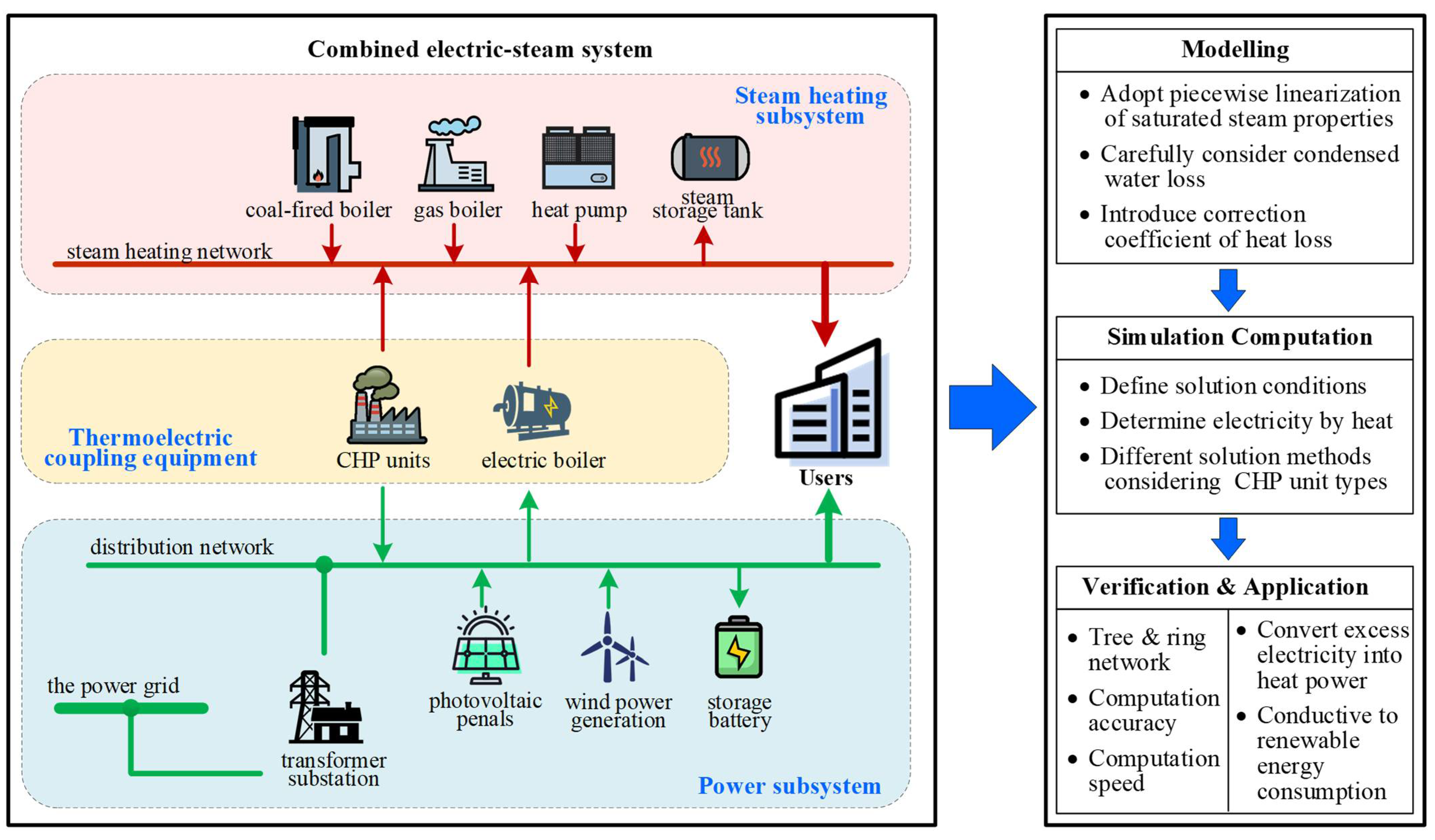
2. Simulation Model of CESS

As presented in Figure 1, a typical CESS consists of three parts: (1) power subsystem; (2) steam heating subsystem; and (3) thermoelectric coupling equipment. The cooperation between the power subsystem and the steam heating subsystem is realized through the thermoelectric coupling equipment. In order to construct the mathematical model of the CESS, models of the three key components are established first, and the three different components are then integrated to form the CESS model.

2.1. Simulation Model of the Power Subsystem

The steady-state mathematical model of the power system describes the system’s operational states and the power flow distribution. At present, research on the steady-state model of the power system and its computational methodology is already mature and commonly acknowledged and has been widely applied in the planning and dispatching of the actual power grid. For the power subsystem of IES, which may contain CHP units, photovoltaics, wind power, and other cogenerated equipment, the current model is still applicable. As a result, this paper adopts the traditional steady-state AC power flow equations as the mathematical model of the power subsystem. Equation (1) shows the traditional power flow equations in polar coordinates:

$$P_m+\mathbf{j}{Q}_m=U_m{\displaystyle \sum _{n=1}^{N_E}{U}_n}\left(G_{mn}-\mathbf{j}{B}_{mn}\right)\left(\cos {\delta }_{mn}+\mathbf{j}\sin {\delta }_{mn}\right) , \forall m,n\in E$$

(1)

where E is the set of all nodes in the power subsystem. N_E is the number of the nodes in the power subsystem. P_m and Q_m are the active power and reactive power injected into node m. U_m and δ_m are the voltage amplitude and phase angle of node m. δ_mn denotes the difference between δ_m and δ_n, namely δ_mn = δ_m − δ_n. j refers to the imaginary unit, which is a traditional practice in power systems to substitute the original mathematical symbol of the imaginary unit i, as i usually refers to the electric current in the power system. G_mn and B_mn are the real part and imaginary part of the mutual admittance between node m and node n (or the self-admittance of node m when m = n). The definitions of mutual admittance and self-admittance are detailed in [26].

Among the four state variables of node m (U_m, δ_m, P_m, and Q_m), two of them should be given in view of the feasibility of the power flow solution. According to the given variable types, the nodes/buses can be classified into PV buses (P_m and U_m is given), PQ buses (P_m and Q_m is given), and the slack bus (U_m and δ_m is given, usually only one slack bus for one system) [27].

2.2. Simulation Model of the Steam Heating Subsystem

2.2.1. Model Assumptions

Reasonable simplification and reformation are of great significance in the mathematical modeling process of a real physical system. Appropriate assumptions can help reach a balance between the simulation accuracy and computation complexity of a model [28]. To model the steam heating subsystem, the following assumptions are made:

(1) Curved pipelines are turned into straight pipelines of an equal length. Most of the actual steam pipelines are laid in bends. In order to simplify the calculation of the model, straight pipelines of the same length are used instead of curved pipelines. Segment linearization is adopted for pipes with a large curvature.

(2) The steam in the pipe is assumed as a one-dimensional steady-state flow [29]. Since the parameters of the steam at the same cross-section of the pipe have no significant differences, it is assumed that the steam parameters are uniformly distributed on the same cross-section. Changes only occur in the direction along the pipeline.

(3) The steam in the pipe is considered as a single-phase compressible fluid. In the process of steam transmission, condensed water is generated accompanied by a pressure loss and temperature drop. To prevent the water hammer effect caused by condensed water, steam traps are installed at intervals along the pipe to gather and drain the condensed water. As a result, the steam in the pipe is considered as a single-phase compressible fluid for modeling [30].

2.2.2. Pipeline Momentum Conservation Equations

The density, flow rate, pressure, and other parameters of steam change at different positions of the pipeline, so the dynamic process of the steam micro-element (a micro volume of steam) is analyzed to establish the precise model. Since the hot steam is assumed as a one-dimensional flow, changes only occur in the direction along the pipe. The x-coordinate axis is established along the pipe, taking the steam flow direction as the increasing x direction (unit: m). t denotes the time (unit: s). A denotes the cross-sectional area of the pipeline (unit: m²). Then, the volume of the steam micro-element can be expressed as $A\cdot dx$. P = P(x,t) denotes the steam pressure at position x and time t (unit: Pa).

According to the conservation of momentum, the momentum change in the steam micro-element equals the total impulse of all external forces exerted on the micro-element. The momentum conservation equation for unstable steam flow can be written as Equation (2): [15]

$$\frac{\partial (\rho u)}{\partial t}+\frac{\partial \left(\rho u^2\right)}{\partial x}+\frac{\partial P}{\partial x}+g\rho \sin \theta +\rho \frac{\lambda }{d}\cdot \frac{u^2}{2}=0$$

(2)

where ρ and u are the density (kg/m³) and flow velocity (m/s) of the steam micro-element. g is the acceleration of gravity (m/s²). θ is the angle between the pipeline and the horizon (rad). λ is the frictional resistance coefficient of the pipeline (dimensionless), which can be calculated by the Colelbrook–White equation. d is the inner diameter of the pipe (m).

In the momentum Equation (2), the first term is the inertia term, the second term is the convection term, and the fourth term is the gravity term. According to the model assumptions, the steam flow is considered to be in a constant steady flow. In this case, the three terms of inertia, gravity, and convection can be ignored, the specific reasons of which are as follows:

(1) In steady-state modeling, the steam is considered as a constant steady flow, so the steam parameters in the pipeline are independent of the time t and remain consistent at any time. Therefore, the inertia term can be ignored.

(2) From the engineering point of view, the convection term is meaningful only when the flow velocity is very high (close to the speed of sound) while the steam velocity in the steam heating system is generally 10–70 m/s [31], which is much smaller than the speed of sound. Thus, the convection term can be ignored.

(3) According to the physical parameters of the actual steam heating network, the gravity term can be ignored when the elevation difference of the pipe network is not large.

After ignoring the inertia, convection, and gravity terms, the steady-state momentum conservation equation of the steady-state steam flow can be obtained, as shown in Equation (3):

$$\frac{\partial P}{\partial x}+\frac{\lambda }{d}\cdot \frac{u^2}{2}\rho =0$$

(3)

where Q denotes the mass flow rate of steam (kg/s) and it has the following relationship with the other parameters, as shown in Equation (4):

$$Q=\rho uA$$

(4)

When Equation (4) is incorporated into Equation (3) and the steam flow velocity u is eliminated, then the steady-state differential momentum equation of the steam can be obtained, as shown in Equation (5):

$$dP+\frac{\lambda Q^2}{2d\rho A^2}dx=0$$

(5)

In Equation (5), the steam density ρ is a variable related to both pressure P and temperature T, which greatly increases the complexity of the equation. When the steam is saturated, the steam temperature T can be uniquely determined by the steam pressure P. Therefore, the steam density ρ can be regarded as just a function of pressure P. Using the relationship between ρ and P for saturated steam, the variable ρ in (5) can be eliminated. For saturated steam, when the steam pressure P is known, the density ρ can be obtained by looking up the corresponding table. However, for the convenience of code computation, the fitting relationship between the density and pressure of saturated steam is introduced, the selected form of which is piecewise linear fitting, as shown in Equation (6). Within each pressure range, the relative error of the fitting equation is within ±2%:

$$\rho =c_{1}P+c_2$$

(6)

where c₁ and c₂ are the fitting coefficients, and their values are shown in

Table 1. Values of the fitting coefficients for saturated steam density calculation.

Pressure Range (MPa)	c1 (×10−6 kg/(MPa·m3))	c2 (kg/m3)
0.10–0.32	5.2353	0.0816
0.32–0.70	5.0221	0.1517
0.70–1.00	4.9283	0.2173
1.00–2.00	4.9008	0.2465
2.00–2.60	4.9262	0.1992

.

Equation (6) is incorporated into Equation (5) and a differential equation without ρ is obtained. Because the variation of the flow rate Q along the pipeline is usually small enough to be ignored, the equation can be considered as a differential equation about P and x only. The obtained differential equation is integrated and an algebraic equation is obtained, as shown in Equation (7):

$$Q^2-\frac{1.2337d^5\cdot \left[c_1\left(P_{in}^2-P_{out }^2\right)+c_2\left(P_{in }-P_{out }\right)\right]}{\lambda \cdot L}=0$$

(7)

where L is the length of the pipe (m). P_in and P_out are the steam pressure at the entrance and exit of the pipeline, respectively (Pa).

Finally, regarding the influence of the local resistance loss in the pipeline, the flow efficiency factor e is introduced (dimensionless). When the pipeline is newly built, there is no local resistance caused by elbows and varying diameters, so the value of e is 1.00. When the pipeline is in good operating conditions, the value of e is 0.95. When the pipeline is in normal operating conditions, the value of e is 0.92. When the pipeline is in a very poor operating state, the value of e is 0.85. The steady-state momentum conservation equation of the pipeline after considering the local resistance loss is shown in Equation (8):

$$Q^2-\frac{1.2337d^5\cdot \left[c_1\left(P_{in}^2-P_{out}^2\right)+c_2\left(P_{in}-P_{out}\right)\right]}{\lambda \cdot L\cdot e}=0$$

(8)

Thus, the pipeline momentum conservation equations for the whole steam heating network can be expressed as:

$$Q_i^2-\frac{1.2337d_i{}^5\cdot \left[c_1\left(P_{in,i}^2-P_{out,i}^2\right)+c_2\left(P_{in,i}-P_{out,i}\right)\right]}{{\lambda }_i\cdot L_i\cdot e_i}=0 , i\in W$$

(9)

where W is the collection of all pipelines in the steam heating network. Q_i is the steam mass flow rate in the pipeline i, which can be substituted by the average value of the flow rate at the entrance and exit of the pipeline, as shown in Equation (10):

$$Q_i=\frac{1}{2}\left(Q_{in,i}+Q_{out,i}\right) , i\in W$$

(10)

where Q_in,i and Q_out,i are the steam flow rate at the entrance and exit of the pipeline i, respectively.

2.2.3. Nodal Mass Flow Conservation Equations

Based on Kirchhoff’s first law (or continuity theorem), the total steam mass flow injected into a node is equal to the total mass flow withdrawn from it. Therefore, the nodal mass flow conservation equations can be written as Equation (11):

$${\displaystyle \sum _j{Q}_{out,j}}-{\displaystyle \sum _k{Q}_{in,k}}+Q_{n,i}=0 , i\in V ,j\in W_{in,i} , k\in W_{out,i}$$

(11)

where Q_n,i is the injected steam flow rate at node i. W_in,i is the collection of all pipes flowing into node i and W_out,i is the collection of all pipes flowing out of it. For the N-node steam heating network, a total of N nodal mass flow conservation equations can be obtained.

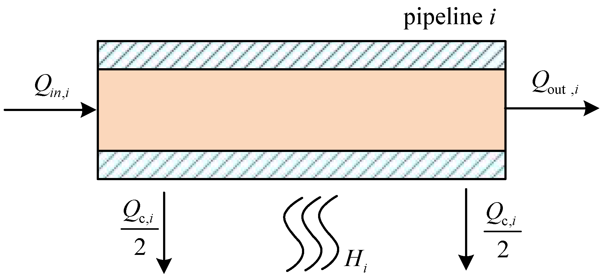
2.2.4. Pipeline Mass Flow Conservation Equations

Since the temperature difference between the transmitted steam and the ambient environment is normally higher than 100 °C, heat loss during the steam transmission process cannot be ignored. The heat dissipation leads to a steam temperature drop and even makes part of the steam condense into liquid water. In the model assumptions, it is assumed that the condensed water in the pipeline can be discharged by the steam traps along the way. It is supposed that the total mass flow of condensed water produced in pipeline i is Q_c,i (kg/s). The pipeline mass flow model is illustrated in Figure 2.

The pipeline mass flow conservation equations can be established from the conservation of mass, as shown in Equation (12):

$$Q_{in,i}=Q_{out,i}+Q_{c,i} , i\in W$$

(12)

where Q_in,i and Q_out,i are the mass flow rate at the beginning and end of the pipeline i (kg/s).

2.2.5. Pipeline Energy Conservation Equations

According to the conservation of energy, the change in the steam enthalpy along the pipeline should be consistent with the total heat dissipation loss. Thus, the energy conservation equations of the steam pipelines can be established, as shown in Equation (13):

$$Q_{in,i}{h}_{in,i}=Q_{out,i}{h}_{out,i}+Q_{c,i}{h}_{c,i}+H_i , i\in W$$

(13)

where h_in,i and h_out,i are the specific enthalpy (kJ/kg) of the steam at the beginning and end of the pipeline i, respectively. h_c,i is the specific enthalpy (kJ/kg) of the condensed water generated in the pipeline i. H_i is the total dissipation loss power (kW) during the steam transmission process in the pipeline i.

The specific enthalpy of saturated steam or saturated water can be obtained by looking up the table according to the known pressure P; however, this method is not suitable for code computation. For the convenience of model solving, a fitting formula is adopted to calculate the specific enthalpy. For the specific enthalpy of the steam at the beginning and end of the pipeline, the calculation formula is shown in Equation (14):

$$h=\frac{69722.19}{a_0+a_1{P}^{-0.5}+a_2{P}^{-1}+a_3{P}^{-1.5}+a_4{P}^{-2}+a_5{P}^{-2.5}+a_6{P}^{-3}}$$

(14)

where the unit of pressure P needs to be converted into MPa. a₀–a₆ are constant coefficients, the values of which are shown in [32]. The applicable range of Equation (14) is 0.40 MPa ≤ P ≤ 2.50 MPa and the relative error is within ±8.7 × 10⁻⁶.

The specific enthalpy of condensed water is calculated by Equation (15):

$$h_{c,i}=\frac{3704.12P_i^{0.6}}{1-222271P_i^{0.2}+7.55636P_i{}^{0.4}-1.476876P_i{}^{0.6}} , i\in W$$

(15)

where the unit of P_i still needs to be converted into MPa. The applicable range of Equation (15) is 0.40 MPa ≤ P ≤ 2.50 MPa, and the relative error is within ±2.4 × 10⁻⁵.

The heat dissipation loss is proportional to the length of the pipe and the temperature difference between the inside surface and the ambient environment of the pipe. The calculation formula commonly adopted in the existing literature is shown in Equation (16):

$$H_i=K_i{L}_i\left(T_i-T_a\right) , i\in W$$

(16)

where K_i is the comprehensive heat transfer coefficient of pipe i (KW/(m·K)), which is the heat dissipation of one meter of the pipeline per second when the temperature difference between the inside and the outside is 1 °C. L_i is the length of the pipeline i (m). T_i is the average steam temperature in the pipe i (K) and T_a is the ambient temperature outside the pipe (K).

The fitting formula between the temperature and pressure of saturated steam is shown in Equation (17):

$$T=202.7651P^{0.2148}-22.907$$

(17)

where T_i can be taken as the average value of steam temperature at the beginning and end of pipeline i, as shown in Equation (18):

$$T_i=101.38255\left(P_{in,i}{}^{0.2148}+P_{out,i}^{0.2148}\right)-22.907$$

(18)

For the calculation of K_i in Equation (16), the calculation method varies according to the laying mode of the pipeline. There are mainly three modes: overhead laying, direct buried laying, and pipe trench laying. The detailed calculation methods are given in [15].

However, Equation (16) is derived from pure theory and has a certain deviation from engineering practice. According to [33], due to the exposure of the tube drag, the weather has a great influence on the heat loss. As the pipeline is in direct contact with the pipe frame, part of the pipeline is exposed, meaning the pipe bracket is in a non-insulated state, which is equivalent to 1~2% of the pipeline being exposed. On sunny days, the heat dissipation loss will increase by 10–20%; on rainy days, the dissipation of the entire pipe network can even increase by 3–6 times. Therefore, the heat dissipation loss of the pipe network varies greatly with the weather conditions. This paper introduces a correction coefficient C_t on the basis of Equation (16) to correct the influence of weather and other factors on the heat dissipation loss, so that the calculated value is more consistent with reality. After the introduction of C_t, the calculation formula of heat loss power H is shown in Equation (19):

$$H_i=C_t{K}_i{L}_i\left(T_i-T_a\right) , i\in W$$

(19)

On sunny days, the value of C_t is suggested to be 1.3, taking various additional losses into account. When it is cloudy, C_t varies according to the weather conditions, and the value selection should be carried out reasonably based on the practical conditions and empirical data of each system.

Equation (19) is substituted into Equation (13) to obtain the final expression of the pipeline energy conservation equations, as shown in Equation (20):

$$Q_{in,i}{h}_{in,i}=Q_{out,i}{h}_{out,i}+Q_{c,i}{h}_{c,i}+C_t{K}_i{L}_i\left(T_i-T_a\right) , i\in W$$

(20)

2.2.6. Summary of the Control Equations for the Steam Heating Network

Based on the previous analysis, for a steam heating network with N nodes and M branches, a total of (3M + N) control equations can be obtained, including M pipeline momentum conservation equations, N nodal mass flow conservation equations, M pipeline mass flow conservation equations, and M pipeline energy conservation equations. The control equations of an N-node M-branch steam heating network are shown in Equation (21):

$$\left\{\begin{array}{l}{Q}_i^2-\frac{1.2337d_i{}^5\cdot \left[c_1\left(P_{in,i}^2-P_{out,i}^2\right)+c_2\left(P_{in,i}-P_{out,i}\right)\right]}{{\lambda }_i\cdot L_i\cdot e_i}=0 , i\in W\\ {\displaystyle \sum _j{Q}_{out,j}}-{\displaystyle \sum _k{Q}_{in,k }}+Q_{n,i}=0 , i\in V , j\in W_{in,i} , k\in W_{out,i}\\ Q_{in,i}=Q_{out,i}+Q_{c,i} , i\in W\\ Q_{in,i}{h}_{in,i}=Q_{out,i}{h}_{out,i}+Q_{c,i}{h}_{c,i}+C_t{K}_i{L}_i\left(T_i-T_a\right) , i\in W\end{array}\right.$$

(21)

2.3. Simulation Models of Thermoelectric Coupling Equipment

The thermoelectric coupling equipment plays an irreplaceable role of connecting the power system and the heating system in the CEHS. Typical thermoelectric coupling devices include CHP units, electric boilers, heat pumps, etc. The steady-state models of the CHP units and the electric boiler are introduced in this section.

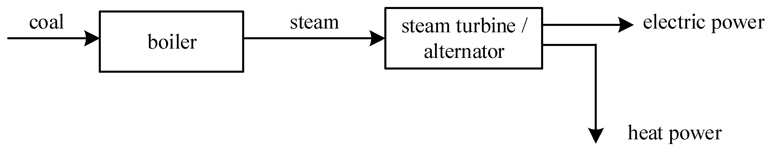
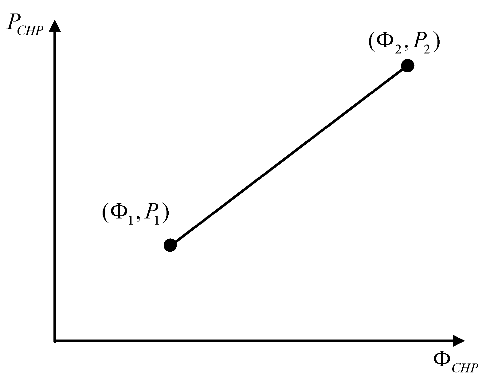
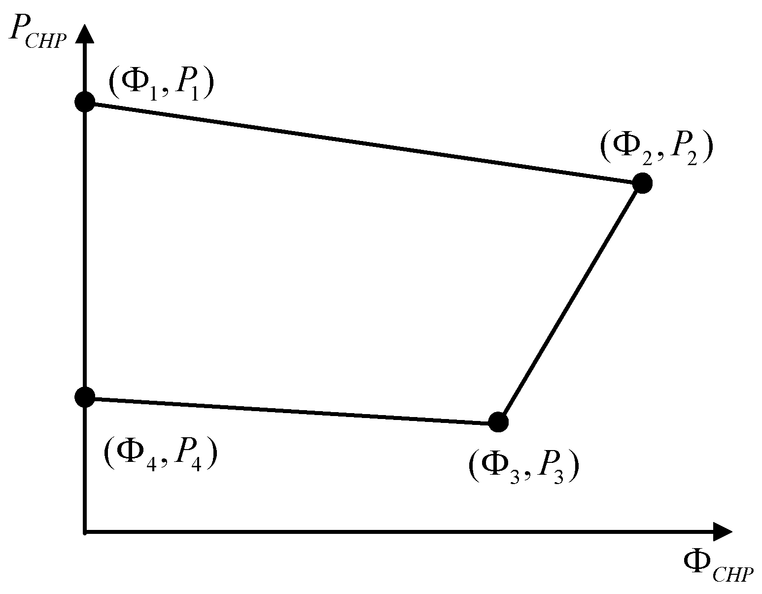
2.3.1. Simulation Model of CHP Units

CHP units can simultaneously supply electricity and heat by burning coal or natural gas. According to the different usage of the original steam generated by coal or natural gas, CHP units can be divided into back-pressure units and extraction condensing units. The condensing units can be further divided into single-extraction units and double-extraction units according to the heating mechanisms. Regarding the different mechanisms of different types of CHP units, their models are also different.

• Back-pressure unit

The schematic diagram of the back-pressure unit is shown in Figure 3. Since there is no condenser, all steam generated by the boiler expands in the steam turbine to generate electricity. Then, the waste heat is collected for heating. The thermal efficiency is relatively high due to full utilization of the waste heat [34].

Since all the exhaust steam of the back-pressure units is used for heating, it can be considered that the generated electric power P_CHP is basically linear with the thermal power Φ_CHP, as shown in Equation (22):

$$P_{CHP}=K_{CHP}{\Phi }_{CHP}$$

(22)

where P_CHP and Φ_CHP are the electric power and thermal power produced by the CHP unit. K_CHP is the heat-to-power ratio, namely the ratio of the thermal power to the electric power.

Equation (22) can be transformed into the form of a constant heat-to-power ratio, as shown in Equation (23):

$$\frac{{\Phi }_{CHP}}{P_{CHP}}=K_{CHP}$$

(23)

The electrothermal characteristic diagram of the back-pressure unit is depicted in Figure 4.

2.

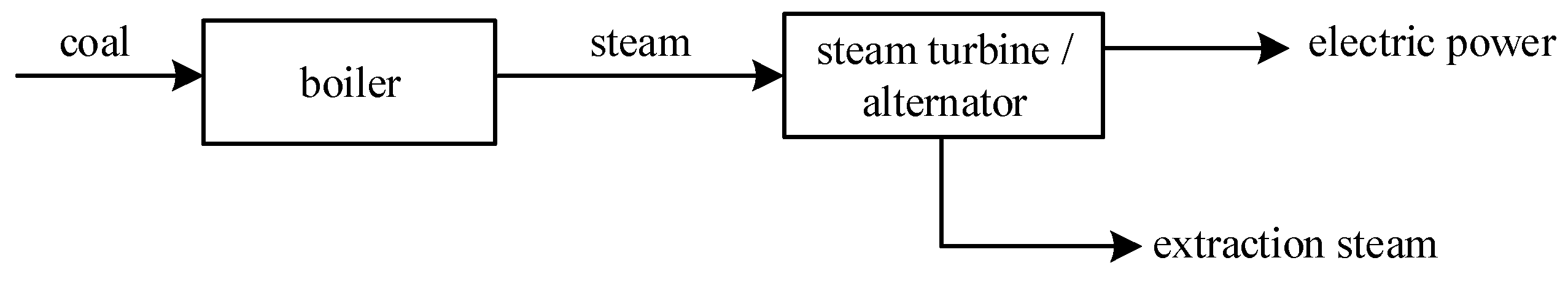
Extraction condensing unit

For the extraction condensing unit, part of the steam entering the steam turbine is extracted for the heat supply while the remaining part continues to expand in the turbine to perform work for power generation. The working mechanism is shown in Figure 5.

As the volume and pressure of the steam extracted for heating are adjustable, the output electric power and thermal power of the extraction condensing unit have more room for adjustment. For the extraction condensing unit, part of the steam is extracted for heating and the remaining part continues to generate electric power, so there is also a certain coupling relationship between its output electricity power and thermal power. The electrothermal characteristic diagram of the extraction condensing unit is shown in Figure 6.

From Figure 6, the coupling relationship between the electric power P_CHP and the thermal power Φ_CHP of the extraction condensing unit can be written as Equation (24):

$$\left\{\begin{array}{l}{P}_{CHP}={\displaystyle \sum _{i=1}^4{\alpha }_i}{P}_i\hfill \\ {\Phi }_{CHP}={\displaystyle \sum _{i=1}^4{\alpha }_i}{\Phi }_i\hfill \end{array}\right., where{\displaystyle \sum _{i=1}^4{\alpha }_i}=1,0\le {\alpha }_i\le 1$$

(24)

where (P_i, Φ_i) corresponds to the four boundary points in Figure 6. For the extraction condensing unit, the heat-to-power ratio is variable within a certain range.

2.3.2. Simulation Model of the Electric Boiler

The electric boiler is also one of the key coupling devices in CEHS, which often serves as a supplementary heat source for peak-shaving. It usually operates during nighttime in winter when the heat load is high but the electric load is low. By utilizing surplus electricity for heat production, the electric boiler is able to cut the peak of the heat load and fill the valley of the electricity load, thereby improving the operating efficiency and stability of the entire system. This creates more possibilities for the access of renewable energy sources such as photovoltaics and wind power.

A fixed peak-shaving ratio model is adopted as the simulation model of the electric boiler. The peak-shaving ratio refers to the ratio of the peak-shaving heat load borne by the electric boiler to the total heat load at the same node, and its expression is shown in Equation (25):

$$K_{EB}=\frac{{\Phi }_{EB}}{{\Phi }_{total}}$$

(25)

where K_EB is the peak-shaving ratio. Φ_EB is the peak-shaving heat power provided by the electric boiler. Φ_total is the total heat load of the node where the electric boiler is installed.

3. Simulation Computation of CESS

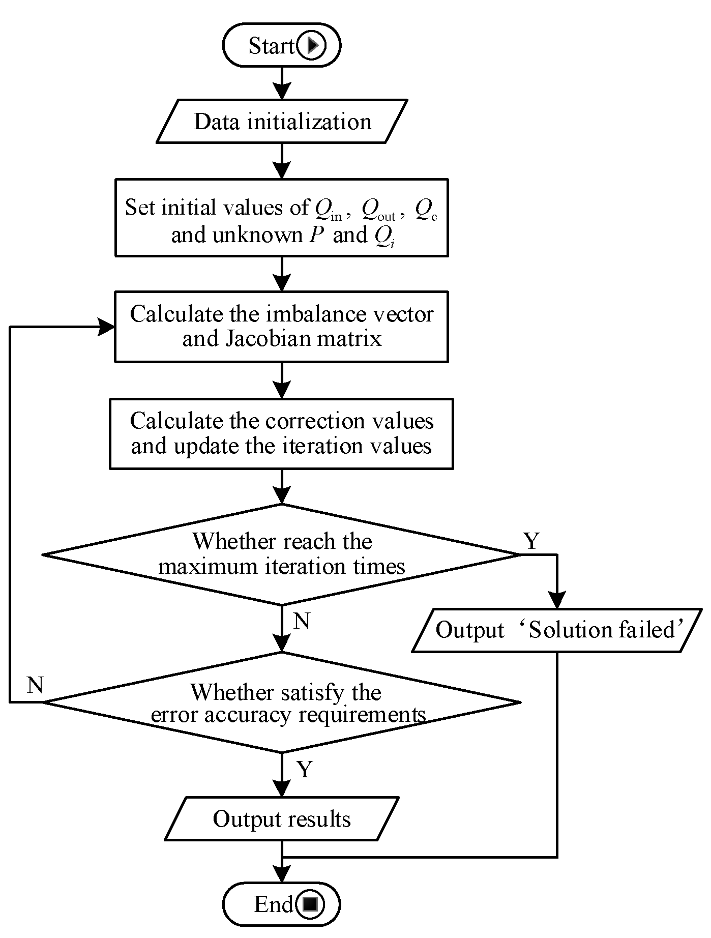
3.1. Computation of the Steam Heating Subsystem

3.1.1. Solution Conditions

To solve the simulation model of the steam heating subsystem established in Section 2, the following known conditions under stable operation are given.

(1) For any node in the system, one of the two variables, node pressure and node injection flow, should be given and the other is unknown.

(2) The pressure of at least one node in the entire system is known, and the node is generally at the heat source. When the output steam flow of the heat source does not reach the maximum limit, it usually works at the mode of constant output steam pressure and variable output flow. When the heat source runs at full capacity, the output flow is constant, and the output steam pressure is variable.

(3) Usually, at heat users and intermediate nodes, the injected steam flow is known and the steam pressure is unknown.

(4) The topological structure of the steam pipe network and all the pipeline parameters are given.

(5) The ambient temperature of the steam pipeline is given.

3.1.2. Establishment of the Equations and Solution

For a steam heating network with N nodes and M branches, there are a total of (3M + N) network control equations, as shown in

Table 2. Control equations of an N-node and M-branch steam heating network.

Control Equations	Quantity
Pipeline momentum conservation equations	M
Nodal mass flow conservation equations	M
Pipeline mass flow conservation equations	M
Pipeline energy conservation equations	N

.

The mathematical expressions of the (3M + N) control equations are shown in Equation (26):

$$\left\{\begin{array}{l}{Q}_i^2-\frac{1.2337d_i{}^5\cdot \left[c_1\left(P_{in,i}^2-P_{out,i}^2\right)+c_2\left(P_{in,i}-P_{out,i}\right)\right]}{{\lambda }_i\cdot L_i\cdot e_i}=0 , i\in W\\ {\displaystyle \sum _j{Q}_{out,j}}-{\displaystyle \sum _k{Q}_{in,k }}+Q_{n,i}=0 , i\in V , j\in W_{in,i} , k\in W_{out,i}\\ Q_{in,i}=Q_{out,i}+Q_{c,i} , i\in W\\ Q_{in,i}{h}_{in,i}=Q_{out,i}{h}_{out,i}+Q_{c,i}{h}_{c,i}+C_t{K}_i{L}_i\left(T_i-T_a\right) , i\in W\end{array}\right.$$

(26)

In the network, the quantities to be determined are Q_in, Q_out, and Q_c of the M pipelines, and the node pressure P or node injection flow Q_i of the N nodes. Thus, there are a total of (3M + N) unknowns, as shown in

Table 3. Unknowns of an N-node and M-branch steam heating network.

Unknowns	Quantity
Qin	M
Qout	M
Qc	M
P or Qi	N

.

All the (3M + N) unknowns can be solved uniquely through the (3M + N) simultaneous equations. Observing Equation (26), it is apparent that the network control equations are a set of nonlinear equations. In engineering practice, the topology of the steam heating network is generally simple, and the number of nodes or pipes is relatively small, so the Newton Raphson method is an efficient way to solve the nonlinear equations. The flowchart for solving the simulation model of the steam heating subsystem is shown in Figure 7.

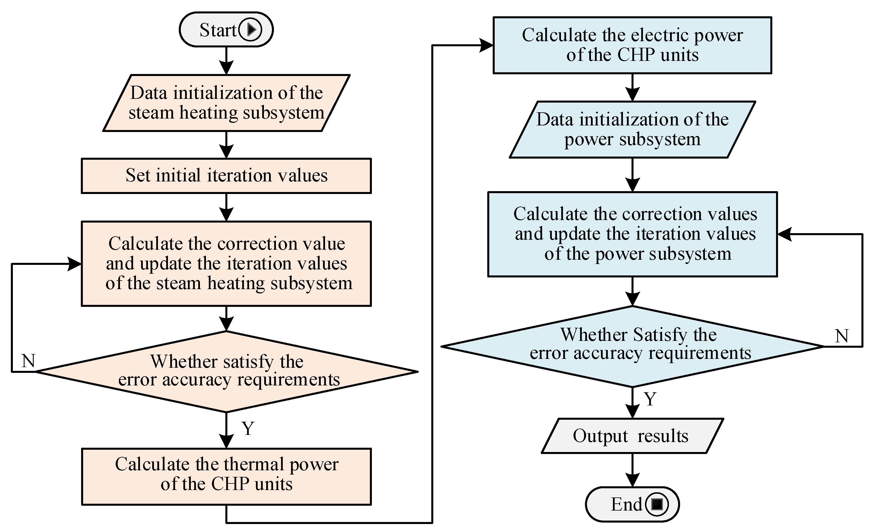
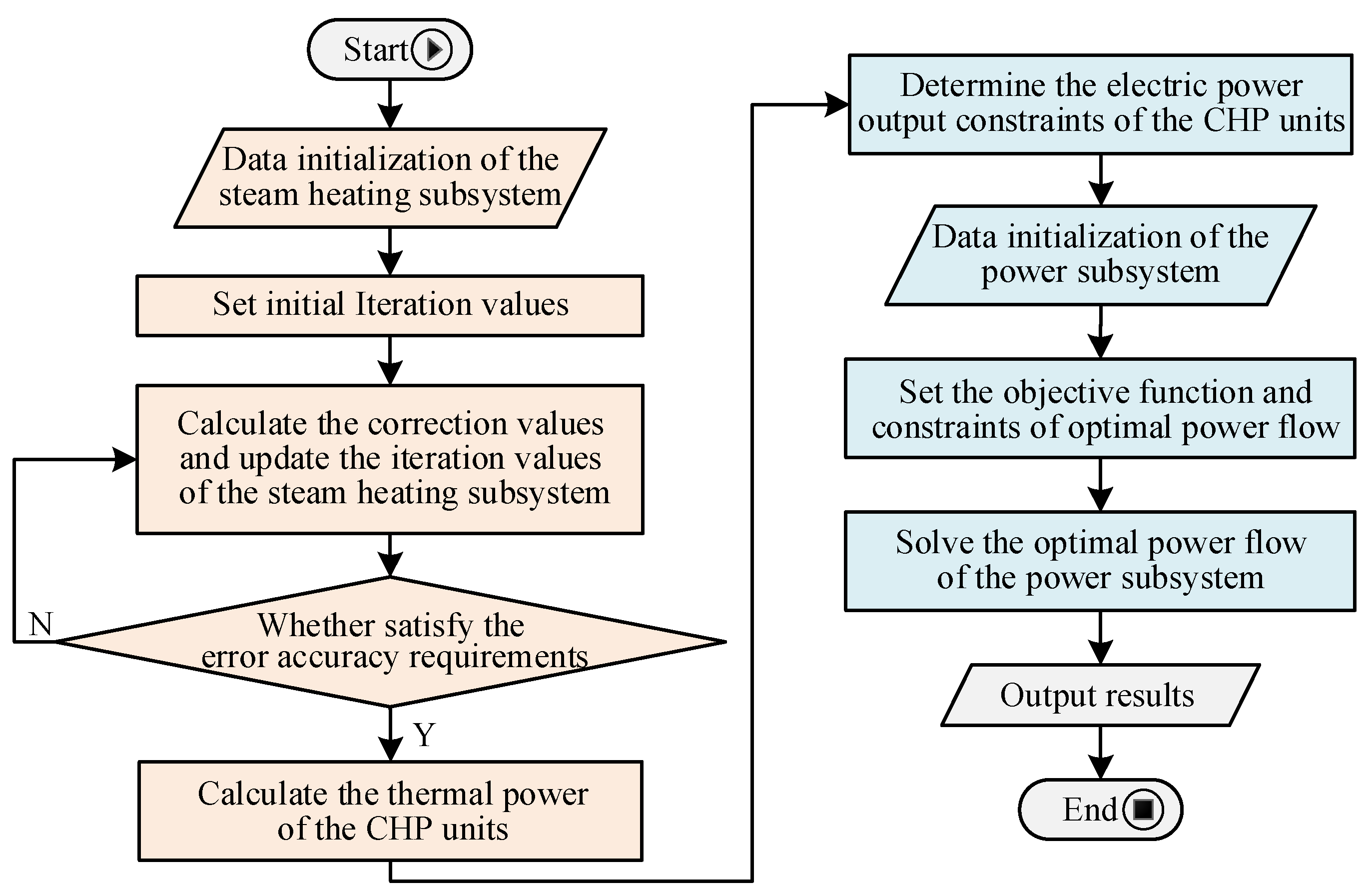
3.2. Computation of CESS

The characteristics of the coupling devices will determine the correlation degree between the power subsystem and the steam heating subsystem, so the best computation method will differ according to the type of thermoelectric coupling equipment. The following context provides two computation frameworks of the CESS with two typical types of CHP units.

3.2.1. Back-Pressure Units Only

For the back-pressure unit, its electric power is proportional to the heating power; that is, the heat-to-power ratio is fixed. Considering the generally simpler topology and fewer heat sources of the steam heating subsystem and the larger scale and stronger adjustability of the power subsystem, the operation mode of ‘power determined by heat’ is usually adopted. Under this mode, the output heat power of the back-pressure unit is firstly determined according to the heat load, and then the output electric power is obtained through the fixed heat-to-power ratio.

Under the ‘power determined by heat’ operation mode, the decoupling between the steam heating subsystem and the power subsystem can be completely realized. When the heat load of the steam heating subsystem is known, the computation of the steam network can be carried out first and the output heat power of each heat source (including the CHP unit) can be obtained. Then, the output electric power of the back-pressure unit can be calculated by the fixed heat-to-power ratio, which is a known condition for the power subsystem. After, the power flow calculation is performed on the power subsystem. It is precisely because of the decoupling between the heating subsystem and the power subsystem that the simulation computation of the whole CESS can be simplified. The computation framework is shown in Figure 8.

3.2.2. Containing Extraction Condensing Units

Since the heat-to-power ratio of the extraction condensing unit is not a constant and can be adjusted within a certain range, when the combined system contains the extraction condensing unit, it is impossible to directly determine the output electric power of the unit by means of “power determined by heat”. It can be seen from Figure 4 that the electrothermal characteristic of the back-pressure unit is a straight line. When the thermal power is known, its electric power can be uniquely determined. Differently in Figure 6, the electrothermal characteristic of the extraction condensing unit is a two-dimensional area, so the power supply is unable to be uniquely determined when the thermal power is known. In this case, the optimal power flow problem is involved in the computation process. The computation framework of CESS with an extraction condensing unit is shown in Figure 9.

4. Case Verification and Analysis

In this section, the proposed model of the steam heating subsystem is firstly verified on both tree and ring networks. Meanwhile, comparisons are carried out with the commonly used model in terms of the computation accuracy and speed. Then, the proposed CESS simulation approach is applied to a CESS case with back-pressure units and electric boilers, aiming to analyze the advantages of electric boilers for promoting renewable energy consumption.

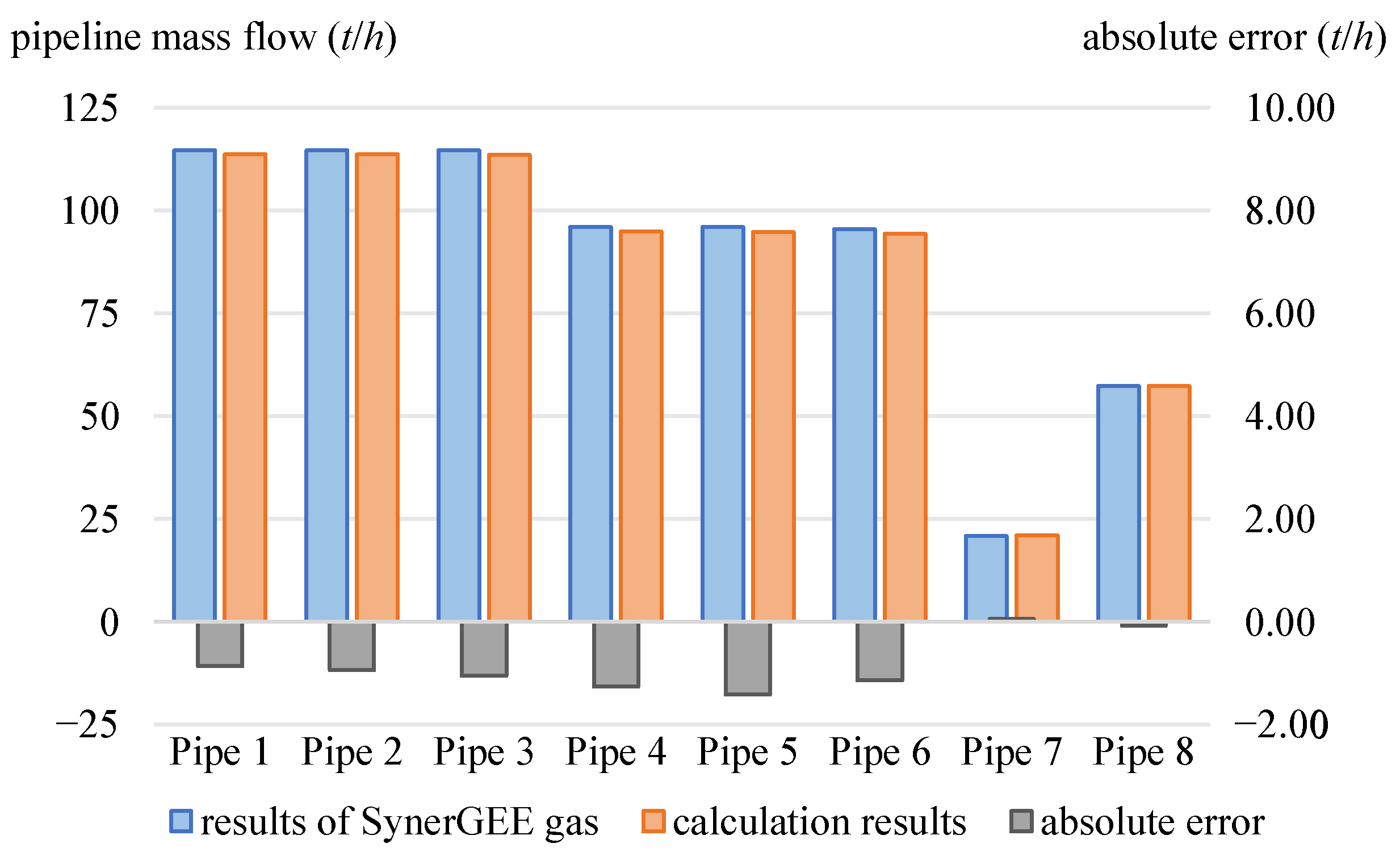
4.1. Case Verification of the Steam Heating Subsystem

The case verification of the steam heating subsystem is carried out on a nine-node double-heat-source tree network and a nine-node double-heat-source ring network, respectively.

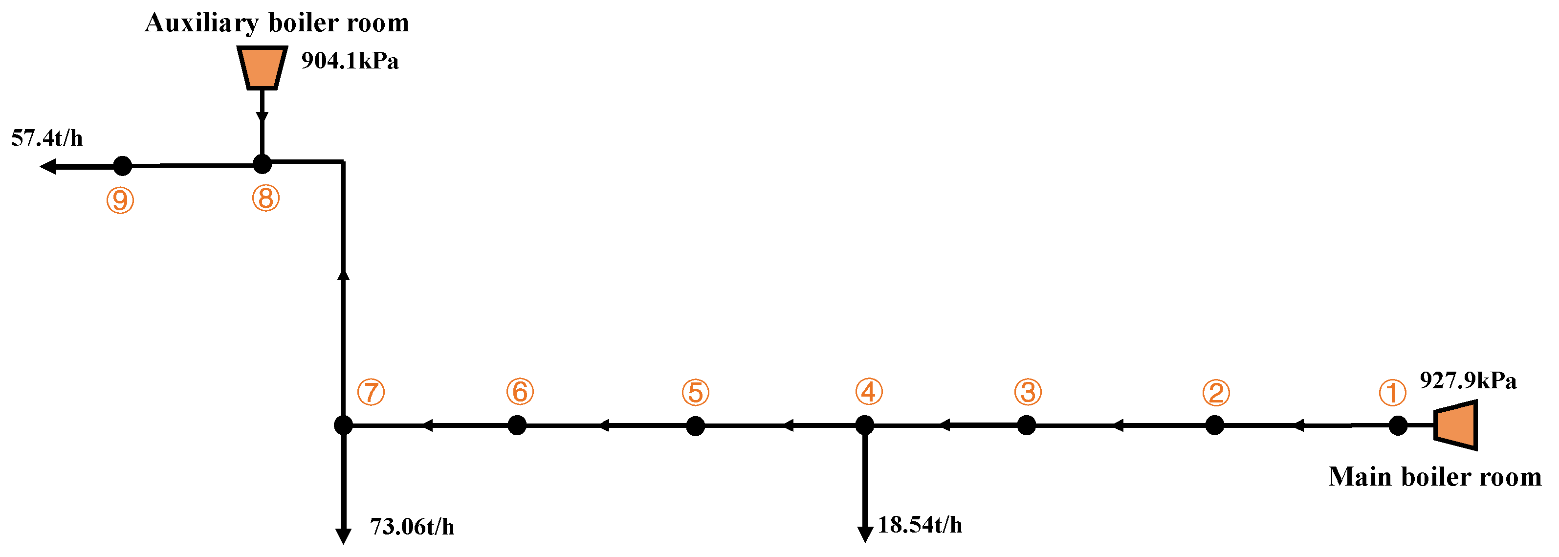
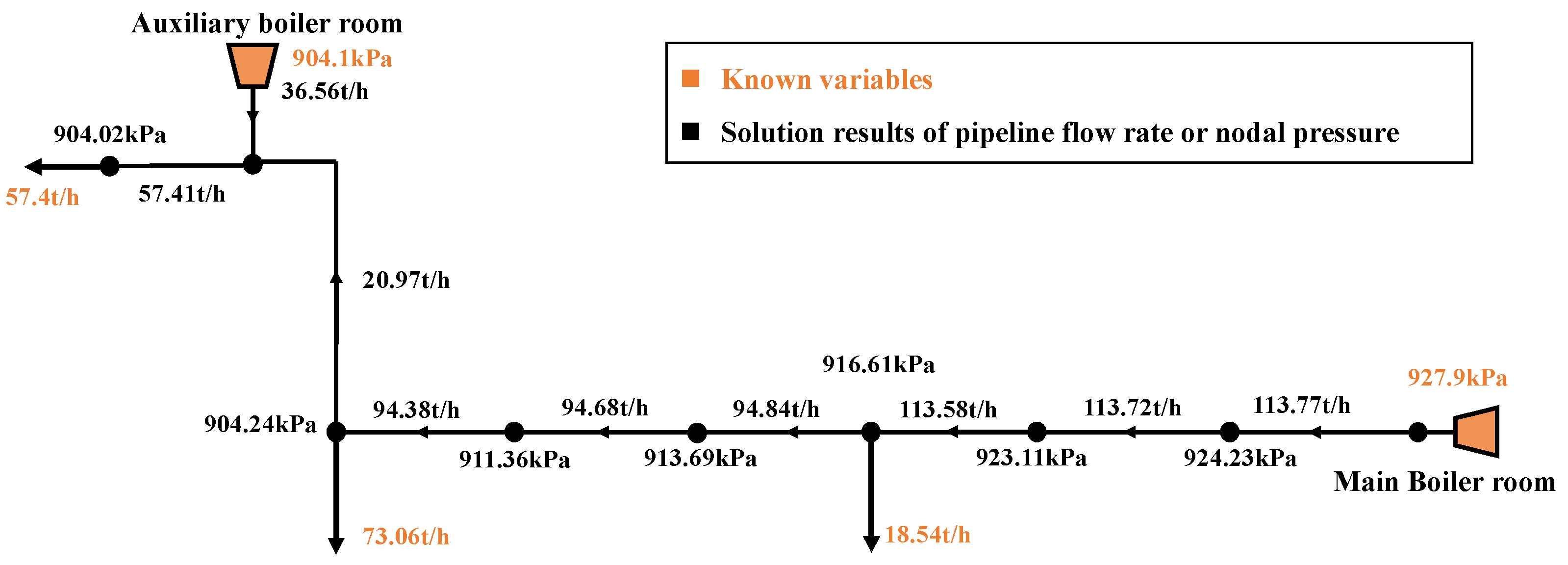
4.1.1. Nine-Node Double-Heat-Source Tree Network

For the tree network verification, the case is built based on the data of District 1 of the Tianjin Airport Industry Park (data is available in [15]). The case is a nine-node double-heat-source simplified tree network, considering the other districts of the park as equivalent heat loads to the corresponding node. The equivalent network is shown in Figure 10, where node 1 and node 8 are connected to the main boiler room and the auxiliary boiler room, respectively, and no closed loop exists in this network. The main boiler room at node 1 serves as the main heat source, with a capacity of 300 t/h, and the auxiliary boiler room at node 8 serves as the peak-shaving boiler. See Appendix A for the detailed parameters.

The heat load data at 10 A.M. on 15 January 2010 is adopted. The pressure of node 1 and node 8, where the main boiler room and the auxiliary boiler room are located, is given as constants. The correction coefficient C_t is determined as 1.3. After four iterations of computation, the error converges to the preset precision. The calculated result is shown in Figure 11.

SynerGEE gas is a relatively accurate commercial simulation software of the thermal system [15]. Using the simulation results of SynerGEE gas as a benchmark, flow verification of the proposed steam network model is carried out. Figure 12 compares the calculation results of the pipeline flow obtained by the proposed model and SynerGEE gas. The absolute error is within 1.6 t/h and the relative error is within 1.5%, indicating that the accuracy of the proposed model is high and can fully meet the simulation requirements.

Moreover, it is found that the total condensate volume of the 8 pipelines is 1.3885 t/h while the data provided by SynerGEE gas is 1.310 t/h. The relative error is 6% within the acceptable range. It is also obtained that the network will produce a total of 0.2779 kg condensed water per meter per hour on sunny days. This is consistent with the statistical data showing that an average of 0.30 kg condensed water is generally produced per meter per hour, under the condition that the pipe insulation layer is effective, the external environment temperature reaches 10 °C, and the steam pressure in the pipe reaches 0.6 [35].

4.1.2. Performance Comparison of Steam Heating Network Models

In order to better verify the superiority of the proposed steam heating network model, comparisons are made with a common existing model of the steam network in [11]. Based on the nine-node double-heat-source tree network, the calculation results of the two models are shown in

Table 4. Comparison of the solution results of the steam heating network model.

Results of SynerGEE Gas	Model in This Paper		Model in [11]
	Pipeline Flow (t/h)	Relative Error	Pipeline Flow (t/h)	Relative Error
114.6	113.589	0.91%	112.4	1.91%
114.6	113.527	0.96%	112.4	1.91%
114.6	113.427	1.05%	112.4	1.91%
96.09	94.7126	1.43%	93.90	2.28%
96.09	94.5772	1.57%	93.90	2.28%
95.52	94.3206	1.26%	93.90	1.70%
20.91	20.9516	0.20%	20.84	0.33%
57.47	57.4043	0.11%	57.40	0.12%
Maximum relative error	-	1.57%	-	2.28%
Iteration times	4	-	10	-
Solution time	1.32	-	333,281.63	-

.

According to the simulation results of SynerGEE gas, the maximum relative error of the proposed model is 1.57%, which is slightly smaller than that of the model in [11]. Both models can meet the accuracy requirements for simulation while the model in this paper has a slightly higher accuracy. Moreover, the proposed model has a significant advantage in computation speed, as the iteration times and solution time are much lower than those of the model in [11]. This is because the proposed model uses piecewise linear fitting to calculate the steam parameters, instead of using the accurate but complicated formulas provided by IAPWS-IF97, which largely accelerates the computation process.

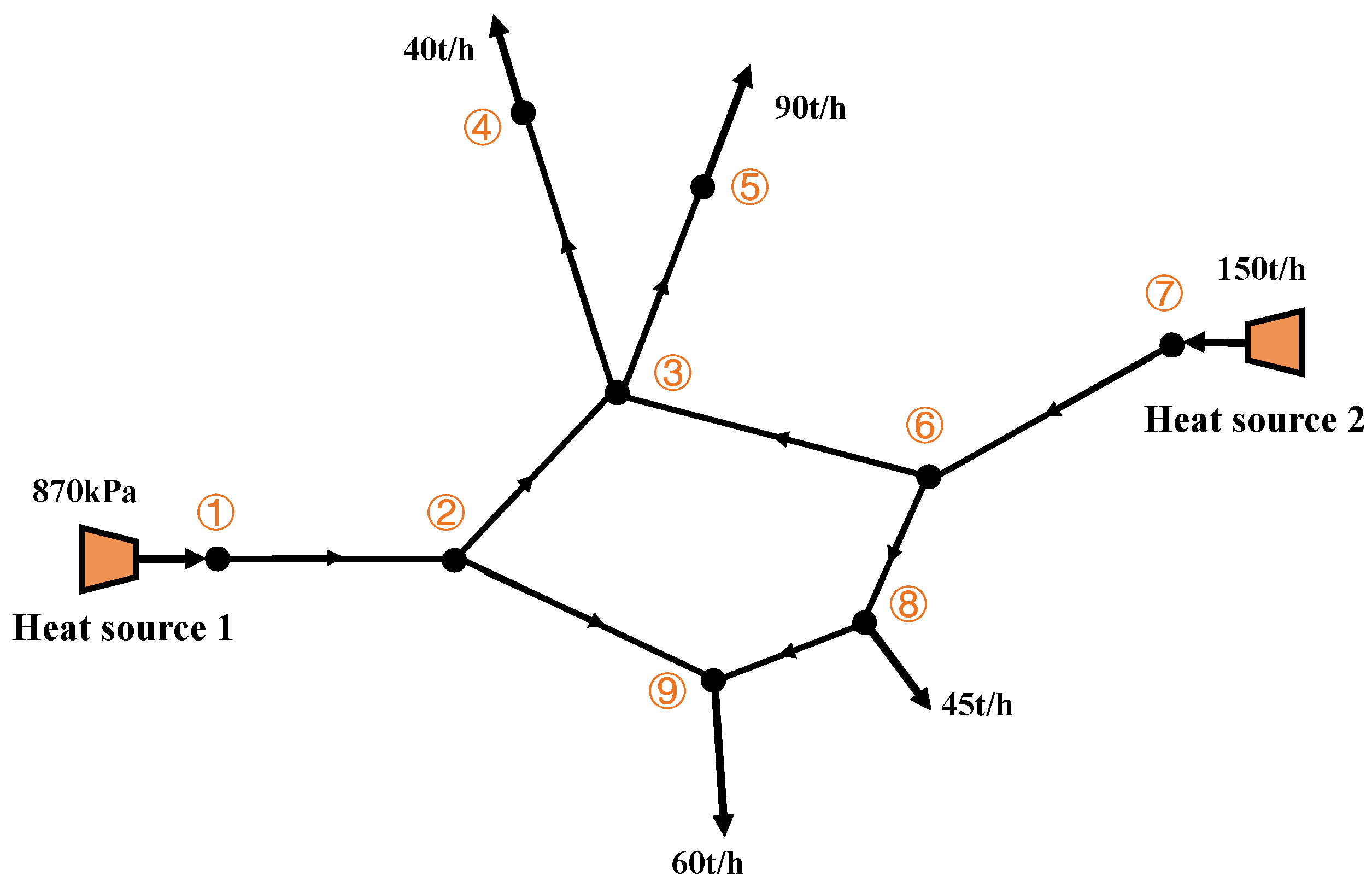
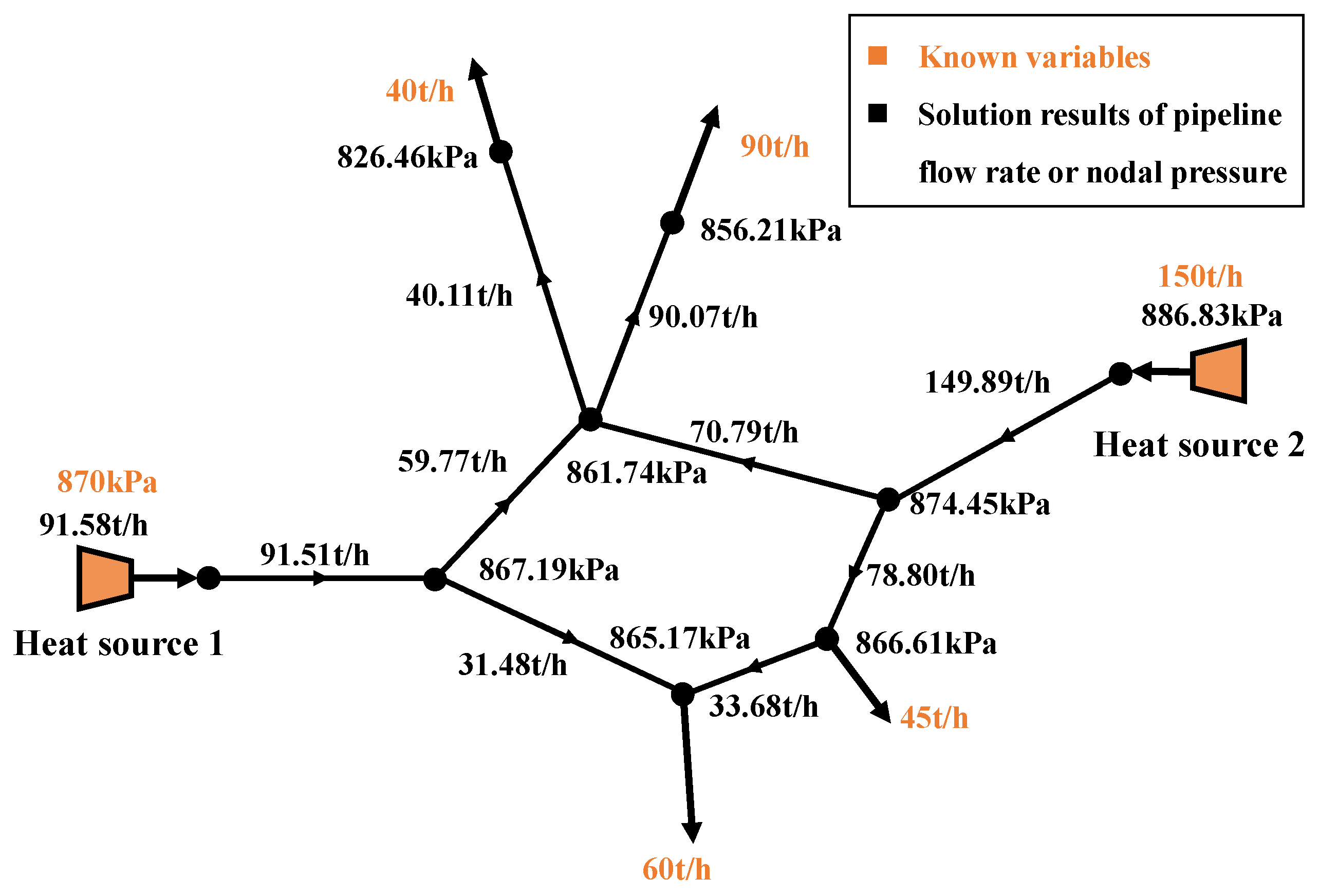
4.1.3. Nine-Node Double-Heat-Source Ring Network

The proposed steam network model is applicable to both the tree and ring network. In this section, a ring network case is studied based on the proposed methodology. Figure 13 presents a nine-node double-heat-source network with a single closed loop. The heat load of each node is marked out. The two heat sources are connected to node 1 and node 7, respectively. When operating, heat source 2 always supplies steam at a flow rate of 150 t/h while heat source 1 controls its pressure to be constant at 870 kPa. See Appendix A for the other parameters of the network.

The model can converge to the required accuracy after four iterations and the calculation results are shown in Figure 14. The pipeline flow rate, node pressure, and supply parameters of each heat source are marked.

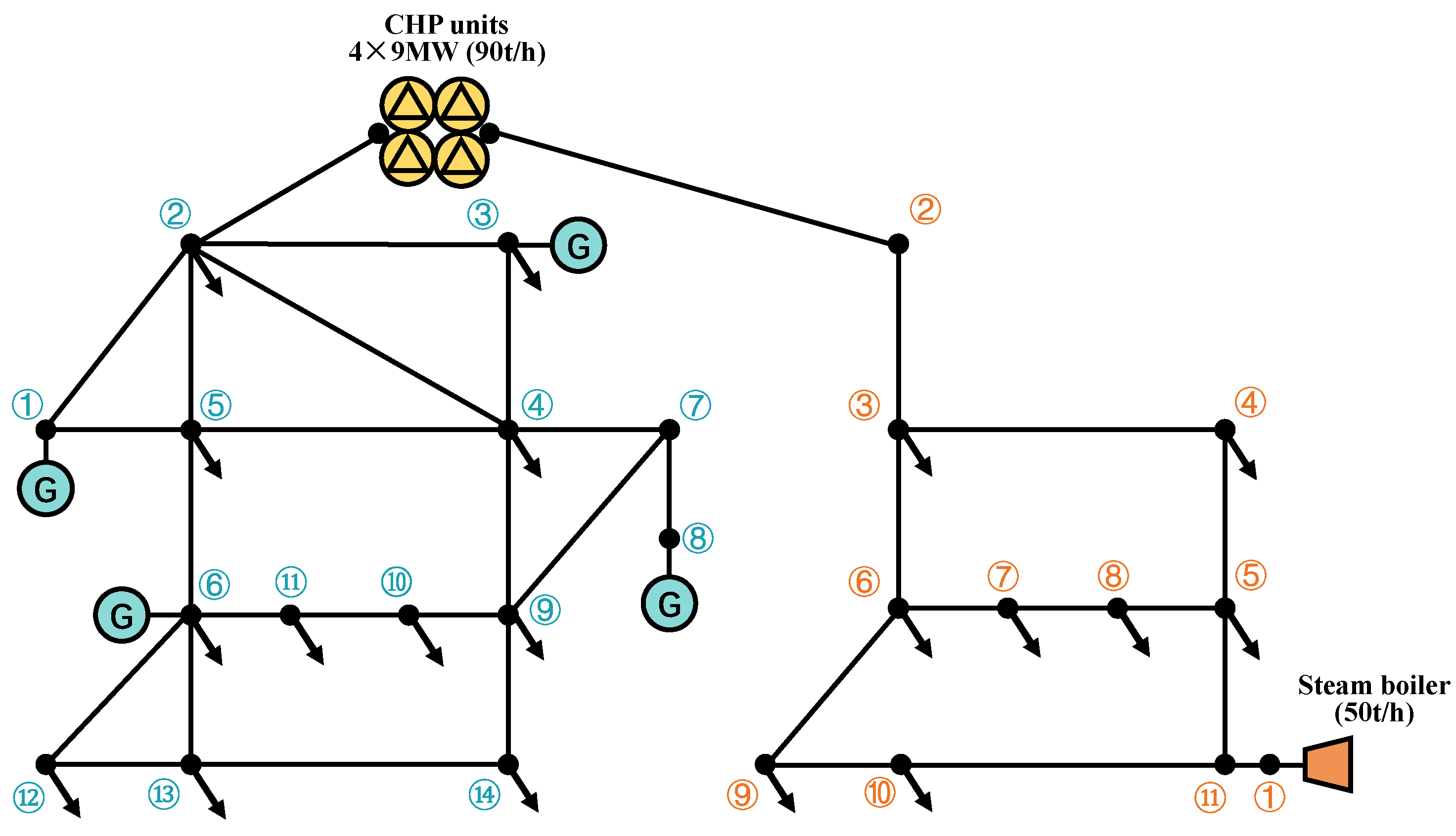
4.2. Case Analysis of CESS

In this section, a CESS case is selected for simulation analysis, and the coupling influence of electric boilers on the renewable energy consumption is examined.

4.2.1. Network Structure and Parameters

The CESS to be analyzed in this section is shown in Figure 15. The nodes of the power subsystem are marked in blue while the nodes of the steam heating subsystem are marked in orange. The power subsystem is based on the IEEE14 power system, which contains five generators, with node 1 being the slack bus. The steam heating subsystem is an 11-node double-loop network, whose structure is designed based on the power subsystem. This is because the positions of the heat users and electric users in the industrial scenario are usually consistent. A steam boiler with a capacity of 50 t/h is connected to node 1. The two subsystems are connected through the CHP units at their respective node 2. With reference to the product parameters of Qingdao Jieneng Steam Turbine Group Co., Ltd. (Qingdao, China), the CHP units are selected as a set of four back-pressure units, each with a capacity of 9 MW, and the total maximum steam output is 90 t/h. When the CHP units cannot satisfy all the heat load when supplying maximum heat power, the steam boiler at node 1 will work as a supplementary heat source and provide the remaining heat power. See Appendix A for the detailed parameters of the coupling system.

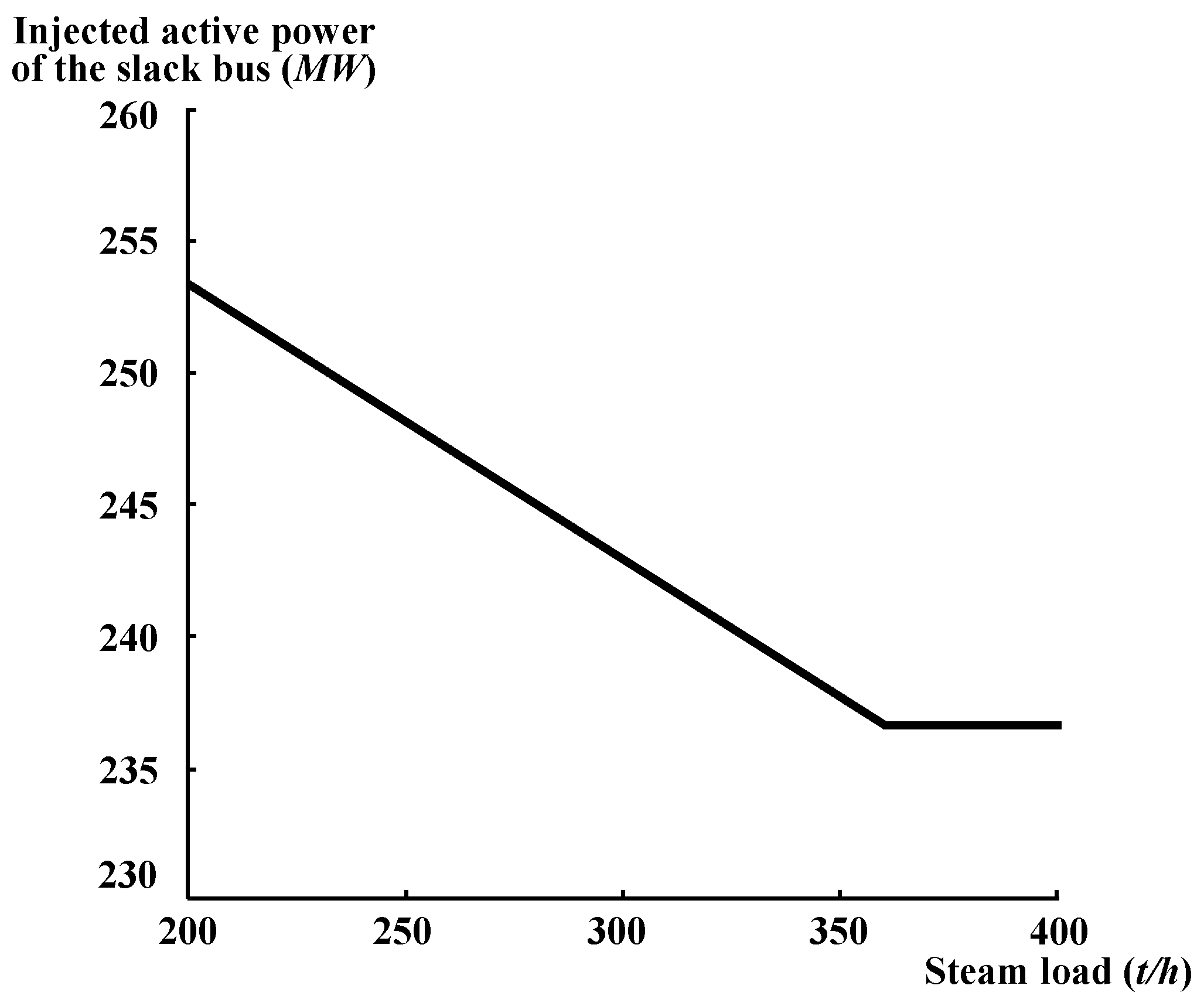
4.2.2. Simulation Computation

Since the network only contains back-pressure units, decoupling can be completely realized between the two subsystems. Under the “power determined by heat” mode, computation of the steam subsystem is carried out before the power subsystem. Although the computation process is decoupled, the two subsystems still function on each other through thermoelectric coupling devices. Changes in the heat load will finally influence the power injected into the slack bus. Analysis is carried out through the following example.

Figure 16 shows the change in the injected active power of the slack bus when the steam heating load gradually increases from 200 to 400 t/h. Change in the line can be divided into two stages.

Stage 1: In the beginning, when the heat load increases, the output heat power of the CHP units increases as well. As the heat-to-power ratio of the back-pressure unit is constant, its electric power also increases accordingly. When the electric load remains unchanged, the injected active power of the slack bus will decrease continuously in order to balance the generation and the load.

Stage 2: When the output of the CHP units reaches the upper limit, the output heat and electric power will stay constant. Then, the injected active power of the slack bus will also remain unchanged when the electric load remains the same. On this occasion, the remaining heat power will be supplied by the steam boiler at node 1.

4.2.3. Impacts of Electric Boilers on Renewable Energy Consumption

Uncontrollability and randomness are the main factors restricting the consumption of renewable energy. A large amount of renewable energy will cause an energy consumption problem since the electric power network needs an instantaneous balance between the generation and the load demand. In CEHS, electric boilers and CHP can dynamically adjust the electric load and generation and transfer the surplus electricity to heat for a certain period. CEHS is especially feasible and applicable for areas with abundant wind resources and a large heat load.

Generally, the wind power output is larger during the night than in the daytime, which is the opposite trend to the electricity load. This will lead to an imbalance between electric generation and consumption. On the contrary, for the heating network, the heat load is relatively constant. For CEHS, if the electric boiler is put into operation at night, it can play the role of cutting the peak of the heat load and filling the valley of the electric load. The electric boiler consumes surplus electric energy for the steam heating supply, which works as an additional load for the power subsystem and a supplementary heat source for the heating subsystem. Based on the proposed simulation method, the peak-shaving function and the benefits of electric boilers for renewable energy consumption are discussed in this section.

The conditions at 12:00 A.M. and 12:00 P.M. are selected for calculation and comparison. It is considered that the electric load at night drops to 50% of that in the daytime and the heat load drops to 83%. The load of each node is reduced by an equal proportion. Under such conditions, the total heat and power loads in the day and at night are shown in

Table 5. Heat load and power load of the coupling system.

	12:00 A.M.	12:00 P.M.
Power load	259 MW	129.5 MW
Steam heating load	384 t/h	318.7 t/h

.

It is considered that the electric boiler is not used during the day and is put into operation at night, especially at node(s) with higher heat loads. The peak-shaving ratio K_EB of the electric boiler is 0.4. For the convenience of the analysis, it is considered that the output power of the electric generators (except the balance unit) remains unchanged all the time, and the load fluctuations of the power subsystem are all borne by the balance unit. In this way, the change in the injected active power of the slack bus can directly indicate the change in the load of the power subsystem.

Based on the proposed simulation approach, the injected active power of the slack bus in the day and at night can be calculated, respectively, and the peak-valley difference of the slack bus.

Table 6. Comparison of the results when putting electric boilers into operation.

Position of Working Electric Boiler(s)	Injected Active Power of the Slack Bus/MW		Peak-Valley Difference/MW	Percentage Change of Peak-Valley Difference
	Day	Night
None	236.31	100.52	136.09	-
Node 4	236.31	116.78	119.83	−11.95%
Node 4 and Node 11	236.31	131.98	104.63	−23.12%
Node 3, Node 4, and Node 11	236.31	142.98	93.63	−31.20%

shows the simulation results when different numbers of electric boilers are put into operation.

Observing the data in Table 6, it can be seen that when the number of electric boilers operating at night increases, the injected active power of the slack bus at night also increases. Therefore, the peak-valley difference of the slack bus decreases, which can reduce the fluctuation of the active power supply of the balance unit. Especially when all the electric boilers at node 3, 4, and 11 operate, the peak-valley difference can be reduced by up to 31.20%.

In summary, the introduction of the electric boiler is able to reduce the load volatility of the power system. Since the load in the power system is partly increased by the electric boilers during a light load, it provides an effective solution to address the intermittency and volatility of renewable energy, especially wind power consumption.

5. Conclusions

This paper proposed a novel simulation approach for CESS, which can balance the simulation accuracy and speed. The major conclusions are summarized as follows.

(1) To address the complexity and inaccuracy in traditional steam network simulation, the piecewise linear fitting method and the heat loss correction coefficient were adopted to establish a high-precision and high-speed model of the steam heating subsystem. Results showed that the relative error of the pipeline flow was within 1.5%, which is slightly better than the traditional method. The computation speed was significantly improved, with the simulation time shortened to 0.479%.

(2) With consideration of the mainstream CHP units, two computation methodologies for back-pressure units and extraction condensing units were proposed, respectively. The distinct operation characteristics of the two types of CHP can be accurately simulated.

(3) To explore the application scenario of the proposed simulation approach, the renewable energy consumption capacity of a CESS with high penetration of wind energy was simulated and evaluated. It was found that the CESS can reduce the volatility of the grid load by up to 31.20% through the adoption of electric boilers.

References

1. Orecchini, F.; Santiangeli, A. Beyond Smart Grids—The Need of Intelligent Energy Networks for a Higher Global Efficiency through Energy Vectors Integration. Int. J. Hydrogen Energy 2011, 36, 8126–8133. [Google Scholar] [CrossRef]
2. Li, J.; Ying, Y.; Lou, X.; Fan, J.; Chen, Y.; Bi, D. Integrated Energy System Optimization Based on Standardized Matrix Modeling Method. Appl. Sci. 2018, 8, 2372. [Google Scholar] [CrossRef] [Green Version]
3. Zhou, S.; Sun, K.; Wu, Z.; Gu, W.; Wu, G.; Li, Z.; Li, J. Optimized Operation Method of Small and Medium-Sized Integrated Energy System for P2G Equipment under Strong Uncertainty. Energy 2020, 199, 117269. [Google Scholar] [CrossRef]
4. Wu, C.; Gu, W.; Xu, Y.; Jiang, P.; Lu, S.; Zhao, B. Bi-Level Optimization Model for Integrated Energy System Considering the Thermal Comfort of Heat Customers. Appl. Energy 2018, 232, 607–616. [Google Scholar] [CrossRef]
5. Buffa, S.; Cozzini, M.; D’Antoni, M.; Baratieri, M.; Fedrizzi, R. 5th Generation District Heating and Cooling Systems: A Review of Existing Cases in Europe. Renew. Sust. Energ. Rev. 2019, 104, 504–522. [Google Scholar] [CrossRef]
6. Qi, H.; Yue, H.; Zhang, J.; Lo, K.L. Optimisation of a Smart Energy Hub with Integration of Combined Heat and Power, Demand Side Response and Energy Storage. Energy 2021, 234, 121268. [Google Scholar] [CrossRef]
7. Nesheim, S.J.; Ertesvag, I.S. Efficiencies and Indicators Defined to Promote Combined Heat and Power. Energy Conv. Manag. 2007, 48, 1004–1015. [Google Scholar] [CrossRef]
8. Cardona, E.; Piacentino, A. Cogeneration: A Regulatory Framework toward Growth. Energy Policy 2005, 33, 2100–2111. [Google Scholar] [CrossRef]
9. Zhao, L. Analysis of the Status Quo, Problems and Suggestions of the Development of Combined Heat and Power Central Heating in China Based on Big Data Technology. J. Phys. Conf. Ser. 2020, 1648, 022150. [Google Scholar] [CrossRef]
10. Zhao, X.; Wei, C.; Xin, G. Present situation of heat supply in Zhejiang and study on steam heat supply distance. Energy Res. Info. 2008, 24, 132–133. [Google Scholar]
11. Xianxi, L.; Shubo, L.; Menghua, X.; Ying, H. Modeling and Simulation of Steam Pipeline Network with Multiple Supply Sources in Iron& Steel Plants. In Proceedings of the 28th Chinese Control and Decision Conference (2016 Ccdc), New York, NY, USA, 28–30 May 2016; pp. 4667–4671. [Google Scholar] [CrossRef]
12. Garcia-Gutierrez, A.; Martinez-Estrella, J.I.; Hernandez-Ochoa, A.F.; Verma, M.P.; Mendoza-Covarrubias, A.; Ruiz-Lemus, A. Development of a Numerical Hydraulic Model of the Los Azufres Steam Pipeline Network. Geothermics 2009, 38, 313–325. [Google Scholar] [CrossRef]
13. Gao, J.; Cao, H.; Wei, R.; Chen, Z.; Huang, Z. Simulation study on condensation quantity of steam supply pipe network and its influence factors. Therm. Power Gener. 2021, 50, 70–76. [Google Scholar] [CrossRef]
14. Wang, H.; Wang, H.; Zhu, T.; Deng, W. A Novel Model for Steam Transportation Considering Drainage Loss in Pipeline Networks. Appl. Energy 2017, 188, 178–189. [Google Scholar] [CrossRef]
15. Zhang, H. Simulation of Steam Pipeline Network for Tianjin Airport Industry Park. Master’s Thesis, Tianjin University, Tianjin, China, 2010. [Google Scholar]
16. Wang, L.; Yu, S.; Kong, F.; Sun, X.; Zhou, Y.; Zhong, W.; Lin, X. A Study on Energy Storage Characteristics of Industrial Steam Heating System Based on Dynamic Modeling. Energy Rep. 2020, 6, 190–198. [Google Scholar] [CrossRef]
17. Song, Y.; Cheng, F.; Cai, R.; Yang, X.; Yang, X.Y. Steam heating network simulation. J. Tsinghua Univ. (Sci. Tech.) 2001, 41, 101–104. [Google Scholar] [CrossRef]
18. Liu, X.; Wu, J.; Jenkins, N.; Bagdanavicius, A. Combined Analysis of Electricity and Heat Networks. Appl. Energy 2016, 162, 1238–1250. [Google Scholar] [CrossRef] [Green Version]
19. Awad, B.; Chaudry, M.; Wu, J.; Jenkins, N. Integrated Optimal Power Flow for Electric Power and Heat in a Microgrid. In Proceedings of the 20th International Conference and Exhibition on Electricity Distribution (CIRED 2009), Prague, Czech, 8–11 June 2009; p. 4. [Google Scholar]
20. Rees, M.; Wu, J.; Awad, B. Steady State Flow Analysis for Integrated Urban Heat and Power Distribution Networks. In Proceedings of the 2009 44th International Universities Power Engineering Conference (UPEC), Glasgow, UK, 1–4 September 2009; pp. 1–5. [Google Scholar]
21. Felten, B. An Integrated Model of Coupled Heat and Power Sectors for Large-Scale Energy System Analyses. Appl. Energy 2020, 266, 114521. [Google Scholar] [CrossRef]
22. Ma, H.; Chen, Q.; Hu, B.; Sun, Q.; Li, T.; Wang, S. A Compact Model to Coordinate Flexibility and Efficiency for Decomposed Scheduling of Integrated Energy System. Appl. Energy 2021, 285, 116474. [Google Scholar] [CrossRef]
23. Zhou, Y.; Guo, S.; Xu, F.; Cui, D.; Ge, W.; Chen, X.; Gu, B. Multi-Time Scale Optimization Scheduling Strategy for Combined Heat and Power System Based on Scenario Method. Energies 2020, 13, 1599. [Google Scholar] [CrossRef] [Green Version]
24. Tian, Z.; Niu, J.; Lu, Y.; He, S.; Tian, X. The Improvement of a Simulation Model for a Distributed CCHP System and Its Influence on Optimal Operation Cost and Strategy. Appl. Energy 2016, 165, 430–444. [Google Scholar] [CrossRef]
25. Wang, X.; Li, P.; Zhang, J.; Zheng, Y.; Li, H.; Hu, W. Optimal Planning and Operation of Typical Rural Integrated Energy Systems Based on Five-Level Energy Hub. In Proceedings of the 2021 3rd Asia Energy and Electrical Engineering Symposium (aeees 2021), New York, NY, USA, 26–29 March 2021; pp. 1108–1117. [Google Scholar]
26. Murty, P.S.R. Chapter 13—Graph Theory and Network Matrices. In Electrical Power Systems; Murty, P.S.R., Ed.; Butterworth-Heinemann: Boston, MA, USA, 2017; pp. 277–300. ISBN 978-0-08-101124-9. [Google Scholar]
27. Murty, P.S.R. Chapter 19—Load Flow Analysis. In Electrical Power Systems; Murty, P.S.R., Ed.; Butterworth-Heinemann: Boston, MA, USA, 2017; pp. 527–587. ISBN 978-0-08-101124-9. [Google Scholar]
28. Lurie, M.V. Modeling of Oil Product and Gas Pipeline Transportation, 1st ed.; Wiley: Hoboken, NJ, USA, 2008; ISBN 978-3-527-40833-7. [Google Scholar]
29. Gao, L. Hydraulic and Thermal Coupling Calculation for Steam Heating Pipe Network. Master’s Thesis, Shandong Jianzhu University, Shandong, China, 2009. [Google Scholar] [CrossRef]
30. Sheng, T.; Sun, H.; Wu, C.; Guo, Q.; Wu, Z.; Xiong, W.; Wang, L.; Tang, L. State Estimation for Steam Networks Considering Drainage and Parameter Uncertainties. In Proceedings of the 2017 IEEE Conference on Energy Internet and Energy System Integration (ei2), New York, NY, USA, 26–28 November 2017. [Google Scholar]
31. Tang, H.; Fan, J. Urban Heating Manual; TJKJ: Tianjin, China, 1991. [Google Scholar]
32. Yu, Y.; Huang, R. Fitting Formula of Specific Volume and Enthalpy of Water and Steam. East China Electr. Power 1999, 27, 19–20. [Google Scholar]
33. Feng, F. Application of Heat-Loss Assessment Method Based on Mathematical Model of Steam Pipe Net-Work. Guangdong Chem. Ind. 2014, 41, 35–37. [Google Scholar]
34. Zhao, S.; Du, X.; Ge, Z.; Yang, Y. Cascade Utilization of Flue Gas Waste Heat in Combined Heat and Power System with High Back-Pressure (CHP-HBP). In Proceedings of the Clean Energy for Clean City: Cue 2016—Applied Energy Symposium and Forum: Low-Carbon Cities and Urban Energy Systems; Elsevier Science Bv: Amsterdam, The Netherlands, 2016; Volume 104, pp. 27–31. [Google Scholar]
35. Huang, L.; Yang, B. Cause analysis and solution of pipe damage of steam heating pipeline. Super Sci. 2016, 32, 247–248. [Google Scholar]
Figure 1. Overview of the proposed simulation approach for CESS.
Processes 10 01436 g001
Figure 2. The pipeline mass flow model.
Processes 10 01436 g002
Figure 3. Mechanism of the back-pressure unit.
Processes 10 01436 g003
Figure 4. Electrothermal characteristic diagram of the back-pressure unit.
Processes 10 01436 g004
Figure 5. Mechanism of the extraction condensing unit.
Processes 10 01436 g005
Figure 6. Electrothermal characteristic diagram of the extraction condensing unit.
Processes 10 01436 g006
Figure 7. Flowchart for the simulation solution of the steam heating subsystem.
Processes 10 01436 g007
Figure 8. Computation framework of CESS with a back-pressure unit only.
Processes 10 01436 g008
Figure 9. Computation framework of CESS with extraction condensing units.
Processes 10 01436 g009
Figure 10. Nine-node double-heat-source tree steam heating network.
Processes 10 01436 g010
Figure 11. Simulation results of the nine-node double-heat-source tree steam heating network.
Processes 10 01436 g011
Figure 12. Results of the pipeline flow calculation.
Processes 10 01436 g012
Figure 13. Nine-node double-heat-source ring network.
Processes 10 01436 g013
Figure 14. Simulation results of the nine-node double-heat-source ring network.
Processes 10 01436 g014
Figure 15. Case of the CESS.
Processes 10 01436 g015
Figure 16. Relationship between the injected active power of the slack bus and the steam heating load.
Processes 10 01436 g016