Implementation of the Non-Associated Elastoplastic MSDP_u Model in FLAC3D and Application for Stress Analysis of Backfilled Stopes

Abstract

The multiaxial Mises-Schleicher and Drucker-Prager unified (MSDP_u) criterion has been shown to exhibit several specific features compared to other yield and failure criteria, including a nonlinear mean stress dependency, influence of the Lode angle, use of independent uniaxial compressive and tensile strength values and absence of an apex (singularity) on the envelope surface in the negative stress quadrant. However, MSDP_u has been seldom used in practice to solve geotechnical and geomechanical engineering problems mainly because it had not yet been fully implemented into three-dimensional (3D) numerical codes. To fill this gap, a 3D elastoplastic MSDP_u formulation is developed and implemented into FLAC3D. The proposed MSDP_u elastic-perfectly plastic (EPP) constitutive model is then validated against existing analytical solutions developed for calculating the stress and displacement distributions around cylindrical openings. The FLAC3D MSDP_u-EPP model is then applied to evaluate the vertical and horizontal stress distributions in a three-dimensional vertical backfilled stope. The numerical results obtained with the MSDP_u-EPP model are compared with those obtained with the Mohr-Coulomb EPP model, to highlight key features of the new formulation.

1. Introduction

Elastoplastic constitutive models are widely used in geotechnical engineering to assess the mechanical response of geomaterials. The elastoplastic framework typically involves a yield criterion, a flow rule (with a plastic potential) and, in some cases, a hardening or softening function. Over the years, many elastoplastic constitutive models have been proposed and applied to analyze the complex mechanical responses of rocks and soils; the main ones are included in state-of-the-art review publications [1,2,3,4,5,6,7,8,9].

Elastic-perfectly plastic (EPP) models, with a fixed yield surface, are probably the most often used in practice to solve engineering problems involving geomaterials, due in a large part to their relative simplicity and ease of application. Several EPP models with different plastic (yield) criteria, such as Mohr-Coulomb (MC), Drucker-Prager (DP) and Hoek-Brown (HB), have already been built in commercial codes and applied in geotechnical engineering. In these models, the plastic criterion F is used to determine the limit of the stress state associated with plastic behavior. Criterion F also defines the plastic potential Q when an associated flow rule is used, while it can serve as a basis for Q (≠F) in the case of a non-associated flow rule [9,10].

In addition to those mentioned above, a large number (>100) of failure and yield criteria have been proposed over the years [11,12,13,14], each having its advantages and limitations. The most commonly used criteria for soil and rock, MC and HB, are generally expressed with only two principal stresses and thus neglect the effect of the intermediate principal stress. A few well-known 3D criteria (e.g., DP) simplify the effect of the stress geometry by neglecting the influence of the Lode angle (defined below). The open surface defined by function F in the principal stress space along the hydrostatic axis is another limitation of many existing criteria, which cannot describe the volumetric yield behavior of geomaterials under high mean stresses [14,15,16].

Initially proposed for intact rocks [17,18] and later modified and extended for various geomaterials including rock and rock mass, concrete and mine backfill [19,20,21,22], the multiaxial Mises-Schleicher and Drucker-Prager unified (MSDP_u) criterion takes into account the effect of the three principal stresses, with a nonlinear (rounded) surface on the negative side of the mean stress axis and a cap on the positive (compressive) side. The MSDP_u criterion exhibits four essential characteristics to define yielding or failure of cohesive/cemented geomaterials:

(i)

a nonlinear mean stress dependency;

(ii)

influence of the Lode angle to distinguish triaxial compression and extension behavior;

(iii)

independence of the uniaxial compressive and tensile strengths;

(iv)

absence of an apex (singularity) on the surface in the negative stress quadrant.

Additional features of MSDP_u will be presented in the next section, after recalling the criterion basic formulation. Its applicability to describe the failure and yielding of a large variety of materials has been demonstrated by Aubertin et al. [20,21], Li et al. [14,22,23] and Aubertin and Li [12].

Despite its advantageous features, the practical use of the MSDP_u criterion has been limited because it was only partially implemented in a numerical code. The implementation has been done within the 2D finite difference code FLAC through its user-defined model option with an external language, called “FISH” [24]. The ensuing FLAC2D MSDP_u-EPP model can be used to analyze geotechnical problems under plane strain conditions only. Some of the key features and advantages of MSDP_u thus cannot be exploited, particularly when facing three-dimensional problems. In addition, the implementation of the MSDP_u-EPP model in FLAC2D (presented by Li et al. [24]) was based on an associated flow rule, which tends to overestimate the volumetric strains of geomaterial (and the related mean stresses). Moreover, the implementation of user-defined models in FLAC with the “FISH” language is no longer recommended by Itasca [25]. There is thus a need to implement a more complete 3D version of the MSDP_u-EPP model, with a non-associated flow rule, in FLAC3D, a commercial code widely applied for the solution of three-dimensional problems in geotechnical engineering [26,27,28,29,30].

In this paper, the three-dimensional MSDP_u-EPP model is formulated in terms of stress and strain increments, following the guidelines provided by Itasca [26] as well as Desai and Siwardane [1] and Chen and Baladi [2]. Its implementation in FLAC3D is done through its user-defined model option with the programing language C++. The model is then compiled into a DLL (dynamic link library) module that can be loaded and run as a built-in plug-in of FLAC3D. The FLAC3D MSDP_u-EPP model is partially validated against some existing analytical solutions developed for evaluating the stresses and displacements distributions around cylindrical openings in plane strain. The new 3D model is applied to evaluate the vertical and horizontal stress distributions in three-dimensional backfilled stopes, which are compared to those obtained with the commonly used Mohr-Coulomb EPP (MC-EPP) model. The results comparison highlights some of the new model’s distinctive features such as a better fit to the yield (failure) surface for a wide range of geomaterials and a more representative volumetric yield behavior at relatively high mean stress.

2. The MSDP_u Nonlinear Multiaxial Criterion

The general form of a plastic (yield) criterion for isotropic materials can be expressed in terms of commonly used stress invariants [1,31,32]:

$$F\left(I_1,J_2,J_3\right)=const$$

(1)

where I₁ is the is the first invariant of the stress tensor σ_ij; J₂ and J₃ are respectively the second and third invariants of the deviator stress tensor S_ij = σ_ij–pδ_ij; δ_ij is the Kronecker delta (δ_ij = 1 if i = j and δ_ij = 0 if i ≠ j); the mean stress p is defined as follows:

$$p=\frac{I_1}{3}$$

(2)

The three invariants I₁, J₂ and J₃ can be expressed using the general stress tensor components [1,8], or in terms of the major (σ₁), intermediate (σ₂) and minor (σ₃) principal stresses:

$$I_1={\sigma }_1+{\sigma }_2+{\sigma }_3$$

(3)

$$J_2=\frac{1}{6}\left[{\left({\sigma }_1-{\sigma }_2\right)}^2+{\left({\sigma }_2-{\sigma }_3\right)}^2+{\left({\sigma }_3-{\sigma }_1\right)}^2\right]$$

(4)

$$J_3=\left({\sigma }_1-p\right)\left({\sigma }_2-p\right)\left({\sigma }_3-p\right)$$

(5)

The MSDP_u criterion can then be written as

$$F=J_2-F_0^2{F}_{\pi }^2=0$$

(6)

where F₀ is associated with the nonlinear surface for conventional triaxial compression condition (σ₁ > σ₂ = σ₃), while F_π defines the surface in the π-plane. These two functions are usually expressed as follows [21]:

$$F_0={\left[{\alpha }^2\left(I_1^2-2a_1{I}_1\right)+a_2^2-a_3⟨I_1-I_c⟩{}^2\right]}^{1/2}$$

(7)

$$F_{\pi }=\frac{b}{{\left[b^2+\left(1-b^2\right){\sin }^2\left(45°-1.5\theta \right)\right]}^{1/2}}$$

(8)

The Macaulay brackets ⟨x⟩ (= (x + |x|)/2, where x is a variable) are used in Equation (7) to avoid a negative term; α (taken from the DP criterion), a₁ and a₂ are material parameters related to shear failure or yielding:

$$\alpha =\frac{2\sin \varphi }{\sqrt{3}\left(3-\sin \varphi \right)}$$

(9)

$$a_1=\frac{C_0-T_0}{2}-\frac{C_0^2-{\left(\frac{T_0}{b}\right)}^2}{6{\alpha }^2\left(C_0+T_0\right)}$$

(10)

$$a_2={\left\{\left[\frac{C_0+\left(\frac{T_0}{b^2}\right)}{3\left(C_0+T_0\right)}-{\alpha }^2\right]C_0{T}_0\right\}}^{1/2}$$

(11)

where ϕ is internal friction angle, C₀ is uniaxial compressive strength (UCS), T₀ is uniaxial tensile strength (UTS, positive value) and b is a shape parameter defining the surface in the π-plane. Material parameter a₃ is related to the volumetric yield (cap) surface:

$$a_3=\frac{{\alpha }^2\left(I_{1n}^2-2a_1{I}_{1n}\right)+a_2^2}{{\left(I_{1n}-I_c\right)}^2}$$

(12)

where I_c is the I₁ value where the cap starts and I_1n is I₁ value where it intersects the hydrostatic axis (σ₁ = σ₂ = σ₃) in the principal stress space.

The Lode angle θ is defined as

$$\theta =\frac{1}{3}{\sin }^{-1}\frac{3\sqrt{3}{J}_3}{2\sqrt{J_2^3}},-30°\le \theta \le 30°$$

(13)

From this definition, one can deduce θ = 30° for conventional triaxial (axisymmetric) compression (CTC, with σ₁ > σ₂ = σ₃) and θ = −30° for reduced triaxial (axisymmetric) extension (RTE, with σ₁ = σ₂ > σ₃). Under CTC testing conditions, θ = 30° and the commonly defined deviatoric stress q = (3J₂)^1/2 = σ₁ − σ₃.

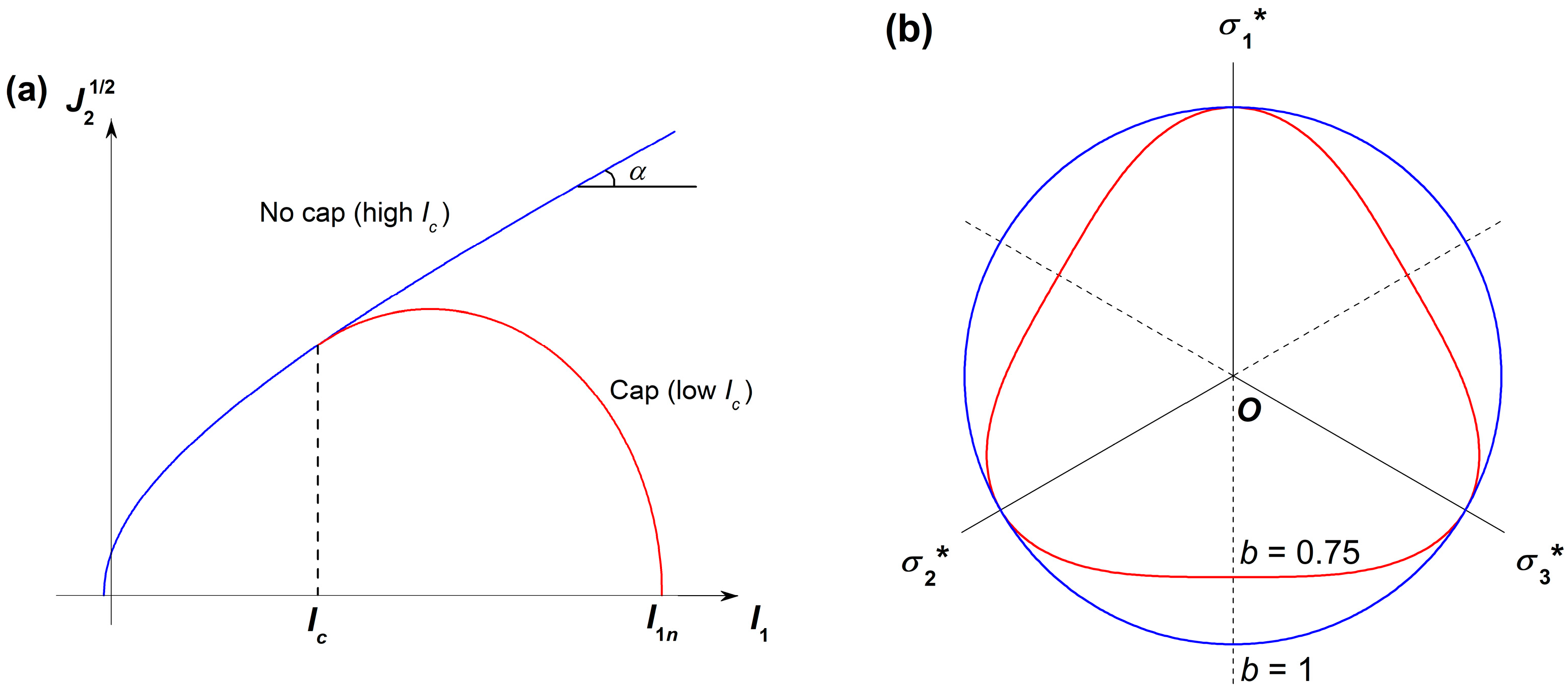
Figure 1 shows a typical representation of the MSDP_u criterion in the I₁–J₂^1/2 plane (Figure 1a) and π-plane (Figure 1b). In the I₁–J₂^1/2 plane, the MSDP_u envelope can be decomposed into two main parts. In the first part when I₁ ≤ I_c, J₂^1/2 increases nonlinearly with I₁. In the second part when I₁ > I_c, the cap controls the yield surface and J₂^1/2 tends to decrease with an increasing I₁. For dense geomaterials such as hard rocks, the values of I_c and I_1n can be very high so the cap can be neglected for most applications; this is not the case however for porous materials such as soils, backfills and some weak rocks. In the π-plane, the usual shape of the MSDP_u envelope defined above by Equation (8) depends on the value of parameter b. The typical value of b goes from 1 to about 0.7 and the corresponding envelope evolves from a circle (for b = 1) to a rounded triangle (b < 1) in the π-plane, as shown in Figure 1b.

The main characteristics of the MSDP_u criterion can be summarized as follows:

• At low mean stress, the criterion reduces to the Mises-Schleicher criterion (for b = 1). As the mean stress increases, the MSDP_u surface in the I₁–J₂^1/2 plane becomes linear with a slope angle α (Figure 1a), similarly to the DP criterion (for b =1).
• The MSDP_u surface has no sharp apex (corner) for negative I₁ values. This curved shape produces a natural tension cut-off that is physically and experimentally more representative than many other criteria. It is also advantageous from a numerical point of view because no extra algorithm operation is needed to handle the corner or apex [2,33,34,35].
• The rounded surface depends on the Lode angle θ so it can take into account the effect of the loading geometry in the π-plane (again without corners).
• The limiting pressures for the cap onset I_c and closure I_1n can be determined explicitly from experimental testing. The cap curvature can also be related to experimental data and then used to define the volumetric strain (through the plastic potential Q).
• The criterion becomes insensitive to the mean stress when α = 0 or ϕ = 0°; unconsolidated-undrained (UU) conditions can thus be simulated.
• The criterion can be applied to a wide variety of geomaterials, from low porosity rocks, to stiff soils and to high porosity materials (e.g., porous rocks, loose soils and backfill); it has also been applied to other types of engineering materials such as metals and ceramics.

Additional details can be found in Aubertin et al. [20,21], Aubertin and Li [12] and Li et al. [23].

3. Implementation of the Multiaxial MSDP_u-EPP Model in FLAC3D

The constitutive model formulation in FLAC3D can be expressed in terms of the principal stresses σ₁, σ₂, σ₃ and the principal strains ε₁, ε₂, ε₃, using procedures described by Itasca [25]. The total strain increment Δε_i can be divided into elastic Δε_i^e and plastic Δε_i^p strain increments (with i = 1, 2, 3)

$$\Delta {\epsilon }_i=\Delta {\epsilon }_i^e+\Delta {\epsilon }_i^p$$

(14)

The principal stress increments associated with the elastic strain increments can then be expressed as follows:

$$\begin{gathered} \Delta {\sigma }_1=S_1\left(\Delta {\epsilon }_1^e,\Delta {\epsilon }_2^e,\Delta {\epsilon }_3^e\right)={\beta }_1\Delta {\epsilon }_1^e+{\beta }_2\left(\Delta {\epsilon }_2^e+\Delta {\epsilon }_3^e\right) \\ \Delta {\sigma }_2=S_2\left(\Delta {\epsilon }_1^e,\Delta {\epsilon }_2^e,\Delta {\epsilon }_3^e\right)={\beta }_1\Delta {\epsilon }_2^e+{\beta }_2\left(\Delta {\epsilon }_1^e+\Delta {\epsilon }_3^e\right) \\ \Delta {\sigma }_3=S_3\left(\Delta {\epsilon }_1^e,\Delta {\epsilon }_2^e,\Delta {\epsilon }_3^e\right)={\beta }_1\Delta {\epsilon }_3^e+{\beta }_2\left(\Delta {\epsilon }_1^e+\Delta {\epsilon }_2^e\right) \end{gathered}$$

(15)

where S₁, S₂, S₃ are linear functions for the Hooke’s law; β₁ and β₂ are material parameters (constants) defined in terms of the isotropic shear modulus G and bulk modulus K,

$$\begin{gathered} {\beta }_1=K+\frac{4}{3}G \\ {\beta }_2=K-\frac{2}{3}G \end{gathered}$$

(16)

The plastic strain increment is given by the flow rule

$$\Delta {\epsilon }_i^p=\lambda \frac{\partial Q}{\partial {\sigma }_i}$$

(17)

where σ_i is the current stress state component (or initial stress state); λ is plastic coefficient; Q is the plastic potential (function), defined as follows

$$Q=J_2-\xi F_0^2{F}_{\pi }^2$$

(18)

where coefficient ξ serves to control the plastic deviatoric and volumetric strain components. When ξ = 1, the plastic potential function is the same as the yield criterion (Q = F) so the flow rule is associated. When ξ ≪ 1 (very small value), the plastic potential leads to quasi-isovolumetric plastic strains, typical of critical state [15,36].

Combining Equations (14) and (17) leads to

$$\Delta {\epsilon }_i^e=\Delta {\epsilon }_i-\lambda \frac{\partial Q}{\partial {\sigma }_i}$$

(19)

Substituting Equation (19) into Equation (15) gives

$$\Delta {\sigma }_i=S_i\left(\Delta {\epsilon }_1,\Delta {\epsilon }_2,\Delta {\epsilon }_3\right)-\lambda S_i\left(\frac{\partial Q}{\partial {\sigma }_1},\frac{\partial Q}{\partial {\sigma }_2},\frac{\partial Q}{\partial {\sigma }_3}\right)$$

(20)

Under varying stress conditions, the new stress state σ_i^N corresponding to the total strain increment Δε_i is expressed by

$${\sigma }_i^N={\sigma }_i+\Delta {\sigma }_i$$

(21)

In the user-defined model, the induced (postulated) elastic stresses σ_i^I are obtained by adding a “trial” stress increment to the current (initial) stress state σ_i. The “trial” stress increment is computed by using the incremental form of Hooke’s law and the total strain increment Δε_i. The induced elastic stresses σ_i^I can be expressed as follows:

$${\sigma }_i^I={\sigma }_i+S_i\left(\mathsf{\Delta }{\epsilon }_1,\mathsf{\Delta }{\epsilon }_2,\mathsf{\Delta }{\epsilon }_3\right)$$

(22)

Substituting Equations (20) and (22) into Equation (21) leads to

$${\sigma }_i^N={\sigma }_i^I-\lambda S_i\left(\frac{\partial Q}{\partial {\sigma }_1},\frac{\partial Q}{\partial {\sigma }_2},\frac{\partial Q}{\partial {\sigma }_3}\right)$$

(23)

Equation (23) is called the plastic correction in FLAC3D.

The induced elastic stresses are initially taken as the new stress state and then adjusted if required. When the new stress state is within the elastic domain (i.e., F < 0), the new stress state is updated by directly using the incremental expression of Hooke’s law. When the new stress state would lead to F > 0, the plastic coefficient λ is calculated from the MSDP_u yield criterion to bring the new stress state σ_i^N determined by Equation (23) on the yield surface (F = 0), which results in

$$F\left({\sigma }_1^N,{\sigma }_2^N,{\sigma }_3^N\right)=J_2^N-{\left(F_0^N\right)}^2{\left(F_{\pi }^N\right)}^2=0$$

(24)

Substituting Equation (23) into Equation (24) gives the quadratic equation:

$$A{\lambda }^2+B\lambda +C=0$$

(25)

The correct value of λ corresponds to the root with smaller absolute value of the two obtained after solving Equation (25).

Since F₀ includes two pieces and depends on the value of I₁, the expressions of A, B and C in Equation (25) depend on whether (or not) I₁ ≤ I_c. Hereafter, their expressions are introduced with “s” denoting a shear response (for I₁ ≤ I_c) and “v” denoting the contribution of a volumetric response related to the cap (I₁ > I_c).

When I₁ ≤ I_c, F₀ becomes

$$F_0^s={\left[{\alpha }^2\left(I_1^2-2a_1{I}_1\right)+a_2^2\right]}^{1/2}$$

(26)

The corresponding plastic potential is then expressed as

$$Q^s=J_2-\xi {\left(F_0^s\right)}^2{F}_{\pi }^2$$

(27)

The expressions for A^s, B^s and C^s are given in Appendix A.

When I₁ > I_c, F₀ is written as

$$F_0^v={\left[{\alpha }^2\left(I_1^2-2a_1{I}_1\right)+a_2^2-a_3{\left(I_1-I_c\right)}^2\right]}^{1/2}$$

(28)

and

$$Q^v=J_2-\xi {\left(F_0^v\right)}^2{F}_{\pi }^2$$

(29)

The expressions for A^v, B^v and C^v are given in Appendix B.

To simplify the calculations of partial derivatives, variation of Lode angle θ is postulated to have a negligible effect on F_π to obtain the new (updated) stress state (from the induced elastic stresses). This simplification leads to the following function in the π-plane:

$$F_{\pi }^N\approx F_{\pi }^I=\frac{b}{{\left[b^2+\left(1-b^2\right){\sin }^2\left(45°-1.5{\theta }^I\right)\right]}^{1/2}}$$

(30)

with

$${\theta }^N\approx {\theta }^I=\frac{1}{3}{\sin }^{-1}\frac{3\sqrt{3}{J}_3^I}{2\sqrt{{\left(J_2^I\right)}^3}}$$

(31)

The computational procedure of the MSDP_u-EPP model in FLAC3D v6.0 (Itasca, 2017) starts with adding the stress components, which are computed from the incremental Hooke’s law by using the total strain increments to the current (initial) stress state σ_i and the induced elastic stresses σ_i^I are obtained (Equation (22)). Then, the σ_i^I values are substituted into the yield function F to determine if these are in the elastic domain (F < 0) or the plastic domain (F ≥ 0). If in the elastic domain, the new (updated) stress state σ_i^N equals to σ_i^I. If in the plastic domain, the new stress state σ_i^N is updated by applying the plastic correction (Equation (23)) to σ_i^I. The “corrected” new principal stresses σ₁^N, σ₂^N and σ₃^N can then be used to update the stress tensor σ_ij in the system of reference axes, assuming that the principal directions have not been affected by the occurrence of a plastic correction.

Figure 2 shows the computational scheme for the implementation of the non-associated MSDP_u-EPP model in FLAC3D 6.0 [25]. As indicated above, FLAC3D v6.0 provides the option to load and run user-written model in DLL (dynamic link library). The implementation of the MSDP_u-EPP model was hence performed by creating a user-written DLL, which was created by compiling a program written with C++ language in Visual Studio 2017.

4. Validation of the FLAC3D MSDP_u-EPP Model

After its implementation in FLAC3D, preliminary simulations with the user-defined MSDP_u-EPP model were conducted to verify that the formulation and code programming were correctly done and to validate (in part) the numerical results. The main results from this assessment are summarized here.

The first validation is made against the analytical solution for the stresses around a cylindrical opening in a MSDP_u-EPP material developed by Li et al. [23] for the open MSDP_u surface (without cap) and the solution of Li and Aubertin [37] with the closed MSDP_u yield surface (with cap). It should be noted that the analytical solutions were developed for a constant Lode angle θ = 0°, even though the actual Lode angle tends to vary slightly in the plastic region (between about −19° and −25°) along radial coordinate r around the cylindrical opening, while θ = 0° in the elastic region [23,37].

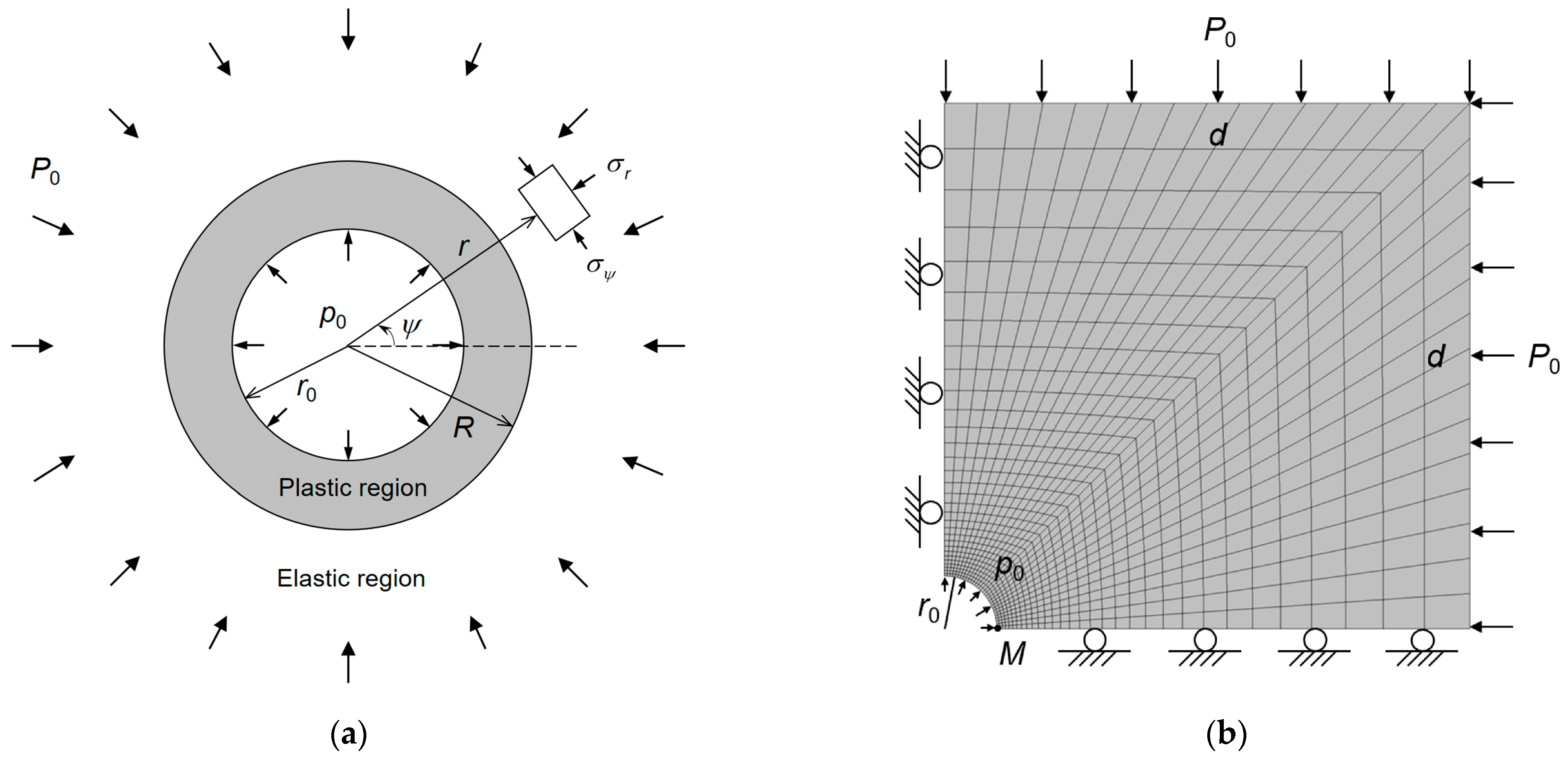
Figure 3a shows a cylindrical opening in an elastic-perfectly plastic material subjected to a hydrostatic far-field stress P₀; an internal pressure p₀ is applied to the wall of the cylindrical opening (in plane strain condition). In the figure, r₀ is the radius of the opening, R is the radius of the interface between the plastic and elastic regions, σ_r and σ_ψ are the radial and tangential stresses respectively and r and ψ are the corresponding cylindrical coordinates. The calculations are made for r₀ = 1 m, P₀ = 30 MPa and p₀ = 2 MPa. The MSDP_u-EPP model parameters are given in

Table 1. Parameters used for comparing the results obtained with the FLAC3D MSDP_u-EPP model and analytical solutions (taken from Li and Aubertin [37]).

Parameter	G (GPa)	K (GPa)	C0 (MPa)	T0 (MPa)	ϕ (°)	Ic (MPa)	a3
With cap	20	60	7	0.2	27	10	0.06
No cap	20	60	7	0.2	27	-	0

.

Figure 3b shows a numerical model with domain size d × d and the boundary conditions. The model built with FLAC3D takes advantage of the quarter-symmetry geometry. The analytical solutions were developed for a plane-strain condition, so the numerical simulations are conducted in 2D even if the MSDP_u-EPP model implemented in FLAC3D is three-dimensional. A commonly used method to do that is to isolate a thin domain in the direction perpendicular to the axis, with the displacements fixed in the direction parallel to the opening axis but allowed in the directions perpendicular to the axis. The thickness t of the modeling domain is taken as one-fifth of the cylinder radius, i.e., t = 0.2 m.

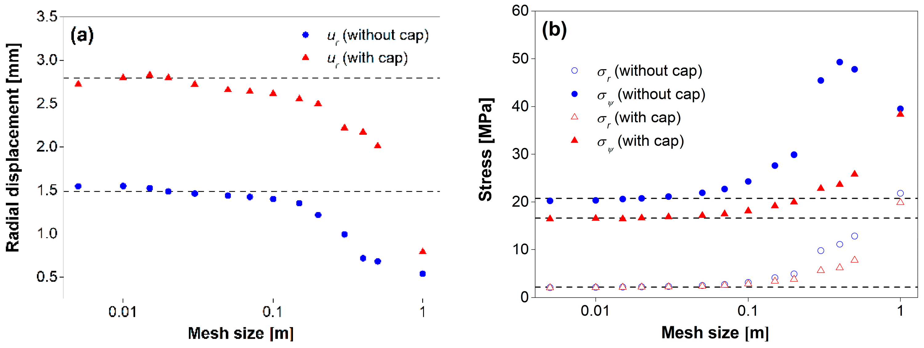
A sensitivity analysis was conducted to obtain an optimal configuration of the numerical model, which is based on an optimal domain size and optimal mesh. The optimal domain corresponds to the smallest size of the model to minimize the time of calculation and large enough to ensure stable and reliable numerical results. Similarly, an optimal mesh size m is associated with the coarsest elements (blocs) to minimize the time of calculation, with elements that are fine enough to ensure stable and reliable numerical results.

Figure 4 shows the variation of the radial displacements (Figure 4a) and stresses (Figure 4b) at a reference point M (shown in Figure 2) as a function of the mesh size (for domain size d = 10 m). In this figure, the mesh size is defined from the minimum size of the first layer of the grid around the opening, which increases at a constant ratio from the opening wall to the domain boundary (based on radial meshing; Itasca [25]). The results shown in Figure 4 indicate that, for both versions of the MSDP_u-EPP model (with and without the cap), the numerical results tend to become stable once the mesh size is equal to or smaller than 0.02 m. The optimal mesh size corresponds to m = 0.02 m.

Figure 5 shows the variation of the radial displacements (Figure 5a) and stresses (Figure 5b) as a function of the domain size (with m = 0.02 m). It can be seen that d = 10 m is the smallest value, which remains large enough to ensure stable and reliable numerical results. The optimal numerical model is then constructed with m = 0.02 m and d = 10 m, which are used to conduct the numerical simulations.

Figure 6 shows the radial (σ_r) and tangential (σ_ψ) stress distributions obtained from the numerical modeling and analytical solution for the cases of a closed MSDP_u surface (Figure 6a) and an open MSDP_u surface (Figure 6b). The agreements between the numerical and analytical results are excellent in all cases. Additional calculations were also made for other material parameters and loading conditions (results not shown here) to help assess the validity of the MSDP_u-EPP model and its numerical implementation in FLAC3D. The good agreements obtained between the numerical and analytical results support the validation and indicate that the analytical solutions developed by considering a constant Lode angle provide a good approximation of the stress distribution around a cylindrical opening.

The second component of this validation of the FLAC3D MSDP_u-EPP model is performed against the analytical solution of Salençon [38,39], developed for evaluating the distribution of stresses and radial displacements around a cylindrical opening in a MC-EPP material (considering an associated flow rule). Parameter ξ = 1 (associated flow rule) and a₃ = 0 (without cap) are thus taken for the FLAC3D MSDP_u-EPP model. As the MSDP_u is nonlinear and MC is linear in the I₁–J₂^1/2 plane, the MC strength parameters ϕ and c were chosen so the two yield surfaces would correlate to each other (as well as possible) in the stress domain of interest around the cylindrical opening (for 50 MPa ≤ I₁ ≤ 100 MPa in this case). The resulting MC strength parameters are ϕ = 32° and c = 3.9 MPa for matching the open MSDP_u surface with the parameters given in Table 1. The two yield surfaces in the I₁–J₂^1/2 plane (for θ = 0°) are very close to each other for the stress states of interest, as shown in Figure 7. A constant Lode angle θ = 0° is again considered an acceptable approximation for the stresses around the cylindrical opening.

Figure 8 illustrates the distributions of the stresses (Figure 8a) and radial displacements (Figure 8b), obtained from FLAC3D MSDP_u-EPP model and calculated with the analytical solutions of Salençon [38,39]. The good agreement between the two types of solutions indicates that the FLAC3D MSDP_u-EPP model correctly represents the problem at hand. This (partial) validation supports the use of the FLAC3D MSDP_u-EPP model to analyze the elastoplastic response of geomaterials around underground openings.

5. Applications of the FLAC3D MSDP_u-EPP Model

In order to further assess the features of the new FLAC3D MSDP_u-EPP model, simulations are conducted to analyze the mechanical response of cemented backfill in a 3D vertical mine stope.

Backfill is commonly used in underground mine excavations to ensure safe working conditions and improve ore recovery. Underground backfilling is also gaining momentum as a mine waste management approach [40]. Evaluating the stresses in backfilled stopes is of great importance and interest for underground mine stability. Until recently however, most of the numerical analyses were done under plane strain (2D) conditions. Only a few investigations have included 3D numerical analyses with the Mohr-Coulomb EPP model [27,28,29,41,42,43].

Figure 9 shows the conceptual model of a three-dimensional vertical mine stope in a semi-infinite rock mass before (Figure 9a) and after (Figure 9b) the addition of backfill. This stope is located at a depth of 500 m below the ground surface. It is excavated to a height of 45 m; the width is 6 m in the two horizontal directions (Figure 9a). After excavation, the stope is filled by a cemented (cohesive) backfill to a final height of 44.5 m, leaving a void space of 0.5 m at the top (Figure 9b). The stress distribution in the backfill and surround rock mass then depends on the fill settlement under its own weight and interaction with the rock walls. The stability of the rock walls of the empty stope is first evaluated using both MSDP_u-EPP and MC-EPP models, respectively.

Figure 10 shows the corresponding numerical model of the stope, built by FLAC3D after excavation, before backfilling. Half of the stope is modelled to take advantage of the symmetric geometry. As indicated in the figure, the boundary conditions applied to the model domain are defined with a free surface on the top boundary and a fixed surface at the base. The conditions imposed along the four external vertical surfaces allow displacements within their respective plane, but not in the perpendicular direction. The rock mass is considered homogeneous, isotropic and perfectly elastoplastic; it is characterized by the following properties: E_r = 30 GPa (Young’s modulus), ν_r = 0.3 (Poisson’s ratio), γ_r = 27 kN/m³ (unit weight). These parameters are used for both of the MC-EPP (with a tension cut-off at T₀) and MSDP_u-EPP models. The strength parameters are ϕ = 32°, c = 3.9 MPa and T₀ = 0.2 MPa for the MC criterion and ϕ = 27°, C₀ = 7 MPa, T₀ = 0.2 MPa and a₃ = 0 for the open MSDP_u criterion. The rock mass is subjected to three-dimensional in-situ stresses, including the vertical in-situ stress σ_v (z-direction) generated by the overburden (i.e., σ_v = γ_rh; h is the depth below ground surface), maximum horizontal in-situ stress in the x-direction σ_H taken as two times the vertical in-situ stress (i.e., σ_H = 2σ_z) and minimum horizontal in-situ stress in the y-direction σ_h (varying values in the different simulations).

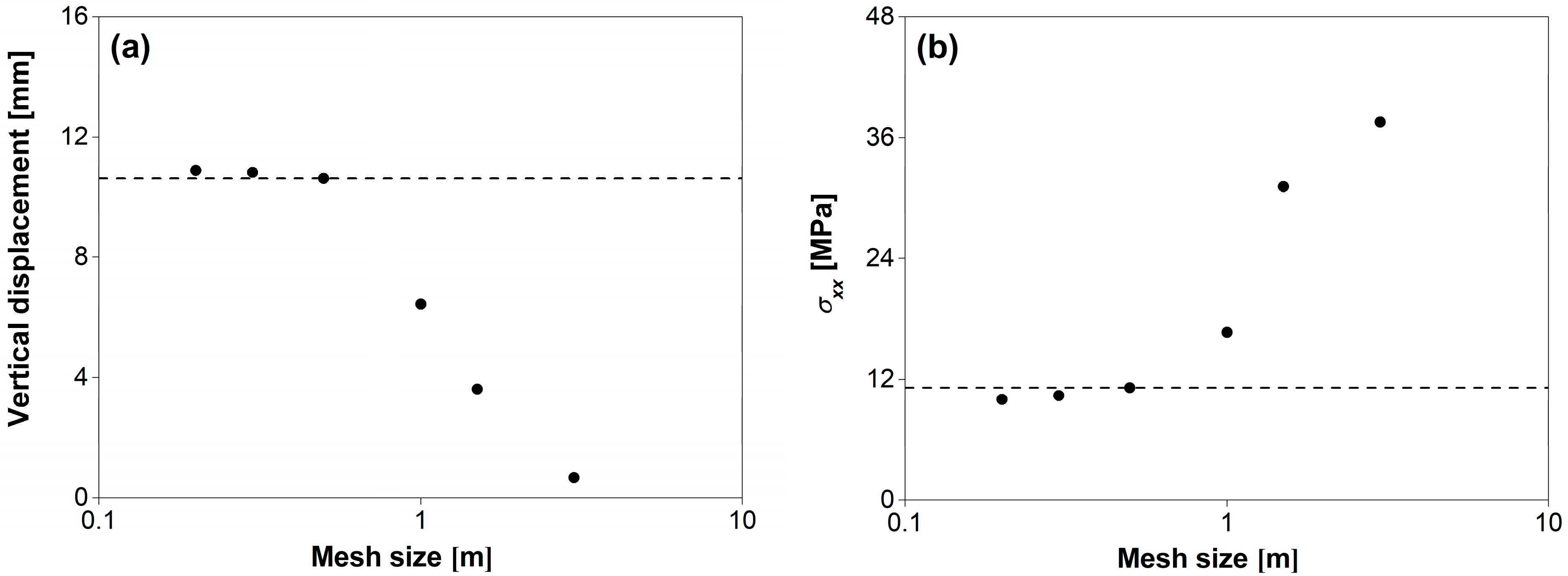
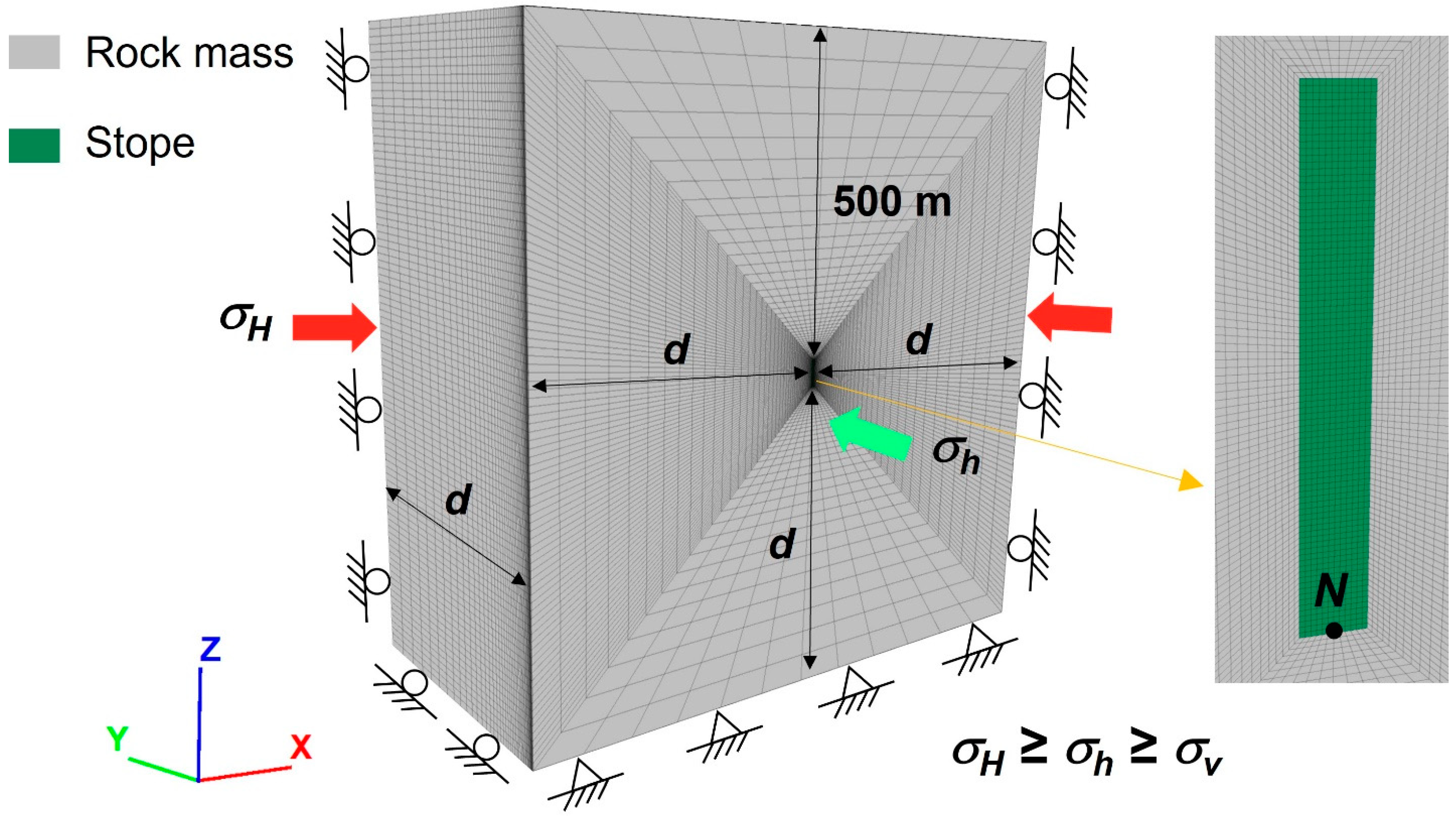
Sensitivity analyses are performed to ensure stable and reliable numerical results and obtain optimal numerical model for each case. For a numerical model such as the one shown in Figure 10, the sensitivity analysis gives the optimal mesh m and optimal domain size d.

The procedure is illustrated in Figure 11, which shows the variation of vertical displacement (z-direction) and horizontal stress σ_xx at a reference point N (at the center of the stope base, see Figs. 9a and 10) as a function of the mesh size (with d = 500 m) for simulations conducted with the MSDP_u-EPP model, for an in-situ stress state σ_h = σ_H = 2σ_z. The results indicate that stable numerical results are achieved with m = 0.5 m. 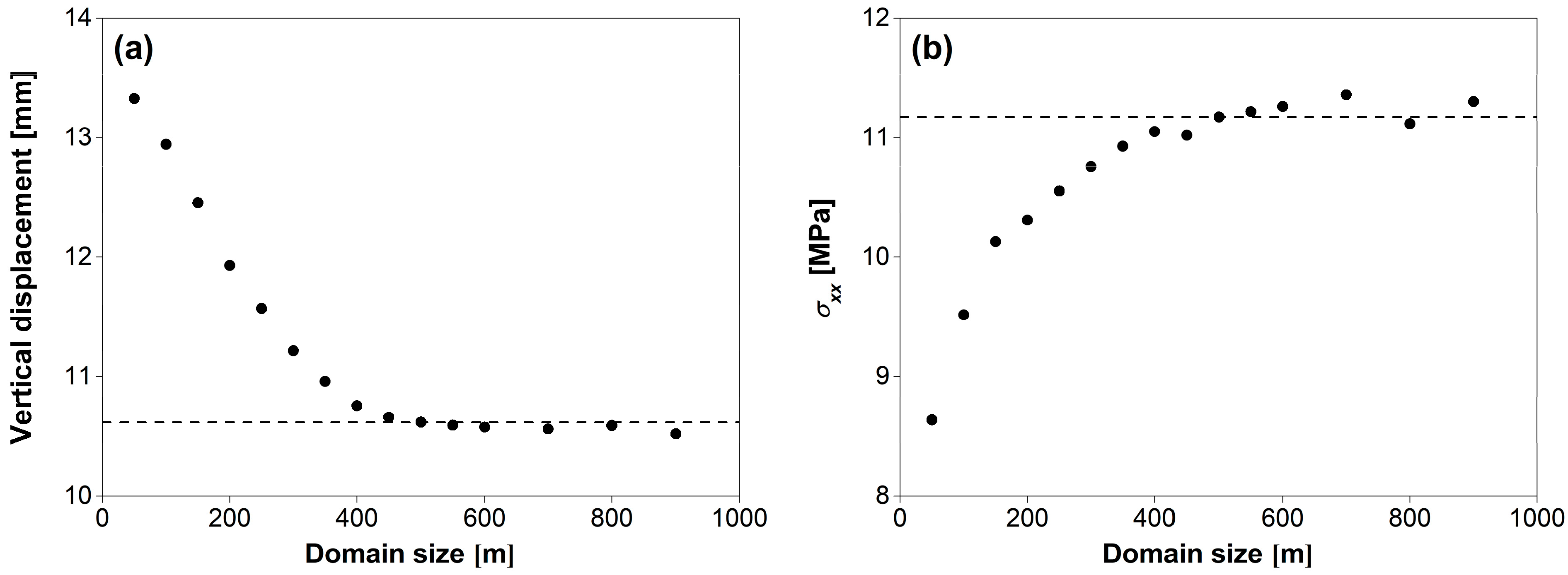Figure 12 shows the variation of the vertical displacement (z-direction) and σ_xx as a function of the domain size (with m = 0.5 m). It is seen that the numerical results become stable when the domain size d is equal to or larger than 500 m. The results thus indicate that the optimal numerical model has a mesh size of 0.5 m and a domain size of 500 m.

Figure 13 shows the yielded areas around the stope along a vertical cross cut section in the xz symmetric plane, obtained from the numerical simulations conducted with the MSDP_u-EPP and MC-EPP models, respectively. The results have been obtained for σ_h equals to 1, 1.4 and 2 times σ_v, while σ_v and σ_H are kept unchanged. It can be seen that the size of yielded area obtained with the MSDP_u-EPP model significantly increases as the intermediate in-situ stress σ_h increases from σ_v to 2σ_v, indicating that the intermediate in-situ stress plays an important role in the response and stability of openings. With the MC-EPP model however, the yielded area stays almost unchanged when σ_h increases from σ_v to 2σ_v because the MC criterion is based on the 2D formulation and thus fails to consider explicitly the effect of the intermediate principal stress in the 3D extension used in FLAC3D.

Figure 14 shows the corresponding numerical model after the placement of backfill in the stope, built with FLAC3D. As was the case for the numerical model shown in Figure 10, half of the stope is modelled to take advantage of the symmetric geometry. The boundary conditions are defined by a free top boundary surface, a fixed bottom boundary surface and four vertical external surfaces whose displacements are allowed within their respective plane, but not allowed in the direction perpendicular to that plane. The stope backfilling is performed in multiple layers after the convergence of the rock walls has been completed. The thickness of each layer is 5 m (except for the top layer having a thickness of 4.5 m). A mesh size m of 0.5 m is used for the backfill; the domain size d = 500 m, determined for the rock wall stability analysis shown in Figure 10, is also used here. As the backfill is placed in the open stope after all the elastic and plastic strains have been released, the mechanical response of the backfill is almost independent on the in-situ stresses and rock model. The rock mass is thus considered homogeneous, isotropic and linearly elastic (without yield), characterized by E_r = 30 GPa, ν_r = 0.3 and γ_r = 27 kN/m³. The vertical in-situ stress σ_v is generated by the overburden and the horizontal in-situ stress is isotropic, with σ_h = σ_H = 2σ_z.

The stresses in the backfilled stope are evaluated using the MSDP_u-EPP and MC-EPP models. The weakly cemented backfill is characterized by E_b = 300 MPa (Young’s modulus), ν_b = 0.327 (Poisson’s ratio), ρ_b = 1800 kg/m³ (density). The MSDP_u criterion is defined by ϕ = 30°, C₀ = 10 kPa, T₀ = 0.2 kPa, b = 0.75, I_c = 100 kPa and a₃ = 0.06. A value of ξ = 0.01 is used to express the plastic potential Q for the non-associated flow rule to represent the quasi-isovolumetric plastic strain of the backfill following settlement and mobilization of the frictional stress along the vertical walls. The MC yield parameters were selected so the surface would be close to the MSDP_u yield surface for comparative purposes of the stresses obtained from numerical simulations; the corresponding MC strength parameters are ϕ; = 31°, c = 3.8 kPa and T₀ = 0.2 kPa. A non-associated flow rule was imposed with ϕ_d = 0° (dilation angle). It is noted that the values of the Poisson’s ratio ν_b and internal friction angle ϕ are interrelated through ν_b = (1 − sinϕ)/(2 − sinϕ) to ensure a consistent at-rest earth pressure coefficient K₀ [28,29,44,45,46]. This results in a value of Poisson’s ratio ν_b = (1 − sinϕ) / (2 − sinϕ) = (1 − sin31°) / (2 − sin31°) = 0.327 and a Jaky’s [47] earth pressure coefficient at rest K₀ = 1 − sinϕ = 1 − sin31° = 0.485; the same value of K₀ is obtained from the equation based on Poisson’s ratio. The theoretical horizontal stress due to the overburden can then be calculated as σ_xx = K₀σ_zz.

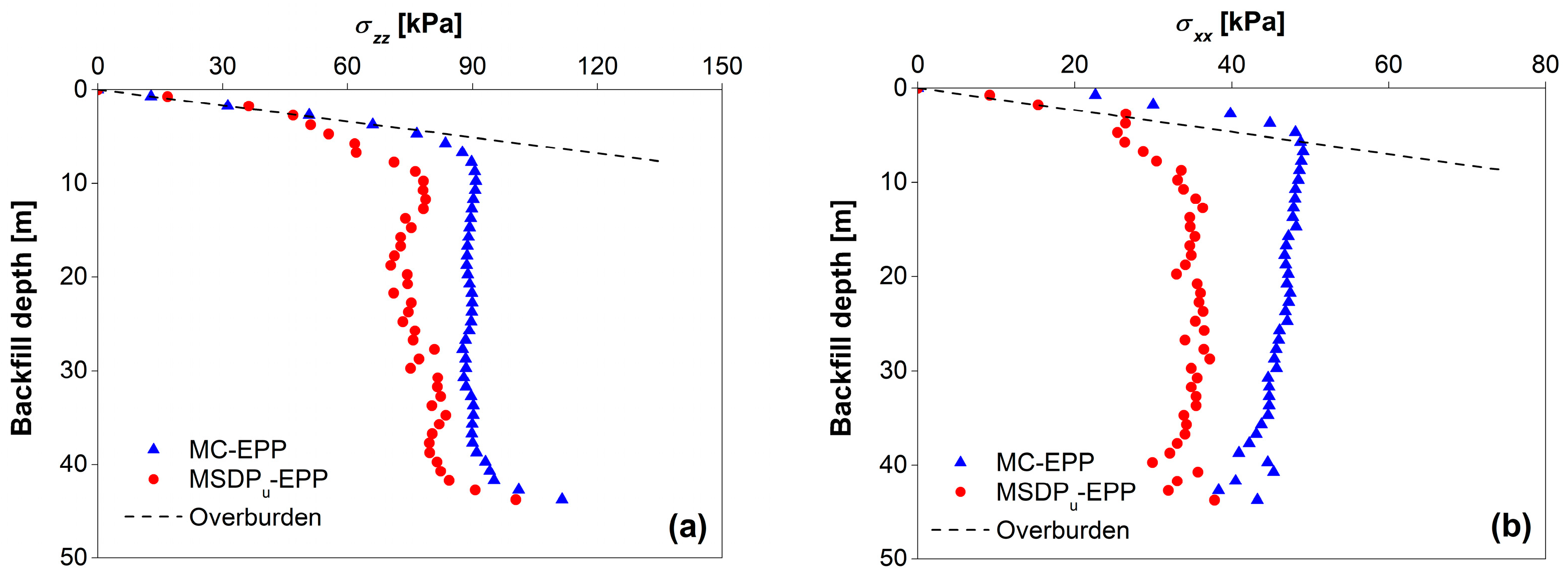
Figure 15 shows the vertical (σ_zz) and horizontal (σ_xx) stress distributions along the centerline (CL) of the backfilled stope obtained with the two models. It is seen that the general tendencies of the stress distributions obtained by numerical modeling with the MSDP_u-EPP model and MC-EPP model are similar. The vertical and horizontal stresses follow the overburden stresses (marked as dashed lines in Figure 15) at shallow depth, but the overburden stresses significantly exceed the stresses in the backfill deeper in the opening due to the well-known arching effect associated with the frictional stress transfer along the rock walls.

The trends obtained here are consistent with those given by previous numerical simulations and also by analytical solutions developed with the MC-EPP model [27,29,45,48,49]. The results shown here nonetheless indicate that the vertical and horizontal stresses obtained by the MSDP_u-EPP model are smaller than those obtained by the MC-EPP model, due to the differences in the MSDP_u and MC yield surfaces. Representative field experimental data are necessary to evaluate which one is more representative of the actual stress state.

One of the specific features of the MSDP_u-EPP model is the introduction of a cap on the yield surface, which starts at the key parameter I_c (not included in other criteria and models). As indicated above, the value of I_c controls the cap position on the yield surface, which then departs from the (quasi) linear strength increase given by the most other models. Additional simulations were conducted to investigate the effect of I_c on the stress distributions in the backfilled stope. Three values (I_c = 20 kPa, 30 kPa, 100 kPa) were used with the MSDP_u-EPP model, while the other parameters were kept constant for all cases (E_b = 300 MPa, ν_b = 0.327, ρ_b = 1800 kg/m³, ϕ = 30°, C₀ = 10 kPa, T₀ = 0.2 kPa, b = 0.75, a₃ = 0.06 and ξ = 0.01).

Figure 16 shows the vertical (σ_zz) and horizontal (σ_xx) stress distributions along the CL obtained for different I_c. The results indicate that the vertical and horizontal stresses along the CL decrease with an increasing I_c, due to the higher shear strength (larger yield surface) of the backfill. The results also indicate that the arching effect tends to become more significant for stronger cemented (cohesive) backfill. These calculations highlight the importance of including the effect of the cap through I_c, which is a unique characteristic of the MSDP_u-EPP model.

To further illustrate the features of the FLAC3D MSDP_u-EPP model with associated and non-associated flow rules, the stresses in the backfilled stope shown in Figure 9b and Figure 14 are analyzed by considering ξ = 1 for associated flow rule.

Figure 17 shows the vertical (σ_zz) and horizontal (σ_xx) stress distributions along the CL of the backfilled stope obtained by numerical modeling with the FLAC3D MSDP_u-EPP model by considering ξ = 1 (associated flow) and ξ = 0.01 (non-associated flow), respectively. It can be seen that the vertical stress along the CL is much lower for the associated flow rule than that for the non-associated flow rule (Figure 17a), due to the significant volumetric strains (dilatancy) which tend to increase the arching effect. For the same reason, the horizontal stresses along the CL for the associated flow rule significantly exceed the overburden horizontal stress at shallow depth between around 0 to 5 m (Figure 17b). Similar results have been shown by Li and Aubertin [27] with the MC-EPP model for 2D backfilled stopes. Figure 18 shows the vertical stress distribution along the CL of the 3D backfilled stope (Figure 9b and Figure 14) obtained by numerical modeling with the MC-EPP model by considering a non-associated (dilation angle ϕ_d = 0°) and associated (ϕ_d = ϕ = 31°) flow rules. The results suggest once again that the numerical modeling with an associated flow rule tends to lead an underestimation of the stresses in backfilled stopes.

6. Discussion

The non-associated MSDP_u-EPP model recently implemented in FLAC3D is applied here for the analysis of underground backfilled stopes, to illustrate some of the features of this three-dimensional nonlinear model. The MSDP_u criterion used here was previously shown to capture the essential characteristics of yielding and failure of a large variety of geomaterials, including soils, rocks and rockfills. The MSDP_u-EPP model uses a closed yield surface with a controllable cap at high mean stress. It employs a non-associated flow rule to better describe the deviatoric and volumetric plastic strains. The availability of the FLAC3D MSDP_u-EPP model will favor its application to help solve various geotechnical engineering problems such as those related to the behavior of slopes, tunnels, dams and barricades in underground mines.

Despite the various advantages of the model, there are a few limitations with the FLAC3D MSDP_u-EPP model. For instance, the model has not yet been applied to cohesionless (granular) materials such as sand, rockfill, waste rock and uncemented backfill. This can be done by expressing the MSDP_u criterion with C₀ = T₀ = 0 in Equations (10) and (11), which leads to a₁ = a₂ = 0. Equation (7) then becomes:

$$F_0={\left[{\alpha }^2{I}_1^2-a_3⟨I_1-I_c⟩{}^2\right]}^{1/2}$$

(32)

This specific version of the criterion has not yet been validated in the context of the FLAC3D MSDP_u-EPP model.

Another limitation of the model, common to all perfectly plastic models, is the absence of strain hardening and softening in the formulation. This is acceptable for many types of application, but not for some specific ones [3,4,8]. Additional work is considered for an evolving yield surface in the principal stress space with the MSDP_u-EPP model.

Also, the model has not yet been validated for coupled problems involving pore water pressures (particularly for transient conditions).

Despite such limitations, the FLAC3D MSDP_u-EPP model offers a powerful alternative to simulate the complex mechanical response of geomaterials as a built-in model in FLAC3D (and other commercial codes).

7. Conclusions

The non-associated MSDP_u elastic-perfectly plastic constitutive model (MSDP_u-EPP model) has been implemented in FLAC3D with a user-written DLL under the assistance of the C++ plug-in option. The resulting FLAC3D MSDP_u-EPP model is validated, in part, by comparing simulation results with existing analytical solutions developed for evaluating the stress and displacement distributions around cylindrical openings. The FLAC3D MSDP_u-EPP model is then used to analyze a specific three-dimensional geotechnical problem, taking into account the nonlinear stress-strain behavior, yielding and volumetric strains associated with the cap surface and considering an associated or non-associated flow rule. Application of the FLAC3D MSDP_u-EPP model is illustrated with simulations conducted to analyze the stability of a 3D open stope and stress distribution in the backfilled stope. The results were compared with those obtained with the commonly used Mohr-Coulomb (MC-EPP) model. The numerical results obtained with the MSDP_u-EPP model indicate that the size of yielded area around the empty stope significantly increases as the intermediate in-situ stress increases, indicating that the intermediate in-situ stress plays an important role in the response and stability of openings. This effect is not as clearly perceived with the MC-EPP model, however, as the simulated yielded area stays almost unchanged when the intermediate in-situ stresses are increased, hence showing that this model largely neglects this aspect. Other particular features of the FLAC3D MSDP_u-EPP model related to the closed yield envelope (with a cap) are shown with the stress analysis of backfilled stopes. These results show that when a higher mean stress is necessary to reach backfill volumetric yield surface, defined by the closed (cap) envelope, the backfill becomes stronger, leading to more pronounced arching effect and smaller stresses in the backfilled stope. This is a unique characteristic obtained with numerical simulations conducted with the FLAC3D MSDP_u-EPP model. It can thus be considered as a very useful numerical tool to analyze and solve geotechnical engineering problems. Nevertheless, improvements are still being considered for the model to minimize its limitations. For example, the model has not yet been applied to cohesionless (granular) materials; strain hardening and softening are not included in the formulation; the model has not been validated for couple problems involving pore water pressures. Work is underway to address these specific issues.