Article

Numerical Investigation on the Impact of Tailings Slurry on Catch Dams Built at the Downstream of a Breached Tailings Pond

1
School of Resources and Safety Engineering, Central South University, No.932 South Lushan Road, Changsha 410083, China
2
Research Institute on Mines and Environment, Department of Civil, Geological and Mining Engineering, École Polytechnique de Montréal, C.P. 6079 Succursale Centre-Ville, Montréal, QC H3C 3A7, Canada
*
Author to whom correspondence should be addressed.
Processes 2022, 10(5), 898; https://doi.org/10.3390/pr10050898
Submission received: 13 February 2022 / Revised: 25 April 2022 / Accepted: 29 April 2022 / Published: 2 May 2022
(This article belongs to the Special Issue Numerical Modeling in Civil and Mining Geotechnical Engineering)

Abstract

:
Tailings storage facilities (TSFs) are known as a time-bomb. The numerous failures of TSFs and the heavy catastrophic consequences associated with each failure of TSFs indicate that preventing measures are necessary for existing TSFs. One of the preventing measures is to construct catch dams along the downstream near TSFs. The design of catch dams requires a good understanding of the dynamic interaction between the tailings slurry flow and the catch dams. There are, however, very few studies on this aspect. In this study, a numerical code, named LS-DYNA, that is based on a combination of smoothed particle hydrodynamics and a finite element method, was used. The numerical modeling shows that the tailings slurry flow can generally be divided into four stages. In terms of stability analysis, a catch dam should be built either very close to or very far from the TSF. When the catch dam with an upstream slope of a very small inclination angle is too close to the tailings pond, it can be necessary to build a very high catch dam or a secondary catch dam. As the impacting force can increase and decrease with the fluctuations back-and-forth of the tailings slurry flow, the ideal inclination angle of the upstream slope of the catch dam is between 30° and 37.5°, while the construction of a catch dam with a vertical upstream slope should be avoided. However, a catch dam with steeper upstream slopes seems to be more efficient in intercepting tailings flow and allowing the people downstream to have more time for evacuation. All these aspects need to be considered to optimize the design of catch dams.

1. Introduction

Mines produce large volumes of mine waste each year in terms of tailings and waste rocks [1]. A small portion of these materials can be sent back to underground voids as backfill [2,3,4,5,6,7,8,9,10,11,12,13,14,15,16,17,18]. The recycling and reuse of these materials for in- and out-mine sites are also increasingly seen [19]. All these practices can reduce the amount of mine waste to be disposed of on the ground surface. However, due to the swelling of rocks by blasting and grinding, the large amount of tailings has to be sent by pipes to a place on the ground surface contained by dams, called a tailings storage facility (TSF), which then becomes a new perpetuity infrastructure in the environment [20,21,22,23,24,25].
Tailings are a byproduct of mill processing, containing a large portion of fine particles smaller than 80 μm and water [26]. Upon disposition in a TSF, tailings remain saturated for a long time. This is particularly true in the regions where the water balance is positive. When a TSF fails, a large volume of tailings can be instantaneously released. Their flow usually transforms into a mud flood, causing significant damage to the environment and infrastructures, and even loss of lives [27]. In 1965 in Chile, the town of El Cobre was destroyed and more than 200 people were killed due to the failure of an upstream TSF [28]. Since then, a lot of work has been done on the analysis of failure mechanisms of TSFs [29,30,31,32,33]. Despite considerable progress in the studies, failures of TSF continue to take place worldwide. In February 1994, in South Africa, the village of Merriespruit was destroyed and 17 people were killed due to the failure of an upstream TSF. On that occasion, the TSF was, for the first time, qualified by a judge as a time-bomb [34]. In China, the failure of a tailings dam at Shiqiaozi, Haicheng, Liaoning Province, on 25 November 2007 resulted in 10 people being killed, 3 reported missing, and 17 injured. Another case of a TSF failure at Taoshi, Linfen City, Xiangfen County, Shanxi Province, on 8 September 2008 involved 277 people being killed and 33 injured [28]. In 2014, in Canada, the failure of a TSF of the Mount Polley mine resulted in the release of 23.6 million cubic meters of tailings into the environment [35,36]. In November 2015, at the Samarco mine in Brazil, the failure of a TSF resulted in the death of 17 people and a flow of tailings sludge of about 800 km up to the Atlantic coast [28,37,38]. In January 2019, near Brumadinho in Brazil, 248 people were killed and 22 were reported missing due to the failure of a TSF [28,39]. These endless failures of TSFs worldwide indicate that big efforts are still needed to prevent more casualties issued from TSF failures.
The instability of a TSF can be related to a number of influencing factors, varying from technical and engineering to maintenance and management [27,29,30,34,38,39,40,41]. The technical and engineering aspects affecting the stability of TSFs include the design and construction of TSFs and their foundations. At current stage, it is impossible to entirely eliminate any risk of TSF failure [33,42]. Rather, the probability of TSF failures can even increase with time due to the persistence of existing TSFs, the ceaseless increase of the number of mines and TSFs, and the more and more pronounced climate changes, which usually have a negative impact on the stability of TSFs. Efforts should be continuously made to improve the stability of TSFs [43], install monitoring systems [44], and even forecast the scale of destructions associated with the failure of a TSF [45].
Currently, thickened or filtered tailings are widely considered as the solution of solving the physical instability of TSFs. It is, however, problematic with chemically reactive mine waste because the unsaturated tailings favor the oxidation and generation of acid mine drainage [46,47,48]. In addition, unsaturated tailings can also be prone to liquefaction, as long as the degree of saturation approaches full saturation [49], and this is probably the case in the regions where the water balance is positive. Considering this as a sure and certain solution to avoid a TSF failure could be irresponsible [21]. Moreover, work is needed to secure existing conventional TSFs. In all cases, risk analysis on the breach of TSFs is necessary [50,51,52,53,54,55,56,57,58,59,60,61,62,63,64,65]. In many cases, preventing measures can be necessary to avoid catastrophic consequences in case of a TSF failure. One of the preventing measures is to build catch dams near the downstream of a TSF. Upon failure of the TSF, the catch dams must remain stable to hold at least part of the released tailings slurry, delaying and reducing the flood of tailings. If the catch dam is not properly designed and constructed, it can fail upon the dynamic impact of a tailings slurry flood. This was the case after the breach of a TSF in March 2020 in Yichun, Heilongjiang, China. Ten catch dams had to be built, one after another, along the downstream to stop the tailings flood [66].
The purpose of this study is to obtain a good understanding of the characteristics of the tailings slurry flow after a breach of a TSF, and on the dynamic interaction between the flooding tailings and catch dams. This can ultimately help to obtain a safe and economic design of catch dams to avoid catastrophic consequences after the failure of a TSF.
Over the years, a number of works have been published on the dynamic interaction between water and downstream obstacles [67,68,69,70,71,72]. One sees also some publications on the dynamic interaction between debris flow and check dams [73,74,75,76], or even between granular material flows and obstacles [77]. These works provide a useful insight into the dynamic interaction of water, debris, and granular material with obstacles. However, very few works have been made on the dynamic interaction between tailings slurry and downstream obstacles.
Wang et al. [78] conducted numerical modeling for a specific project to study the flow characteristics of tailings upon the failure of a tailings dam. The effects of downstream dams were briefly presented without any detailed quantitative studies. Zeng et al. [79] evaluated the effect of check dam height against the debris flow of tailings slurry. A similar work has been published by Wang et al. [80], who analyzed the risk associated with the possible failure of tailings dams and the effect of a preventing dam height, built 110 m downstream from the tailings pond. All these works provide some insights on the effects of check dams on the flow of the tailings slurry. However, they were mostly for some specific projects with site-specific conditions. Much more work is needed to obtain a better understanding of the effect of downstream catch dams on the flow of a tailings slurry.
In this study, the dynamic interaction between a tailings slurry flow and a downstream infrastructure is investigated through numerical modeling, using a hybrid numerical approach with the smoothed particle hydrodynamics-finite element method (SPH-FEM). The kinetic energy of the tailings flow and the striking forces on the downstream infrastructure are evaluated. The influences of the position and upstream slope angle of the catch dam on the impact of the catch dam are, for the first time, studied. The results provide some guidelines on the layout and design of catch dams.

2. Numerical Code

Studying the characteristics of tailings slurry flow needs a numerical code that can simulate the large deformation and displacement with the time of fluid-like materials, while the fluid–structure interaction behavior can be evaluated by the conventional finite-element or finite difference method.
In this study, a numerical code, called LS-DYNA [81], based on a combination of smoothed particle hydrodynamics (SPH) and the finite element method (FEM) was used. SPH is a meshless particle method based on the Lagrangian formulation for fluid dynamics’ simulation. It was originally developed by Lucy [82], Gingold, and Monaghan [83] for three-dimensional astrophysical analysis. It is based on the hypothesis that the problem domain can be divided into a set of discrete elements, which possess or can be attributed to a certain material property. With the SPH method, large deformations can be handled without element distortions. It can thus be used to simulate dynamic problems involving large deformations, such as fluid problems with a free surface [84].
The application of the SPH method involves two approximations to represent the simulated space: the kernel and particle [85]. Figure 1 schematically shows a presentation of the SPH kernel function, W. On the figure, r is the distance between the two particles; λh denotes the influence area of the kernel function; λ is determined by the kernel function and space dimensions to satisfy the normalization condition.
In the approximation of the kernel, the spatial distance between the particles is covered by a smoothing length, over which the properties are smoothed by a smoothing kernel function. In particle approximation, the state of a system is represented by a set of particles, which possess individual material properties and move according to the conservation equations. A given particle, i, with its given velocity, density, mass, and pressure, interacts with particle j within the smoothing length. Considering the conservations of mass, momentum, and energy leads to the following expressions [87]:
d ρ i d t = j = 1 N m j v i j β W i j x i β
d v i α d t = j = 1 N m j ( σ i α β ρ i 2 + σ j α β ρ j 2 + i j ) W i j x i β
d e i d t = 1 2 j = 1 N m j ( σ i α β ρ i 2 + σ j α β ρ j 2 + i j ) v i j α W i j x i β
where ρi and ρj denote the densities of particles i and j; N denotes the number of particles; α and β denote the space vectors; x i β denotes the coordinate component of x along β; Wij denotes the smoothing function between particles i and j; v i j α and v i j β represent the velocities of particle i relative to particle j along α and β; mj denotes the mass of particle j; v i α and v j α denote the velocity components of particles i and j along α; σ i α β and σ j α β denote the total stress tensors of particles i and j; i j denotes the artificial viscosity; ei represents the internal energy of the particle i; and t represents the time.
While the SPH method is advantageous in dealing with fluids and large deformation problems, this dynamic meshless technique is much less efficient in dealing with static and small deformation problems of solid bodies than FEM [2,88]. The combination of SPH and FEM methods is thus a natural choice to deal with the dynamic interaction between fluid and infrastructures. This explains the wide application of the SPH and FEM hybrid algorithm in the simulation of the fluid–solid interaction [89].
Figure 2 shows a possible interaction between fluid particles and structure elements. The interaction between fluid and a structure is achieved by a penalty-type ‘node-to-surface’ contact algorithm. The FEM elements and SPH particles are considered as master and slave parts, respectively. The reaction force between a SPH particle and the contact surface of the structure is then proportional to the depth of the slave part on the surface of the master part. The forces exerted by the SPH particles on the FEM part are then calculated by summing up the forces exerted by each SPH particle on the FEM part.
In this study, the explicit dynamic solver of LS-DYNA® version R10.0 was employed to perform the numerical modeling based on SPH theories [91]. The applicability (usually called “validation”) of the numerical code SPH was tested against the experimental results of a slump test (see details given in Appendix A). The results indicate that the numerical code is capable of simulating the dynamic interaction between a tailings slurry and a structure.

3. Numerical Simulations of Dynamic Interaction between Tailings Flow and A Catch Dam

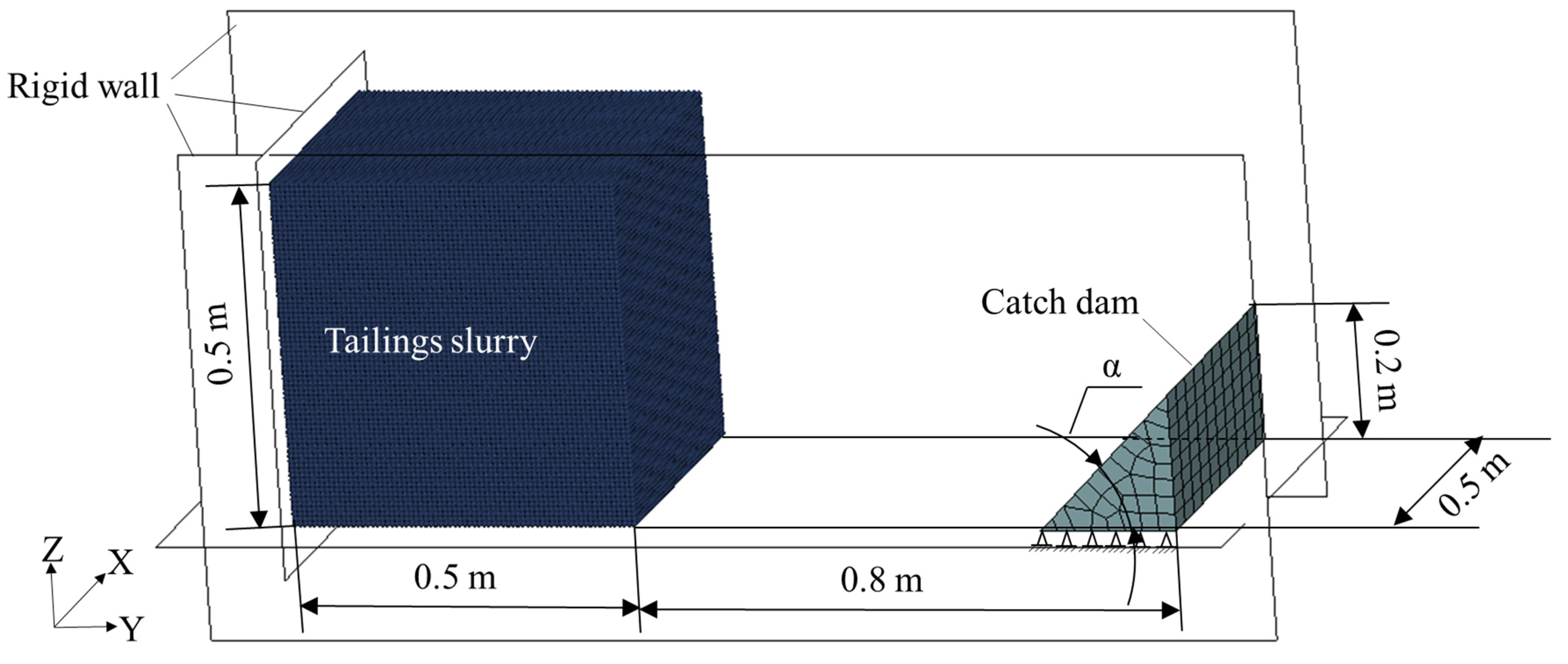
3.1. Numerical Models

Figure 3 shows a numerical model to simulate a largely reduced scale tailings pond. The tailings pond is 0.5 m long, 0.5 m wide, and 0.5 m high. The tailings slurry is the same as that used to test the applicability of the numerical code, presented in Appendix A. It is characterized by a density of 1826.6 kg/m3 and a dynamic viscosity of 0.43 Pa·s to simulate the tailings slurry having a solids content by mass of 70% of Gao [92]. The catch dam is simulated by a rigid triangular prism 0.2 m high and 0.5 m wide with an upstream slope angle α varying from 0° to 90°. The distance between the tailings pond and the catch dam is 0.8 m. The movement of the tailings particles is allowed in all directions, but only inside the open box defined by the back wall of the tailings pond, a horizontal floor and two vertical longitudinal walls. The floor and the three walls are rigid and their movements are not allowed in any direction. The tailings slurry is simulated by particles with SPH, while the rigid catch dam is built with FEM shell elements.
In this study, the flow behavior of the tailings slurry and the impact of the tailings slurry on the catch dam are analyzed by a contact algorithm with the tailings slurry and the catch dam defined as slave and master parts, respectively. The gravitational acceleration is applied along the vertical downward direction. The three vertical walls and the horizontal floor are fixed along their outside surfaces. The catch dam is fixed along its bottom. The simulations were done by considering a duration of 2.5 s, starting from the breach of the tailings pond.
For each numerical model, sensitivity analyses were made to make sure that the distinct elements were dense enough for the tailings and voids simulated by SPH (see Appendix B). These analyses showed that the tailings can be modeled with 357,911 SPH particles and a particle-to-particle spacing of 7 mm.

3.2. Numerical Results

Before the breach of the tailings pond, the tailings slurry had the highest gravitational potential energy. After the breach of the tailings pond, the tailings slurry flowed. The gravitational potential energy and kinetic energy are interconverted. It is noted that the kinetic energy K and gravitational potential energy P designate the total kinetic energy and total gravitational potential energy of the whole tailings slurry. At a given time, they can be obtained as follows:
K = i = 1 i = N m i v i 2 2
P = i = 1 i = N ( m i g h i )
where mi, vi, and hi are the mass, velocity, and elevation of SPH particle i, respectively; N is the total number of SPH particles of the tailings slurry; and g is the gravitational acceleration.
Figure 4 shows the flow states of the tailings particles at different times (T) starting from the breach of the tailings dam, with the catch dam having an upstream slope angle of α = 30°. At T = 0 s, when the tailings dam instantaneously collapses, the potential energy of tailings slurry is the highest and ready to be released. No particle moves and the kinetic energy is zero (Figure 4a). At T = 0.24 s, the upper front part of the tailings falls, moves forward and reaches the catch dam with a maximum velocity of 4.40 m/s (Figure 4b). At T = 0.5 s, all the upper part of the tailings starts moving. The front line of the tailings flood rushes away from the catch dam at a velocity of 3.31 m/s. Due to this high velocity and the slope inclination of the catch dam’s upstream, the movement of the front line is upward, almost parallel to the surface of the upstream slope (Figure 4c). At T = 0.76 s, more tailings at the top start to move and the front line of the tailings flood continues rushing away from the catch dam, but falling toward the floor. The maximum velocity of the front line is 3.92 m/s (Figure 4d). At T = 1.2 s, all the particles of tailings that can move have moved. It is interesting to note that the tailings slurry near the upstream of the catch dam is not only higher than the catch dam, but also higher than the remnants of the tailings pond. This is probably due to the drag effects by the friction of the upper mobile particles and the suction of front particles. In addition, it should be noted that a back flow of the tailings slurry takes place at the toe of the catch dam’s downstream (Figure 4e). This back flow may have a negative impact on the stability of the catch dam. At T = 2.5 s, the crest of the tailings flood moves back toward the tailings pond (Figure 4f). This phenomenon is well-known as sloshing [93,94]. Finally, one notes that the tailings particles near the rigid back walls of the tailings pond always show delayed movement, probably due to the friction and viscosity along the tailings–wall interfaces (see Figure 4b,c,f).
Figure 5 shows the variation of the tailings’ kinetic energy (Figure 5a) and impacting force (Figure 5b) exerted by the tailings flood on the catch dam’s upstream slope surface as a function of time since the breach onset of the tailings dam. One sees that the flow characteristics of the tailings slurry can generally be divided into four stages:
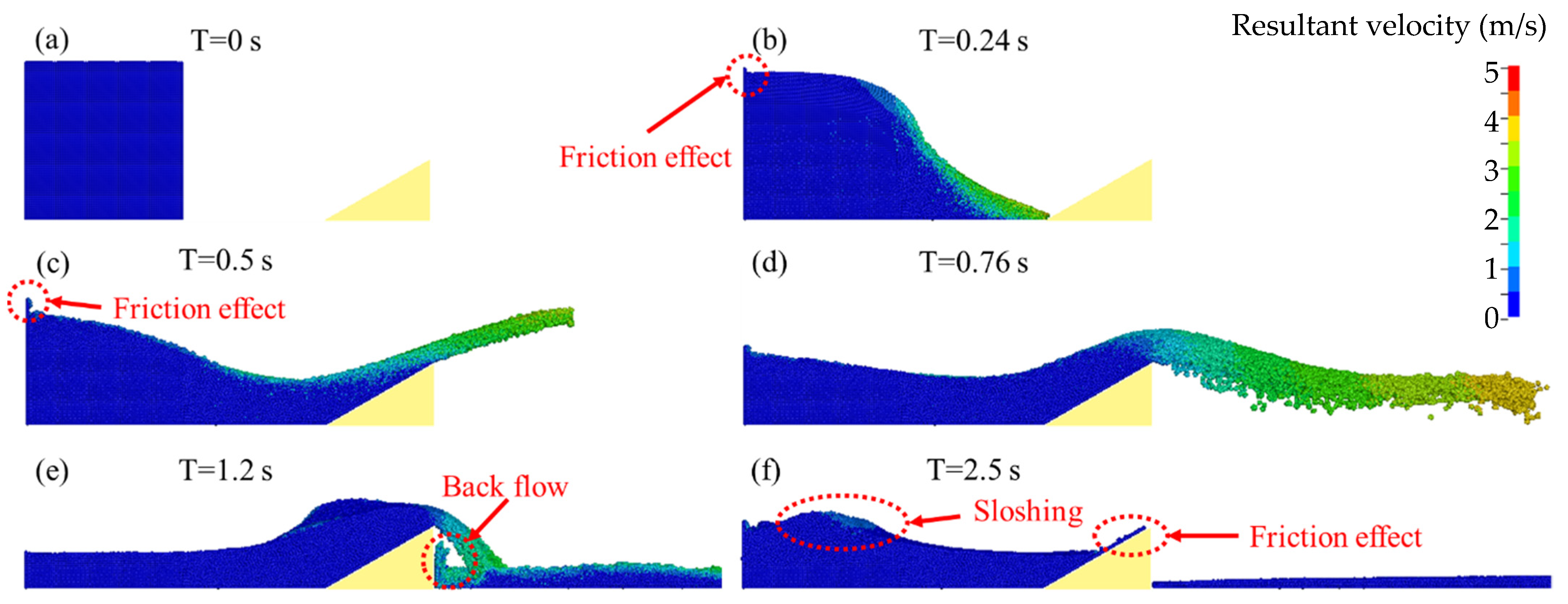
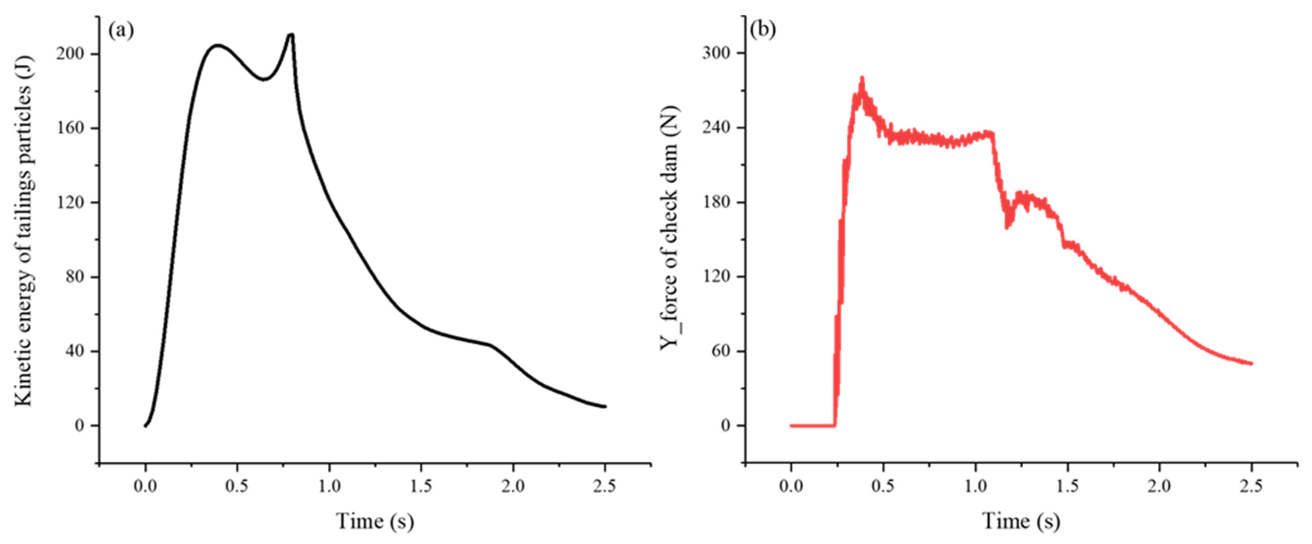
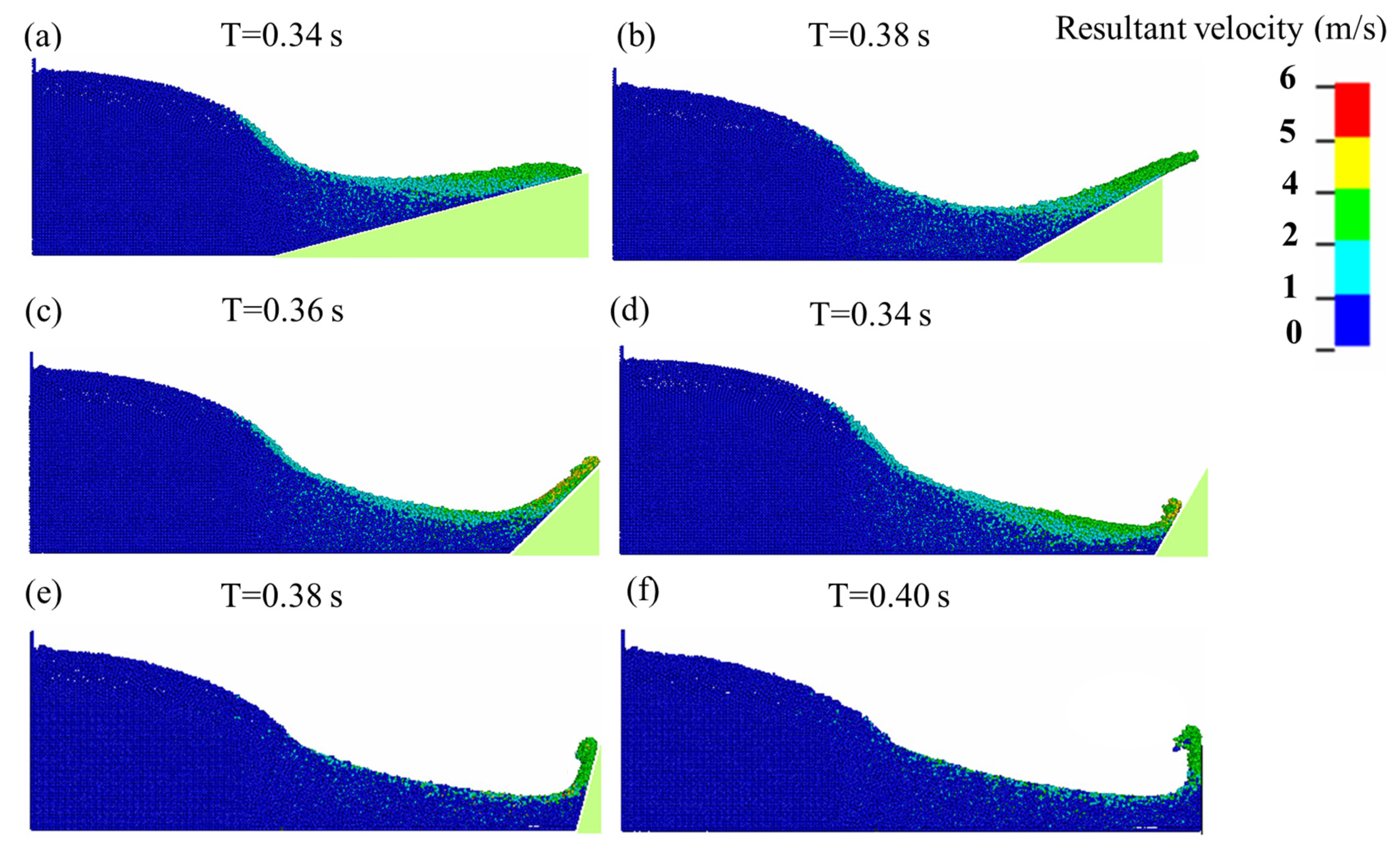
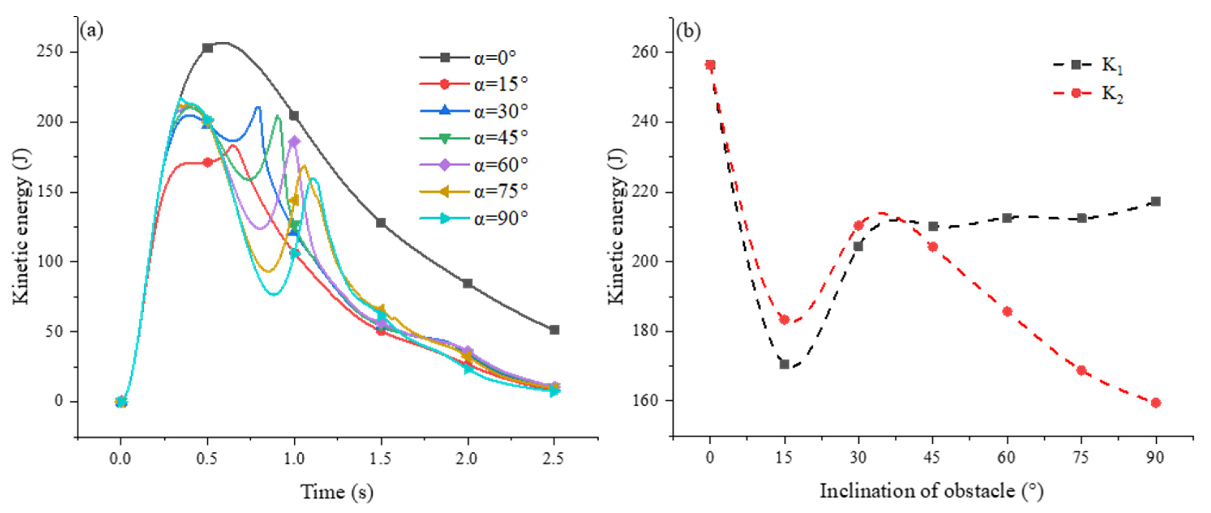
  • Stage 1: Initiation. This stage starts at the breach onset of the tailings dam at T = 0 s and ends at T = 0.38 s when the kinetic energy and impacting forces reach their first peak values. Upon the breach of the tailings dam at T = 0 s, the front part of the tailings tends to flow, driven by the potential energy. Once started, the movement of the tailings particles accelerates upon their residual potential energy and the pushing forces exercised by the upper and back particles. Subsequently, the kinetic energy continuously increases with time. At T = 0.24 s, the front line of the tailings flood reaches the toe of the catch dam. The upstream slope of the catch dam starts to receive an impacting force. After then, the tailings slurry flows upward over the upstream slope of the catch dam. A part of the kinetic energy has to be transferred into the potential energy required to allow the rising of the tailings particles. This leads to a decreased pace in the increase of kinetic energy until a peak value at T = 0.38 s when the impacting force also reaches its first peak value.
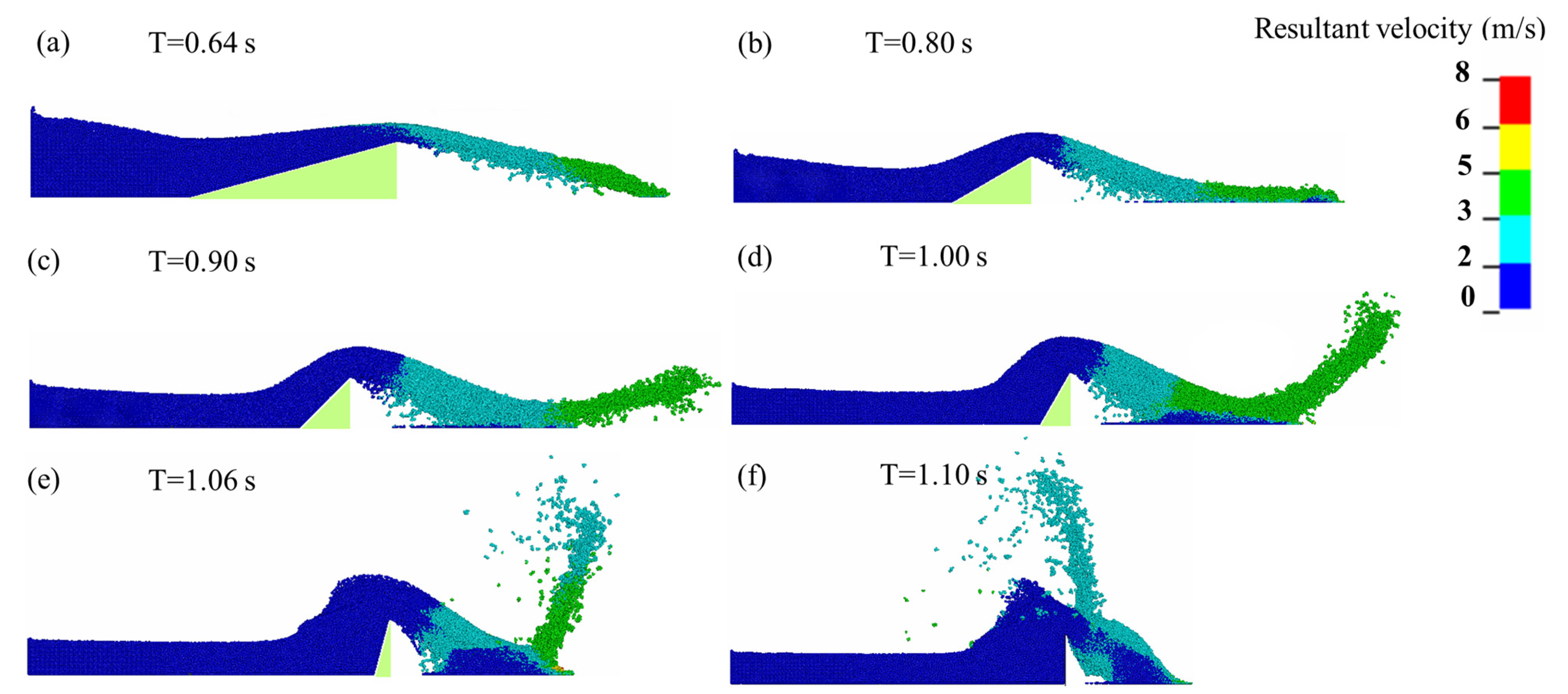
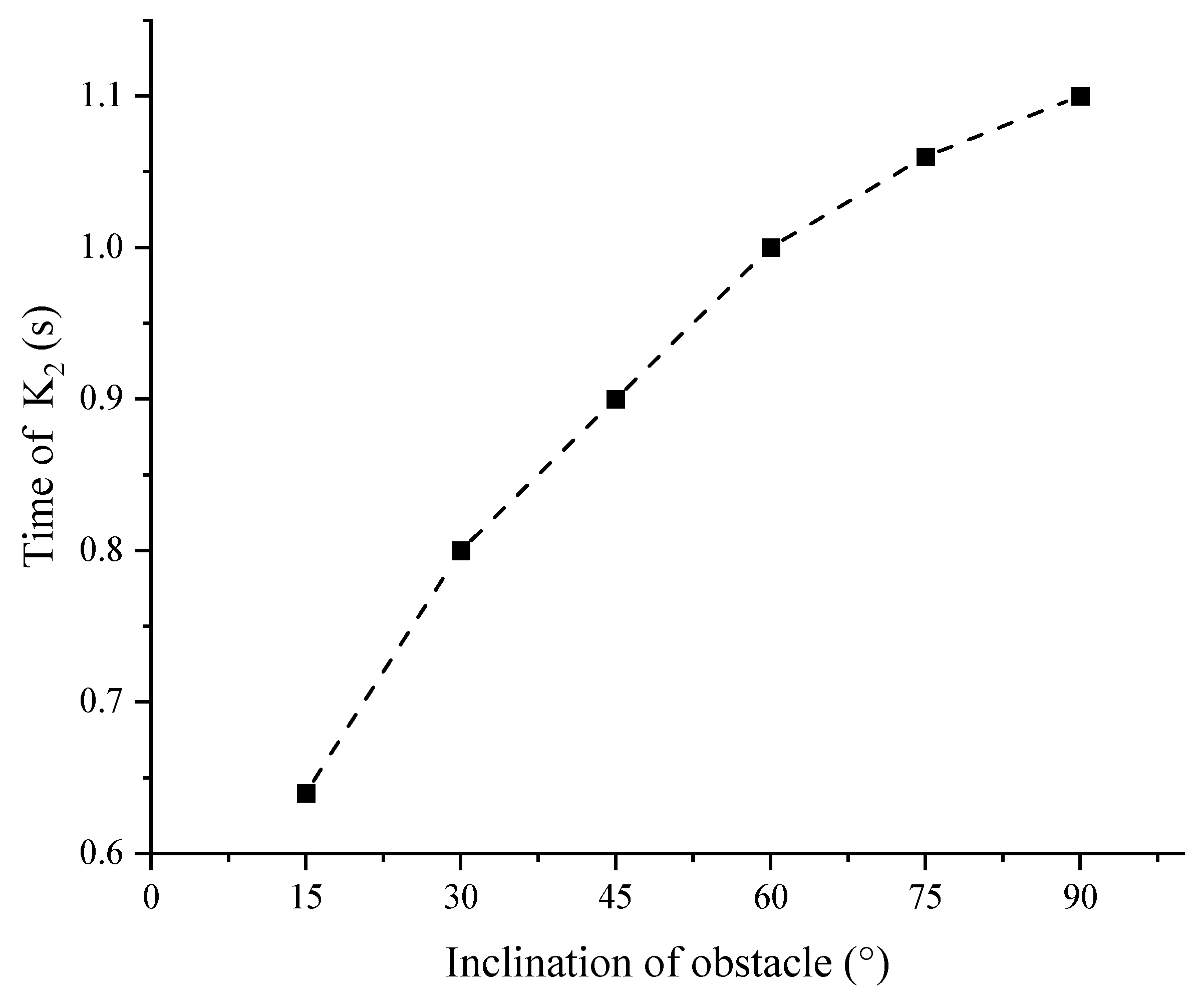
  • Stage 2: Peak stage. This stage starts at T = 0.38 s when the kinetic energy and impacting forces reach their first peak values, and ends at T = 0.76 s when the front line of the tailings flow touches the floor. In this stage, the kinetic energy and impacting force first exhibit a decrease from their peak values and then an increase until a second peak value. At T = 0.50 s, the front of the tailings flow rises to the maximum height of 37 cm. At T = 0.76 s, the front line of the tailings flow touches the floor and the kinetic energy starts to decrease. Despite their changes with time, the magnitudes of kinetic energy and impacting force remain at relatively high levels.
  • Stage 3: Ebb. This stage starts at T = 0.76 s when the kinetic energy starts to decrease, and ends at T = 1.2 s when the crest of the tailings flood starts to retreat back toward the tailings pond. During this stage, the kinetic energy continuously decreases while the impacting force keeps almost constant.
  • Stage 4: Sloshing. This stage starts from T = 1.2 s when the crest of the tailings flood starts to retreat toward the tailings pond. In this stage, the crest of the tailings slurry can first move back toward the tailings pond, and after, it can then move forward toward the catch dam. This back-and-forth can take several rounds until an equilibrium is reached. Despite these back-and-forth movements, the kinetic energy and impacting forces decrease with time.
Additional simulations have been done to analyze the effects of the upstream slope inclination angle of the catch dam on the kinetic energy and impacting forces. Figure 6 shows the flow states of the tailings particles when the catch dam’s upstream slope starts to be more or less fully covered by the tailings slurry, with the inclination angle α varying from 15° to 90°. Firstly, one sees that the tailings flow rises smoothly along the slope when the catch dam’s upstream slope has a small inclination angle. Backflow of the tailings front and splashing are observed when the slope inclination becomes abrupt. Secondly, as the distance between the front toe of the tailings and the catch dam’s downstream slope toe is kept constant at 0.8 m (see Figure 3), the distance between the front toe of the tailings and the catch dam’s upstream slope toe decreases as the inclination angle α decreases. The tailings flow thus meets the catch dam and covers the upstream slope earlier with a smaller inclination angle α. The catch dam can play its role of resistance earlier, largely reducing the maximum value of velocity. From this point of view, it seems that the catch dam should be constructed as close as possible to the tailings dam. However, when the catch dam with an upstream slope of a very small inclination angle is very close to the tailings pond, a greater quantity of tailings slurry may flow out over the catch dam. Another catch dam along the downstream of the catch dam may be necessary. These results indicate that an optimization process is necessary by considering the position, height, and upstream slope inclination angle of the catch dam, as well as the volume of tailings slurry to be confined.
Figure 7a shows the impacting forces as a function of time for different values of α, while Figure 7b presents the peak and trough values of the impacting forces as a function of the upstream slope inclination angle α of the catch dam. One sees that the trends of impacting force evolution for different inclination angle values are quite similar (Figure 7a). For a given inclination angle α, the impacting force increases to a peak value rapidly after the tailings flow reaches the catch dam. After then, the impacting force decreases to a minimum value. After a short stage of fluctuations accompanied with slight increases, the impacting force dramatically decreases to a trough value (almost −400 N for the case of α = 90°) and sharply increases to almost the same level before falling. After then, another wave of fluctuations can be observed, but the impacting force generally decreases toward zero. It is interesting to note that these results have a certain similarity with those obtained by the numerical modeling performed by Calvetti et al. [95] on the interaction between the flow of dry granular material and rigid barriers. In the latter case, the impacting force also increases with time until a peak value. After then, the impacting force decreases almost monotonously with time, showing neither a second peak, nor a negative value. This last behavior is a particularity belonging to the flow of tailings slurry associated with the sloshing and possible suction.
By comparing the flow state of tailings and the impacting force evolution, one notes that the impacting forces reach their maximum peak value when the catch dam’s upstream slope is almost fully covered by the tailings flow, while the minimum trough value corresponds to the moment of backflow, which tends to pull the upstream slope by suction toward the tailings pond. These results are important for the stability analyses of catch dams. On the one hand, the impacting force should be kept as small as possible in order to avoid pushing the catch dam away, but on the other hand, negative values should be avoided because the upstream slope of the catch dam can be disintegrated by the pulling forces if the catch dam is built with an uncemented or lowly cemented, cohesionless material. The difference between the peak and trough values should also be minimized in order to prevent a cycle loading on the catch dam’s upstream slope. From Figure 7b, one sees that the smallest peak value of the impacting force and the smallest difference between the peak and trough values of the impacting force are obtained when the inclination angle α is 30°. The largest peak value of the impacting force and the largest difference are observed when the inclination angle α is 90°. These results tend to indicate that the optimum inclination angle α is 30°, while the construction of the catch dam with a vertical upstream slope represents the highest risk and should be avoided in terms of stability for the catch dam.
Figure 8a shows the evolution of kinetic energy for different upstream slope inclination angles α. When the catch dam is absent (i.e., α = 0°), the kinetic energy of the tailings flow increases continuously and reaches a peak value of 256.5 J at T = 0.58 s, followed by a gradual decrease due to the frictional resistances along the side walls and floor. These results are very important because they indicate that a catch dam should be built either very close to or very far from the tailings pond. The worst design is to construct the catch dam at a position where the kinetic energy reaches the maximum value and a very strong catch dam is necessary.
From Figure 8a, one sees that two peak values in the kinetic energy can generally be observed when a catch dam is constructed at the downstream of the tailings pond. They can be designated as K1 for the first one and K2 for the second one. The first peak value K1 for the inclination angle α = 15° is smaller and arrives earlier than the other cases, probably due to the shorter distance between the tailings downstream slope toe and the catch dam’s upstream slope toe compared to the other cases. When the inclination angle α is larger than 45°, the magnitude and arrival time of the first peak value K1 become insensitive to further variation in the inclination angle α. However, the second peak value K2 arrives later and becomes smaller as the inclination angle α increases from 45° to 90°.
Figure 8b shows the variation of the two peak values (K1 and K2) as a function of the inclination angle α. When α = 15°, both K1 and K2 are small with a relatively large difference between them. At α = 90°, the value of K1 becomes the largest while the value of K2 becomes the smallest (except in the case without a catch dam). This case should be avoided in terms of the stability of the catch dam; this is consistent with the previous analysis of the impacting force. At an inclination angle of α = 37.5°, the magnitudes of K1 and K2 become almost the same even though their values are relatively high. This result is consistent again with the previous analysis of impacting forces as a function of the inclination angle α. It seems that the optimal inclination angle α, in terms of the stability of the catch dam, ranges from 30° to 37.5°. It is interesting to note that waste rocks typically have a repose angle of 37° [96]. This study tends to indicate that waste rocks can be the ideal building materials to construct catch dams. However, detailed analyses should be made in the design of catch dams because waste rocks and other cohesionless materials cannot submit any negative (pulling) forces.
Figure 9 shows the state of the tailings flow at the arrival of the second peak value K2. One sees that the front of the tailings flow is closer to the catch dam with a higher value of the inclination angle α. Disastrous consequences can be expected if any infrastructures, lives, and equipment are inside the range of the front line. From this figure, one also sees that the delay of the arrival for K2 increases as the catch dam’s upstream slope becomes steeper. This is further illustrated in Figure 10, which shows the variation of the arrival time for the second peak value K2 as a function of the inclination angle α. When a tailings dam fails, the most important thing is an early warning to the people located along the downstream of the tailings pond. From this perspective, a larger α seems to be better to intercept the tailings flow and allows the people downstream to have more time for evacuation. However, a steep upstream slope is not the favorite choice for the stability of catch dams. These results show again the complexity in designing a catch dam. Optimization must be done by considering the several influencing factors and possible consequences.

4. Discussion

In practice, a breach of the tailings dam is usually accompanied with a release of a large quantity of tailings slurry, which transforms into a mud flood and produces extremely destructive consequences on the downstream personnel, infrastructures, and environment. To prevent such undesirable consequences, catch dams can be constructed along the downstream of tailings ponds. The catch dams need to be properly designed. This requires a good understanding on the rheological behavior of the tailings slurry and on the mechanical responses of the catch dam upon the flooding of tailings slurry. To this end, a series of numerical simulations were performed with LS-DYNA. The numerical results provide some interesting insight on the interaction behavior between the tailings flow and catch dams. The tailings flow can generally be characterized into four stages. Ideal distances between the tailings pond and catch dam should exist. Optimal upstream slope angles of the catch dam have been identified. These numerical results are thus very useful and helpful for the design and construction of catch dams. However, one has to keep in mind that these numerical results were obtained based on some specific case. The study involves several limitations and should be considered as preliminary. Much more work is necessary. For instance, the numerical model used in this study is very small due to the limitation of available computing resources. More numerical simulations with large-dimension models are necessary in the future to analyze the rheological behavior of tailings slurry and the mechanical behavior of catch dams on a large scale.
In this study, the numerical simulations were realized by considering a tailings slurry having a solids content by mass of 70%, a density of 1826.6 kg/m3, and a dynamic viscosity of 0.43 Pa·s [92]. It is well-known that the viscosity and flow characteristics of a tailings slurry depend largely on the solids content, as shown by Chen et al. [65]. More work is necessary to analyze the influence of the solids content on the flow of the tailings slurry and the impact forces on the downstream catch dams.
In practice, the quantity of overflow of the tailings slurry through the catch dam and the maximum distance of the tailings flow, as well as the height of the tailing slurry flood along the two side walls can be of great interest. These are closely related to the height and volume of the tailings pond, the distance between the tailings pond and catch dam, the geometry of the catch dam, and even the downstream topography (side wall inclinations, floor inclination). More work is necessary to better understand the effects of these influencing factors on the tailings flow’s characteristics and impact on catch dams in the future.
Another limitation is associated with the simulations of a single catch dam. In practice, the construction of one catch dam may be insufficient to stop the tailings flood, especially when a tailings flood has already started and one has to construct several catch dams somewhere along the downstream far from the tailings ponds [66]. More work is necessary to consider several catch dams positioned at different distances.
Finally, one has to mention that the numerical models have been partly validated against slump tests. Field or laboratory experimental work with tailings ponds and catch dams is necessary to further validate or calibrate the numerical models.

5. Conclusions

In this work, the flow characteristics of a tailings slurry and its impact force on a catch dam built downstream near the tailings pond after the breach of the tailings dam were analyzed through numerical modeling with a SPH-FEM code, named LS-DYNA. The applicability of the numerical code has been shown through a numerical reproduction of a tailings slurry slump test reported in the literature. Despite the several limitations of the numerical models, several conclusions can be drawn from the numerical modeling performed in this study.
The flow characteristics of the tailings slurry can generally be divided into four stages:
  • Stage 1, called “initiation”, tailings particles start to move and accelerate.
  • Stage 2, called the “peak stage”, the kinetic energy and impacting force first exhibit a decrease and then an increase until second peak values.
  • Stage 3, called the “ebb”, the kinetic energy decreases and the crest of the tailings flood retreats back toward the tailings pond.
  • Stage 4, called “sloshing”, the crest of the tailings slurry can first move back toward the tailings pond, and then forward toward the catch dam.
The first analysis shows that the catch dam should be constructed as close as possible to the tailings pond to reduce the maximum velocity of the tailings flow. However, when the catch dam with an upstream slope of a very small inclination angle is too close to the tailings pond, a greater quantity of tailings slurry may flow out over the catch dam. The catch dam needs to be higher or the construction of a secondary catch dam is necessary. Further analysis indicates that a catch dam should be built either very close to or very far from the tailings pond. The worst design is to construct the catch dam at a position where the kinetic energy reaches the maximum value where the construction of a very strong catch dam is necessary.
The numerical results show that the impacting force can increase and decrease with the fluctuations and back-and-forth motion of the tailings slurry flow. A positive and large impacting force may have the effect to push the catch dam away, while a negative force may pull particle material away on the upstream slope of the catch dam. A cycle loading on the catch dam’s upstream slope is possible due to the difference between the peak and trough values. From this point of view, the ideal inclination angle α is between 30° and 37.5°, while the construction of a catch dam with a vertical upstream slope should be avoided. Waste rocks can be an ideal building material to construct catch dams. However, detailed analyses should be made because waste rocks are cohesionless and cannot submit to any negative (pulling) forces.
While the previous analyses focusing on the stability of catch dams indicate that the abrupt upstream slope of catch dams should be avoided, the arrival time of peak kinetic energy values tends to indicate that a larger value of α seems to be better to intercept the tailings flow and allow the downstream people to have more time for evacuation. Optimization must be done by considering the stability of the catch dam and evacuation time.

Author Contributions

S.Z.: conceptualization, numerical modeling, analysis, literature, and writing and editing of the original draft. L.L.: project administration, methodology, supervision, and editing of the original draft. All authors have read and agreed to the published version of the manuscript.

Funding

This work was financially supported by the China Scholarship Council (202006370203), the Natural Sciences and Engineering Research Council of Canada (RGPIN-2018-06902, ALLRP-566888-21), and industrial partners of the Research Institute on Mines and the Environment (RIME UQAT-Polytechnique; http://rime-irme.ca/). The authors are grateful for their support.

Institutional Review Board Statement

Not applicable.

Informed Consent Statement

Not applicable.

Data Availability Statement

Data are contained within the article.

Acknowledgments

The authors gratefully acknowledge the financial support from the NSERC and the industrial partners of the Research Institute on Mining and Environment (RIME). The first author expresses her gratitude for the financial supports from the Central South University (CSU) and the China Scholarship Council (CSC).

Conflicts of Interest

The authors declare no conflict of interest.

Appendix A. Applicability of LS-DYNA to Simulate the Rheological Behavior of Tailings Slurry

The slump test is widely used to assess the workability or fluidity of slurry or concrete [97,98]. Here, the slump test results of Gao [92] were used to test the applicability of the numerical code LS-DYNA in simulating the rheological behavior of tailings slurry. The slump tests were conducted by following ASTM C-143 with an Abraham cone 300 mm high, 200 mm in the base diameter, and 100 mm in the top diameter. The tailings slurry has a solids content by mass of 70%, a density of 1826.6 kg/m3, and a dynamic viscosity of 0.43 Pa·s.
Figure A1 shows the numerical model to simulate the slump test of Gao [92]. The tailings slurry is treated as an incompressible fluid flow and represented by the material model MAT_NULL and the equation of state *EOS_MURNAGHAN in LS-DYNA [81]. On Figure 3, one sees a meshless infinite rigid wall at the bottom to represent the ground surface to prevent vertical movement of the fluid passing through it. The friction coefficient between the tailings slurry and the rigid wall is automatically set to be 0.466 [99]. As the numerical model of SPH involves several model controlling parameters [100,101], sensitivity analyses of these model controlling parameters are necessary to ensure stable numerical results. In this study, the sensitivity analyses of model controlling parameters led to a particle spacing of 4 mm (85,980 particles), a smoothing length factor of 1.20, a time step scaling factor of 0.45, and an approximation theory of 15, respectively.
Figure A1. The numerical model of the slump test.
Processes 10 00898 g0a1
Figure A2 shows the variations of the shape and slump height of the tailings slurry with time once the Abraham cone was removed by a lift, obtained by the numerical modeling. As the tailings slurry has a good fluidity, the main slump occurs very quickly within 0.42 s and reaches 273 mm. After then, a further slump becomes extremely slow, with a final slump height of 276 mm. This value is quite close to the test results with a slump height of 286 mm (with a relative error of 3.50%).
Figure A3 shows a comparison between the final shapes of laboratory test and numerical modeling. Both are nearly circular. The base diameter of the slumped slurry can be estimated to be around 350 mm in the photo, whereas the numerical modeling shows a base diameter of 355 mm. The numerical model of LS-DYNA has been proved to be able to simulate the rheological behavior of tailings slurry.
Figure A2. The numerical time-history of the slump.
Processes 10 00898 g0a2
Figure A3. Final shape of the tailings slurry after the slump tests: (a) a photo of the laboratory test; (b) numerical result (Z-coordinate corresponds to the thickness of tailings slurry in meters).
Processes 10 00898 g0a3

Appendix B. Sensitivity Analyses of SPH Simulations

In the numerical modeling with SPH, the numerical results can be affected by several controlling model parameters. Particle approximation theory was set as FORM = 15 in this study, according to the suggestion for fluid simulation in LS-DYNA user’s manual. Sensitivity analyses of other controlling parameters are necessary to obtain their optimal values and ensure stable numerical results. Figure A4 shows the sensitivity analyses of time step size, the number of particles, and the smoothing length. One sees that the optimal number of SPH particles is 343,000, while the optimal time step scale factor is 0.50. In case of the possible numerical instability caused by a strong splash of the tailings flow, as in the case of declination with 90 degrees, a value of 0.45 was taken for the time step scale factor. Regarding the smoothing length scale factor, the default value of 1.2 was used because the numerical results shown in the figure seemed to not be very sensitive to the variation of this value.
Figure A4. Convergence of average kinetic energy of tailings flow under different numerical parameters. (a) Mesh independence; (b) time step scale factor; (c) smoothing length scale factor.
Processes 10 00898 g0a4

References

  1. Jones, H.; Boger, D.V. Sustainability and waste management in the resource industries. Ind. Eng. Chem. Res. 2012, 51, 10057–10065. [Google Scholar] [CrossRef]
  2. Hasanpour, A.; Istrati, D.; Buckle, I. Coupled SPH–FEM Modeling of Tsunami-Borne Large Debris Flow and Impact on Coastal Structures. J. Mar. Sci. Eng. 2021, 9, 1068. [Google Scholar] [CrossRef]
  3. Aubertin, M.; Li, L.; Arnoldi, S.; Belem, T.; Bussière, B.; Benzaazoua, M.; Simon, R. Interaction between backfill and rock mass in narrow stopes. Soil Rock Am. 2003, 2, 1157–1164. [Google Scholar]
  4. Li, L.; Aubertin, M.; Simon, R.; Bussière, B.; Belem, T. Modeling arching effects in narrow backfilled stopes with FLAC. FLAC Numer. Modeling Geomech. 2003, 211–219. [Google Scholar]
  5. Li, L.; Aubertin, M.; Belem, T. Formulation of a three dimensional analytical solution to evaluate stresses in backfilled vertical narrow openings. Can. Geotech. J. 2005, 42, 1705–1717. [Google Scholar] [CrossRef]
  6. Li, L.; Aubertin, M. A modified solution to assess the required strength of exposed backfill in mine stopes. Can. Geotech. J. 2012, 49, 994–1002. [Google Scholar] [CrossRef]
  7. Li, L.; Aubertin, M. An improved method to assess the required strength of cemented backfill in underground stopes with an open face. Int. J. Min. Sci. Technol. 2014, 24, 549–558. [Google Scholar] [CrossRef]
  8. Li, L. Analytical solution for determining the required strength of a side-exposed mine backfill containing a plug. Can. Geotech. J. 2014, 51, 508–519. [Google Scholar] [CrossRef]
  9. Li, L. Generalized solution for mining backfill design. Int. J. Geomech. 2014, 14, 04014006. [Google Scholar] [CrossRef]
  10. Liu, G.; Li, L.; Yang, X.; Guo, L. Stability analyses of vertically exposed cemented backfill: A revisit to Mitchell’s physical model tests. Int. J. Min. Sci. Technol. 2016, 26, 1135–1144. [Google Scholar] [CrossRef]
  11. Liu, G.; Li, L.; Yang, X.; Guo, L. Required strength estimation of a cemented backfill with the front wall exposed and back wall pressured. Int. J. Min. Miner. Eng. 2018, 9, 1–20. [Google Scholar] [CrossRef] [Green Version]
  12. Yang, P.; Li, L.; Aubertin, M. A new solution to assess the required strength of mine backfill with a vertical exposure. Int. J. Geomech. 2017, 17, 04017084. [Google Scholar] [CrossRef]
  13. Li, X.; Zhou, S.; Zhou, Y.; Min, C.; Cao, Z.; Du, J.; Luo, L.; Shi, Y. Durability evaluation of phosphogypsum-based cemented backfill through drying-wetting cycles. Minerals 2019, 9, 321. [Google Scholar] [CrossRef] [Green Version]
  14. Pagé, P.; Li, L.; Yang, P.; Simon, R. Numerical investigation of the stability of a base-exposed sill mat made of cemented backfill. Int. J. Rock Mech. Min. Sci. 2019, 114, 195–207. [Google Scholar] [CrossRef]
  15. Zhou, S.; Li, X.; Zhou, Y.; Min, C.; Shi, Y. Effect of phosphorus on the properties of phosphogypsum-based cemented backfill. J. Hazard. Mater. 2020, 399, 122993. [Google Scholar] [CrossRef]
  16. Keita, A.M.T.; Jahanbakhshzadeh, A.; Li, L. Numerical analysis of the stability of arched sill mats made of cemented backfill. Int. J. Rock Mech. Min. Sci. 2021, 140, 104667. [Google Scholar] [CrossRef]
  17. Wang, R.; Zeng, F.; Li, L. Stability analyses of side-exposed backfill considering mine depth and extraction of adjacent stope. Int. J. Rock Mech. Min. Sci. 2021, 142, 104735. [Google Scholar] [CrossRef]
  18. Wang, R.; Li, L. Time-dependent stability analyses of side-exposed backfill considering creep of surrounding rock mass. Rock Mech. Rock Eng. 2022, 1–25. [Google Scholar] [CrossRef]
  19. Tardif-Drolet, M.; Li, L.; Pabst, T.; Zagury, G.J.; Mermillod-Blondin, R.; Genty, T. Revue de la réglementation sur la valorisation des résidus miniers hors site au Québec. Environ. Rev. 2020, 28, 32–44. [Google Scholar] [CrossRef]
  20. Vick, S.G. Planning, Design, and Analysis of Tailings Dams; BiTech Publishers Ltd.: Vancouver, BC, Canada, 1990. [Google Scholar]
  21. Fourie, A. Preventing catastrophic failures and mitigating environmental impacts of tailings storage facilities. Procedia Earth Planet. Sci. 2009, 1, 1067–1071. [Google Scholar] [CrossRef] [Green Version]
  22. Villavicencio, G.; Espinace, R.; Palma, J.; Fourie, A.; Valenzuela, P. Failures of sand tailings dams in a highly seismic country. Can. Geotech. J. 2014, 51, 449–464. [Google Scholar] [CrossRef]
  23. Stefaniak, K.; Wróżyńska, M. On possibilities of using global monitoring in effective prevention of tailings storage facilities failures. Environ. Sci. Pollut. Res. 2018, 25, 5280–5297. [Google Scholar] [CrossRef] [PubMed]
  24. Edraki, M.; Baumgartl, T.; Manlapig, E.; Bradshaw, D.; Franks, D.M.; Moran, C.J. Designing mine tailings for better environmental, social and economic outcomes: A review of alternative approaches. J. Clean. Prod. 2014, 84, 411–420. [Google Scholar] [CrossRef]
  25. Adiansyah, J.S.; Rosano, M.; Vink, S.; Keir, G. A framework for a sustainable approach to mine tailings management: Disposal strategies. J. Clean. Prod. 2015, 108, 1050–1062. [Google Scholar] [CrossRef] [Green Version]
  26. Bussière, B. Colloquium 2004: Hydrogeotechnical properties of hard rock tailings from metal mines and emerging geoenvironmental disposal approaches. Can. Geotech. J. 2007, 44, 1019–1052. [Google Scholar] [CrossRef]
  27. Lyu, Z.; Chai, J.; Xu, Z.; Qin, Y.; Cao, J. A comprehensive review on reasons for tailings dam failures based on case history. Adv. Civ. Eng. 2019, 2019, 4159306. [Google Scholar] [CrossRef]
  28. WISE. Chronology of Major Tailings Dam Failures. WISE Uranium Project. Available online: https://www.wise-uranium.org/mdaf.html (accessed on 16 June 2019).
  29. Azam, S.; Li, Q. Tailings Dam Failures: A Review of the Last One Hundred Years. Geotech. News 2010, 28, 50–54. [Google Scholar]
  30. Oboni, F.; Oboni, C. Factual and Foreseeable Reliability of Tailings Dams and Nuclear Reactors: A Societal Acceptability Perspective. Tailings Mine Waste 2013, 6–9. [Google Scholar]
  31. Fell, R.; MacGregor, P.; Stapledon, D.; Bell, G.; Foster, M. Geotechnical Engineering of Dams, 2nd ed.; CRC Press: Boca Raton, FL, USA, 2014. [Google Scholar]
  32. Kossoff, D.; Dubbin, W.E.; Alfredsson, M.; Edwards, S.J.; Macklin, M.G.; Hudson-Edwards, K.A. Mine tailings dams: Characteristics, failure, environmental impacts, and remediation. Appl. Geochem. 2014, 51, 229–245. [Google Scholar] [CrossRef] [Green Version]
  33. Chovan, K.M.; Julien, M.R.; Ingabire, É.-P.; Masengo, E.; Lépine, T.; James, M.; Lavoie, P. Risk assessment for tailings management. CIM J. 2021, 12, 9–24. [Google Scholar] [CrossRef]
  34. Van Niekerk, H.J.; Viljoen, M.J. Causes and consequences of the Merriespruit and other tailings-dam failures. Land Degrad. Dev. 2005, 16, 201–212. [Google Scholar] [CrossRef]
  35. PBC. Independent Expert Engineering Investigation and Review Panel: Report on Mount Polley Tailings Storage Facility Breach. 2015. Available online: https://www.mountpolleyreviewpanel.ca/final-report (accessed on 30 January 2015).
  36. Berchtold, A.E.; Price, M.H.H. Responsible Mining in British Colombia: Guidelines towards Best Practice; SkeenaWild Conservation Trust: Terrace, BC, Canada, 2018. [Google Scholar]
  37. Eisenhammer, S.; Nogueira, M. A view of the Samarco mine, owned by Vale SA and BHP Billiton Ltd., in Mariana, Brazil. REUTERS/Washington Alves. 12 April 2016. Available online: https://www.reuters.com/world/americas/socio-environmental-damage-brazils-samarco-dam-disaster-high-67-bln-study-says-2021-11-03/ (accessed on 4 November 2021).
  38. Aires, U.R.V.; Santos, B.S.M.; Coelho, C.D.; da Silva, D.D.; Calijuri, M.L. Changes in land use and land cover as a result of the failure of a mining tailings dam in Mariana, MG, Brazil. Land Use Policy 2018, 70, 63–70. [Google Scholar] [CrossRef]
  39. Rotta, L.H.S.; Alcântara, E.; Park, E.; Negri, R.G.; Lin, Y.N.; Bernardo, N.; Mendes, T.S.G.; Filho, C.R.S. The 2019 Brumadinho tailings dam collapse: Possible cause and impacts of the worst human and environmental disaster in Brazil. Int. J. Appl. Earth Obs. Geoinf. 2020, 90, 102119. [Google Scholar]
  40. Blight, G.E. Destructive mudflows as a consequence of tailings dyke failures. Proc. Inst. Civ. Eng. Geotech. Eng. 1997, 125, 9–18. [Google Scholar] [CrossRef]
  41. Glotov, V.E.; Chlachula, J.; Glotova, L.P.; Little, E. Causes and environmental impact of the gold-tailings dam failure at Karamken, the Russian Far East. Eng. Geol. 2018, 245, 236–247. [Google Scholar] [CrossRef]
  42. ACB. Dam Safety; Canadian Dam Association/Association Canadienne des Barrages: Markham, ON, Canada, 2007. [Google Scholar]
  43. Jing, X.; Chen, Y.; Williams, D.J.; Serna, M.L.; Zheng, H. Overtopping failure of a reinforced tailings dam: Laboratory investigation and forecasting model of dam failure. Water 2019, 11, 315. [Google Scholar] [CrossRef] [Green Version]
  44. Li, S.; Yuan, L.; Yang, H.; An, H.; Wang, G. Tailings dam safety monitoring and early warning based on spatial evolution process of mud-sand flow. Saf. Sci. 2020, 124, 104579. [Google Scholar] [CrossRef]
  45. Blight, G.E. Geotechnical Engineering for Mine Waste Storage Facilities; CRC Press: Boca Raton, FL, USA, 2010. [Google Scholar]
  46. Aubertin, M.; Bussière, B.; Bernier, L. Environnement et Gestion des Rejets Miniers; Presses Internationales Polytechnique: Montréal, QC, Canada, 2002. [Google Scholar]
  47. Benzaazoua, M.; Bussière, B.; Demers, I.; Aubertin, M.; Fried, É.; Blier, A. Integrated mine tailings management by combining environmental desulphurization and cemented paste backfill: Application to mine Doyon, Quebec, Canada. Min. Eng. 2008, 21, 330–340. [Google Scholar] [CrossRef]
  48. Bussière, B.; Guittonny, M. (Eds.) Hard Rock Mine Reclamation From Prediction to Management of Acid Mine Drainage; CRC Press: Boca Raton, FL, USA, 2021. [Google Scholar]
  49. Zhang, B.; Muraleetharan, K.K.; Liu, C.Y. Liquefaction of unsaturated sands. Int. J. Geomech. 2016, 16, D4015002. [Google Scholar] [CrossRef]
  50. Yuan, B.; Wang, F.Y.; Jin, Y.J. Study on the model for tailing dam breaking and its application. China Safety Sci. J. 2008, 18, 169–172. (In Chinese) [Google Scholar]
  51. Chen, D.Q.; He, F.; Wang, L.G. Numerical calculation of the railings dam failure in Fengcheng City. Met. Mine 2009, 10, 74–80. (In Chinese) [Google Scholar]
  52. Guo, C.Y.; Tang, Z.Y. Study on the tailings dam break model. J. Saf. Sci. Technol. 2010, 6, 63–67. (In Chinese) [Google Scholar]
  53. Li, H.G.; Wang, H.G.; Liu, H. Discussions on maximum impact distance of noncoal mine tailings dam failure. Nonferrous Met. Eng. Res. 2011, 32, 12–15. (In Chinese) [Google Scholar]
  54. Zhuo, Q.F.; Yuan, W.J.; Lin, J. Analysis for the tailings dam break in Fujian Province. Min. Metall. Eng. 2011, 31, 16–19. (In Chinese) [Google Scholar]
  55. Wang, L.L.; Jiang, G.S.; Lu, X.J. Application of dam failure model to the risk evaluation of tailing dams. Saf. Environ. Eng. 2012, 19, 33–36. (In Chinese) [Google Scholar] [CrossRef]
  56. Yuan, Z.Y. Numerical calculation of tailings dam-break and its influence on downstream areas. Met. Mine 2012, 8, 156–159. (In Chinese) [Google Scholar]
  57. Xu, K.; Zhao, Y.S.; Zhang, Q. Numerical analysis for the tailings dam break. Ind. Saf. Environ. Prot. 2012, 38, 28–43. (In Chinese) [Google Scholar]
  58. Jin, J.X.; Liang, L.; Wu, F.Y. Dam break simulation of tailings dam and forecast of impact range. Met. Mine 2013, 3, 141–144. (In Chinese) [Google Scholar]
  59. Tang, Y.L.; Cao, X.Y.; Yin, T.T. On the dam breaking emergency saving measures of a mining-tailing stockpile at the upstream Dahuofang Reservoir. J. Saf. Environ. 2013, 13, 180–185. (In Chinese) [Google Scholar]
  60. Nie, Z.D.; Liu, J.; Chen, P.; Guo, Y.; Liu, W.; Xiong, J.L.; Liu, Y. A case study on environmental risk assessment method of mine tailings collapse. Environ. Sci. Technol. 2014, 37, 550–554. (In Chinese) [Google Scholar]
  61. Liu, H. An Experimental and Numerical Study of Runout from a Tailings Dam Failure. Ph.D. Thesis, The University of Western Australia, Crawley, Australia, 2018. [Google Scholar]
  62. Souza, T.F.; Teixeira, S.H.C. Simulation of tailings release in dam break scenarios using physical models. REM-Int. Eng. J. 2019, 72, 385–393. [Google Scholar] [CrossRef]
  63. Mahdi, A.; Shakibaeinia, A.; Dibike, Y.B. Numerical modelling of oil-sands tailings dam breach runout and overland flow. Sci. Total Environ. 2020, 703, 134568. [Google Scholar] [CrossRef] [PubMed]
  64. Yu, D.; Tang, L.; Chen, C. Three-dimensional numerical simulation of mud flow from a tailing dam failure across complex terrain. Nat. Hazards Earth Syst. Sci. 2020, 20, 727–741. [Google Scholar] [CrossRef] [Green Version]
  65. Chen, X.; Jing, X.; Chen, Y.; Pan, C.; Wang, W. Tailings dam break: The influence of slurry with different concentrations downstream. Front. Earth Sci. 2021, 9, 726336. [Google Scholar] [CrossRef]
  66. Zhang, Y. Leakage of tailing sands in Heilongjiang continued: 10 interception dams have been set up to stop the leakage, and there is no safety risk to the tailings. Available online: https://baijiahao.baidu.com/s?id=1662654431312090219&wfr=spider&for=pc. (accessed on 31 March 2020). (In Chinese).
  67. Soares-Frazão, S.; Zech, Y. Experimental study of dam-break flow against an isolated obstacle. J. Hydraul. Res. 2007, 45 (Suppl. 1), 27–36. [Google Scholar] [CrossRef]
  68. Soares-Frazão, S.; Zech, Y. Dam-break flow through an idealised city. J. Hydraul. Res. 2008, 46, 648–658. [Google Scholar] [CrossRef] [Green Version]
  69. Ozmen-Cagatay, H.; Kocaman, S. Dam-break flow in the presence of obstacle: Experiment and CFD simulation. Eng. Appl. Comput. Fluid Mech. 2011, 5, 541–552. [Google Scholar] [CrossRef] [Green Version]
  70. Xu, X. An improved SPH approach for simulating 3D dam-break flows with breaking waves. Comput. Methods Appl. Mech. Eng. 2016, 311, 723–742. [Google Scholar] [CrossRef]
  71. Issakhov, A.; Zhandaulet, Y.; Nogaeva, A. Numerical simulation of dam break flow for various forms of the obstacle by VOF method. Int. J. Multiph. Flow 2018, 109, 191–206. [Google Scholar] [CrossRef]
  72. Saghi, H.; Lakzian, E. Effects of using obstacles on the dam-break flow based on entropy generation analysis. Eur. Phys. J. Plus 2019, 134, 237. [Google Scholar] [CrossRef]
  73. Chen, H.-X.; Li, J.; Feng, S.-J.; Gao, H.-Y.; Zhang, D.-M. Simulation of interactions between debris flow and check dams on threedimensional terrain. Eng. Geol. 2019, 251, 48–62. [Google Scholar] [CrossRef]
  74. Jeong, S.; Lee, K. Analysis of the impact force of debris flows on a check dam by using a coupled Eulerian-Lagrangian (CEL) method. Comput. Geotech. 2019, 116, 103214. [Google Scholar] [CrossRef]
  75. Huang, Y.; Jin, X.; Ji, J. Effects of Barrier Stiffness on Debris Flow Dynamic Impact—I: Laboratory Flume Test. Water 2022, 14, 177. [Google Scholar] [CrossRef]
  76. Huang, Y.; Jin, X.; Ji, J. Effects of barrier stiffness on debris flow dynamic Impact—II: Numerical simulation. Water 2022, 14, 182. [Google Scholar] [CrossRef]
  77. Abdelrazek, A.M.; Kimura, I.; Shimizu, Y. Simulation of three-dimensional rapid free-surface granular flow past different types of obstructions using the SPH method. J. Glaciol. 2016, 62, 335–347. [Google Scholar] [CrossRef] [Green Version]
  78. Wang, G.; Tian, S.; Hu, B.; Xu, Z.; Chen, J.; Kong, X. Evolution pattern of tailings flow from dam failure and the buffering effect of Debris Blocking Dams. Water 2019, 11, 2388. [Google Scholar] [CrossRef] [Green Version]
  79. Zeng, Q.-Y.; Pan, J.-P.; Sun, H.-Z. SPH simulation of structures impacted by tailings debris flow and its application to the buffering effect analysis of debris checking dams. Math. Probl. Eng. 2020, 2020, 9304921. [Google Scholar] [CrossRef]
  80. Wang, S.; Mei, G.; Xie, X.; Guo, L. The influence of the instantaneous collapse of tailings pond on downstream facilities. Adv. Civ. Eng. 2021, 2021, 4253315. [Google Scholar] [CrossRef]
  81. Hallquist, J.O. LS-DYNA Keyword User’s Manual; Version 970; Livermore Software Technology Corporation: Livermore, CA, USA, 2007. [Google Scholar]
  82. Lucy, L.B. A numerical approach to the testing of the fission hypothesis. Astron. J. 1977, 82, 1013–1024. [Google Scholar] [CrossRef]
  83. Gingold, R.A.; Monaghan, J.J. Smoothed particle hydrodynamics: Theory and application to non-spherical stars. Mon. Not. R. Astron. Soc. 1977, 181, 375–389. [Google Scholar] [CrossRef]
  84. Shao, S.; Lo, E.Y.M. Incompressible SPH method for simulating Newtonian and non-Newtonian flows with a free surface. Adv. Water Resour. 2003, 26, 787–800. [Google Scholar] [CrossRef]
  85. Antoci, C.; Gallati, M.; Sibilla, S. Numerical simulation of fluid–structure interaction by SPH. Comput. Struct. 2007, 85, 879–890. [Google Scholar] [CrossRef]
  86. Atif, M.M.; Chi, S.-W.; Grossi, E.; Shabana, A.A. Evaluation of breaking wave effects in liquid sloshing problems: ANCF/SPH comparative study. Nonlinear Dyn. 2019, 97, 45–62. [Google Scholar] [CrossRef]
  87. Liu, G.R.; Liu, M.B. Smoothed Particle Hydrodynamics: A Meshfree Particle Method; World Scientific Publishing Co Pte: Singapore, 2003. [Google Scholar]
  88. Yang, Y.; Li, J. SPH-FE-Based Numerical simulation on dynamic characteristics of structure under water waves. J. Mar. Sci. Eng. 2020, 8, 630. [Google Scholar] [CrossRef]
  89. Jiang, H.; Zhao, H.; Gao, K.; Wang, O.; Wang, Y.; Meng, D. Numerical investigation of hard rock breakage by high-pressure water jet assisted indenter impact using the coupled SPH/FEM method. Powder Technol. 2020, 376, 176–186. [Google Scholar] [CrossRef]
  90. Koneshwaran, S.; Thambiratnam, D.P.; Gallage, C. Blast response of segmented bored tunnel using coupled SPH–FE method. Structures 2015, 2, 58–71. [Google Scholar] [CrossRef] [Green Version]
  91. Pashkov, A. Simulation of the forming of large double curvature parts on contact-type shot peening installations. Russ. Metall. 2021, 13, 1821–1828. [Google Scholar] [CrossRef]
  92. Gao, F. Study on Affections of Pipeline Diameter to the Transportation Characteristics of Backfilling Slurry of Unclassified Tailings Inner Pipe; Hebei United University: Tangshan, China, 2015. [Google Scholar]
  93. Dinçer, A.E. Investigation of the sloshing behavior due to seismic excitations considering two-way coupling of the fluid and the structure. Water 2019, 11, 2664. [Google Scholar] [CrossRef] [Green Version]
  94. Sanapala, V.M.R.; Velusamy, K.; Patnaik, B.S.V. Numerical simulation of parametric liquid sloshing in a horizontally baffled rectangular container. J. Fluids Struct. 2018, 76, 229–250. [Google Scholar] [CrossRef]
  95. Calvetti, F.; di Prisco, C.G.; Vairaktaris, E. DEM assessment of impact forces of dry granular masses on rigid barriers. Acta Geotech. 2017, 12, 129–144. [Google Scholar] [CrossRef]
  96. Aubertin, M. Waste Rock Disposal to Improve the Geotechnical and Geochemical Stability of Piles; 23rd World Mining Congress and Expo 2013; Canadian Institute of Mining, Metallurgy and Petroleum (CIM): Westmount, QC, Canada, 2013. [Google Scholar]
  97. Pashias, N.; Boger, D.V.; Summers, J.; Glenister, D.J. A fifty cent rheometer for yield stress measurement. J. Rheol. 1996, 40, 1179–1189. [Google Scholar] [CrossRef]
  98. Zheng, J.; Li, L. Experimental study of the “short-term” pressures of uncemented paste backfill with different solid contents for barricade design. J. Clean. Prod. 2020, 275, 123068. [Google Scholar] [CrossRef]
  99. Shen, W.; Zhao, T.; Zhao, J.; Dai, F.; Zhou, G.G.D. Quantifying the impact of dry debris flow against a rigid barrier by DEM analyses. Eng. Geol. 2018, 241, 86–96. [Google Scholar] [CrossRef]
  100. Giannaros, E.; Kotzakolios, A.; Kostopoulos, V.; Campoli, G. Hypervelocity impact response of CFRP laminates using smoothed particle hydrodynamics method: Implementation and validation. Int. J. Impact Eng. 2019, 123, 56–69. [Google Scholar] [CrossRef]
  101. Lee, S.; Hong, J.W. Parametric studies on smoothed particle hydrodynamic simulations for accurate estimation of open surface flow force. Int. J. Nav. Archit. Ocean Eng. 2020, 12, 85–101. [Google Scholar] [CrossRef]
Figure 1. A schematic presentation of the SPH kernel function W (reproduced with minor changes from Atif et al. [86], with permission from Copyright Clearance Center, Inc. (CCC) on behalf of Springer-Verlag, Dordrecht, The Netherlands).
Processes 10 00898 g001
Figure 2. The coupling of SPH and FEM (reproduced with minor changes from Koneshwaran et al. [90], with permission from Copyright Clearance Center, Inc. (CCC) on behalf of Elsevier Science & Technology Journals, Amsterdam, The Netherlands).
Processes 10 00898 g002
Figure 3. The numerical model and boundary conditions of tailings pond break model.
Processes 10 00898 g003
Figure 4. Flow states of the tailings particles at (a) T = 0 s, (b) T = 24 s, (c) T = 0.5 s, (d) T = 0.76 s, (e) T = 1.2 s, and (f) T = 2.5 s starting from the breach of the tailings dam; simulation with a catch dam having an upstream slope angle of 30°.
Processes 10 00898 g004
Figure 5. Evolution of (a) kinetic energy of tailings slurry and (b) impacting force in Y direction on the catch dam.
Processes 10 00898 g005
Figure 6. Flow states of the tailings particles when the catch dam’s upstream slope starts to be more or less fully covered by tailings slurry, with the inclination angles α varying from 15° to 90°: (a) 15°; (b) 30°; (c) 45°; (d) 60°; (e) 75°; (f) 90°.
Processes 10 00898 g006
Figure 7. The Y force exerted on the obstacle along the Y direction: (a) time-history of Y force under different inclination angles of the obstacle; (b) peak and trough values of Y force as a function of upstream slope inclination angle of catch dam.
Processes 10 00898 g007
Figure 8. Kinetic energy of tailings flow under different inclinations of obstacle. (a) Time-history of kinetic energy; (b) first and second peak of kinetic energy.
Processes 10 00898 g008
Figure 9. Tailings flow forms corresponding to the moment of K2 appearing: (a) 15°; (b) 30°; (c) 45°; (d) 60°; (e) 75°; (f) 90°.
Processes 10 00898 g009
Figure 10. Arrival time of K2 as a function of slope inclination angle α.
Processes 10 00898 g010
Publisher’s Note: MDPI stays neutral with regard to jurisdictional claims in published maps and institutional affiliations.

