A Numerical Research on the Relationship between Aeolian Sand Ripples and the Sand Flux

Abstract

Theoretically, the sand flux will not change after the wind-driven sand particle transport reaches the saturated state. However, it has been found in many wind-tunnel experiments that the sand flux will gradually decrease with time in long-term particle transport duration and will eventually reach a new stable state. In this work, we used numerical simulations to study the source of this kind of decrease and found it is caused by the sand ripple on the bed surface. The ripple index showed a strong correlation to the sand flux, and it decreased during the initial stage of the ripple formation. With a simplified theoretical model, we found the linear relationship between the Shields number and the particle transport load holds. However, the slope of this relationship and the dynamic threshold of particle entrainment decreased with the ripple index. As the sand flux scales linearly with the particle transport load, we finally derived an expression that describes how the sand flux on the ripple bedform varies with the wind strength. From this expression, we found the sand flux increases with ripple index, and it was easier to be influenced by the ripple bed form in small wind strength.

1. Introduction

While subject to a continuous wind, small particles in the granular bed can always be transported by the means of suspension, saltation, or reptation. As illustrated in Figure 1, comparing to the suspension particle who drifts a very long distance without touching the ground (usually in the scaling of kilometers), saltation and reptation particles interact with a local bed surface more frequently, i.e., they bounce forward along the wind direction. Saltation particles and reptation particles dominate the magnitude of the total particle flux in the wind-blow-particle situation [1]. The only difference between them is that the former inherits more energy from the wind, making it rebound after every impact and moving forward continuously. Because of these reasons, we realize that the local topology of the bed surface can seriously influence the aeolian particle transport. On the other hand, the bed surface consists of grains that can be modified by the particle transportation as well. Among all the aeolian-caused bed forms, the sand ripple is the most observed one. Its morphological characteristics are stripes perpendicular to the wind direction and almost symmetrical in the transverse direction. The ratio between the ripple’s wavelength and the amplitude is called the “ripple index.” For ripples on earth, this value ranges from 15 to 25, with a standard value of 18 for sand ripples and 15 for granule ripples [2].

The influences on sand flux from the aeolian sand ripple surface have been seldom studied systematically. The incipient ideas come from the observation on wind tunnel experiments in which the initial sand bed is always flat, since the ripple bedform emerges and grows quickly after particles’ transport starts. It is obvious to speculate that this kind of surface deformation will cause changes on the trajectory of hopping particles, which in turn would adjust the transport flux. By assuming this, Rasmussen and Mikkelsen [3] observed the sand flux changing upon a pre-rippled sand bedform in a wind tunnel and found the sand flux was constant during the first 30 min; then, it decreased after 40 min. After 75 min, the flux had dropped to about 75% of the initial rate. However, this result was deduced from a uniform time sampling with vertically stacked traps, which has poor accuracy on the temporal resolution and mass flux quantity. What is more, as this work used polydisperse dune sand as the base material, influences from the surface particle size distribution were added into the results. In order to reveal more on the long-term stability of mass flux upon erodible sand surface, Rasmussen et al. then tested the flux changing of the uniform sand by using a particle image velocimetry (PIV) technique [4]. Starting with a flat surface, sand transport first increased to reach the saturated state. Then, sand flux continuously decreased until the ripple surface developed to a fully developed state. The total decrease quantity of mass flux was between 75% and 90% for all the situations they covered. They believe this decrease comes from the slight increase in ripples’ from drag, but this theory has not been verified yet. Wang et al. in their wind tunnel experiments also found an obvious sand flux variation during the development of sand particle transport [5]. However, they did not relate it to the ripple formation at the bed surface. Tong and Huang directly simulated the sand particle transport over a ripple surface by coupling every particle’s movement to the large-eddy simulation wind field [6]. They brought a very different result that the ripple bedform in their work enhances the value of sand flux. This distinct result may be because of the unreal ripple amplitude, which is as high as 2 cm. The bumps in their work are about ten times larger than that of the normal aeolian sand ripples on earth. No matter for wind tunnel experiments or for numerical simulations, these bumps perform more like sand dunes than sand ripples.

Then, we turned to look at the studies on sand ripples’ development. It has been intensively studied for many years. The seminal work was established by Bagnold who predicted that the emergence and development of sand ripples are caused by nothing but the interaction between bouncing particles and the erodible bedform [1]. Since then, many experimental works [7,8,9,10], theoretical analyses [2,11,12,13,14,15,16], and numerical simulations [17,18,19] were done to study the development of sand ripples. However, within all these works, no one has studied the relationship between the ripple morphology and the sand particle transport.

On these bases, we find that the study on how the ripple bedform influences the sand flux is very important. The sand flux observed on a specific ripple bed may perform differently to that observed on a flat surface. Moreover, the sand ripple has different development states, which will cause different impacts on the sand flux. Because of the lack of the attention on the surface bedform while studying the sand flux, the observation result may become very different if we compare one experiment to another. Thus, we need to obtain an expression to describe the relation between the ripple topology and particle transport statistics. It can help us to prevent the ripple-caused inaccuracy.

In this article, we focus on the numerical simulation of particles’ transport upon sand ripples in aeolian systems, which will help us learn more about the importance of the tiny sand ripple structures. Moreover, this study theoretically revealed the source of the observed decreasing sand flux during wind-tunnel experiments.

2. Methodology

In brief, the numerical model used in this work is a simplified discrete element method (DEM) model. The full-scale DEM model simulates the movement of all the particles in the system through a series of calculations considering particle deformability and using the explicit time integration algorithm to resolve particle collisions. These features lead to excessive computational requirements, which is unacceptable for the long-time mesoscale numerical simulations of this work. To avoid this, our model just tracks moving particles in the air and gains the post-collision velocity components of particles by solving the momentum equations in connection with Coulomb’s law of friction.

Sand particles were assumed as small spheres. Ignoring the influences of particles’ rotation, the equation of particle velocity components is simplified as

$$m_p\frac{d\mathbf{v}}{dt}={\mathbf{f}}_{fp}+{\mathbf{f}}_{cp}+m_p\mathbf{g},$$

(1)

where $m_p$ is the particle mass; $\mathbf{v}$ is the particle velocity; $\mathbf{g}$ is the gravity acceleration; and ${\mathbf{f}}_{fp}$ and ${\mathbf{f}}_{cp}$ stand for the external forces of hydrodynamical and particle collisions, respectively. In aeolian situations, the density ratio between particles and the fluid, i.e., $s={\rho }_p/{\rho }_f$, is very large. Thus, the hydrodynamical force ${\mathbf{f}}_{fp}$ here is simply dominated by the drag force from the fluid:

$${\mathbf{f}}_{fp}=\frac{\pi }{8}{\rho }_f{d}^2{C}_d\left|\mathbf{u}-\mathbf{v}\right|\left(\mathbf{u}-\mathbf{v}\right),$$

(2)

where d is the particle diameter; $\mathbf{u}$ is the wind velocity located at the particle location; and $C_d$ is the drag coefficient. We used the following approximation that $C_d={\left(\sqrt{C_d^{\infty }}+\sqrt{{\mathrm{Re}}_p^c/{\mathrm{Re}}_p}\right)}^2$, where ${\mathrm{Re}}_p=\left|\mathbf{u}-\mathbf{v}\right|d/\nu$ is the particle Reynolds number; $\nu$ is the kinematic viscosity coefficient of the fluid; $C_d^{\infty }\cong 0.5$ is the drag coefficient of the grain in the turbulent limit (${\mathrm{Re}}_p\to \infty$); and ${\mathrm{Re}}_p^c\cong 24$ is the transitional particle Reynolds number [20].

Collision events take place while the centroid distance between a pair of particles is smaller than the sum of their radii. Comparing with the iteration time step, the collision happens during a very short time. Thus, we did not calculate ${\mathbf{f}}_{cp}$ directly but deduced the post-collision velocity ${\mathbf{v}}_1^{\prime }$ of a particle by [21]

$${\mathbf{v}}_1^{\prime }={\mathbf{v}}_1-\alpha \left(\mathbf{n}·{\mathbf{v}}_{12}\right)\mathbf{n}-\beta \left[{\mathbf{v}}_{12}-\left(\mathbf{n}·{\mathbf{v}}_{12}\right)\mathbf{n}\right],$$

(3)

where the variables with subscript 1 or 2 refer to different particles, and ${\mathbf{v}}_{12}={\mathbf{v}}_1-{\mathbf{v}}_2$ is the relative velocity before collision; $\mathbf{n}$ is a unit vector from one particle center pointing to the center of the other one; $\alpha$ and $\beta$ are effective restitution coefficients:

$$\alpha =\frac{1+\epsilon }{1+\eta },$$

(4)

$$\beta =\frac{\left(2/7\right)\left(1-\mu \right)}{1+\eta },$$

(5)

where $\epsilon$ and $\mu$ are microscopic restitution coefficients for the normal and tangential components, respectively; $\eta =m_1/m_2$ is the mass ratio of two colliding particles.

In this work, $\epsilon =0.9$ and $\mu =0$ while calculating particle-bed collisions. For mid-air collisions, the tangential restitution coefficient $\mu$ was calculated from [22]

$$\mu =max\left(0,1-\frac{C_f\left(1+\epsilon \right)}{2/7}\frac{V_n}{V_t}\right),$$

(6)

where $C_f=0.4$ [23] is the coefficient of friction, and $V_n$ and $V_t$ are relative velocities between two colliding particles in normal and tangential directions, respectively.

According to Equation (3), Lämmel et al. deduced a splash function after considering all possible impacting situations [24]. If a particle impacts the bed, its movement after collision can be quantified in terms of the mean restitution coefficient $\overline{e}$ and a distribution of the rebound angle ${\theta }_1^{\prime }$. For a given impact angle ${\theta }_1$,

$$\overline{e}=\frac{\left|{\mathbf{v}}_1^{\prime }\right|}{\left|{\mathbf{v}}_1\right|}=\beta -\frac{\left({\beta }^2-{\alpha }^2\right)d_2{\theta }_1}{\beta \left(d_1+d_2\right)},$$

(7)

$$P\left({\theta }_1^{\prime }|{\theta }_1\right)=\left\{\begin{array}{cc}\frac{\gamma \left({\theta }_1+{\theta }_1^{\prime }\right)}{{\theta }_1}ln\left[\frac{2{\theta }_1}{{\gamma \left({\theta }_1+{\theta }_1^{\prime }\right)}^2}\right]\hfill & 0<{\theta }_1+{\theta }_1^{\prime }<2\sqrt{{\theta }_1/\gamma },\hfill \\ 0\hfill & \mathrm{else},\hfill \end{array}\right.$$

(8)

where

$$\gamma ={\frac{2\left(d_1+d_2\right)}{9d_2}\left(\frac{\beta }{\alpha +\beta }\right)}^2.$$

(9)

Some bed particles are entrained by the residual energy of the impactor, and their kinetic energy ${E_2}^{\prime }$ can be drawn from a log-normal distribution

$$P\left(E_2^{\prime }|E_1\right)=\frac{1}{\sqrt{2\pi }\sigma E_2^{\prime }}exp\left[-\frac{{\left(ln{E}_2^{\prime }-{\mu }_E\right)}^2}{2{\sigma }^2}\right],$$

(10)

where $E_1=m_1{{\mathbf{v}}_1}^2/2$ is the energy of the impactor; $\sigma =ln2\sqrt{2ln\left[\left(1-{\overline{e}}^2\right)E_1/E_{eff}\right]}$, ${\mu }_E=ln\left[\left(1-{\overline{e}}^2\right)E_1\right]-aln2$. $E_{eff}=\left(1-{\tau }_{fw}/{\tau }_{ft}\right)m_{2}g{d}_2$ is the minimum energy required for an ejecta considering aerodynamic entrainments [25]. ${\tau }_{fw}$ is the wind shear stress derived from simulation, and ${\tau }_{ft}$ is the aerodynamic threshold deduced from reference [26]. The number of entrained bed grains follows the energy balance approach underlying Equation (10):

$$N_e=0.06{\left[\frac{\left(1-{\overline{e}}^2\right)E_1}{E_{d2}}\right]}^{\left(2-ln2\right)ln2}{\int }_{E_{d2}}^{\infty }P\left(E_2^{\prime }|E_1\right)d{E}_2^{\prime }.$$

(11)

The ejection angles of all splashed low energy particles were set to be ${90}^{\circ }$, and their initial positions were randomly distributed near the impact point.

For the steady and homogeneous fluid field that we considered in this paper, inertia and the horizontal stress gradients of the fluid were neglected. Regarding x as the stream-wise direction and z as the vertical direction, the vertical stress gradient of the fluid can be calculated by

$$\frac{\partial {\tau }_f}{\partial z}=\frac{{\mathbf{F}}_{p,x}\left(z\right)}{1-{\varphi }_p\left(z\right)},$$

(12)

where ${\tau }_f$ is the airborne shear stress; ${\varphi }_p$ is the volume fraction of particles; ${\mathbf{F}}_p=-〈{\sum }_{i=1}^{N_p}{f}_{fp,i}〉/$$V_c$ is the counter force from $N_p$ particles in the cell volume $V_c$; and $〈.〉$ stands for ensemble averaging.

A Prandtl’s mixing length model with the kinematic turbulent viscosity ${\nu }_t=l_m^2\left|\partial u/\partial z\right|$ was used in this work. ${\tau }_f$ then can be expressed as

$${\tau }_f={\rho }_f\left(\nu +{\nu }_t\right)\frac{\partial u}{\partial z}={\rho }_f\left(\nu +l_m^2\left|\frac{\partial u}{\partial z}\right|\right)\frac{\partial u}{\partial z}.$$

(13)

The mixing length scale $l_m$ was provided by

$$l_m=\kappa z\left[1-exp\left(-\frac{1}{26}\frac{z{u}^{*}}{\nu }\right)\right],$$

(14)

where $\kappa =0.42$ is the von Karman’s constant; $u_{*}$ is the frictional velocity describing the original wall shear stress of the particle-free fluid field.

The bedform surface in this model was triangulated and expressed by a series of key points. Elevation variation $\Delta z$ at a key point was calculated at every iteration step from the following equation:

$$\Delta z=\frac{1}{{\varphi }_b{\Delta }_g}\sum _{N_s}\frac{\pi d^3}{6},$$

(15)

where $N_s$ is the net number of the particles trapped/escaped from the bed surface near this point; ${\varphi }_b=0.6$ is the average volume fraction of the grain bed. ${\Delta }_g$ is the area of one surface grid.

The terrain generated in this way was not simply a ladder-shaped surface. Connecting all the key points of the surface generated a realistic micro topography with slopes. During the splash procedure, the coordinate system of the particle movement was rotated towards the direction of the slope surface. Additionally, the angle of repose of the sand particles was taken into consideration. The angle of the slope was not allowed to be larger than ${30}^{\circ }$.

Our numerical model implements all the algorithms and equations mentioned above. A more detailed description of the methodology can be found in reference [19].

3. Results and Discussion

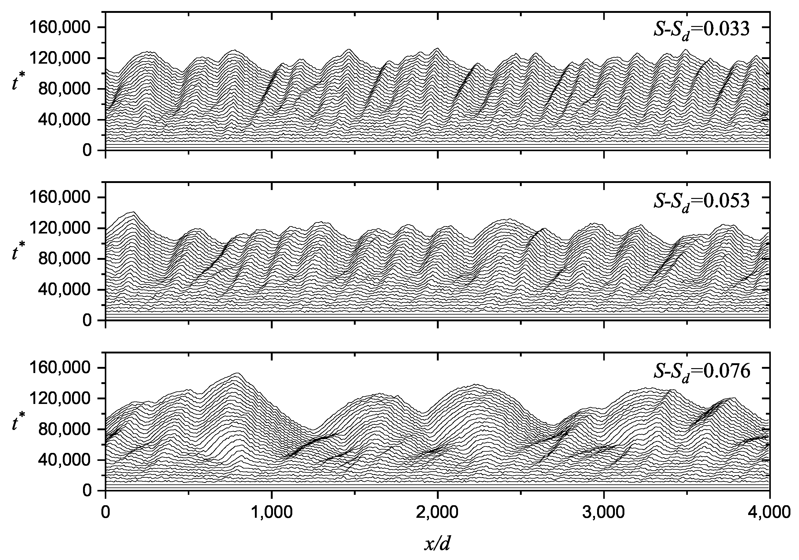
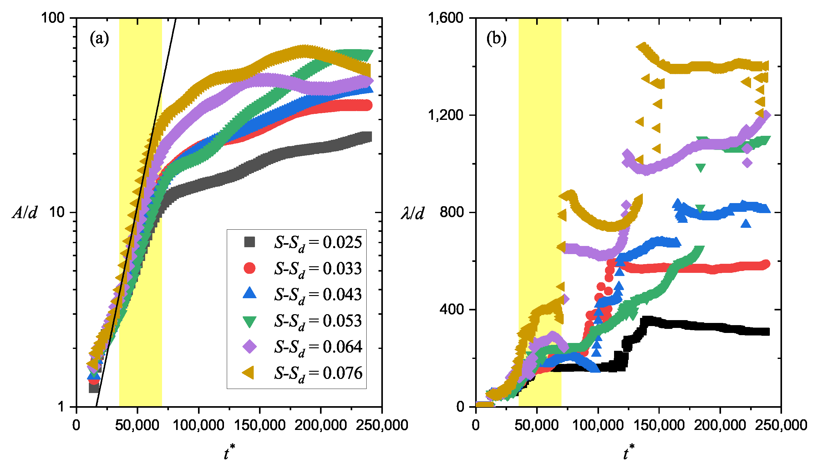
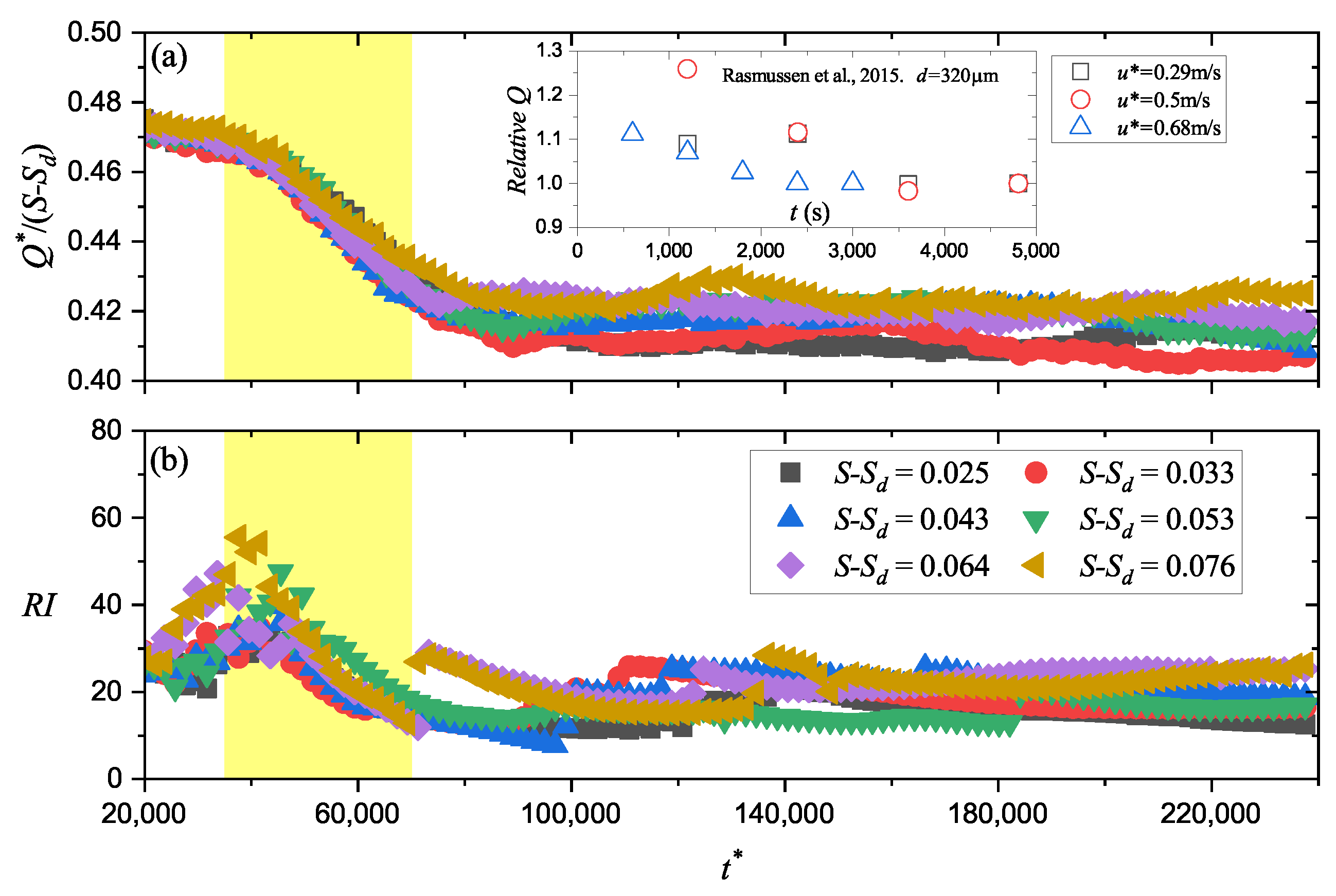
3.1. The Sand Flux Variation During Ripple Formation

Using the numerical method described above, we first simulated the development of the ripple surface and checked the consequent sand flux variation. It is worth mentioning that in this work we used monodisperse particles to avoid the influence of the particle size distribution. The size of the computational domain was $x\times y\times z=4000d\times 40d\times 1200d$, and the boundary condition was periodic in the x and the y direction. With $\widehat{g}=g\left(1-{\rho }_f/{\rho }_p\right)$, the Shields number $S={\rho }_f{u}^{*2}/\left({\rho }_p\widehat{g}d\right)$ in all cases ranged from 0.017 to 0.095. Here, we kept S below 0.1, because according to references [19,27,28], for larger Shields number S, the relationship between sand flux Q and S will no longer be linear. The range of S for which the linear scaling law $Q\propto S$ becomes invalid is called the Bagnold-like region. In this region, the average velocity of the particles in the air is not only related to the particle’s dynamic thresholds (threshold Shields number $S_d$ or threshold friction velocity $u_d^{*}$—they correspond to the smallest wind strength that can maintain the particle transport) but also controlled by the velocity of particles flying above the transport layer [29]. Except for the Shields number, particle transport can be influenced by the other two dimensionless numbers, which are the density ratio $s={\rho }_p/{\rho }_f$ and the Galileo number $Ga=\sqrt{s\widehat{g}{d}^3}/\nu$. For the subsequent simulations, we fixed these two parameters as $s=2098$ and $Ga=38$.

At the beginning of our simulations, the sand particle transport was triggered by randomly distributed inducing particles. These particles arouse other resting grains from the surface causing chain reactions and eventually leading to a saturated sand flux. Before calculating ripple development, we reserved enough time ($t^{*}=t/\sqrt{d/\widehat{g}}$ from 0 to 12,000) for the system to saturate. Equation (15) was unused during this time, and the sand flux rapidly reached to a steady value. We used this procedure to make sure that the following sand flux variation was only caused by the surface deformation. Then, the surface started to deform. As the space–time diagrams show in Figure 2, small bumps emerged from the sand bed regularly and migrated slowly in the wind direction. It is obvious that the wavelength ($\lambda$, the horizontal distance from crest to crest) and the amplitude (A, the vertical distance from trough to crest) of ripples grew with time. To have a clearer look at the morphological development of sand ripples, we calculated the autocorrelation $C_a\left(\Delta \lambda ,t\right)=〈z\left(x,t\right)z\left(x+\Delta \lambda ,t\right)〉-{〈z\left(x,t\right)〉}^2$ of the ripple profiles and averaged the results over the y direction. Then, the average amplitude was calculated from $A\left(t\right)=2\sqrt{2C_a\left(0,t\right)}$, and the average wavelength $\lambda \left(t\right)$ corresponds to the x-coordinate of the first peak on $C_a\left(\Delta \lambda ,t\right)$. As the results show in Figure 3, the ripple wavelength and the amplitude both increased with time. Moreover, the growth rate became more and more insignificant, and it eventually became zero at the fully developed state of the aeolian sand ripples.

As the bright yellow background demonstrates, in Figure 3a, there was a stage where the ripple amplitude grows exponentially. It is called the initial stage. Former works [19,30] have proved that before this stage ($t^{*}<$ 35,000 in this work), the bed surface is noticeably three-dimensional. Small bumps emerge from the surface at an arbitrary location. These bumps grow in the transverse direction and link to each other. Eventually, they become the primitive form of aeolian sand ripples. Then, because of the symmetrical ripple form, the bed surface no longer varies in the y direction. More and more low-energy particles tend to climb along the stoss slope of the sand ripple causing an exponential growth on the amplitude. From theoretical analyses, we have already known that this exponential-increase amplitude comes from the first-order contribution of the wavy bed surface [11,12,15]. The most unstable mode of the surface profile caused by this contribution represents the initial wavelength, which corresponds to the first plateau of the wavelength in Figure 3b. Then, after the initial stage ($t^{*}>$ 70,000 in this work), coarsening takes place. It makes adjacent bumps merge to each other. We can see there was a continuous growth of the ripple wavelength in the initial stage and a subsequent step growth in the coarsening stage. The later abrupt wavelength growth was caused by merging ripples.

Next, we checked the sand flux variation during ripple formation. In this work, the horizontal sand flux Q was calculated as the average horizontal particle momentum per unit bed area, i.e., $Q={〈{\sum }_N{m}_p{v}_x〉}_T/\Delta$, where N is the particle number in the air; $\Delta$ is the bottom area of the entire computation domain; and ${〈.〉}_T$ represents the time average. We nondimensionalized Q via $Q^{*}=Q/\left({\rho }_{p}d\sqrt{s\widehat{g}d}\right)$. The temporal evolution of $Q^{*}$ in different wind strengths is shown in Figure 4a. According to former experimental and numerical works [19,31,32,33], we have already known that there is a linear relationship between Q and the Shields number S. Thus, instead of $Q^{*}$, here we checked $Q^{*}/\left(S-S_d\right)$ to reveal more information. It is worth mentioning that the threshold $S_d$ used here was evaluated at $t^{*}=$ 20,000. As the result shows, $Q^{*}$ holds a relatively stable value in the beginning of bed deformation. Then, an obvious decrease happens within the initial stage of the ripple formation. After the initial stage, a new stable value of $Q^{*}$ was reached. Except the decrease in sand flux, we noticed $Q^{*}/\left(S-S_d\right)$ derived from different wind strengths no longer coincided to each other after the initial stage. This can be caused by two possibilities: (a) $S_d$ varies during the initial stage or (b) the relationship between $Q^{*}$ and $S-S_d$ is not linear on the ripple surface. The latter is less likely to be true, because as we know, the linear relationship has already been proved by many experiments, which are always performed on ripple surface.

We also checked the temporal development of the ripple index ($RI=\lambda /A$) in Figure 4b and found $RI$ increases until the initial stage begins. One needs to be aware that the value of $RI$ does not represent the ratio between $\lambda$ and A before the initial stage. Because as mentioned before, the typical ripple form has not emerged at this time. Thus, the increase in $RI$ in this stage represents nothing, and the flux was unrelated to this variation until the initial stage. The sand ripple started to grow in the initial stage. $RI$ decreased in this stage, which is similar to Q. This decrease lasted to the end of the initial stage, when $RI$ and Q all reached to a relatively stable value. However, according to Figure 3, $\lambda$ and A held their increase after the initial stage. Thus, combining all the results, we can draw a conclusion that Q is controlled by the ripple index $RI$. Additionally, we noticed that the final $RI$ derived from our model was about 20. This coincides with the results from wind tunnel experiments and field observations [1,7,9,10]. However, they have not revealed the decrease in $RI$ within the initial stage.

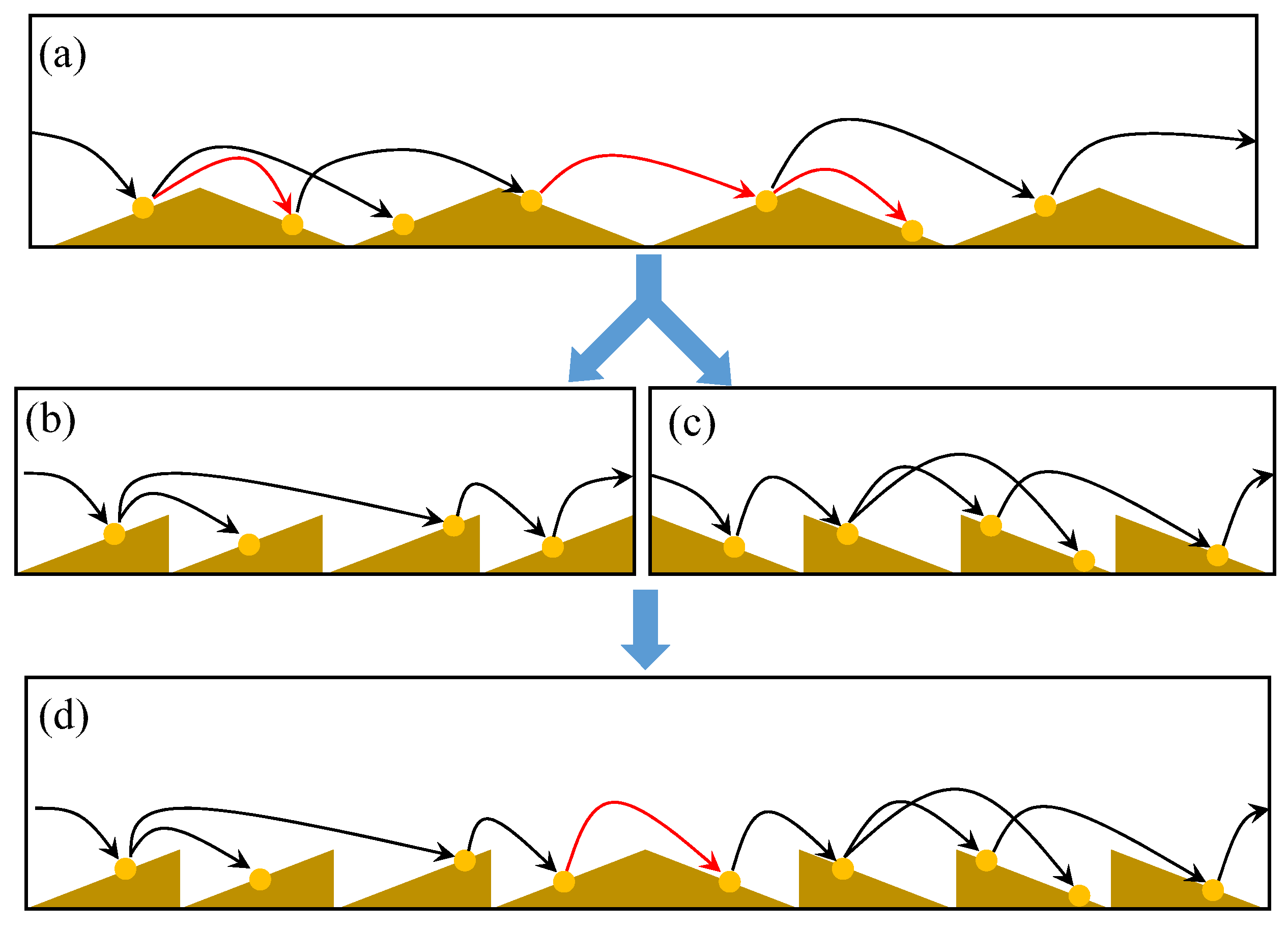
3.2. The Relationship between the Sand Particle Transport and the Ripple Index

To perform further studies on the relationship between Q and $RI$, we ran several extra cases with pre-rippled sinusoidal wavy surfaces (triangular wavy surfaces and sinusoidal wavy surfaces showed no differences on the result). For all the cases, the amplitude A was set as $8d$, which is observed in Figure 3a as a typical amplitude within the initial stage. The wavelength varies from $50d$ to $1000d$, making the ripple index $RI$ range from 6.25 to 125. The study on the situations with $RI<15$ was necessary, because for some specific conditions, the sand bed will develop to mega ripples, which has a much smaller ripple index [34]. For every pre-rippled simulation case, the code module that contains Equation (15) is disabled, and we reserved enough time for all the cases to ensure them to reach the saturated state. This procedure helped us to strictly control the value of $RI$. To derive authentic results, for all the pre-rippled cases, the density ratio s was set between 1325 and 5300; $Ga$ ranged from 27 to 60; and S varied from $0.01$ to $0.1$. The other settings were the same as the settings of the ripple formation cases mentioned before.

We first tried to simplify the problem. As Figure 5a shows, reptating particles and saltating particles bounced forward along the wavy bed surface. There are two typical movement modes for them. One is hopping from a stoss slope to another stoss slope or from a lee slope to another lee slope (black lines in Figure 5a demonstrate this kind of particle trajectories); the other one is hopping from a stoss slope to a lee slope or from a lee slope to a stoss slope (red lines in Figure 5a demonstrate this kind of particle trajectories). We defined the former trajectories as monotone trajectories and defined the latter as non-monotone trajectories. As Figure 5b,c shows, if all the particles have monotone trajectories and if we only study the ensemble average results, the whole system can be estimated by the combination of two simpler sub-systems, which only have a stoss slope or a lee slope. The particle with a non-monotone trajectory can be considered as a link, which transmits energy between the system shown in Figure 5b,c. We checked this energy-transmitting capability by counting the particle number that impacts the surface or take-off from the surface. $N_{stoss}^{in}$ represents the total number of impact particles that hit the stoss slope, and $N_{stoss}^{out}$ represents the total number of the particles take-off from the stoss slope. Similarly, we also had $N_{lee}^{in}$ and $N_{lee}^{out}$ for the lee slope. We checked $N_{lee}/N_{stoss}$ for the impact and take-off particles, because this ratio was useful for the subsequent studies. In Figure 6, we found $N_{lee}^{in}/N_{stoss}^{in}$ decreased linearly with 1/RI, meanwhile, $N_{lee}^{out}/N_{stoss}^{out}$ decreased quadratically. These decreased relationships are all independent to the wind strength and the particle/fluid properties. Moreover, there was a difference between these two ratios, which is demonstrated by the bright yellow shade. This difference was due to the contribution of the non-monotone particle trajectories. Because if all particles have monotone trajectories, we can easily derive $N_{stoss}^{out}=N_{stoss}^{in}$ and $N_{lee}^{out}=N_{lee}^{in}$. This yields an expression

$$N_{lee}^{in}/N_{stoss}^{in}=N_{lee}^{out}/N_{stoss}^{out}=r_a,$$

(16)

where we defined this ratio as $r_a$. To continue our study, we adopted this simplification. For simplicity, we assumed $r_a$ can be described by the linear fit of all the results in Figure 6, which is demonstrated as the dashed line. Thus,

$$r_a=-{\Gamma }_a\frac{1}{RI}+1,$$

(17)

where ${\Gamma }_a=5$ is a constant that will not change with the wind strength or the particle/fluid properties.

Similar to the definition of Q, we defined the particle transport load $M={〈{\sum }_N{m}_p〉}_T/\Delta$ to represent the average total mass of particles transported above the bed surface per unit bed area. As Figure 5 shows, we separated the whole system to two sub-systems. It is worth mentioning that these two sub-systems are not totally independent to each other. They share the same wind field. For a better understanding, one can imagine that we used the result derived from Figure 5d to estimate the result in Figure 5a. The former only has a few neglectable non-monotone trajectories in the middle. In the following work, for the particles interacting with the stoss slope, we used subscript s to represent their statistical quantities. For the particles interacting with the lee slope, we used subscript l. Then, we could write the stress balance on the bed surface [35]

$$-P_{zx}=\tau -{\tau }_{fw}-M_{s}gsin{\alpha }_s+M_{l}gsin{\alpha }_l,$$

(18)

$$P_{zz}=M_s\widehat{g}cos{\alpha }_s+M_l\widehat{g}cos{\alpha }_l,$$

(19)

where $P_{zx}$ and $P_{zz}$ are horizontal and vertical grain-born stress applied on the bed surface, respectively. They arose from inter-particle or particle-bed contacts. ${\alpha }_s$ and ${\alpha }_l$ are slope angles. We assumed ${\alpha }_s={\alpha }_l=\alpha$. $\tau =\rho u^{*2}$ is the air-borne shear stress far away from the bed surface; ${\tau }_{fw}$ is the air-borne shear stress on the bed surface. According to the drag partitioning theory [36], for a saturatde wind-driven particle transport system, ${\tau }_{fw}={\tau }_d$, where ${\tau }_d=\rho u_d^{*2}$ is the shear stress corresponding to the dynamic threshold. Moreover, recall the definition of $r_a$ in Equation (16); we find it can also represent the ratio of M, i.e., $M_l/M_s=r_a$. Use $M=M_l+M_s$, and define a parameter ${\mu }_b^0=-P_{zx}/P_{zz}$. Then we can derive

$$M^{*}=\frac{S-S_d}{{\mu }_b^{0}cos\alpha -\frac{s}{s-1}\frac{r_a-1}{r_a+1}sin\alpha }=\frac{1}{{\mu }_b}\left(S-S_d\right),$$

(20)

where $M^{*}=M/\left({\rho }_{p}d\right)$ is the dimensionless form of M; ${\mu }_b={\mu }_b^{0}cos\alpha -$$ssin\alpha \left(r_a-1\right)/$$\left(s-1\right)/\left(r_a+1\right)$. It shows a linear relationship between $M^{*}$ and S. From the simulation results shown in Figure 7, we proved that $M^{*}\propto S$ always holds for different $RI$, different s, and different $Ga$. Additionally, we found ${\mu }_b$ is obviously influenced by $RI$. The weak effect from s can be observed from the result, as well. To obtain the relationship between ${\mu }_b$ and $RI$, we used $\alpha ={cot}^{-1}\left(RI/2\right)$ to roughly estimate the slope angle. Then, we have

$${\mu }_b=\frac{1}{\sqrt{1+\frac{4}{{RI}^2}}}\left({\mu }_b^0-\frac{s}{s-1}\frac{2{\Gamma }_a}{{\Gamma }_{a}RI-2{RI}^2}\right),$$

(21)

which is derived from Equations (17) and (20).

As Figure 7 shows, not only ${\mu }_b$ varies with $RI$; $S_d$ also has a relationship with $RI$. According to the $S_d$ expressions on the slope [28], we similarly scaled $S_d$ as

$$S_d=\left(cos\alpha -\frac{s}{s-1}\frac{r_a-1}{r_a+1}\frac{sin\alpha }{{\mu }_b^0}\right)S_d^0=\frac{S_d^0}{\sqrt{1+\frac{4}{{RI}^2}}}\left(1-\frac{1}{{\mu }_b^0}\frac{s}{s-1}\frac{2{\Gamma }_a}{{\Gamma }_{a}RI-2{RI}^2}\right).$$

(22)

Noticing that for the flat surface situation, $RI$ becomes an infinitely great value, which leads to ${\mu }_b={\mu }_b^0$ and $S_d=S_d^0$. Thus, according to Equations (20) and (21) with $1/RI=0$, we can directly derive $S_d^0$ and ${\mu }_b^0$ from our flat surface results. It is worth mentioning that the “flat surface” here refers to the bed surface before the initial stage in the ripple formation simulation cases.

For the cases with $s=2098$ and $Ga=38$, we display the relationship between ${\mu }_b$ and $RI$ in Figure 8a. ${\mu }_b$ decreased with $RI$, and the decrease rate dropped rapidly. ${\mu }_b$ became more and more close to ${\mu }_b^0$ as $RI$ increased. The relationship between $S_d$ and $RI$ had the similar rule (Figure 8b). What was different was that the $S_d$ first dropped to a value smaller than $S_d^0$ at a large $RI$. Then, as $RI$ continued growing, it gradually increased to the value close to $S_d^0$. With derived ${\mu }_b^0$ and $S_d^0$, the results of Equations (21) and (22) are also shown in Figure 8 as the solid lines. Both of them roughly fit the simulation results, but Equation (22) cannot reflect the overly large decrease in $S_d$.

$RI=20$ is the typical ripple index of the fully developed aeolian sand ripples on earth [2,9,10]. According to our results, what varies most from the flat surface to $RI=20$ is not the dynamic threshold $S_d$ but the parameter ${\mu }_b$. So, we can say ${\mu }_b$ is a parameter that reflects the bed surface geometry. Substituting Equations (21) and (22) into Equation (20), we obtained a brief expression of $M^{*}$

$$M^{*}=\frac{1}{{\mu }_b^0}\left(S_r-S_d^0\right),$$

(23)

where, $S_r=S/\left\{1-2s{\Gamma }_a/\left[{\mu }_b^{0}RI\left(s-1\right)\left({\Gamma }_a-2RI\right)\right]\right\}$.

Finally, we checked the relationship between $M^{*}$ and $Q^{*}$. As Figure 9 shows, with specific s and $Ga$, for all the Shields numbers studied in this work ($S<0.1$), their relationship was close to linear. It is interesting that the ripple bed surface barely influenced the result. No obvious variations were observed between the results that corresponded to different $RI$. Thus, the relationship $Q^{*}\propto S-S_d$ was still valid for the sand particle transport upon the ripple surface. What was different from the result on the flat surface was the dynamic threshold $S_d$, and the proportionality coefficient between $Q^{*}$ and $S-S_d$ were controlled by the bed surface. According to Equation (23), we can also scale $Q^{*}$ as

$$Q^{*}\propto S_r-S_d^0.$$

(24)

Using this expression, we can estimate the relative quantity of the sand flux decrease during aeolian sand ripple formation in wind tunnel experiments. On the flat surface, the dynamic threshold $u_d^{*}$ can be estimated as $u_d^{*}=0.8u_t^{*}$ [1,37]. $u_t^{*}$ is the static threshold, and it can be calculated by $u_t^{*}=\sqrt{0.0123\left[sgd+3\times {10}^{-4}/\left({\rho }_{f}d\right)\right]}$ [26]. Then, we can derive $S_d^0$. We used $Q_0$ to represent the sand flux on flat surface. We easily derived $Q/Q_0=\left(S_r-S_d^0\right)/\left(S-S_d^0\right)$. We chose five common $RI$, which varied from 10 to 30. These $RI$ represent different aeolian sand ripples that emerged in wind tunnel experiments. Figure 10 exhibits the relationship between $Q/Q_0$ and S for a specific particle diameter d = 250 μm. One can find that for a specific ripple index, the sand flux caused by small wind strength is easier to be influenced by the ripple surface. $Q/Q_0$ rapidly approached to a constant value that was smaller than 1 when the wind strength increased. To have a clearer look, we extracted the $Q/Q_0$ values that correspond to $S=0.01$ and $S=0.1$. As shown in the inset of Figure 10, $Q/Q_0$ at these two wind strengths all increased with $RI$. For all the $RI$, the ripple bed was more influential to the sand flux in the situations with smaller wind strength. This coincides to the experiment result shown in the inset of Figure 4a.

4. Conclusions

Wind tunnel experiments reported a sand flux decrease during the long-term sand particle transport developments. In this work, we related this decrease to the sand ripple formation at the bed surface. From the numerical simulation and the theoretical analysis, we derived four main conclusions in this work:

• We simulated the emergence and development of aeolian sand ripples and found an obvious decrease in the ripple index $RI$ at the initial stage of ripple formation. This $RI$ variation coincides to a sand flux drop, indicating a strong connection between them.
• Particle transport load M decreased with $RI$. Its linear relationship with S always holds; only the proportionality coefficient ${\mu }_b$ of this relationship and the dynamic threshold $S_d$ varied with $RI$. We derived their expressions in Equations (21) and (22).
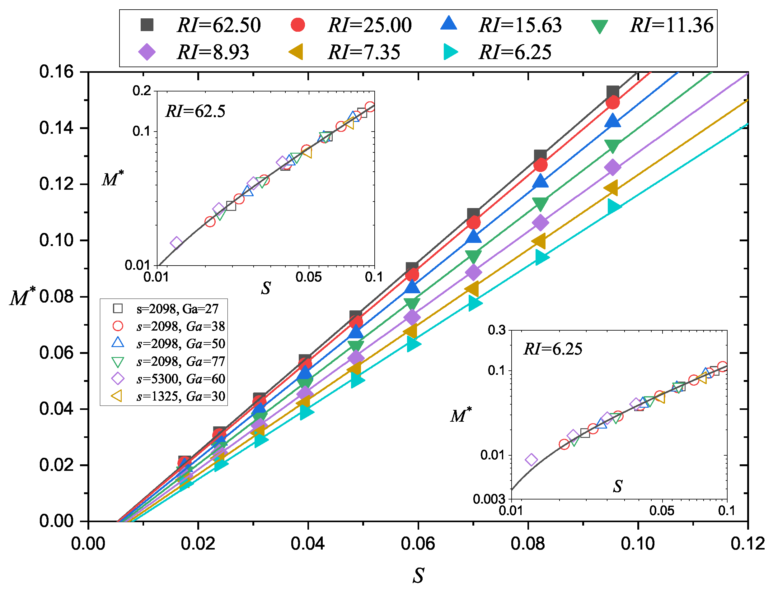
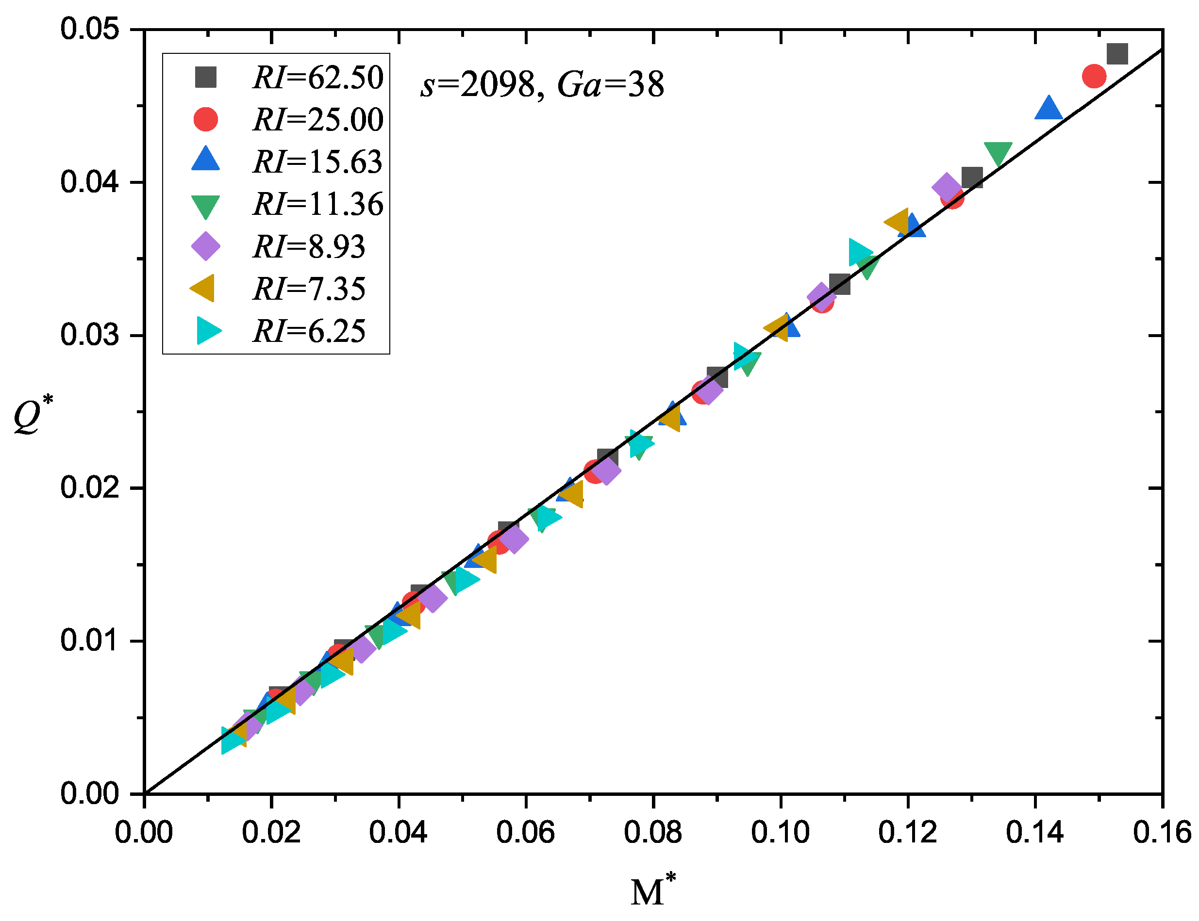
• The relationship between M and the sand flux Q was barely influenced by $RI$. For the S smaller than 0.1, we roughly had $Q\propto M$.
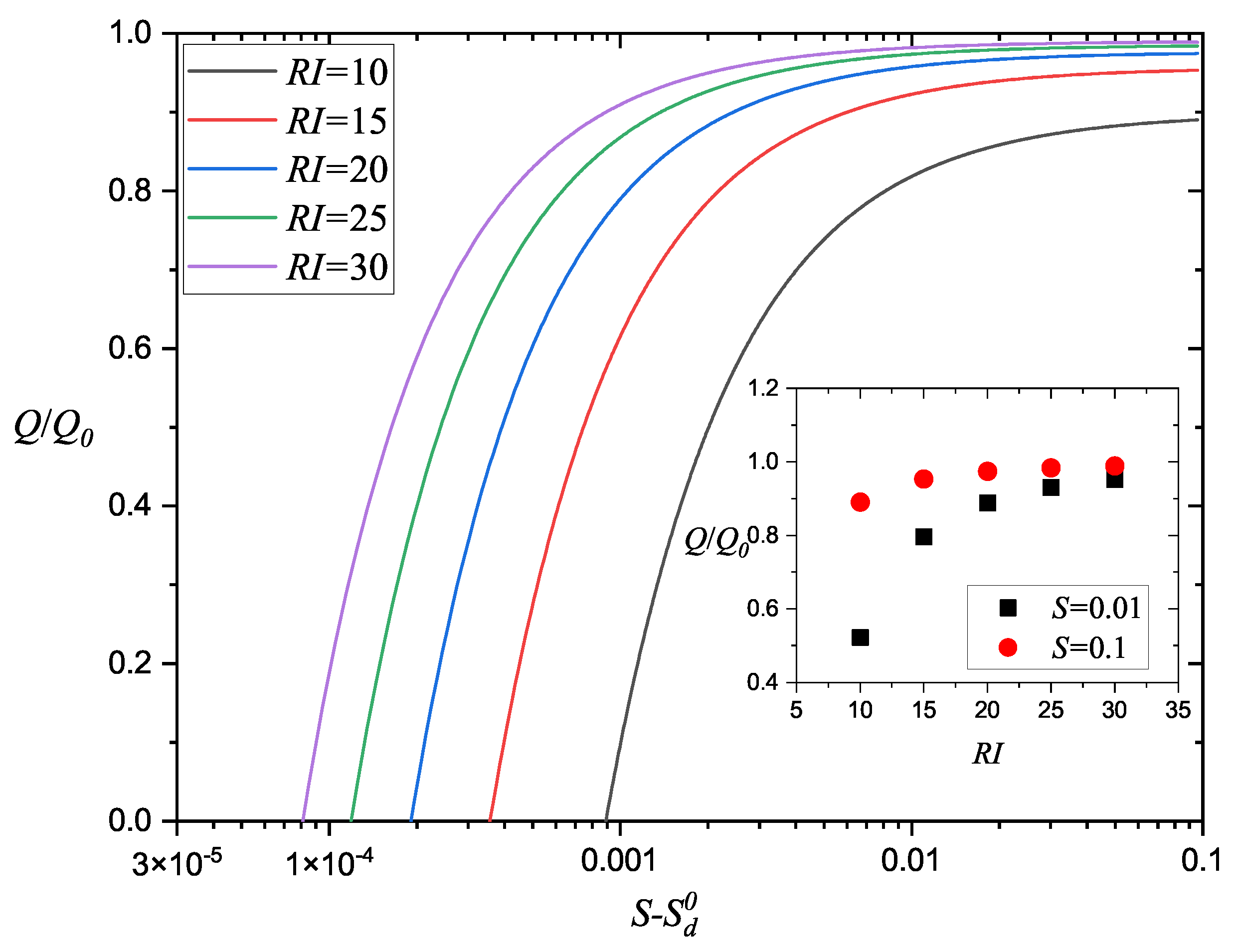
• We presented the relationship between Q, S, and $RI$ in Equation (24). From this expression, we found the sand flux Q derived at the ripple surface was always smaller than that on the flat surface. A larger $RI$ corresponds to a smaller Q. Cases with small wind strength are easier to be influenced by the ripple bed.

With these conclusions, we finally explained why sand flux decreased during wind tunnel experiments. We hope this work could show some helpful ideas to future experiments. We learned that for some situations, while studying the sand transport, the sand ripple on the bed surface is no longer a neglectable tiny structure. Moreover, Equation (24) can be used for the field observations. By measuring the ripple index and the sand flux at two different wind strengths, one can derive the flat surface dynamic threshold $S_d^0$, which is a rough estimation of the local sand particle dynamic threshold. We need to do wind tunnel experiments in the future to verify this usage and to conduct a further improvement in the expression of Q.

References

1. Bagnold, R.A. Physics of Blown Sand and Desert Dunes; W. Morrow & Company: New York, NY, USA, 1941. [Google Scholar]
2. Yizhaq, H.; Balmforth, N.J.; Provenzale, A. Blown by wind: Nonlinear dynamics of aeolian sand ripples. Phys. D Nonlinear Phenom. 2004, 195, 207–228. [Google Scholar] [CrossRef]
3. Rasmussen, K.; Mikkelsen, H. Wind tunnel observations of aeolian transport rates. In Aeolian Grain Transport 1; Barndorff-Nielsen, O.E., Willetts, B.B., Eds.; Springer: Vienna, Austria, 1991; pp. 135–144. [Google Scholar]
4. Rasmussen, K.R.; Valance, A.; Merrison, J. Laboratory studies of aeolian sediment transport processes on planetary surfaces. Geomorphology 2015, 244, 74–94. [Google Scholar] [CrossRef]
5. Wang, X.; Zhang, C.; Huang, X.; Shen, Y.; Zou, X.; Li, J.; Cen, S. Wind tunnel tests of the dynamic processes that control wind erosion of a sand bed. Earth Surf. Process. Landf. 2019, 44, 614–623. [Google Scholar] [CrossRef]
6. Tong, D.; Huang, N. Numerical simulation of saltating particles in atmospheric boundary layer over flat bed and sand ripples. J. Geophys. Res. Atmos. 2012, 117, D16205. [Google Scholar] [CrossRef]
7. Sharp, R.P. Wind ripples. J. Geol. 1963, 71, 617–636. [Google Scholar] [CrossRef]
8. Walker, J.D. An Experimental Study of Wind Ripples. Ph.D. Thesis, Massachusetts Institute of Technology, Cambridge, MA, USA, 1981. [Google Scholar]
9. Andreotti, B.; Claudin, P.; Pouliquen, O. Aeolian sand ripples: Experimental study of fully developed states. Phys. Rev. Lett. 2006, 96, 028001. [Google Scholar] [CrossRef] [Green Version]
10. Schmerler, E.; Katra, I.; Kok, J.F.; Tsoar, H.; Yizhaq, H. Experimental and numerical study of Sharp’s shadow zone hypothesis on sand ripple wavelength. Aeolian Res. 2016, 22, 37–46. [Google Scholar] [CrossRef]
11. Anderson, R.S. A theoretical model for aeolian impact ripples. Sedimentology 1987, 34, 943–956. [Google Scholar] [CrossRef]
12. Hoyle, R.B.; Woods, A. Analytical model of propagating sand ripples. Phys. Rev. E 1997, 56, 6861. [Google Scholar] [CrossRef] [Green Version]
13. Prigozhin, L. Nonlinear dynamics of aeolian sand ripples. Phys. Rev. E 1999, 60, 729. [Google Scholar] [CrossRef] [Green Version]
14. Valance, A.; Rioual, F. A nonlinear model for aeolian sand ripples. Eur. Phys. J. B-Condens. Matter Complex Syst. 1999, 10, 543–548. [Google Scholar] [CrossRef]
15. Csahók, Z.; Misbah, C.; Rioual, F.; Valance, A. Dynamics of aeolian sand ripples. Eur. Phys. J. E 2000, 3, 71–86. [Google Scholar] [CrossRef] [Green Version]
16. Wang, P.; Zhang, J.; Huang, N. A theoretical model for aeolian polydisperse-sand ripples. Geomorphology 2019, 335, 28–36. [Google Scholar] [CrossRef]
17. Bo, T.L.; Xie, L.; Zheng, X.J. Numerical approach to wind ripple in desert. Int. J. Nonlinear Sci. Numer. Simul. 2007, 8, 223–228. [Google Scholar] [CrossRef]
18. Durán, O.; Claudin, P.; Andreotti, B. Direct numerical simulations of aeolian sand ripples. Proc. Natl. Acad. Sci. USA 2014, 111, 15665–15668. [Google Scholar] [CrossRef] [Green Version]
19. Huo, X.; Dun, H.; Huang, N.; Zhang, J. 3d direct numerical simulation on the emergence and development of aeolian sand ripples. Front. Phys. 2021, 9, 358. [Google Scholar] [CrossRef]
20. Durán, O.; Andreotti, B.; Claudin, P. Numerical simulation of turbulent sediment transport, from bed load to saltation. Phys. Fluids 2012, 24, 103306. [Google Scholar] [CrossRef] [Green Version]
21. Brilliantov, N.V.; Pöschel, T. Kinetic Theory of Granular Gases; Oxford University Press: Oxford, UK, 2010. [Google Scholar]
22. Schwager, T.; Becker, V.; Pöschel, T. Coefficient of tangential restitution for viscoelastic spheres. Eur. Phys. J. E 2008, 27, 107–114. [Google Scholar] [CrossRef]
23. Fohanno, S.; Oesterle, B. Analysis of the effect of collisions on the gravitational motion of large particles in a vertical duct. Int. J. Multiph. Flow 2000, 26, 267–292. [Google Scholar] [CrossRef]
24. Lämmel, M.; Dzikowski, K.; Kroy, K.; Oger, L.; Valance, A. Grain-scale modeling and splash parametrization for aeolian sand transport. Phys. Rev. E 2017, 95, 022902. [Google Scholar] [CrossRef] [Green Version]
25. Lämmel, M.; Kroy, K. Analytical mesoscale modeling of aeolian sand transport. Phys. Rev. E 2017, 96, 052906. [Google Scholar] [CrossRef] [PubMed] [Green Version]
26. Shao, Y.; Lu, H. A simple expression for wind erosion threshold friction velocity. J. Geophys. Res. Atmos. 2000, 105, 22437–22443. [Google Scholar] [CrossRef]
27. Nalpanis, P.; Hunt, J.; Barrett, C. Saltating particles over flat beds. J. Fluid Mech. 1993, 251, 661–685. [Google Scholar] [CrossRef]
28. Pähtz, T.; Durán, O. Unification of aeolian and fluvial sediment transport rate from granular physics. Phys. Rev. Lett. 2020, 124, 168001. [Google Scholar] [CrossRef] [PubMed] [Green Version]
29. Durán, O.; Claudin, P.; Andreotti, B. On aeolian transport: Grain-scale interactions, dynamical mechanisms and scaling laws. Aeolian Res. 2011, 3, 243–270. [Google Scholar] [CrossRef]
30. Anderson, R.S. Eolian ripples as examples of self-organization in geomorphological systems. Earth-Sci. Rev. 1990, 29, 77–96. [Google Scholar] [CrossRef]
31. Creyssels, M.; Dupont, P.; El Moctar, A.O.; Valance, A.; Cantat, I.; Jenkins, J.T.; Pasini, J.M.; Rasmussen, K.R. Saltating particles in a turbulent boundary layer: Experiment and theory. J. Fluid Mech. 2009, 625, 47. [Google Scholar] [CrossRef] [Green Version]
32. Ho, T.D.; Valance, A.; Dupont, P.; El Moctar, A.O. Scaling laws in aeolian sand transport. Phys. Rev. Lett. 2011, 106, 094501. [Google Scholar] [CrossRef]
33. Martin, R.L.; Kok, J.F. Wind-invariant saltation heights imply linear scaling of aeolian saltation flux with shear stress. Sci. Adv. 2017, 3, e1602569. [Google Scholar] [CrossRef] [Green Version]
34. Lämmel, M.; Meiwald, A.; Yizhaq, H.; Tsoar, H.; Katra, I.; Kroy, K. Aeolian sand sorting and megaripple formation. Nat. Phys. 2018, 14, 759–765. [Google Scholar] [CrossRef]
35. Pähtz, T.; Durán, O.; Ho, T.D.; Valance, A.; Kok, J.F. The fluctuation energy balance in non-suspended fluid-mediated particle transport. Phys. Fluids 2015, 27, 013303. [Google Scholar] [CrossRef] [Green Version]
36. Owen, P.R. Saltation of uniform grains in air. J. Fluid Mech. 1964, 20, 225–242. [Google Scholar] [CrossRef]
37. Carneiro, M.V.; Rasmussen, K.R.; Herrmann, H.J. Bursts in discontinuous Aeolian saltation. Sci. Rep. 2015, 5, 11109. [Google Scholar] [CrossRef] [PubMed] [Green Version]
Figure 1. A sketch of the main particle transport forms in the aeolian particle transport system.
Processes 10 00354 g001
Figure 2. The spatial–temporal evolution of aeolian sand ripples in different wind strengths.
Processes 10 00354 g002
Figure 3. Sand ripple amplitude (a) and wavelength (b) increase with time. Different colors represent different wind strengths. The bright yellow shades highlight the initial stage of the ripple formation. In (a), for the amplitude result corresponds to S S d = 0.076 , black line is the fit line within the initial stage representing an exponential growth.
Processes 10 00354 g003
Figure 4. Sand flux (a) and ripple index (b) varies with time during the ripple formation and development process. Different colors represent different wind strengths. The bright yellow shades highlight the initial stage. The inset in (a) shows the flux decrease observed in the wind tunnel experiment [4]. The relative Q is the flux normalized by the last observed flux value.
Processes 10 00354 g004
Figure 5. A sketch of our simplification procedure. Black lines represent monotone trajectories. Red lines represent non-monotone trajectories. (a) is the original system. (b,c) are systems that only contain the particles with monotone trajectories. (a) can be roughly approached by the combination of (b,c), which is shown in (d).
Processes 10 00354 g005
Figure 6. N l e e i n ( o u t ) / N s t o s s i n ( o u t ) varies with R I , where N l e e i n ( o u t ) / N s t o s s i n ( o u t ) is the ratio between the impact (take-off) particle number at the lee slope and that at the stoss slope. The black line is a linear fit of N l e e i n / N s t o s s i n . The red line is a quadratic polynomial fit of N l e e o u t / N s t o s s o u t . The dashed line is a linear fit for all the data. The bright yellow shade highlights the difference between the impact particle results and the take-off particle results, reflecting the influence from non-monotone trajectories.
Processes 10 00354 g006
Figure 7. The relationship between the particle transport load M * and Shields number S. For filled symbols, different colors correspond to different R I . For hollowed symbols in the insets, different colors correspond to different particle/fluid properties. Two insets show the results of two specific R I . All the solid lines represent linear fits.
Processes 10 00354 g007
Figure 8. μ b (a) and S d (b) decrease with ripple index. Dashed lines represent their values at flat surface. Solid lines represent the results derived from Equations (21) and (22), respectively. All the results are corresponding to the cases with s = 2098 and G a = 38 .
Processes 10 00354 g008
Figure 9. The relationship between Q * and M * . Different colors represent different ripple indexes. The result was derived from the cases with s = 2098 and G a = 38 . Solid line represents a linear fit.
Processes 10 00354 g009
Figure 10. The relationship between Q / Q 0 and the wind strength, where Q / Q 0 is the ratio between the sand flux on ripple surface to the one on the flat surface. Different line colors represent different ripple indexes. The inset shows how Q / Q 0 varies with R I . All the results are derived from Equation (24).
Processes 10 00354 g010
Publisher’s Note: MDPI stays neutral with regard to jurisdictional claims in published maps and institutional affiliations.