Study on the Erosion of Choke Valves in High-Pressure, High-Temperature Gas Wells

Abstract

During the process of gas production in high-pressure, high-temperature (HPHT) gas wells, the choke valve, as the most vital component of the surface control equipment, plays a significant role in regulating the output and reducing the fluid pressure to ensure the safety of surface gathering and transportation equipment. High-pressure, high-velocity fluid flow and solid-phase particles cause deterioration of the choke valve. With the enhancement of intelligent and digital oilfields, conventional choke valves have been progressively replaced by electric choke valves. Due to the complex structure of the throttle valve, the flow path and the velocity state of the fluid in the throttle valve, and the distribution law of the erosion fraction are quite distinctive from those in the ordinary throttle valve, meriting further research. In this paper, a simulation of computational fluid dynamics (CFD) was conducted to determine the effects of the pressure distribution, fluid state, divergent particle sizes, and sand volume on the erosion rate of the choke valve. Under various valve openings, the fluid state and the location of high-risk points can be ascertained. The large particle size (diameter greater than 6 mm) of sand and gravel is convenient for causing concentrated erosion in the position of the valve hole, which induces the channel diameter to expand. Fine silt sand (diameter from 0.1 mm to 1 mm) gives rise to relatively uniform abrasion to the choke’s current-facing surface. This study can optimize the layout of the choke valve and reduce the cost and number of switching wells, thereby decreasing the frequency of maintenance and the pressure fluctuation’s effect on the formation.

1. Introduction

The HT1 well is an HPHT gas well with a tectonic belt on the southern edge of the Dzungar Basin, with a depth of over 7000 m and a closing pressure of more than 120 MPa [1]. As the most essential component of the choke manifold, the choke valve takes part in regulating the output and reducing the fluid pressure to ensure the safety of ground gathering and of transportation equipment and personnel [2]. Choke valve erosion is unavoidable as a result of the high-pressure, high-velocity airflow and the erosion engendered by solid-phase particles. The disclosure of the choke valve’s erosion law significantly reduces erosion and optimizes the choke valve’s structure [3]. A number of researchers have examined this issue.

Paggiaro et al. [4] experimentally validated a three-dimensional computational fluid dynamics (CFD) throttling flow simulation model. CFD flow and sand grain tracking simulations demonstrate that the predicted flow parameters are consistent with the experimental data, and the simulations can accurately predict the location of erosion hotspots. Chang Z. et al. [5] took advantage of the RNG k-ε turbulence model to numerically calculate the dual disc check valve’s three-dimensional transient flow based on dynamic mesh technology. Tuladhar U. et al. [6] investigated how the nozzle exit diameter and the slope of the cut front affect gas flow behavior using the Reynolds averaged Navier–Stokes (RANS)-based k–ω turbulence model. Andres Pinilla et al. [7] presented a numerical study that describes the working principle of RCP valves in accordance with a computational fluid dynamics (CFD) analysis. However, this study did not address the erosion of choke valves with variable morphology in high-pressure, high-speed fluids.

To address the above deficiencies, this paper focuses on the erosion of the adjustable choke valves at different opening in HPHT gas wells. The flow in the choke valve at various opening degrees was simulated utilizing CFD software, and the influence of the particle size and the sand volume of solid-phase particles on erosion were simulated. It is crucial to maximize the choke valve’s structure, as this would reduce field expenses.

2. Numerical Simulation Model of Erosion

2.1. Flow Equation of Liquid Phase

The production of sand is one of the primary challenges associated with the development of HPHT gas wells. The choke valve is more susceptible to sand erosion. Moreover, the flow in the choke valve can be simplified to a gas–solid two-phase flow, where the gas phase is methane and the solid phase is the sand particles of the formation. Since the volume fraction of the solid phase in gas production is typically less than 5%, when utilizing the Fluent simulation, the gas phase can be regarded as a continuous phase and the solid phase can be regarded as a discrete phase.

The flow equations of the gas phase include the equation of continuity, the equation of momentum, and the equation of turbulence model. Specific forms of the equations are as follows [8,9,10]:

Equation of continuity:

$$\frac{\partial \mathsf{\rho }}{\partial \mathrm{t}}+\frac{\partial \left({\mathsf{\rho }\mathrm{u}}_{\mathrm{i}}\right)}{\partial {\mathrm{x}}_{\mathrm{i}}}=0$$

(1)

where $\mathsf{\rho }$ is the density of the gas (continuous phase) and ${\mathrm{u}}_{\mathrm{i}}$ is the velocity component parallel to the axis ${\mathrm{x}}_{\mathrm{i}}$.

Equation of momentum [11]:

$$\frac{\partial \left({\mathsf{\rho }\mathrm{u}}_{\mathrm{i}}\right)}{\partial \mathrm{t}}+\frac{\partial \left({\mathsf{\rho }\mathrm{u}}_{\mathrm{i}}{\mathrm{u}}_{\mathrm{j}}\right)}{\partial {\mathrm{x}}_{\mathrm{j}}}=-\frac{\partial \mathrm{p}}{\partial {\mathrm{x}}_{\mathrm{i}}}+\frac{\partial {\mathsf{\tau }}_{ij}}{\partial {\mathrm{x}}_{\mathrm{j}}}+\mathsf{\rho }\mathrm{g}+F_i$$

(2)

where p is the static pressure, ${\mathsf{\tau }}_{ij}$ is the viscous stress tensor, g is the acceleration of gravity, and $F_i$ is the generalized volumetric force.

RNG k-ε turbulence model calculation has an extensive range of applications due to its high accuracy. The model is suitable for the numerical calculation of gas well throttling, and its equations are as follows [8]:

$$\frac{\partial \left(\mathsf{\rho }k\right)}{\partial \mathrm{t}}+\frac{\partial \left({\mathsf{\rho }\mathrm{ku}}_{\mathrm{i}}\right)}{\partial {\mathrm{x}}_{\mathrm{i}}}=\frac{\partial [(\mathsf{\mu }+\frac{{\mathsf{\mu }}_t}{{\sigma }_k})\frac{\partial \mathrm{k}}{\partial {\mathrm{x}}_{\mathrm{j}}}]}{\partial {\mathrm{x}}_{\mathrm{j}}}+G_k+G_b-Y_m-\mathsf{\rho }\mathsf{\epsilon }$$

(3)

$$\frac{\partial \left(\mathsf{\rho }\mathsf{\epsilon }\right)}{\partial \mathrm{t}}+\frac{\partial \left({\mathsf{\rho }\mathsf{\epsilon }\mathrm{u}}_{\mathrm{i}}\right)}{\partial {\mathrm{x}}_{\mathrm{i}}}=\frac{\partial [(\mathsf{\mu }+\frac{{\mathsf{\mu }}_t}{{\sigma }_{\mathsf{\epsilon }}})\frac{\partial \mathsf{\epsilon }}{\partial {\mathrm{x}}_{\mathrm{j}}}]}{\partial {\mathrm{x}}_{\mathrm{j}}}+C_{1\mathsf{\epsilon }}\frac{\mathsf{\epsilon }}{\mathrm{k}}{C}_k-C_{2\mathsf{\epsilon }}\mathsf{\rho }\frac{{\mathsf{\epsilon }}^2}{\mathrm{k}}-C_{1\mathsf{\epsilon }}{C}_{3\mathsf{\epsilon }}\frac{\mathsf{\epsilon }}{\mathrm{k}}{G}_b$$

(4)

where $\mathrm{k}$ is the turbulent flow energy, ${\mathsf{\mu }}_t$ is the turbulence viscosity, $\mathsf{\mu }$ is the fluid dynamic viscosity, $G_k$ is the turbulent flow energy generated by the average speed gradient, $G_b$ is the turbulent flow energy generated by the buoyancy, $Y_m$ is the effect of the expansion of compressible turbulence fluctuation on the overall dissipation rate, ε is the turbulent flow energy consumption dissipation power, ${\sigma }_k$ is the turbulent kinetic energy k of the turbulent flow Plant number, and ${\sigma }_{\mathsf{\epsilon }}$ is the turbulent flow Plant number with an $\mathsf{\epsilon }$ dissipation rate [12].

The default values in Fluent are $C_{1\mathsf{\epsilon }}$ = 1.42, $C_{2\mathsf{\epsilon }}$ = 1.68, and $C_{3\mathsf{\epsilon }}$ = 1.83 [13,14,15].

2.2. Movement Equation of Particle Phase

Due to the small volume fraction of solid particles in the choke valve, particle collisions can be disregarded, and the DPM (Deformable Part Model) is adopted to simulate the erosion of solid particles.

The kinetic equation for particles in discrete phase models is as follows [16]:

$$\frac{d{u}_P}{\mathrm{dt}}=F_D\left(u-u_P\right)+\frac{\mathrm{g}\left({\rho }_P-\mathsf{\rho }\right)}{{\rho }_P}+F_P$$

(5)

where $u_P$ is the particle velocity component, ${\rho }_P$ is the particle density, $F_D$ is the flow resistance of the particle, and $F_P$ is other forces affected by the particle.

Other forces affected by the particles are as follows [17]:

$$F_D=\frac{{18}_{\mu }}{{\rho }_P{d}_P^2}\frac{C_{D}Re}{24}$$

(6)

$$\mathrm{Re}=\frac{\rho d_P\left|u-u_P\right|}{\mu }$$

(7)

where $d_P$ is the particle diameter, $\mathrm{Re}$ is the relative Reynolds number, and $C_D$ is the resistance coefficient.

2.3. Equation of Erosion

In the evaluation of the erosion of the choke valve, the erosion rate is selected for analysis and comparison; the DPM model is utilized for calculation; the flow equation is solved based on the Euler–Lagrange method, which considers gas as the continuous phase and solid particles as the discrete phase and the change in the particle’s state of motion is accounted for by a differential equation to obtain the particle motion trajectory and energy transfer change.

The erosion rate calculation model is as follows [18]:

$$R_{\mathrm{erosion}}={\displaystyle \sum }_{P=1}^N\frac{m_{P}C\left(d_P\right)f\left(\alpha \right)v^{b\left(v\right)}}{A_{\mathrm{face}}}$$

(8)

where $m_P$ is the average mass flow of the particles, which is a fixed value defined in the inlet face prior to the calculation; N is the number of particles when colliding with the wall of the structure; $C\left(d_P\right)$ is a particle diameter function, usually related to the physical properties of the material being eroded, and the value of $C$ is 1.8 × 10⁻⁹ [19,20] because the size of the particles in this paper is mono; $\alpha$ is the impact angle between the particle motion path and the wall surface of the structure; $f\left(\alpha \right)$ is the angle of the impact function of the particles; $v$ is the relative velocity of the particles; $b\left(v\right)$ is a function of the relative velocity of the particles, and the solid particles in this article are quartz sand, which take the value of 2.6 [21,22,23]; $A_{\mathrm{face}}$ is the wall area of the wall surface of the particle collision wall, which is defined during the process of simulation based on the effect of the angle and the velocity of the particles; and $R_{\mathrm{erosion}}$ is the erosion quality of the particles on the wall surface of the structure per unit area per unit time. The choke impact angle function $f\left(a\right)$ was proposed by Huser and Kvemvold.

When particles strike the valve, the speed of the particles decreases. To reflect the situation, the concept of recovery coefficient is put forward to describe the loss. The speed ratio of the vertical wall before and after the collision is a normal recovery coefficient ${\mathsf{\epsilon }}_n$, and the ratio of the tangent direction of the wall before and after the collision is the tangential recovery coefficient ${\mathsf{\epsilon }}_t$.

The equations proposed by A. Forder [24] are used to calculate the recovery coefficients. The expressions are as follows:

$${\mathsf{\epsilon }}_n=0.993-0.0307\mathrm{a}+4.75\times {10}^{-4}{a}^2-2.61\times {10}^{-6}{a}^3$$

(9)

$${\mathsf{\epsilon }}_t=0.998-0.029a+6.43\times {10}^{-4}{a}^2-3.56\times {10}^{-6}{a}^3$$

(10)

3. Model Creation with Parameter Setting

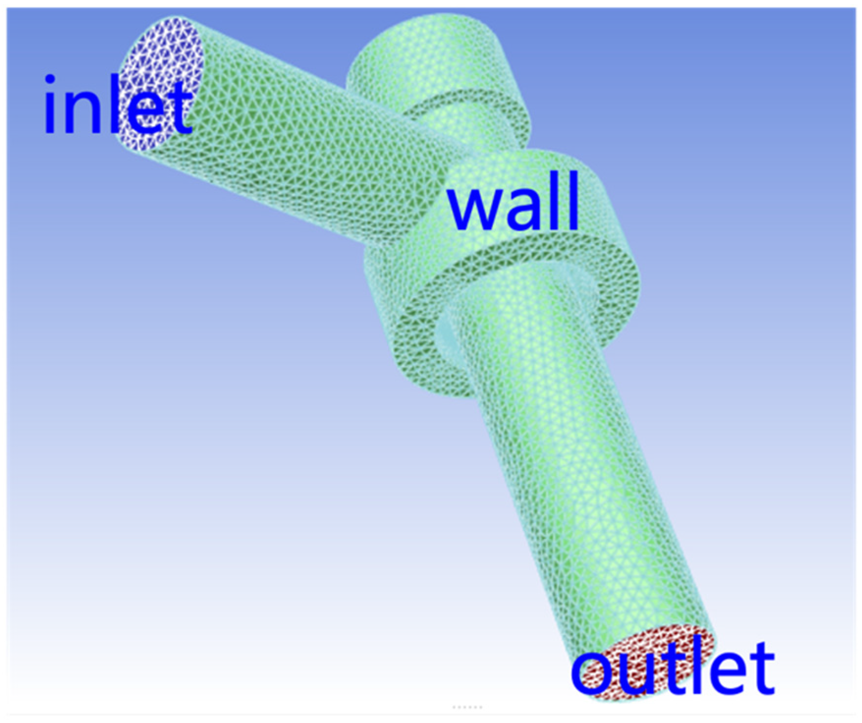
3.1. Choke Valve Geometry and Meshing

The choke valve modifies the opening degree by adjusting the tour valve’s position relative to the spool. Choke geometries are built by SOLIDWORKS, and the choke valve model consists of three parts: the spool, the base, and the valve. This is shown in Figure 1. The distinctive openings of the choke valve can be simulated by changing the position of the valve and the base. The combined structure is shown in Figure 2. Three rows of four holes with diameters of 3.2 mm, 6.5 mm, and 10.2 mm are staggered across the opening of the spool.

The structure of the combined choke valve is demonstrated in Figure 2.

The extraction of fluids is performed using the ANSYS geometry tools. The fluid model is based on a cylinder structure, and triangular meshing helps ensure the mesh’s quality.

3.2. Initial Boundary Condition Setting

The inflow surface, the outflow surface, and the contact surface of the inner wall of the fluid and the choke valve are characterized in the model, as revealed in Figure 3. Formulated using field data, the inlet pressure is set to 80 MPa, the temperature is set to 300 K, the outlet is set to outflow, and the particle state is set to escaping. Predicated on the geometric dimensions of the choke valve and the gas flow rate, the Reynolds number is determined to be 215,463, which is larger than 4000, indicating that the fluid’s flow state is turbulent. The grit is chosen to be calcium sulfate, with a density of 2400 kg/m³. The continuous phase in a high-pressure gas well is mainly methane, which is less dense, and the effect of gravity can be ignored. Furthermore, the energy equation states are open, avoiding standard wall functions, no-slip conditions, and particles bouncing off after collision avoidance. The amount of momentum reduction is determined by the collision model. Thus, the solution method adopts the SIMPLE algorithm to solve the pressure–velocity coupling, the others adopt the second-order windward format, and the mean residual convergence standard is set to the recommended value of 10⁻⁵. High temperature and high pressure frequently occur together, and a high pressure generally indicates a high rate of gas well production. The change in pressure and flow directly affects the quantity of the fluid and particles impacting the nozzle wall. In comparison to a low flow rate, erosion at a high flow rate is more noticeable and causes bigger priority at the production sites. The simulation and conclusions in this paper are more applicable to high-pressure and high-production gas wells.

3.3. Mesh Independence Verification

The mesh independence verification of the fluid domain model in the choke valve is carried out. A too-large grid will lead to large errors or non-convergence of the calculation results, while too dense of a grid will increase the burden of calculation. Under the premise of ensuring the accuracy of the simulation results, the selection of an appropriate mesh size can therefore reduce the cost of calculation. Using the Ansys Fluent software, the erosion wear rate is the statistical average, and the grid independence verification is conducted with the maximum erosion rate as an indicator. The consequence is shown in Figure 4. Under the condition that the number of grids reaches 56,734, the calculation results tend to be stable, and hence, the number of grids is applied in subsequent numerical simulation calculations.

4. Choke Valve Erosion Numerical Simulation

4.1. Pure Gas Phase Erosion

The fluid is set to be pure methane without the addition of solid-phase particles, simulating the situation inside a choke valve with a pure gas phase.

4.1.1. Wall Pressure Distribution

The distribution of the pressure in the choke valve is simulated as shown in Figure 5.

By observing the pressure of the wall, the pressure distribution of the choke valve’s wall can be obtained. It does seem that the high pressure is located on the outer wall of the spool facing the fluid. A high pressure indicates stronger gas erosion, and the presence of sand can exacerbate erosion at this location, which is a high-risk location that deserves additional attention. Broadly speaking, the pressure on the inner wall of the spool is low, and its erosion is considerably weaker than the outer wall erosion.

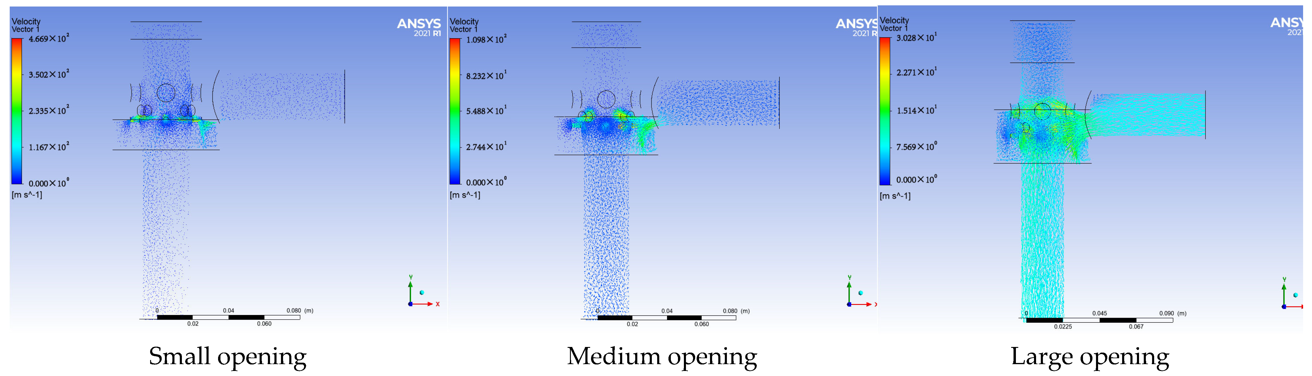
4.1.2. Velocity Vectors at Different Openings

In comparison to the traditional choke valve, the adjustability of the cage and sleeve choke valve’s opening is its most prominent characteristic. This signifies that in divergent production systems, the structure of the choke valve is divergent, the flow of the fluid is dissimilar, and the inner wall pressure and the highest point of the fluid speed differ significantly. By simulating the distribution of the inner wall pressure of the choke valve under different opening degrees, it is possible to determine the distribution of high-risk sites under various production systems. Velocity vector distribution at different openings are shown in Figure 6.

Small opening: The erosion position is concentrated in the small hole position in the direction of the incoming flow, and while the other three holes also have an erosion phenomenon, the degree of erosion is lighter than the small hole in the incoming flow position.

Medium opening: The erosion position is concentrated along the flow direction of the small and middle holes, while the other three small holes do not show erosion. It should be noted that there is a phenomenon of fluid acceleration in the presence of the narrow slits in the middle hole, which can result in more serious erosion.

Large opening: The erosion position is concentrated in the flow direction of the large hole and the middle hole, and the small hole does not show erosion.

By simulating the distribution of the velocity vector at different openings, the shear stress of the choke valve wall surface can be reflected. It is also possible to recognize the erosion of the choke valve from a distinctive angle. Since the sand is wrapped in gas and moves, the velocity vector of the fluid can show the movement of the gravel to a certain extent. Through the simulation described above, the high-risk locations corresponding to each of the small, medium, and large openings are determined, allowing for the use of harder materials in the manufacture of choke valves.

4.2. Simulation of Sand Erosion

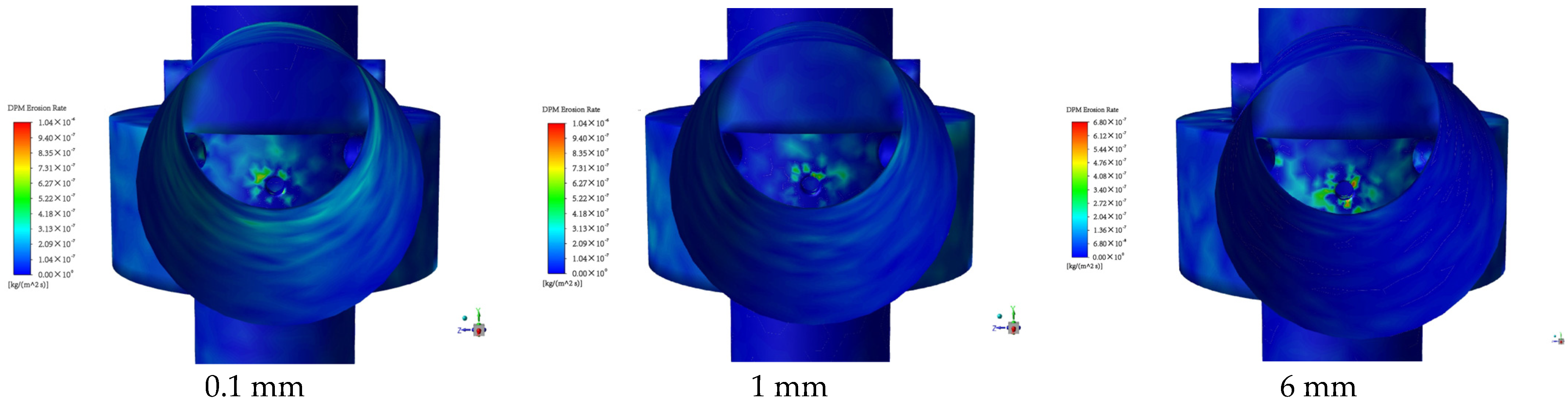
4.2.1. Effect of Gravel Diameter on Wear

In the case of a certain amount of grit, the erosion of the wall surface of the choke valve under dissimilar gravel diameters is simulated, and the consequences are shown in Figure 7.

In fine silt sand with a gravel diameter of 0.1 mm, the erosion area on the incoming flow surface of the valve’s spool part is more uniformly distributed, and the phenomenon of erosion is in a larger area. As the particle size of the gravel increases, the erosion position shifts towards the edge of the hole and the erosion area shrinks, converging around the small hole. Consistent with the actual performance in the field, when there are large particles of gravel, the erosion at the small hole is very severe and concentrated at the small hole runner; eventually, the small hole continuously expands, resulting in a change in the throttling effect, and the yield and pressure after throttling have a gradual increase. Due to the fact that the high-pressure gas well generally adopts a secondary throttling, the first-level throttling will block off the large particles of sand and gravel, and only fine silty sand exists at the secondary choke. The erosion of the first-level choke valve is significantly larger than that of the secondary choke valve, indicating that the grit of the large particles has a greater impact on the erosion process.

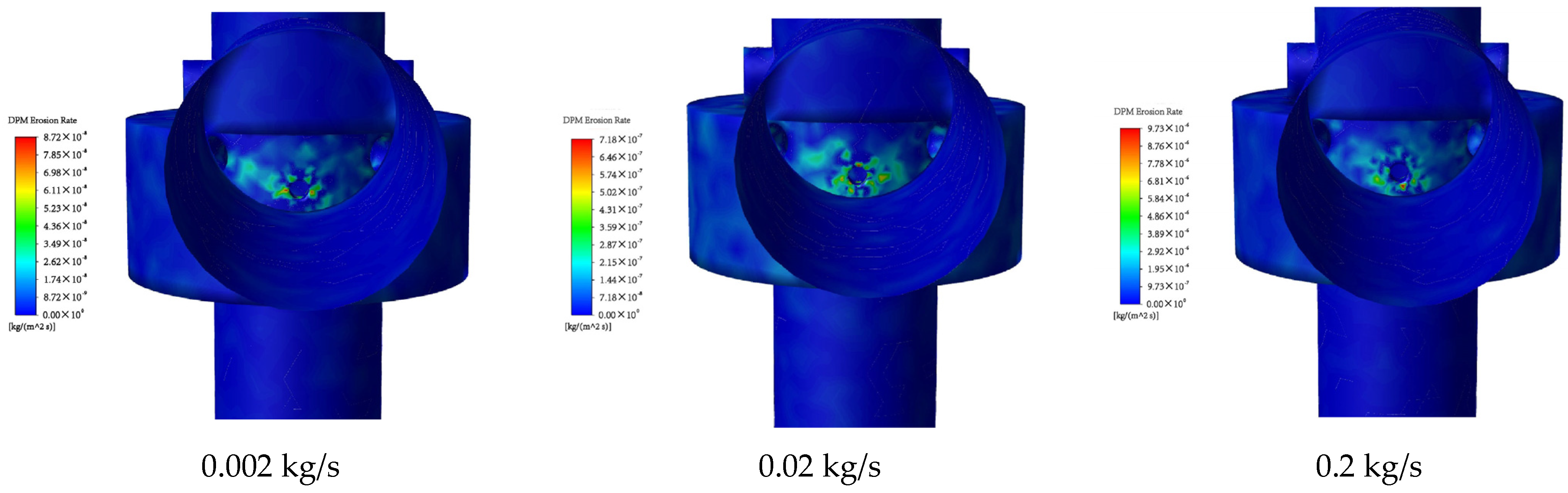
4.2.2. The Influence of Sand Volume on Wear

The diameter of the gravel is set at 0.1 mm, which can simulate fine silt sand. A simulation of the outcomes is depicted in Figure 8 using varying sand quantities.

The maximum erosion rates of 0.002 kg/s, 0.02 kg/s, and 0.2 kg/s are 8.72 × 10⁻⁸, 7.18 × 10⁻⁷, and 9.73 × 10⁻⁶, respectively. The erosion velocity of the choke valve spool surface is within an order of magnitude, and the maximum erosion speed point is randomly distributed around the pore size. The erosion is uniform and correlates positively with the amount of sand produced. The results show that, in the case of fine silt sand, the erosion is positively correlated with the amount of sand, the distribution of the erosion locations does not change, and all of them are more commonly abraded.

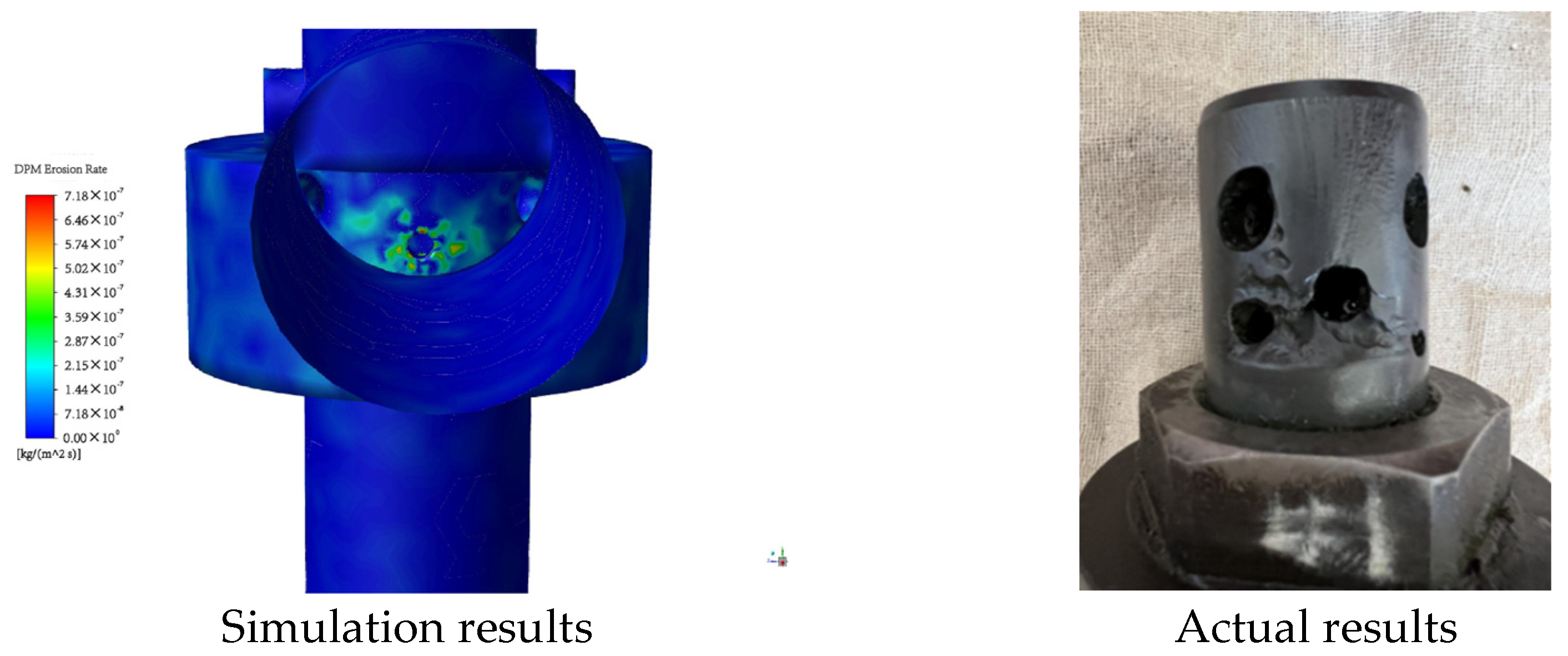
4.3. Comparison of Simulation Results with On-Site Results

The simulation results obtained were compared to those of the erosion of a choke valve, which had been in use for more than six months before being disassembled. Comparison of the simulation results and the actual results is shown in Figure 9.

The results of the simulation are consistent with reality. The choke spool’s surface that is facing the current is subjected to the most severe deterioration. The small hole continues to expand as the erosion progresses, until it reaches a certain point where the choke valve loses its choke effect. Hence, in a follow-up study to predict the maintenance cycle for the choke valve, it is critical to assess the erosion.

5. Conclusions

(1)

The position of the high-risk point of the choke valve under different opening conditions is obtained through simulation, which can help choke manufacturers optimize the shape and material of choke valves.

(2)

In the case of a certain amount of sand, the increase in grit particle size concentrates the erosion position at the edge of the hole, which manifests as the concentrated erosion of the edge of the small hole. Consistent with the erosion pit at the edge of the actual small hole, the grit’s large particle size seems to be more significant in the erosion process.

(3)

In the case of a certain grain size of sand and gravel (0.1 mm for fine silt sand), and under the condition that the amount of sand changes, the erosion rate of the surface facing the current is positively correlated with the amount of sand. Additionally, the maximum erosion speed point is randomly distributed around the pore size, resulting in a uniform erosion.

References

1. Wang, Q.; Wang, B.; Yan, L.; Wang, Y.; Luo, J.; Du, G. Design and application of wellhead hydraulic safety control system in Hutan 1 Well. Xinjiang Oil Gas 2022, 43, 587–591. [Google Scholar]
2. Kim, N.-S.; Jeong, Y.-H. An investigation of pressure build-up effects due to check valve’s closing characteristics using dynamic mesh techniques of CFD. Ann. Nucl. Energy 2021, 152, 107996. [Google Scholar] [CrossRef]
3. Yohana, E.; Utomo, T.S.; Sumardi, V.; Laksono, D.A.; Rozi, K.; Choi, K. Simulation sediment transport in development location of a diesel power plant using computational fluid dynamic (CFD) methods. IOP Conf. Ser. Earth Environ. Sci. 2021, 623, 012006. [Google Scholar] [CrossRef]
4. Gharaibah, E.; Zhang, Y.; Paggiaro, R.; Friedemann, J.; Oil, G. Prediction of sand erosion in choke valves-CFD model development and validation against experiments. In Proceedings of the Annual Offshore Technology Conference, Rio de Janeiro, Brazil, 29–31 October 2013. [Google Scholar]
5. Chang, Z.; Jiang, J. Study on transient flow and dynamic characteristics of dual disc check valve mounted in pipeline system during opening and closing. Processes 2022, 10, 1892. [Google Scholar] [CrossRef]
6. Tuladhar, U.; Ahn, S.-H.; Cho, D.-W.; Kim, D.-H.; Ahn, S.; Kim, S.; Bae, S.-H.; Park, T.-K. Analysis of gas flow dynamics in thermal cut kerf using a numerical and experimental approach for nozzle selection. Processes 2022, 10, 1951. [Google Scholar] [CrossRef]
7. Pinilla, A.; Stanko, M.; Asuaje, M.; Ratkovich, N. In-depth understanding of ICD completion technology working principle. Processes 2022, 10, 1493. [Google Scholar] [CrossRef]
8. Tu, Y.; Xv, X.; Yin, H.; Du, J.; Chen, F.; Qiu, J. Study on erosion and wear law of high-pressure pipe sink. Pet. Mach. 2018, 46, 84–88. [Google Scholar] [CrossRef]
9. Lai, Z.; Karney, B.; Yang, S.; Wu, D.; Zhang, F. Transient performance of a dual disc check valve during the opening period. Ann. Nucl. Energy 2017, 101, 15–22. [Google Scholar] [CrossRef]
10. Yang, Z.; Zhou, L.; Dou, H.; Lu, C.; Luan, X. Water hammer analysis when switching of parallel pumps based on contra-motion check valve. Ann. Nucl. Energy 2020, 139, 107275. [Google Scholar] [CrossRef]
11. Deng, F.; Yin, B.; Xiao, Y.; Li, G.; Yan, C. Research on erosion wear of slotted screen based on high production gas field. Processes 2022, 10, 1640. [Google Scholar] [CrossRef]
12. Cuamatzi-Meléndez, R.; Rojo, M.H.; Vázquez-Hernández, A.O.; Silva-González, F.L. Predicting erosion in wet gas pipelines/elbows by mathematical formulations and computational fluid dynamics modeling. J. Eng. Tribol. 2018, 232, 1240–1260. [Google Scholar] [CrossRef]
13. Alghurabi, A.; Mohyaldinn, M.; Jufar, S.; Younis, O.; Abduljabbar, A.; Azuwan, M. CFD numerical simulation of standalone sand screen erosion due to gas-sand flow. J. Nat. Gas Sci. Eng. 2020, 85, 103706. [Google Scholar] [CrossRef]
14. Xiong, J.; Cheng, R.; Lu, C.; Chai, X.; Liu, X.; Cheng, X. CFD simulation of swirling flow induced by twist vanes in a rod bundle. Nucl. Eng. Des. 2018, 338, 52–62. [Google Scholar] [CrossRef]
15. Kang, S.K.; Hassan, Y.A. Computational fluid dynamics (CFD) round robin benchmark for a pressurized water reactor (PWR) rod bundle. Nucl. Eng. Des. 2016, 301, 204–231. [Google Scholar] [CrossRef]
16. Yang, D.; Zhu, H. Erosion wear analysis of natural gas with sand gas and solid two-phase flow at the elbow pipe. Pet. Mach. 2019, 47, 125–132. [Google Scholar] [CrossRef]
17. Karaman, U.; Kocar, C.; Rau, A.; Kim, S. Numerical investigation of flow characteristics through simple support grids in a 1 × 3 rod bundle. Nucl. Eng. Technol. 2019, 51, 1905–1915. [Google Scholar] [CrossRef]
18. Wang, J.; Sun, Q.; Yan, C.; Feng, D.; Tu, Y. Study on the influence of erosion wear of tested surface process elbows. Pet. Mach. 2021, 49, 88–94. [Google Scholar] [CrossRef]
19. Bieder, U.; Falk, F.; Fauchet, G. CFD analysis of the flow in the near wake of a generic PWR mixing grid. Ann. Nucl. Energy 2015, 82, 169–178. [Google Scholar] [CrossRef]
20. Lospa, A.M.; Dudu, C.; Ripeanu, R.; Dinita, A. CFD evaluation of sand erosion wear rate in pipe bends used in technological installations. IOP Conf. Ser. Mater. Sci. Eng. 2019, 514, 012009. [Google Scholar] [CrossRef]
21. Shinde, S.; Kawadekar, D.M.; Patil, P.; Bhojwani, V. Analysis of micro and nano particle erosion by the numerical method at different pipe bends and radius of curvature. Int. J. Ambient Energy 2019, 43, 2645–2652. [Google Scholar] [CrossRef]
22. Mouketou, F.N.; Kolesnikov, A. Modelling and simulation of multiphase flow applicable to processes in oil and gas industry. Chem. Prod. Process Model. 2018, 14, 20170066. [Google Scholar] [CrossRef]
23. Lisowski, E.; Filo, G.; Rajda, J. Analysis of energy loss on a tunable check valve through the numerical simulation. Energies 2022, 15, 5740. [Google Scholar] [CrossRef]
24. Forder, A.; Thew, M.; Harrison, D. A numerical investigation of solid particle erosion experienced within oilfield control valves. Wear 1998, 216, 184–193. [Google Scholar] [CrossRef]
Figure 1. Each member of the choke valve.
Processes 10 02139 g001
Figure 2. Schematic diagram of the structure of the choke valve.
Processes 10 02139 g002
Figure 3. Fluid geometry and meshing.
Processes 10 02139 g003
Figure 4. The maximum erosion rate is related to the number of meshes.
Processes 10 02139 g004
Figure 5. Pressure distribution of the choke valve.
Processes 10 02139 g005
Figure 6. Velocity vector distribution at different openings.
Processes 10 02139 g006
Figure 7. Erosion rate distribution under different gravel diameters.
Processes 10 02139 g007
Figure 8. Erosion at different amounts of sand injection.
Processes 10 02139 g008
Figure 9. Comparison of the simulation results and the actual results.
Processes 10 02139 g009
Publisher’s Note: MDPI stays neutral with regard to jurisdictional claims in published maps and institutional affiliations.