Wellbore Temperature and Pressure Calculation of Offshore Gas Well Based on Gas–Liquid Separated Flow Model

Abstract

Compared with land wells, the production environment and reservoir depth of offshore oil and gas wells are more complex and shallower. Further, HPHT production fluid there will produce strong temperature and pressure disturbance that affects the wellbore, which easily generates wellbore safety problems, such as wellhead growth and leakage caused by the incompatible deformation of casing and cement sheath. Therefore, obtaining an accurate wellbore temperature and pressure field is the key to implementing a wellbore safety assessment. Based on the gas–liquid two-phase separated method, this paper established an improved calculation model of wellbore temperature and pressure field for offshore HPHT wells. This model also takes into account the heat transfer environment characteristics of “formation-seawater-air” and the influence of well structure. Compared with the measured data of the case well, the error of temperature and pressure calculation results of the improved model are only 0.87% and 2.46%. Further, its calculation accuracy is greatly improved compared to that of the traditional gas–liquid homogeneous flow calculation model. Based on this model, the influencing factors of wellbore temperature and pressure in offshore gas wells are analyzed. The results show that forced convection heat exchange between seawater–air and wellbore is stronger than that between wellbore and formation. Reducing the gas–liquid ratio of the product can effectively reduce wellbore temperature and increase wellbore pressure. The gas production has a significant impact on the wellbore temperature. When the gas production rises from 10 $\times {10}^4\cdot {\mathrm{m}}^3/\mathrm{d}$ to 60 $\times {10}^4\cdot {\mathrm{m}}^3/\mathrm{d}$, the wellhead temperature rises from 63 $°\mathrm{C}$ to 99 $°\mathrm{C}$. However, due to the mutual influence of friction pressure drop and hydrostatic pressure drop, wellbore pressure increases first and then decreases with the increase in gas production. The improved model can provide a more accurate estimate of the time to reach the rated wellhead temperature. Meanwhile, this model displays accurate theoretical support for the rational formulation of the production plan after the well opening, so as to avoid excessive restrictions on the initial production rate.

1. Introduction

The offshore oil and gas field will become the main arena in which to improve domestic oil and gas production capacity and ensure national energy security. However, the harsh and complex offshore environment and operating conditions are the realistic challenges that offshore oil and gas development and production must face. The complex geological genesis of offshore oil and gas results in some HPHT reservoirs. For example, there are HPHT wells with an absolute reservoir temperature of more than 200 $°\mathrm{C}$ and a formation pressure coefficient up to 2.3 in Yingqiong Basin and the Ledong area [1,2]. Compared with Tarim Basin, where reservoir temperature and pressure are comparable despite buried depths of more than 7500 m [3,4], the buried depth of offshore oil and gas is usually only about 3000 m. The HPHT fluid in offshore oil and gas reservoirs will reach the wellhead in a shorter time, causing a stronger thermal-pressure coupling effect on the entire wellbore, which leads to difficulties in operation and production. Further there are even safety problems such as wellhead growth, well leakage, and well integrity damage [5].

In 1962, Ramey established a temperature distribution model for single-phase fluid flowing in the wellbore, which transformed heat transfer in the wellbore into steady state heat transfer and formation heat transfer into unsteady state heat transfer. This model is still widely used today [6]. Shiu and Beggs developed semi-empirical expressions for the relaxation distance parameters in the Ramey model based on the analysis of field data and gas and fluid flow characteristics, which improved the utility of the model [7]. Hasan and Kabir transformed single-phase flow into two-phase flow based on the Ramey model and established a semi-empirical analytical solution model based on gas–liquid two-phase flow by using the calculation method of homogeneous-phase flow [8]. Spindler obtained the exact analytical solution of the Hasan model by establishing dimensionless intermediate variables, which improved the accuracy of calculation [9]. Wu and Xu established the pressure and temperature coupling model of HPHT gas wells under single-phase gas flow and analyzed the influence of geothermal gradient on wellbore temperature field [10,11]. Martínez found that the change of fluid viscosity would have a significant impact on the fluid flow pattern and pressure drop, and the change of wellbore temperature and pressure would also have a great impact on the wellbore fluid flow pattern, and then change the heat-transfer ability of the wellbore fluid [12]. Based on this, Yin and Gao, combined with the correction of compressibility and gas–liquid mixing density, established a pseudo single-phase flow wellbore-temperature field model considering the change of wellbore fluid flow pattern [13,14]. Hou studied the influence of gas–liquid two-phase flow pattern change on fluid heat-transfer ability through experiments [15]. According to the change of fluid flow characteristics after well shut-in, Song established a transient model of the temperature field of ocean wellbore under the condition of well shut-in and studied the heat-transfer mechanism during well shut-in [16]. Ma simulated the heat-transfer experiment of gas–liquid two-phase flow and gave the calculation formula of convective heat transfer between seawater and string [17]. Sivaramkrishnan developed a simulation algorithm for an unsteady state non-isothermal two-phase wellbore model to predict the downward flow of a wet steam based on a drift-flux model. However, the frictional multiplier of gas–liquid two-phase flow is not considered [18].

The above studies mainly focus on the influence of physical parameters of production fluid and the change of external heat-transfer environment on wellbore temperature and pressure. There are few studies on gas–liquid two-phase flow in wellbore, and these studies usually use the homogeneous flow method, treating gas–liquid two-phase flow as quasi-single flow, in order to calculate wellbore temperature and pressure. The homogenous flow model assumes that the two phases are well mixed and move with identical velocities. However, the separated flow model assumes the two phases to flow separately and share a definite and continuous interface. This method is more in line with the actual situation of oil and gas production. Therefore, this paper establishes a new gas–liquid two-phase flow wellbore temperature and pressure mathematical model by using the calculation method of gas–liquid-phase flow. Further, this model also takes into account the heat-transfer environment characteristics of “formation-seawater-air” and the influence of well structure.

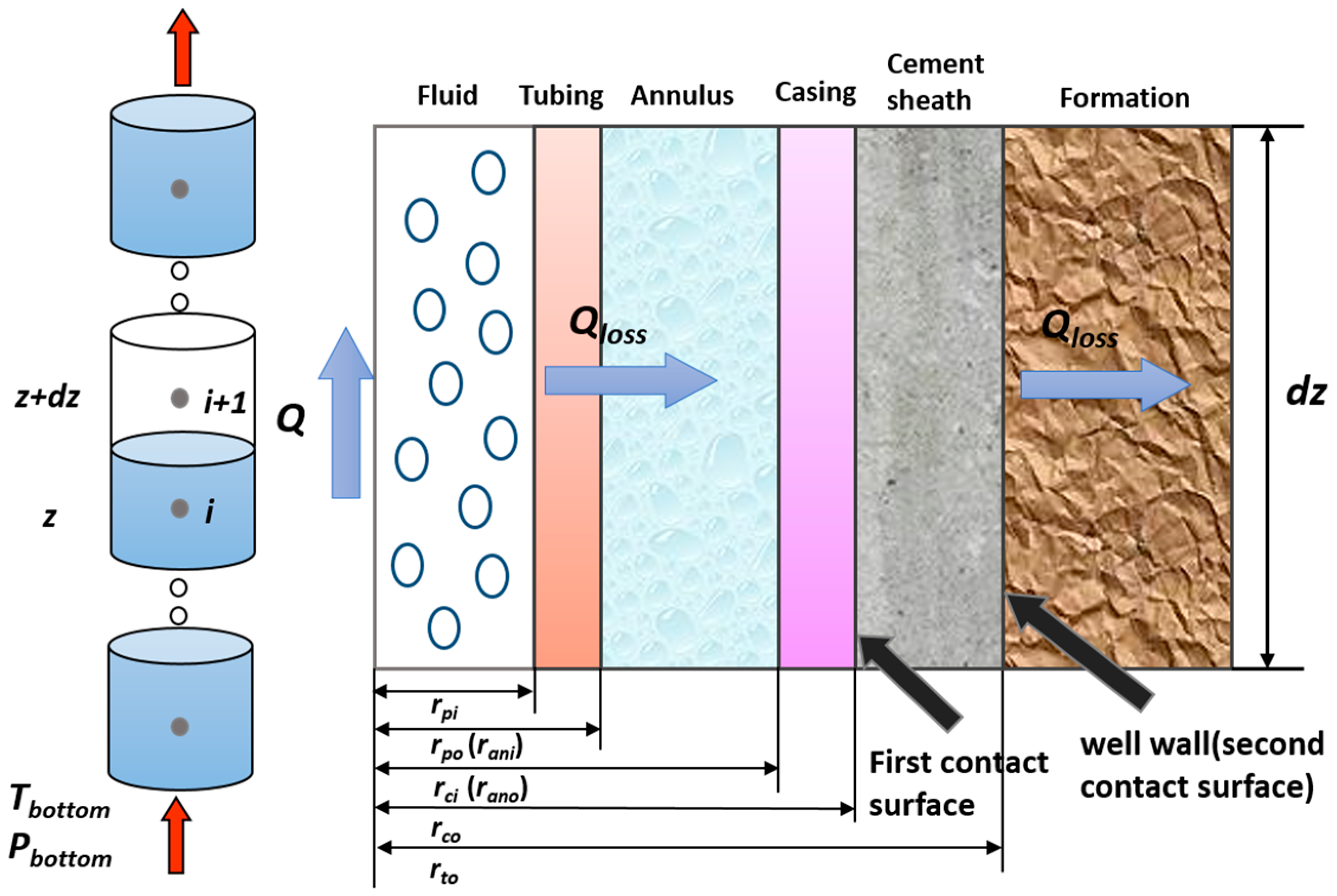
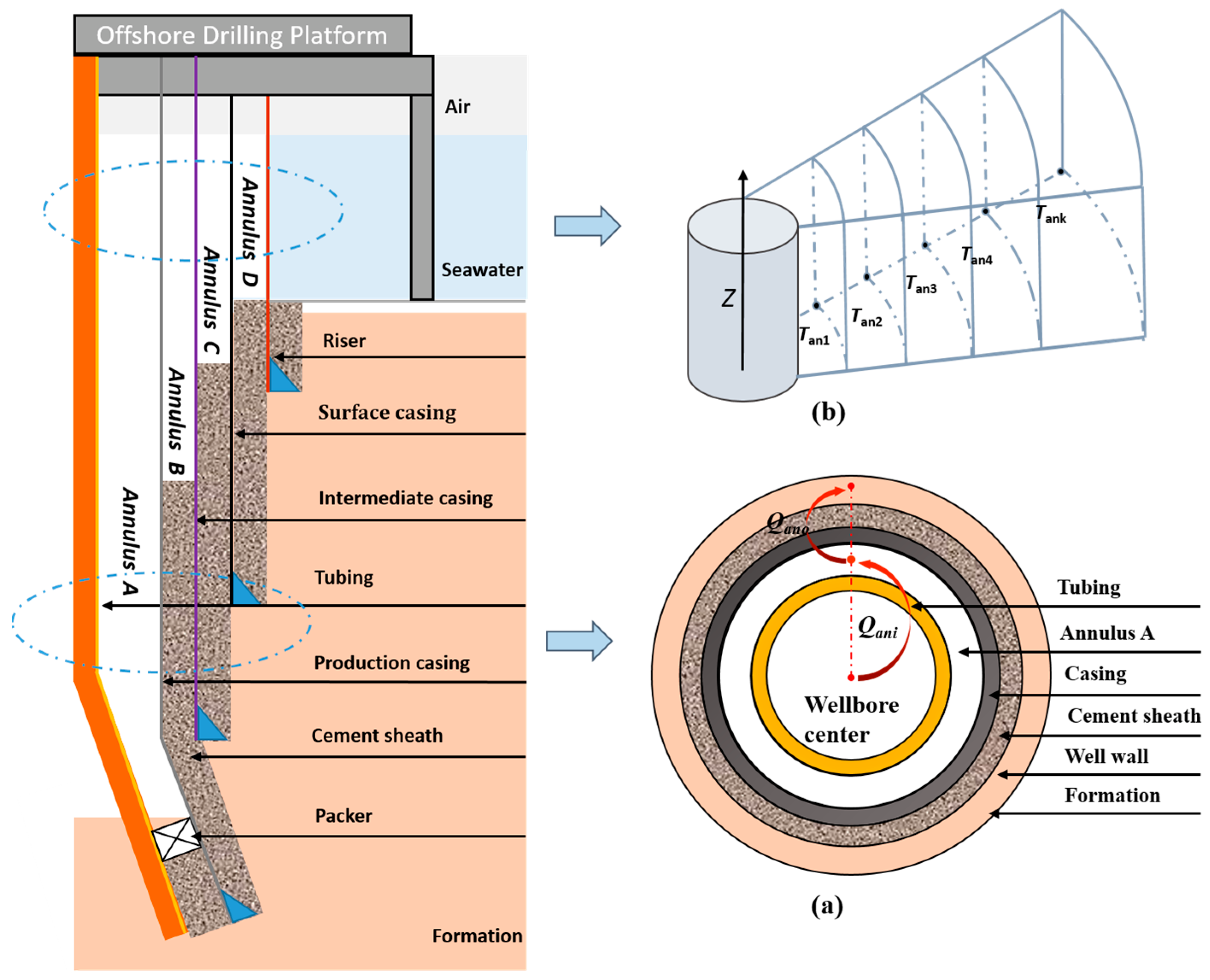
2. Calculation Model of Wellbore Temperature Field

Figure 1 shows the wellbore structure. According to different wellbore structures, regions are divided, and a heat-transfer model between the wellbore and the external environment is established. The temperature field and pressure-field coupling should be calculated first, followed by multiple annular temperatures in semi-steady mode. Due to fluid migration from the bottom-up along the tubing, fluid temperature is significantly higher than environment temperature in the same plane, resulting in heat transfer between them. Before establishing the calculation model, the following assumptions must be made:

• Assume that gas–liquid two-phase fluid flows in a one-dimensional steady direction in the tubing. The fluid flow is turbulent flow, and there is no phase change.
• Tubing is concentric with the riser, casing, formation, and cement sheath. Further, the cement sheath is well-bonded to the formation and casing.
• The temperature profile of the formation and seawater is approximately linear. Further, the air temperature is considered the same as the temperature of the sea level.
• When the fluid flows in the tubing, only the heat-transfer process occurs, and no energy exchange with the outside world occurs.
• Radial heat transfer occurs between the fluid in the tubing and the environment, and axial heat transfer in the flow direction is ignored.

2.1. Tubing Heat-Transfer Model

Figure 2 depicts wellbore heat transfer. Taking a micro-segment of the tubing for example, the arrow indicates the flow direction. According to the law of energy conservation, the energy expression of this micro-segment is obtained:

$$-Q=\Delta H+mg\cos \theta \Delta h+\frac{m\Delta v^2}{2}$$

(1)

where $H$ is the fluid of enthalpy, $\mathrm{J}$; $g$ is gravitational acceleration, $\mathrm{m}/{\mathrm{s}}^2$; $v$ is fluid velocity, $\mathrm{m}/\mathrm{s}$; and $Q$ is heat loss in a micro-segment, $\mathrm{J}$.

The differential formula can be obtained by deriving Equation (2):

$$-\frac{dq}{dz}=\frac{dh}{dz}+g\cos \theta +v\frac{dv}{dz}$$

(2)

where $q$ is the heat loss of the micro-segment in unit time, $\mathrm{J}/\left(\mathrm{m}\cdot \mathrm{s}\right)$; $h$ is the specific enthalpy of gas, $\mathrm{J}/\mathrm{k}\mathrm{g}$; and $\theta$ is the well inclination angle, $°$.

Fluid heat flowing into the tubing ($Q_{in}$) equals the sum of heat flowing out of the micro-segment per unit time ($Q_{out}$) and radial heat loss ($Q_{loss}$).

$$Q_{in}=Q_{out}+Q_{loss}$$

(3)

Fluid flows axially from bottom to wellhead, so the loss of the wellbore micro-segment in unit time—namely, heat transmitted from fluid to well wall—is [19,20]:

$$\frac{dq}{dz}=\frac{2\pi r_{po}{U}_T\left(T_f-T_{to}\right)}{\omega }$$

(4)

where $r_{po}$ is the outer diameter of the tubing, m; $U_T$ is the total heat-transfer coefficient of the wellbore, $\mathrm{J}/\left(\mathrm{s}\cdot {\mathrm{m}}^2\cdot °\mathrm{C}\right)$; $T_f$ is the fluid temperature of the tubing, $°\mathrm{C}$; $T_{to}$ is wellbore temperature, $°\mathrm{C}$; and $\omega$ is mass flow rate, kg/s.

The total thermal resistance of radial heat transfer in the wellbore is composed of the thermal resistance of fluid in tubing (R_f), string thermal resistance (R_p and R_c), annulus fluid thermal resistance (R_an), and cement sheath thermal resistance (R_cem) in a series. The specific calculation equation of the total heat transfer coefficient of the wellbore, according to the heat-transfer principle of thick wall cylinder, is [21]:

$$U_T==\frac{1}{2\pi r_{po}}{R}_T^{-1}={\left[\begin{array}{c}\frac{r_{po}}{r_{pi}{h}_f}+\frac{r_{po}\ln \left(\raisebox{1ex}{$r_{po}$}\!\left/ \!\raisebox{-1ex}{$r_{pi}$}\right.\right)}{k_p}+\frac{r_{po}\ln \left(\raisebox{1ex}{$r_{to}$}\!\left/ \!\raisebox{-1ex}{$r_{kco}$}\right.\right)}{k_{cem}}+\\ {\displaystyle \sum _{k=1}^k\frac{1}{h_{kanc}+h_{kanr}}+{\displaystyle \sum _{k=1}^k\frac{r_{po}\ln \left(\raisebox{1ex}{$r_{kco}$}\!\left/ \!\raisebox{-1ex}{$r_{kci}$}\right.\right)}{k_{ck}}}}\end{array}\right]}^{-1}$$

(5)

where $R_T$ is the total heat-transfer coefficient of the wellbore, $\mathrm{J}/\left(\mathrm{s}\cdot {\mathrm{m}}^2\cdot °\mathrm{C}\right)$; $k$ is the number of annulus in the wellbore; $h_{kanc}$ is the convective heat-transfer coefficient of the kth annulus, $\mathrm{J}/\left(\mathrm{s}\cdot {\mathrm{m}}^2\cdot °\mathrm{C}\right)$; $h_{kanr}$ is the radiative heat-transfer coefficient of the kth annulus, $\mathrm{J}/\left(\mathrm{s}\cdot {\mathrm{m}}^2\cdot °\mathrm{C}\right)$; $r_{kco}$ is the outer radius of the outer casing of the kth annulus, m; $r_{kci}$ is the inner radius of the outer casing of the kth annulus, m; and $k_{ck}$ is the thermal conductivity of the outer casing of the kth annulus, $\mathrm{J}/\left(\mathrm{s}\cdot {\mathrm{m}}^2\cdot °\mathrm{C}\right)$.

The convection heat-transfer coefficient of the production fluid is [22]:

$$\begin{array}{l}{h}_L=0.0135R{e}_L^{0.8}P{r}_L^{0.33}\left(\frac{k_L}{r_{pi}}\right){\left(\frac{{\mu }_L}{{\mu }_w}\right)}^{0.14}\\ h_{TP}=h_L{F}_p\left[1+0.55{\left(\frac{x}{1-x}\right)}^{0.1}{\left(\frac{1-F_p}{F_p}\right)}^{0.4}{\left(\frac{P{r}_g}{P{r}_L}\right)}^{0.25}{\left(\frac{{\mu }_L}{{\mu }_g}\right)}^{0.25}{I}^{0.25}\right]\end{array}$$

(6)

where $h_L$ is the liquid convection heat-transfer coefficient of the tubing, $\mathrm{J}/\left(\mathrm{s}\cdot {\mathrm{m}}^2\cdot °\mathrm{C}\right)$; $k_L$ is the thermal conductivity of the tubing liquid, $\mathrm{J}/\left(\mathrm{s}\cdot \mathrm{m}\cdot °\mathrm{C}\right)$; $R{e}_L$ is the in situ liquid-phase Reynolds number of the tubing liquid, dimensionless; $Pr$ is the Prandtl constant, dimensionless; ${\mu }_w$ is the dynamic viscosity of the production casing wall, $\mathrm{P}\mathrm{a}\cdot \mathrm{s}$; and $F_p$ is the fluidity factor, dimensionless.

The calculation formula of the in situ Reynolds number of the tubing liquid is:

$$R{e}_L=\frac{2{\omega }_L}{\pi r_{pi}{\mu }_L\sqrt{1-{\phi }_g}}$$

(7)

The calculation formula of the fluidity factor is:

$$F_p=\left(1-{\phi }_g\right)+{\phi }_g{F}_s^2$$

(8)

where ${\phi }_g$ is gas holdup, dimensionless; $F_s$ is the shape factor, dimensionless.

The shape factor calculation formula is:

$$F_s=\left[\frac{2}{\pi }\arctan \left(\sqrt{\frac{{\rho }_g{\left(v_g-v_L\right)}^2}{2g{r}_{pi}\left({\rho }_L-{\rho }_g\right)}}\right)\right]$$

(9)

The calculation formula of the inclination coefficient is:

$$I=1+\frac{4\left({\rho }_L-{\rho }_g\right)g{r}_{pi}^2}{{\sigma }_p}\left|\cos \theta \right|$$

(10)

where ${\sigma }_p$ is surface tension, $\mathrm{N}/\mathrm{m}$.

Heat transfer from well-wall to formation in a wellbore micro-segment:

$$\frac{d{q}^{\prime }}{dz}=\frac{2\pi k_d\left(T_{to}-T_d\right)}{f\left(t_D\right)}$$

(11)

where $f\left(t_d\right)$ is the dimensionless time function of formation, dimensionless; $k_d$ is the thermal conductivity of the formation, $\mathrm{J}/\left(\mathrm{s}\cdot \mathrm{m}\cdot °\mathrm{C}\right)$; and $T_d$ is the formation temperature at any depth of well, $°\mathrm{C}$.

According to the heat-transfer model and the transient heat-transfer function improved by Ramey and Hasan in the steady heat-transfer process, the dimensionless time function of the formation can be obtained as follows [23]:

$$\left\{\begin{array}{ll}{t}_D={\lambda }_d\frac{t}{r_{to}^2}& \\ f\left(t_D\right)=1.128\sqrt{t_D}\left(1-0.3\sqrt{t_D}\right)& t_D\le 1.5\\ f\left(t_D\right)=\left(0.4063+0.5ln{t}_D\right)\left(1+\frac{0.6}{t_D}\right)& t_D>1.5\end{array}\right.$$

(12)

where ${\lambda }_D$ is the thermal diffusion coefficient of the formation, ${\mathrm{m}}^2/\mathrm{s}$; $t_D$ is dimensionless time, dimensionless; and $t$ is the production time, $\mathrm{s}$.

When drilling and completing a well on an offshore platform, the seawater section of the mud line is run into a riser to isolate the seawater. Below the mudline, the wellbore temperature gradually decreases with the decrease in formation depth. Above the mud line, the wellbore temperature is affected by the seawater temperature, which drops from the sea level temperature to the temperature at the mud line (the mudline temperature is 0–4 $°\mathrm{C}$).

The heat-transfer process of the riser section wellbore is similar to the heat-transfer model below the mudline, including the heat transfer of the oil casing wall, the heat transfer between the casing wall and the riser wall, and the convective heat transfer between the riser wall and the seawater.

Heat transfer from well wall to seawater in a wellbore micro-segment:

$$\frac{d{q}^{\prime }}{dz}=2\pi r_{po}{h}_{sea}\left(T_{to}-T_{sea}\right)$$

(13)

where $h_{sea}$ is the convective heat-transfer coefficient between seawater and casing wall, $\mathrm{J}/\left(\mathrm{s}\cdot {\mathrm{m}}^2\cdot °\mathrm{C}\right)$; $T_{sea}$ is the formation temperature at any depth of well, $°\mathrm{C}$.

The convective heat-transfer coefficient of seawater:

$$h_{sea}=\frac{N{u}_{sea}{k}_{sea}}{2r_{ro}}$$

(14)

where $N{u}_{sea}$ is the Nusselt coefficient of seawater, dimensionless; $k_{sea}$ is the thermal conductivity of seawater, $\mathrm{J}/\left(\mathrm{s}\cdot \mathrm{m}\cdot °\mathrm{C}\right)$; and $r_{ro}$ is the outer diameter of the riser, $\mathrm{m}$.

The Nusselt relation of the riser under different seawater flow states is as follows [17]:

$$\begin{array}{ll}N{u}_{sea}=0.02183{\mathrm{Re}}^{0.9434}\hspace{1em}& {\mathrm{Pr}}^{1/3} \mathrm{Re}\le 2000\\ N{u}_{sea}=35.7273{\mathrm{Re}}^{0.0191}\hspace{1em}& {\mathrm{Pr}}^{1/3} 2000<\mathrm{Re}\le 10000\\ N{u}_{sea}=19.1161{\mathrm{Re}}^{0.0647}\hspace{1em}& {\mathrm{Pr}}^{0.4} 10000<\mathrm{Re}\end{array}$$

(15)

Between the sea level and the offshore platform, the convective heat transfer between the casing and the external air environment is not negligible. The heat transfer in the air section is similar to that in the seawater section, except that the external heat-transfer medium is different. Therefore, the seawater heat-transfer model is still adopted, and the convective heat-transfer coefficient of seawater can be changed into air.

Heat transfer from well wall to air in a wellbore micro-segment:

$$\frac{d{q}^{\prime }}{dz}=2\pi r_{po}{h}_{air}\left(T_{to}-T_{air}\right)$$

(16)

where $h_{air}$ is the convective heat-transfer coefficient between air and casing wall, $\mathrm{J}/\left(\mathrm{s}\cdot {\mathrm{m}}^2\cdot °\mathrm{C}\right)$; $T_{air}$ is the air temperature, $°\mathrm{C}$.

The air convective heat-transfer coefficient:

$$h_{air}=\frac{N{u}_{air}{k}_{air}}{2r_{ro}}$$

(17)

where $N{u}_{air}$ is the Nusselt coefficient of the air, dimensionless; $k_{air}$ is the thermal conductivity of air, $\mathrm{J}/\left(\mathrm{s}\cdot \mathrm{m}\cdot °\mathrm{C}\right)$.

The Nusselt relation of the riser under different air-flow states is as follows [24]:

$$\begin{array}{l}\mathrm{Laminar} \mathrm{flow}:\\ N{u}_{air}=1+0.3\left[{32}^{0.5}{\left(G{r}_h\right)}^{-0.25}{\left(\frac{h}{d}\right)}^{0.909}\right]{ 10}^4\le R{a}_h\le 4\times {10}^9\\ \mathrm{Transitional} \mathrm{flow}:\hspace{1em}1.08\times {10}^4\le G{r}_d\le 6.9\times 10\\ N{u}_{air}=2.9G{r}_d^{1/12}{\left(G{r}_{h}Pr\right)}^{1/4}\hspace{1em}9.88\times {10}^7\le R{a}_h\le 2.7\times {10}^9\\ N{u}_{air}=0.47G{r}_d^{-1/12}{\left(G{r}_{h}Pr\right)}^{1/4}\hspace{1em}2.7\times {10}^9<R{a}_h<2.95\times {10}^{10}\\ \mathrm{Turbulence}:\\ N{u}_{air}=0.13R{a}_h^{1/3}\\ N{u}_{air}=0.582\times {10}^{-5}R{a}_h^{0.675}\hspace{1em}70\le h/d\le 136\end{array}$$

(18)

where:

$$\begin{array}{l}G{r}_d=\frac{g{\alpha }_{air}\Delta T_r{d}^3}{{\gamma }_{air}^2}\\ G{r}_h=\frac{g{\alpha }_{air}\Delta T_r{h}^3}{{\gamma }_{air}^2}\\ R{a}_h=G{r}_{h}Pr\left(P{r}_{air}=0.71\right)\end{array}$$

(19)

where $R{a}_h$ is the Rayleigh number of the air, dimensionless.

Radial heat in and out of the micro-segment per unit time can be considered equal for the second contact surface.

$$\frac{d{q}^{\prime }}{dz}=\frac{dq}{dz}$$

(20)

Combined with Equations (4), (12), (13), (16) and (20), the well wall temperature in different heat-transfer environments is:

$$\begin{array}{ll}\mathrm{Formation}:& T_{\mathrm{to}}=\frac{f\left(t_D\right)r_{po}{U}_T{T}_f+k_d{T}_d}{f\left(t_D\right)r_{po}{U}_T+k_d}\\ \mathrm{Seawater}:& T_{\mathrm{to}}=\frac{U_T{T}_f+h_{air}\omega T_{air}}{U_T+h_{air}\omega }\\ \mathrm{Air}:& T_{\mathrm{to}}=\frac{U_T{T}_f+h_{sea}\omega T_{sea}}{U_T+h_{sea}\omega }\end{array}$$

(21)

The relationship between specific enthalpy and temperature and pressure is obtained from a specific heat capacity at a constant pressure and the Joule–Thomson coefficient, according to the first law of thermodynamics:

$$\frac{dh}{dz}=-C_J{C}_P\frac{d{P}_f}{dz}+C_p\frac{d{T}_f}{dz}$$

(22)

where $C_J$ is the Joule–Thomson coefficient, $\mathrm{K}/\mathrm{P}\mathrm{a}$; $C_p$ is the specific heat capacity of the fluid at constant pressure, $\mathrm{J}/\left(\mathrm{k}\mathrm{g}\cdot \mathrm{K}\right)$.

The pressure gradient formula of gas–liquid two-phase flow is:

$$\frac{dp}{dz}=-{\rho }_f\mathrm{gcos}\theta -f\frac{{\rho }_f{v}_f{}^2}{4r_{pi}}-{\rho }_f{v}_f\frac{d{v}_f}{dz}$$

(23)

where ${\rho }_f$ is the mixed fluid density, $\mathrm{k}\mathrm{g}/{\mathrm{m}}^3$; $f$ is the friction coefficient, dimensionless; and $r_{pi}$ is the tubing radius, $\mathrm{m}$.

The gas-phase flow rate in the tubing is:

$$\begin{array}{l}{v}_g=B_f{v}_{st}=1.27\times {10}^{-9}\frac{Q_{st}Z{T}_f}{r_{pi}^2{P}_f}\\ B_f=3.447\times {10}^{-4}\frac{Z{T}_f}{P_f}\end{array}$$

(24)

where $B_f$ is the volume coefficient of natural gas, $\mathrm{K}/\mathrm{M}\mathrm{P}\mathrm{a}$; $v_{st}$ is the gas-phase flow rate under standard state, $\mathrm{m}/\mathrm{s}$; Z is the deviation factor of natural gas, dimensionless; $P_f$ is the pressure of the fluid acting on the tubing, $\mathrm{M}\mathrm{P}\mathrm{a}$; and $Q_{st}$ is the gas flow under standard state, ${\mathrm{m}}^3/\mathrm{d}$.

The liquid-phase flow rate in the tubing is:

$$v_l=\frac{Q_l}{86400\pi r_{pi}^2}$$

(25)

where $v_l$ is the liquid flow rate, $\mathrm{m}/\mathrm{s}$; $Q_l$ is the liquid flow of the tubing, ${\mathrm{m}}^3/\mathrm{d}$.

The actual velocity of gas–liquid two-phase is [25]:

$$v_f=v_g+v_l$$

(26)

The gas density in the tubing is:

$${\rho }_g=\frac{P_f{M}_f}{ZR{T}_f}=3484.28\frac{P_f{S}_g}{Z{T}_f}$$

(27)

where $s_g$ is the gas relative density of the tubing.

By the volume-weighted calculation of gas–liquid two-phase density, the mixed fluid density in the tubing is:

$${\rho }_f={\rho }_g{\phi }_g+{\rho }_l(1-{\phi }_g)$$

(28)

where ${\rho }_l$ is the liquid density of the tubing, $\mathrm{k}\mathrm{g}/{\mathrm{m}}^3$.

Liquid holdup reflects the ratio of liquid to production fluid on the section of tubing. The calculation formula is:

$${\phi }_g=\frac{v_g}{C_o{v}_f+v_{gm}}$$

(29)

where $C_o$ is a distribution parameter, dimensionless; $v_{gm}$ is the drift speed, $\mathrm{m}/\mathrm{s}$.

The calculation formula of the distribution parameters is:

$$C_o=\lambda \left[1+{\left(\frac{v_L}{v_g}\right)}^{{\left({\rho }_g/{\rho }_L\right)}^{0.1}}\right]$$

(30)

The calculation formula of drift speed is [22]:

$$v_{gm}=2.9{\left[\frac{2g{r}_{pi}{\sigma }_p\left(1+\cos \theta \right)\left({\rho }_L-{\rho }_g\right)}{{\rho }_L^2}\right]}^{0.25}{\left(1.22+1.22\sin \theta \right)}^{p_{atm}/p_{sys}}$$

(31)

The calculation formula of gas volume flow fraction $\lambda$ is:

$$\lambda =\frac{v_g}{v_g+v_L}$$

(32)

Bring Equations (4), (21) and (23) into Equation (2) to obtain:

$$\beta \left(T_f-T_d\right)=C_p\frac{d{T}_f}{dz}+g\cos \theta -C_p{C}_J\frac{d{P}_f}{dz}+v_f\frac{d{v}_f}{dz}$$

(33)

Fluid temperature at the outlet of a micro-segment in formation is obtained by solving the first-order differential Equation (33):

$$\begin{array}{l}{T}_{fo}=T_{do}+e^{-\Delta z\beta /C_p}\left(T_{fi}-T_{di}\right)+\frac{1}{\beta }\left(1-e^{-\Delta z\beta /C_p}\right)\\ \hspace{1em}\left(C_p{C}_J\frac{P_{fo}-P_{fi}}{\Delta z}-v_f\frac{v_{fo}-v_{fi}}{\Delta z}-g\cos \theta +C_p{G}_h\cos \theta \right)\\ \beta =\frac{2\pi r_{po}{U}_T}{\omega \left(r_{po}{U}_{T}f\left(t_D\right)+k_d\right)}\end{array}$$

(34)

Fluid temperature at the outlet of a micro-segment in seawater is obtained using the same solution process:

$$\begin{array}{l}{T}_{fo}=T_{seao}+e^{-\Delta z\beta /C_p}\left(T_{fi}-T_{di}\right)+\frac{1}{\beta }\left(1-e^{-\Delta z\beta /C_p}\right)\\ \hspace{1em}\left(C_p{C}_J\frac{P_{fo}-P_{fi}}{\Delta z}-v_f\frac{v_{fo}-v_{fi}}{\Delta z}-g\cos \theta +C_p{G}_h\cos \theta \right)\\ \beta =\frac{2\pi r_{po}{U}_T{h}_{sea}}{\omega \left(U_T+h_{sea}\right)}\end{array}$$

(35)

Similarly, fluid temperature at the outlet of a micro-segment in seawater is obtained by:

$$\begin{array}{l}{T}_{fo}=T_{airo}+e^{-\Delta z\beta /C_p}\left(T_{fi}-T_{airi}\right)+\frac{1}{\beta }\left(1-e^{-\Delta z\beta /C_p}\right)\\ \hspace{1em}\left(C_p{C}_J\frac{P_{fo}-P_{fi}}{\Delta z}-v_f\frac{v_{fo}-v_{fi}}{\Delta z}-g\cos \theta \right)\\ \beta =\frac{2\pi r_{po}{U}_T{h}_{air}}{\omega \left(U_T+h_{air}\right)}\end{array}$$

(36)

The wellbore is divided into countless micro-segments, and the outlet temperature of each micro-segment is calculated as the inlet temperature of the next section, which is successively calculated until the wellhead fluid temperature is obtained, and finally, the tubing temperature profile is obtained.

2.2. Wellbore Annulus Temperature Calculation

Figure 3a illustrates the single-layer annulus heat transfer. The heat flowing into the annulus $Q_{ano}$ is equal to the heat flowing out of the annulus per unit of time. Further, the single-layer annulus temperature can be calculated by [26]:

$$T_{an1}=\frac{2\pi T_f{U}_f{r}_{po}+\beta \omega {\mathrm{T}}_d}{2\pi U_f{r}_{po}+\beta \omega }$$

(37)

where:

$$\begin{array}{l}{U}_f=\frac{r_{po}}{r_{pi}{h}_f}+\frac{r_{po}\ln \left(\raisebox{1ex}{$r_{po}$}\!\left/ \!\raisebox{-1ex}{$r_{pi}$}\right.\right)}{k_p}\\ \end{array}$$

(38)

Figure 3b depicts the progress of dividing each annulus into a radial mesh. Establish a coordinate system, and the direction of fluid flow is the positive direction of the z-axis. According to Fourier’s law of thermal conductivity, calculate the annulus temperature. Then, the heat transfer of the kth annulus can be expressed as:

$$2\pi k_{an}{r}_{ank}{h}_{anck}\frac{T_{ank-1}^{n+1}-T_{ank}^{n+1}}{\Delta r_{ank}}+2\pi k_{an}{r}_{ank+1}{h}_{anck+1}\frac{T_{ank}^{n+1}-T_{ank+1}^{n+1}}{\Delta r_{ank+1}}=C_{pan}{\rho }_{an}\pi \Delta r_{ank}^2{h}_{anck}\frac{T_{ank}^{n+1}-T_{ank}^n}{\Delta t}$$

(39)

Where $k_{an}$ is thermal conductivity of fluid in the annulus, $\mathrm{J}/\left(\mathrm{s}\cdot \mathrm{m}\cdot °\mathrm{C}\right)$; $\Delta r_{ank}$ is the difference between the outer surface radius of the kth annulus and the outer surface radius of the (k + 1)th annulus, m.

3. Wellbore Pressure Field Calculation Model

In the process of offshore HPHT gas-well exploitation, a small amount of liquid phase such as water and oil and natural gas are extracted to the wellhead at the same time, so the calculation model of separated flow pressure drop can be adopted. Different from the homogeneous flow model, it considers the slip at the gas–liquid interface.

The pressure drop of a flow pipeline mainly consists of three parts: hydrostatic pressure drop caused by the axial flow of pipeline fluid, pressure drop caused by friction of the pipe wall and gas–liquid interface, and pressure drop caused by acceleration. The contribution of each of these sections to the total pressure drop depends on the flow mode, fluid characteristics, pipe orientation, and pipe diameter.

The hydrostatic pressure drop of gas–liquid two-phase flow is [27]:

$${\left(\frac{dP}{dz}\right)}_h={\rho }_{m}g\sin \theta$$

(40)

The pressure drop caused by the acceleration of gas–liquid two-phase flow is:

$${\left(\frac{dP}{dz}\right)}_a={\rho }_m^2{v}_f^2\frac{d}{dz}\left(\frac{x^2}{{\phi }_g{\rho }_g}+\frac{{\left(1-E\right)}^2{\left(1-x\right)}^2}{\beta {\rho }_l}+\frac{E^2{\left(1-x\right)}^2}{\left(1-{\phi }_g-\beta \right){\rho }_l}\right)$$

(41)

$\beta$ is the correction coefficient of gas holdup, and the calculation formula is:

$$\beta =1-{\phi }_g-\frac{{\phi }_{g}E\left(1-x\right){\rho }_g}{x{\rho }_l}$$

(42)

$E$ is the liquid entrainment fraction. Due to the relative motion between the gas and liquid phases, a special phenomenon called entrainment can be observed. The entrainment process is characterized by tiny droplets flowing into a rapidly moving gas phase at the center. Liquid entrainment is due to the obvious shear phenomenon at the gas–liquid interface, which depends on the fluid flow rate, pipe diameter and direction, and the surface tension at the gas–liquid interface. The liquid entrainment fraction $E$ is defined as the ratio of the mass flow rate of droplets entering the gas phase to the total mass flow rate of the liquid phase.

The calculation formula of liquid entrainment fraction is:

$$\frac{E}{1-E}=0.003W{e}_c^{1.8}{\left(\frac{v_g}{\sqrt{gd}}\right)}^{-0.92}R{e}_g^{-1.24}{\left(\frac{{\rho }_L}{{\rho }_c}\right)}^{0.38}{\left(\frac{{\mu }_L}{{\mu }_g}\right)}^{0.9}$$

(43)

where $W{e}_c$ is the Weber number, dimensionless; ${\rho }_c$ is the fluid core density, $\mathrm{k}\mathrm{g}/{\mathrm{m}}^3$.

The calculation formula of the Weber number is:

$$W{e}_c=\frac{\rho v_g^{2}d}{{\sigma }_P}$$

(44)

The fluid core density calculation formula is:

$${\rho }_c={\rho }_g\left[1+E\left(\frac{v_L}{v_g}\right)\left(\frac{{\rho }_L}{{\rho }_g}\right)\right]$$

(45)

In this paper, the friction pressure drop is calculated by selecting two-phase frictional multiplier ${\mathrm{\Phi }}_{lo}^2$, which is summarized by Ghajar and Bhagwat through a large number of experiments. The pressure drop caused by interface friction for gas–liquid two-phase flow is:

$$\begin{array}{l}{\left(\frac{dP}{dz}\right)}_f={\mathrm{\Phi }}_{LO}^2{\left(\frac{dP}{dz}\right)}_{LO}\\ {\left(\frac{dP}{dz}\right)}_{LO}=\frac{f_l{\rho }_m^2{v}_f^2}{r_{pi}{\rho }_l}\end{array}$$

(46)

The calculation formula of two-phase frictional multiplier ${\mathrm{\Phi }}_{lo}^2$ is:

$${\mathrm{\Phi }}_{lo}^2=\left\{{\left(1-x\right)}^{0.33}\left[1+B_{1}x\left(Y^2-1\right)\right]+B_2{Y}^2{x}^3\right\}\left(1+B_3{\left(1-x\right)}^2\right)$$

(47)

where $B_1$, $B_2$, $B_3$, ${\mathrm{\Pi }}_1$, ${\mathrm{\Pi }}_2$, ${\mathrm{\Pi }}_3$, $\zeta$, Bo, and Y are the calculation parameters and correction coefficient of two-phase frictional multiplier ${\mathrm{\Phi }}_{lo}^2$(for the specific formula, please refer to the literature [21,25]).

For laminar flow and turbulent flow in a circular pipe, this calculation method can be used to calculate the friction coefficient of single-phase string [28]:

$$f=2{\left[{\left(\frac{8}{\mathrm{Re}}\right)}^{12}+\frac{1}{{\left(a+b\right)}^{1.5}}\right]}^{\raisebox{1ex}{$1$}\!\left/ \!\raisebox{-1ex}{$12$}\right.}$$

(48)

where:

$$\begin{array}{l}a={\left\{2.457\ln \left[\frac{1}{{\left(7/\mathrm{Re}\right)}^{0.9}+\left(0.135e/r_{pi}\right)}\right]\right\}}^{16}\\ b={\left(\frac{37530}{\mathrm{Re}}\right)}^{16}\end{array}$$

(49)

where $e$ is the absolute roughness of the tubing wall, $\mathrm{m}$.

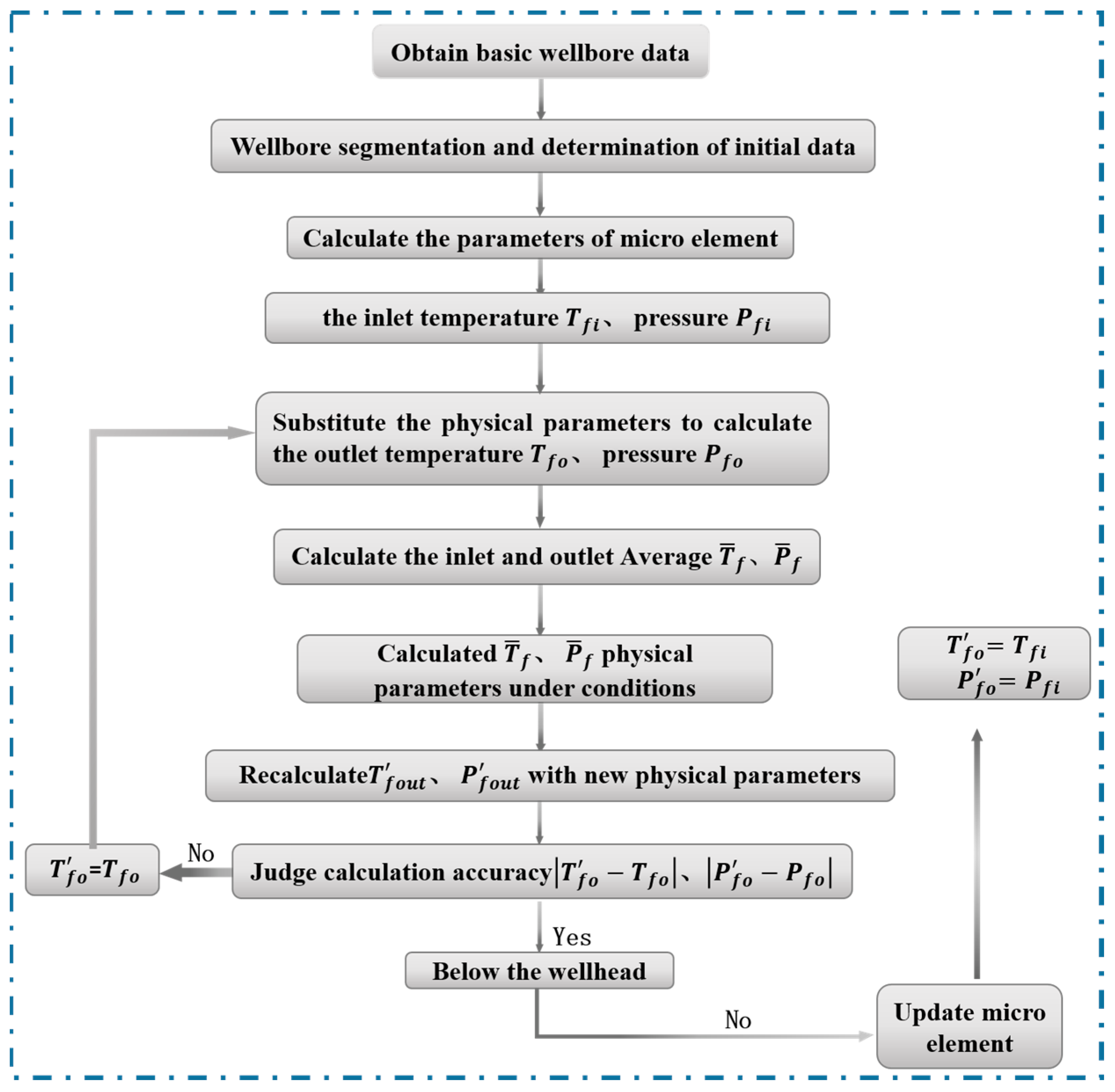
4. Example Calculation

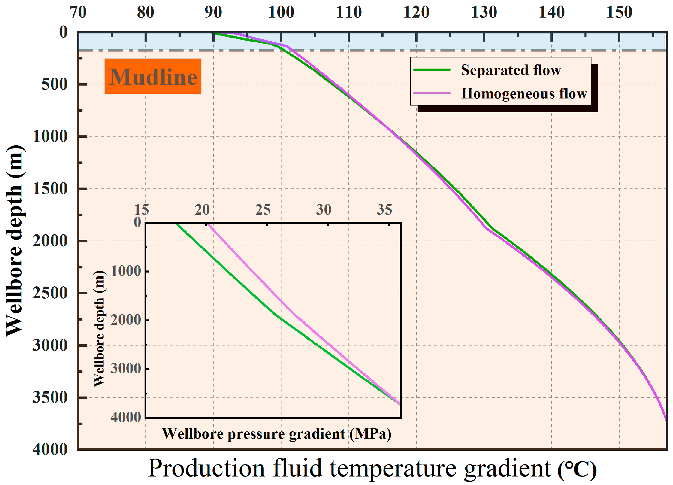
4.1. Model Verification

In order to ensure the reliability of the results of the calculation model established in this paper, a gas well in the China sea is used for an example. This case well is a directional well. The basic parameters are shown in

Table 1. Basic parameters of case well.

Parameter	Value	Parameter	Value
Formation temperature	$157 °\mathrm{C}$	Cement sheath thermal conductivity	$0.958 \mathrm{J}/\left(\mathrm{s}\cdot \mathrm{m}\cdot °\mathrm{C}\right)$
Formation pressure	36 MPa	Formation thermal conductivity	$1.73 \mathrm{J}/\left(\mathrm{s}\cdot \mathrm{m}\cdot °\mathrm{C}\right)$
Mudline temperature	$0.0428 °\mathrm{C}/\mathrm{m}$	Annulus liquid thermal conductivity	$0.66 \mathrm{J}/\left(\mathrm{s}\cdot \mathrm{m}\cdot °\mathrm{C}\right)$
Seawater temperature gradient	$0.195 °\mathrm{C}/\mathrm{m}$	Annulus liquid density	$1250 \mathrm{kg}/{\mathrm{m}}^3$
Air temperature	$26 °\mathrm{C}$	Annulus liquid specific heat capacity	$4050 \mathrm{J}/\left(\mathrm{kg}\cdot °\mathrm{C}\right)$
Formation thermal diffusivity	$1.17\times {10}^{-6} {\mathrm{m}}^2/\mathrm{s}$	Annulus fluid viscosity	$0.051 \mathrm{mPa}\cdot \mathrm{s}$
Gas production	$31.5\times {10}^4 {\mathrm{m}}^3/\mathrm{d}$	Tubing thermal conductivity	$43 \mathrm{J}/\left(\mathrm{s}\cdot \mathrm{m}\cdot °\mathrm{C}\right)$
Water production	$30 {\mathrm{m}}^3/\mathrm{d}$	Casing thermal conductivity	$48 \mathrm{J}/\left(\mathrm{s}\cdot \mathrm{m}\cdot °\mathrm{C}\right)$
Oil production	$140 {\mathrm{m}}^3/\mathrm{d}$	Well inclination angle	$58.78°$
Production time	84 h	Seawater depth	120 m

and Figure 1, and the numerical calculation process is shown in Figure 4.

Figure 5 shows the comparison of the wellbore temperature and pressure field results of the case wells, which were obtained by different calculation methods. It can be seen from the figure that the results obtained by the two calculation methods are relatively close, and the variation of the wellbore temperature and pressure curve is the same. However, the wellbore data obtained by the homogeneous flow calculation are larger than that of the separated flow calculation. The wellhead temperature and pressure are selected to compare with the measured data, as shown in Figure 6. The comparison between the calculated results of homogeneous flow and the measured data shows that there is an error of 2.33% in the wellhead temperature and an error of 17.45% in the wellhead pressure. Compared with the measured data, the calculated results of the separated flow in this paper show an error of 0.87% in wellhead temperature and only 2.46% in wellhead pressure. This shows that the calculation model established in this paper has higher accuracy and is more consistent with the measured data, which greatly improves the accuracy of wellbore temperature and pressure.

4.2. Wellbore Temperature Field

Figure 7 shows the wellbore temperature curve obtained by using the calculation model in this paper. We can see from the drawings: (1) in the formation section, the fluid temperature in the tubing decreases slowly with the decrease in well depth; (2) in the seawater–air section, forced convection heat exchange between seawater–air and wellbore is stronger than that between wellbore and formation. Further, production fluid temperature decreases significantly faster. The annulus temperature of the formation section declines gradually with depth decreases. However, there is a sharp change near the mudline, and the annulus temperature drops rapidly. After entering the seawater section completely, the temperature of each annulus gradually decreases with the decrease in seawater depth, and the temperatures between annulus temperatures are close to each other. The maximum temperature difference is only about 7 $°\mathrm{C}$. As a result, the impact of the seawater section and air section on wellbore temperature cannot be ignored for offshore wells.

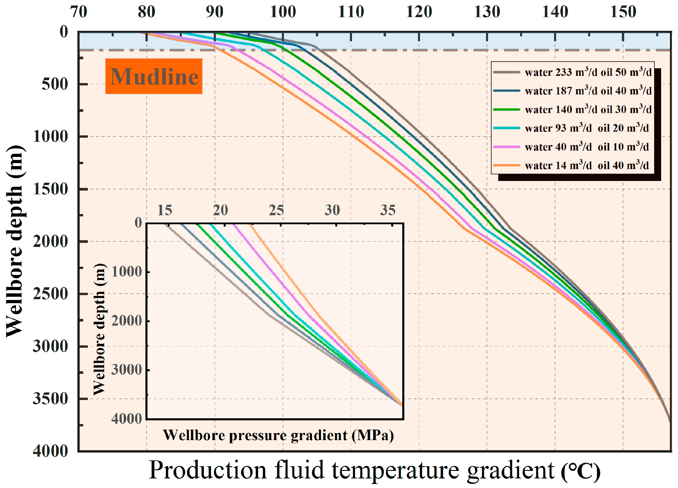
4.3. Gas–Liquid Ratio Production Fluid

Figure 8 depicts the influence of gas–liquid ratio on wellbore temperature and pressure under the conditions of gas production of $31.5 \times {10}^4\cdot {\mathrm{m}}^3/\mathrm{d}$, production time of 84 h, and the same oil–water ratio of production fluid (14:3). As can be seen from the figure, since the specific heat capacity of liquid phase is much larger than that of gas phase, the wellbore temperature becomes increasingly high with the increase in liquid oil–water content in the mixed fluid. However, the increase in liquid content will increase the density of gas–liquid mixture, which makes hydrostatic pressure drop and friction pressure drop increase. As a result, the wellbore pressure drop decreases continuously, showing a trend of wellbore pressure decreasing with the decrease in the gas–liquid ratio (the increase in liquid content). It can also be seen from Equation (33) that wellbore temperature and pressure change in opposite trends. Therefore, by controlling the gas–liquid ratio reasonably, the wellbore pressure can be adjusted without changing the production process, so as to avoid the risk of increasing casing failure due to the high wellbore pressure.

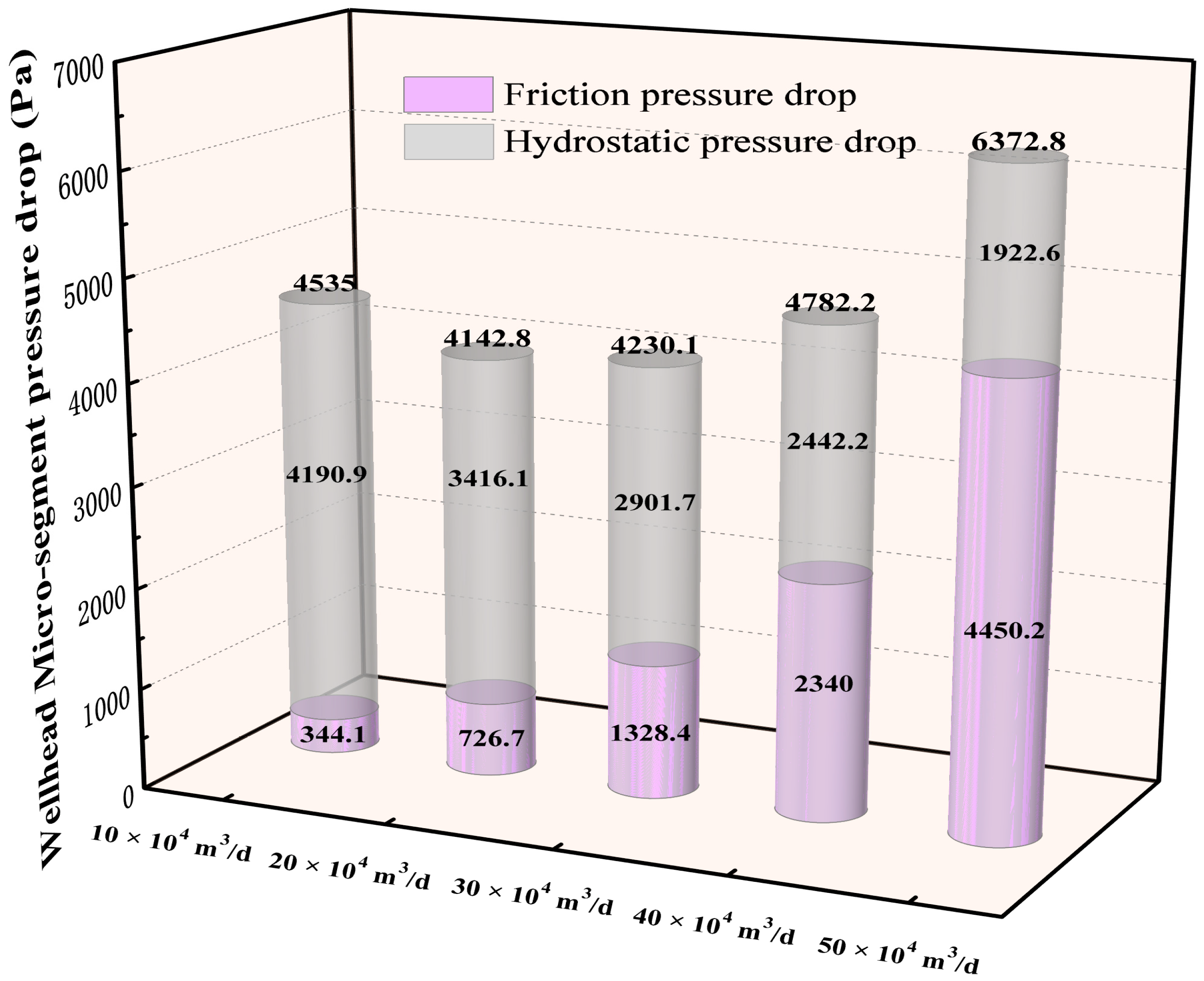
4.4. Production Conditions

Figure 9 shows the influence of gas production on wellbore temperature and pressure. Only gas production is changed, and other conditions are consistent with the case well. As can be seen from the figure, the gas production has a significant impact on the wellbore temperature. When the gas production rises from 10 $\times {10}^4\cdot {\mathrm{m}}^3/\mathrm{d}$ to 60 $\times {10}^4\cdot {\mathrm{m}}^3/\mathrm{d}$, the wellhead temperature rises from 63 $°\mathrm{C}$ to 99 $°\mathrm{C}$, which is increased by 1.6 times. However, the wellbore pressure increases first and then decreases with the increase in production because of the mutual influence of friction pressure drop and hydrostatic pressure drop. Figure 10 depicts the pressure drop in the micro-segment of the wellhead. Since the accelerated pressure drop is very small, only the friction pressure drop and hydrostatic pressure drop are shown. As can be seen from the figure, when the gas production is small, the liquid phase in the wellbore occupies a relatively high proportion, and the mixed fluid density is relatively large, resulting in a rapid hydrostatic pressure drop, and it accounts for a large proportion of the total pressure drop. However, with the increase in gas production, the fluid mixing density decreases, and the hydrostatic pressure drop slows down. At the same time, the friction at the gas–liquid interface gradually increases with the increase in the gas phase, leading to a significant decrease in the wellbore friction pressure drop, and the final wellbore pressure increases first and then decreases.

Figure 11 shows the influence of production time on wellbore temperature and pressure under the production conditions of the case well. It can be seen from the figure that the wellhead temperature increased from 91.6 $°\mathrm{C}$ to 96.4 $°\mathrm{C}$ during the period of 10 d to 100 d, while the wellhead temperature only increased by 1.8 $°\mathrm{C}$ during the period of 101 d to 300 d. This indicates that wellbore temperature tends to be stable with the increase in production time. The wellbore pressure does not change with the increase in production time in the 10~300 d production range.

Figure 12 compares the variation trend of the wellhead temperature changing with the production time that was obtained by the homogeneous method model and the separated method. As can be seen from the figure, it takes 28 days for the wellhead temperature to reach 95 $°\mathrm{C}$ in the model based on homogeneous phase flow, which is much faster than 48 days in the separated model. Therefore, the improved model can provide a more accurate estimate of the time taken to reach the rated wellhead temperature and accurate theoretical support for the rational formulation of the production plan after the well opening, so as to avoid excessive restrictions on the initial production rate.

5. Conclusions

Based on the gas–liquid two-phase separated method, an improved calculation model of wellbore temperature and pressure for gas–liquid two-phase flow in offshore gas wells is established in this paper. Further, the influencing factors of wellbore temperature and pressure are analyzed. The following conclusions are obtained:

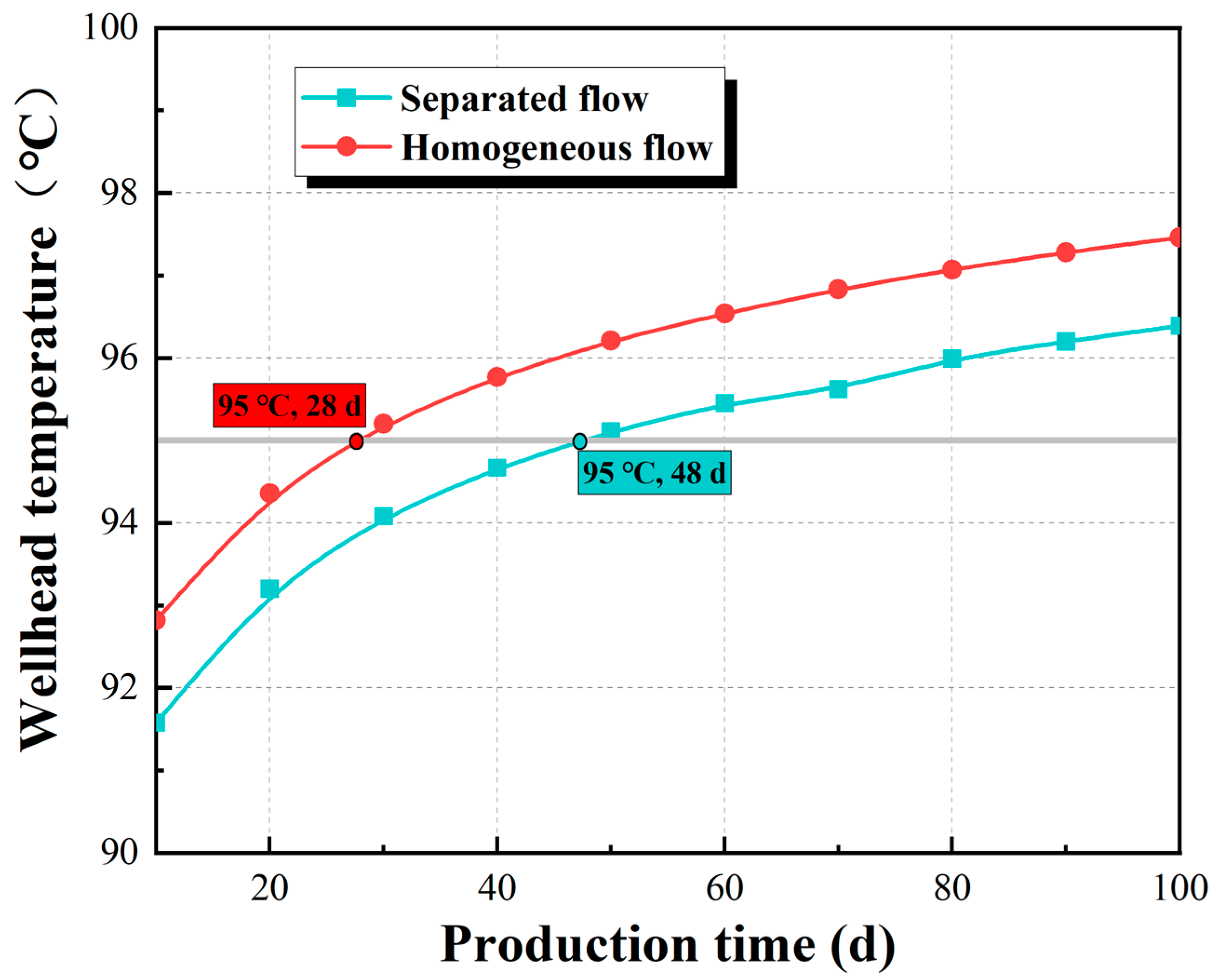
• Although the results of homogeneous flow and separated phase flow have the same trend, the errors of wellhead temperature and pressure obtained by homogeneous flow calculation are large compared with measured data, which are 2.33% and 17.45%. However, the errors of the improved model are only 0.87% and 2.46%, which greatly improves the accuracy of wellbore temperature and pressure calculation.
• Forced convection heat exchange between seawater–air and wellbore is stronger than that between wellbore and formation. As a result, the temperature drop rate of the tubing in the seawater and air sections is significantly accelerated. Therefore, the influence of the seawater and air sections on the wellbore temperature of offshore gas wells should be fully considered.
• Since the specific heat capacity of liquid phase is much larger than that of gas phase, the wellbore temperature becomes increasingly high as the gas–liquid ratio of the product decreases (liquid-phase content increases). However, it also leads to the increase in hydrostatic pressure and friction pressure loss as the mixed fluid density rises, causing the wellbore pressure decrease. Based on this trend, the liquid content of the product should be controlled in a reasonable range in order to avoid the risk of casing failure due to high wellbore pressure.
• Gas production is the key factor affecting wellbore temperature. When the gas production rises from 10 $\times {10}^4\cdot {\mathrm{m}}^3/\mathrm{d}$ to 60 $\times {10}^4\cdot {\mathrm{m}}^3/\mathrm{d}$, the wellhead temperature rises from 63 $°\mathrm{C}$ to 99 $°\mathrm{C}$. However, due to the mutual influence of friction pressure drop and hydrostatic pressure drop, wellbore pressure increases first and then decreases with the increase in gas production. It takes 28 days for the wellhead temperature to reach 95 $°\mathrm{C}$ in the model based on homogeneous-phase flow, which is much faster than 48 days in the separated model. Therefore, the improved model can provide a more accurate estimate of the time to reach the rated wellhead temperature and accurate theoretical support for the rational formulation of the production plan after the well opening, so as to avoid excessive restrictions on the initial production rate.

References

1. Luo, M.; Zhu, H.Y.; Liu, Q.Y.; Wang, Z.W.; Li, Y.J.; Han, C.; Zhang, C. A V-cutter PDC bit suitable for ultra-HTHP plastic mudstones. Nat. Gas Ind. 2021, 41, 97–106. [Google Scholar]
2. Xu, M.G.; Fan, C.W.; Zhang, D.N.; Hu, G.W.; Tan, J.C. Formation condition and hydrocarbon accumulation model in Ledong 01 Gas Reservoir of super high temperature and high pressure in the Yinggehai Basin. Nat. Gas Ind. 2021, 41, 43–53. [Google Scholar]
3. Chen, H.; Yang, C.; Datta-Gupta, A.; Zhang, J.; Chen, L.; Liu, L.; Chen, B.; Cui, X.; Shi, F.; Bahar, A. Fracture inference and optimal well placement using a multiscale history matching in a HPHT tight gas reservoir, Tarim Basin, China. Upstream Oil Gas Technol. 2020, 2, 100002. [Google Scholar] [CrossRef]
4. Wang, Y.H.; Hao, Y.Z.; Li, F.; Lu, F.F.; Deng, K.H.; Lin, Y.H. Failure mechanism of wellbore integrity for HTHP gas wells, Shunnan block, Tarim Basin. Nat. Gas Explor. Dev. 2019, 42, 86–89. [Google Scholar]
5. Xie, H.; Zhang, G.W.; Liu, X.Q.; Chen, G.M.; Chang, Y.J. Mechanism of Christmas tree rise in offshore oil and gas wells and the related calculation method. Nat. Gas Ind. 2013, 33, 80–84. [Google Scholar]
6. Ramey, H.J. Wellbore Heat Transmission. J. Pet. Technol. 1962, 4, 427–435. [Google Scholar] [CrossRef]
7. Shiu, K.C.; Begges, H. Predicting Temperatures in Flowing Oil Wells. J. Energy Resour. Technol. 1980, 102, 2–11. [Google Scholar] [CrossRef]
8. Hasan, A.R.; Kabir, C.S. Heat transfer during two phase flow in wellbores. In Proceedings of the 66th Annual Technical Conference and ExhiMion of the Society of Petroleum Engineers, Dallas, TX, USA, 6–9 October 1991. [Google Scholar]
9. Spindler, R. Analytical Models for Wellbore-Temperature Distribution. SPE J. 2011, 1, 125–133. [Google Scholar] [CrossRef]
10. Wu, Z.; Xu, J.; Wang, X.; Chen, K.; Li, X.; Zhao, X. Predicting Temperature and Pressure in High-Temperature–High-Pressure Gas Wells. Petrol. Sci. Technol. 2011, 29, 132–148. [Google Scholar] [CrossRef]
11. Xu, J.; Hu, J.; Wu, Z.; Wang, S.; Qi, B. Prediction of Temperature and Pressure Distribution in HTHP Injection Gas Wells with Thermal Effect of Wellbore. Petrol. Sci. Technol. 2013, 31, 1423–1438. [Google Scholar] [CrossRef]
12. Martínez-Cuenca, R.; Mondragón, R.; Hernández, L.; Segarra, C.; Jarque, J.C.; Hibiki, T.; Juliá, J.E. Forced-convective heat-transfer coefficient and pressure drop of water-based nanofluids in a horizontal pipe. Appl. Therm. Eng. 2016, 98, 841–849. [Google Scholar] [CrossRef]
13. Yin, B.; Li, X.; Qi, M. Study of Fluid Phase Behavior and Pressure Calculation Methods of a Condensate Gas Well. Petrol. Sci. Technol. 2013, 31, 1595–1607. [Google Scholar] [CrossRef]
14. Gao, Y.; Cui, Y.; Xu, B.; Sun, B.; Zhao, X.; Li, H.; Chen, L. Two phase flow heat transfer analysis at different flow patterns in the wellbore. Appl. Therm. Eng. 2017, 117, 544–552. [Google Scholar] [CrossRef]
15. Hou, Z.; Yan, T.; Li, Z.; Feng, J.; Sun, S.; Yuan, Y. Temperature prediction of two phase flow in wellbore using modified heat transfer model: An experimental analysis. Appl. Therm. Eng. 2019, 149, 54–61. [Google Scholar] [CrossRef]
16. Song, X.C.; Wei, L.G.; He, L.; Feng, J.; Sun, S.; Gou, Y.B. Transient temperature field model of shut-in offshore wells. J. China Univ. Pet. 2013, 37, 94–99. [Google Scholar]
17. Ma, Y.Q. Study on Law of Gas-Liquid Two-Phase Flow Heat Transfer in Deep-Water Wellbore; China University of Petroleum: Qingdao, China, 2010. [Google Scholar]
18. Sivaramkrishnan, K.; Huang, B.; Jana, A.K. Predicting wellbore dynamics in a steam-assisted gravity drainage system: Numeric and semi-analytic model, and validation. Appl. Therm. Eng. 2015, 91, 679–686. [Google Scholar] [CrossRef]
19. Hasan, A.R.; Jang, M. An analytic model for computing the countercurrent flow of heat in tubing and annulus system and its application: Jet pump. J. Petrol. Sci. Eng. 2021, 203, 108492. [Google Scholar] [CrossRef]
20. Zhang, Z.; Wang, H. Effect of thermal expansion annulus pressure on cement sheath mechanical integrity in HPHT gas wells. Appl. Therm. Eng. 2017, 118, 600–611. [Google Scholar] [CrossRef]
21. Hasan, A.R.; Lzgec, B.; Kabir, C.S. Sustained production by managing annular-pressure buildup. SPE J. 2010, 25, 195–202. [Google Scholar]
22. Ghajar, A.J. Single-and Two-Phase Flow Pressure Drop and Heat Transfer in Tubes; Springer: Berlin/Heidelberg, Germany, 2021. [Google Scholar]
23. Izgec, B.; Hasan, A.R.; Lin, D.; Kabir, C.S. Flow-rate estimation from wellhead-pressure and temperature data. In Proceedings of the SPE Annual Technical Conference and Exhibition (ATCE 2008), Denver, CO, USA, 21–24 September 2008; Volume 25, pp. 31–39. [Google Scholar]
24. Popiel, C.O. Free Convection Heat Transfer from Vertical Slender Cylinders: A Review. Heat Transf. Eng. 2008, 29, 521–536. [Google Scholar] [CrossRef]
25. Hasan, A.R.; Kabir, C.S. A Simple Model for Annular Two-Phase Flow in Wellbores. In Proceedings of the Annual Technical Conference and Exhibition of the Society of Petroleum Engineers 2005 (ATCE 2005), Dallas, TX, USA, 9–12 October 2005; pp. 168–175. [Google Scholar]
26. Zhang, Z.; Wang, H. Sealed annulus thermal expansion pressure mechanical calculation method and application among multiple packers in HPHT gas wells. J. Nat. Gas Sci. Eng. 2016, 31, 692–702. [Google Scholar] [CrossRef]
27. Bhagwat, S.M.; Ghajar, A.J. Experimental investigation of non-boiling gas-liquid two phase flow in upward inclined pipes. Exp. Therm. Fluid Sci. 2016, 79, 301–318. [Google Scholar] [CrossRef]
28. Bhagwat, S.M. Experimental Measurements and Modeling of Void Fraction and Pressure Drop in Upward and Downward Inclined Non-Boiling Gas-Liquid Two Phase Flow; Oklahoma State University: Stillwater, OK, USA, 2015. [Google Scholar]
Figure 1. Schematic of wellbore structure.
Processes 10 02043 g001
Figure 2. Schematic of wellbore heat transfer.
Processes 10 02043 g002
Figure 3. Schematic of multiple annulus heat transfer. (a) Schematic of single annulus heat transfer. (b) Schematic of multiple annulus heat transfer.
Processes 10 02043 g003
Figure 4. The mathematical model calculation process.
Processes 10 02043 g004
Figure 5. Wellbore temperature pressure comparison.
Processes 10 02043 g005
Figure 6. Comparison between calculation results and measured data. (a) Wellhead temperature. (b) Wellhead pressure.
Processes 10 02043 g006
Figure 7. Wellbore temperature field.
Processes 10 02043 g007
Figure 8. The influence of gas–liquid ratio on wellbore temperature and pressure.
Processes 10 02043 g008
Figure 9. The influence of gas production on wellbore temperature and pressure.
Processes 10 02043 g009
Figure 10. The pressure drop in the micro-segment of the wellhead.
Processes 10 02043 g010
Figure 11. The influence of production time on wellbore temperature and pressure.
Processes 10 02043 g011
Figure 12. The influence of production time on wellhead temperature.
Processes 10 02043 g012