Reassessment of Thin-Layer Drying Models for Foods: A Critical Short Communication

Abstract

Modeling the thin-layer drying of foods is based on describing the moisture ratio versus time data by using a suitable mathematical model or models. Several models were proposed for this purpose and almost all studies were related to the application of these models to the data, a comparison and selecting the best-fitted model. A careful inspection of the existing drying data in literature revealed that there are only a limited number of curves and, therefore, the use of some models, especially the complex ones and the ones that require a transformation of the data, should be avoided. These were listed based on evidence with the use of both synthetic and published drying data. Moreover, the use of some models were encouraged, again based on evidence. Eventually, some suggestions were given to the researchers who plan to use mathematical models for their drying studies. These will help to reduce the time of the analyses and will also avoid the arbitrary usage of the models.

1. Introduction

One common method to preserve food and agricultural products is drying, in which, moisture is removed by evaporation and simultaneous heat and mass transfer takes place between the sample and the adjacent environment [1,2]. Drying also reduces the weight and the volume of food products, which leads to a reduction in the expenses for packaging, storage and transportation [3]. In addition, the shelf-life of the foods are extended by drying. Although hot air drying is the most common method, different techniques can also be used, such as microwave drying [4] and infrared radiation drying [5].

Drying is an energy-intensive application because 10–15% of the total energy requirements of all food industries in developed countries are estimated to be consumed by this operation [6,7,8]. Modeling and describing the drying data is important for selecting the suitable drying conditions, which are, in turn, significant for the equipment design, optimization and improving the food quality [8,9]. Therefore, mathematical modeling, including thin-layer modeling, can be an essential tool not only for describing the experimental data but also for the optimization of the drying process, and, eventually, for reducing the total energy requirement [8].

Thin-layer drying is the term used for the lumped systems [10]; that is to say, a uniform temperature is generally assumed because of the thin structure of the fruit or vegetable that has been sliced before drying. Although the thin-layer models are classified as theoretical, semi-empirical (semi-theoretical) and empirical [10], the empirical equations are still widely used because of their simplicity and ease of computation [11,12]. Parameters of theoretical models have physical meaning because they are based on the general theory of heat and mass transfer laws, and they take into account the fundamentals of the drying process. Moreover, these models can be used to explain the phenomena occurring during drying. Nevertheless, they are more difficult to apply compared to semi-empirical and empirical models [12,13]. The semi-empirical models are derived from Fick’s second law of diffusion (theoretical model) or Newton’s law of cooking i.e., a simplified version of Fick’s second law of diffusion [8,14,15]. The empirical models are generally formulated from the direct relationship between the moisture content and drying time, and their parameters may have no physical meaning [15,16].

Modeling the thin-layer drying of foods is mainly based on describing the moisture ratio (MR) versus time (t) data by using suitable mathematical model or models. Many different models were used for this purpose and most of the studies were about the fitting of these models to the data, a comparison of the models and selecting the best-fitted model or models among all. Unfortunately, the comparisons of the models were based on fitting performances, which were generally the coefficient of determination (R²), and uncertainties (standard error or confidence interval) of the model parameters were rarely given together with the parameter values. However, they are as important as the parameter values themselves, and parameter estimates are uninterpretable if the uncertainties are omitted [17]. This is usually the case in thin-layer drying modeling studies. Moreover, the same models with different mathematical structures were fitted to the same data, and comparisons were also performed. In fact, these are the same models with exactly the same fit—see below—and, hence, there is no need for a comparison.

Review articles on thin-layer models are available in literature [8,10,16,18] and more than 20 models were investigated in some of these reviews. Hence, the objective of this communication is not to add another contribution to the existing ones, but to show some common mistakes that could be made during the usage of thin-layer models, and also to give some beneficial but simple suggestions that would improve the analysis and gain time for researchers in the field. Note that, although thin-layer models were classified as theoretical, semi-empirical and empirical, no classification will be performed in this review, and we will examine the models without considering their background.

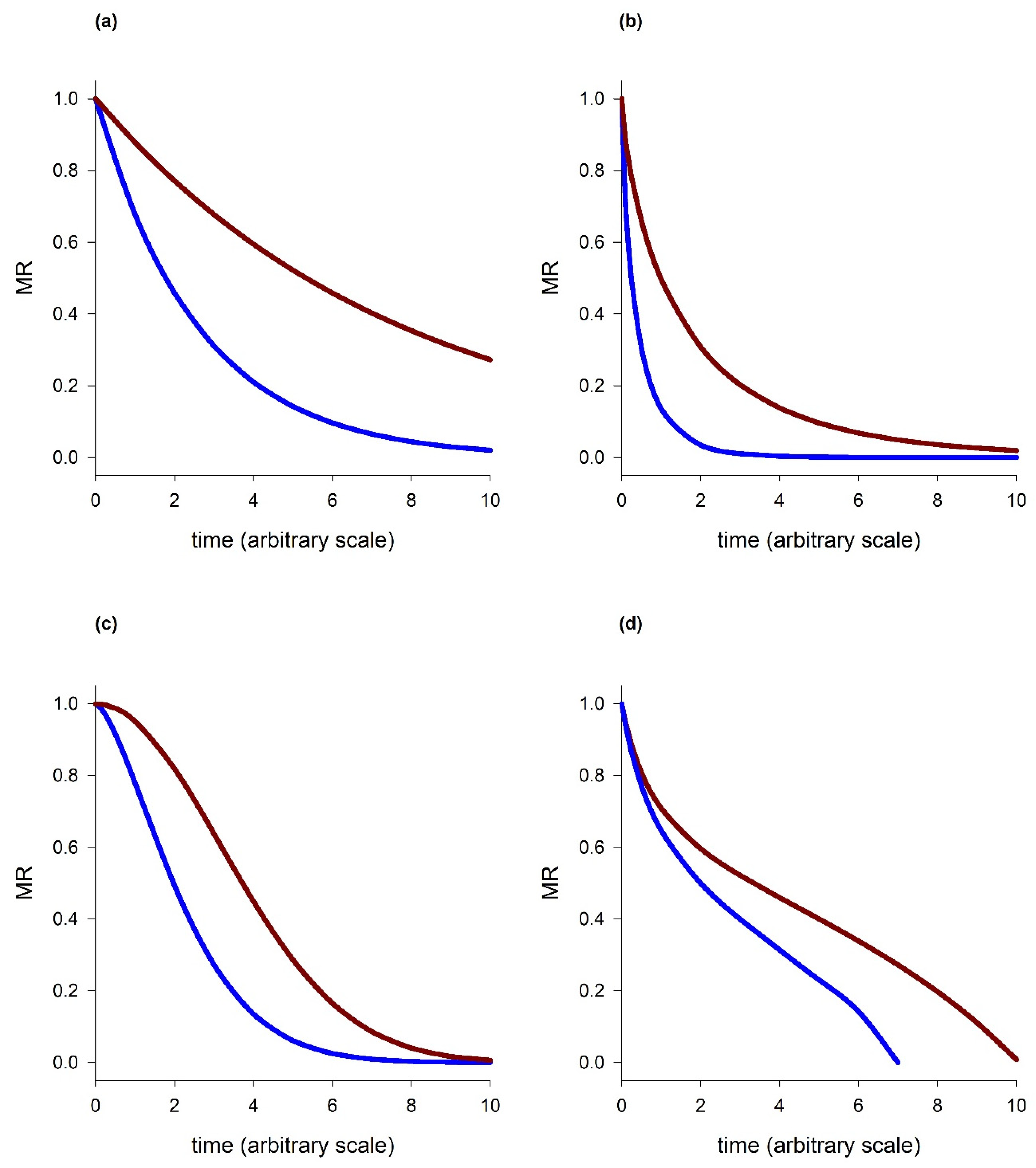
2. Types of Drying Curves

A careful inspection of the drying data available in literature suggested that the number of drying curves is limited and, in general, can be divided into four categories that are simulated in Figure 1: (i) concave (tailing) curves, which are simple exponential decaying curves (Figure 1a); (ii) strong tailing curves, which are similar to concave curves, though their initial period is much steeper (Figure 1b); (iii) sigmoid-type I or slightly convex followed by concave curves (Figure 1c); and (iv) sigmoid-type II or concave followed by slight convex curves (Figure 1d). Concave and strong tailing curves are too numerous to list. On the other hand, sigmoid curves (either type I or II) are rarely observed. Sigmoid-type I curves can be seen from Sadeghi et al. [5], although the convex (or shoulder) section is slightly observable (see also Figure 1c). Sigmoid-type II curves can be seen from Zhu and Shen [19].

Sadeghi et al. [5] listed 100 models, including feed-forward neural networks that could be used for thin-layer modeling. In fact, most of the drying curves can be described by models with only two adjustable parameters; therefore, we will try to answer “Are all of those models proposed for drying data necessary to describe the limited number of curves?” or “Can we eliminate some of those models and focus more on the secondary modeling, i.e., the effect of temperature on the primary model’s parameters?”. However, before that, we will discuss modifications of the existing models, the transformation of drying data and the use of complex models to eliminate some of those models.

3. Modification of the Models

Models proposed to use drying curves are sometimes modified. These modifications may result in better parameter properties, such as fewer correlations between the parameters, and they may also be useful to avoid convergence failure; however, these modifications lead to no improvement in the original model’s fit in the case of drying modeling. Let us consider the Page model [20]:

$$MR=\exp \left(-k·t^n\right)$$

(1)

where MR is the moisture ratio (dependent variable) and t is the time (independent variable). The model has two parameters (k and n) and can be used to describe many drying curves—these curves are shown in Figure 1a–c. This model can be modified as such:

$$MR=\exp \left[-{\left(K·t\right)}^n\right]$$

(2)

Equation (2), which is known as the modified Page [21] model, also has two parameters (K and n), and note that $k=K^n$. It can be said that both models, without any calculation, should have identical fits with the same parameter n, R² and RMSE values, since n determines the shape—see below (unfortunately, in some published studies, the results of the Page model [Equation (1)] and modified Page model [Equation (2)] differ, which is unacceptable). The only difference should be the values of k and K.

Published data were used to show the application of the models. These datasets were selected because (i) they are at different temperatures (min: 50 °C, max: 80 °C), (ii) air velocities (min: 0.5 m/s, max: 1.3 m/s) and (iii) thickness (min: 3 mm, max: whole fruit), (iv) they have a different number of data points (min: 8, max: 35) and (v) their time-scales are different (min: 75 min, max: 720 min). The fits of both models (Page and modified Page) are shown in Figure 2 for one dataset. The Page or modified Page model produced a reasonable fit visually, although the last two data points seemed to be the outliers. Furthermore, R² = 0.9960 and RMSE = 0.0192 also revealed a good fit to the data. The parameter values were obtained as k = 0.0227 ± 0.0023^a, K = 0.0331 ± 0.0005^a and n = 1.1102 ± 0.0288^a, where superscript a is the standard error. The results of all datasets for the Page and modified Page models are presented in

Table 1. Result of the fit of the Page [Equation (1)] and modified Page [Equation (2)] models to the published data.

Sample	T (°C)	Air Velocity (m/s)	Thickness (mm)	Page	Modified Page	R2	RMSE	Reference
Apple	50	1.3	5.0	k = 0.0023 ± 0.0003 n = 1.3182 ± 0.0295	K = 0.0098 ± 0.0001 n = 1.3182 ± 0.0295	0.9988	0.0142	[22]
Apricot	70	0.5	Whole fruit	k = 0.0018 ± 0.0002 n = 1.1445 ± 0.0226	K = 0.0039 ± 5.3 × 10−5 n = 1.1445 ± 0.0226	0.9963	0.0216	[23]
Peach	65	0.8	3.5	k = 0.0083 ± 0.0019 n = 1.1237 ± 0.0519	K = 0.0141 ± 0.0004 n = 1.1237 ± 0.0519	0.9973	0.0196	[24]
Peach	60	0.946	3.0	k = 0.0227 ± 0.0023 n = 1.1102 ± 0.0288	K = 0.0331 ± 0.0005 n = 1.1102 ± 0.0288	0.9960	0.0192	[19]
Pear	80	1.3	5.0	k = 0.0042 ± 0.0007 n = 1.3205 ± 0.0395	K = 0.0158 ± 0.0003 n = 1.3182 ± 0.0295	0.9984	0.0175	[22]

. As expected, both models had the same fit, meaning that they are not rival models. Therefore, fitting these models to the same data and comparing them is meaningless. However, unfortunately, this was the case for many published studies. Admittedly, the correlation between the parameters of the modified Page model [Equation (2)] was low, whereas parameter correlations were high for the Page model [Equation (1)], although this had no effect on parameter estimation. Moreover, the errors on K (for modified Page) were less than the errors on k (Page model)—see Table 1. It could be said that a modification of the Page model can improve the correlation between the parameters, but it certainly has no effect on the model’s fit.

Another modification of the Page model [Equation (1)] is the following [25]:

$$MR=\exp \left\{-{\left[k·\left(\frac{t}{L^2}\right)\right]}^n\right\}$$

(3)

Once again, without any calculation, this model should have the same fit with the Page and modified Page models (n also determines the shape here) and should also have the same R². The values of RMSE will be different because now we have three parameters (k, L and n) not two. However, using a complex model with the identical fit is not a valid option; therefore, this modification is not reasonable.

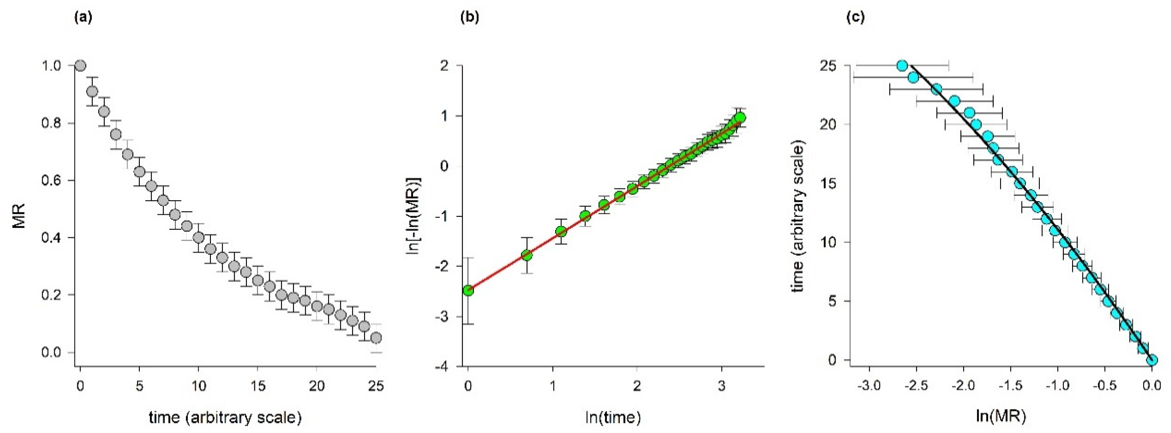
4. Models That Require Transformation

Some models that are used to describe drying data require transformation, where, data [whether dependent (MR) or independent (t) variable] are first transformed and then the regression is applied. However, the transformation of the dependent variable changes the error structure of the data [26]. Drying data of foods can be considered as homoscedastic (see the data of Lutovska et al. [27], and Turan and Fıratlıgil [28]) and transformation can make the data heteroscedastic. Hence, the models that require transformation should be used with caution.

Two frequently used models requiring transformation to describe drying data are the Diamante [29] and Thompson [30] models:

$$\ln \left(-\ln MR\right)=a+b·\ln t+c·{\left(\ln t\right)}^2$$

(4)

$$t=a·\ln MR+b·{\left(\ln MR\right)}^2$$

(5)

In the Diamante model [Equation (4)], the double logarithm of MR is used with a logarithmic transformation of t, and in the Thomson model [Equation (5)], the independent variable (t) and logarithmic transformation of the dependent variable (MR) are replaced. Linear regression can be applied since both models are linear in their parameters. Diamante et al. [29] also admitted that the aim of the transformation is to use polynomial regression (i.e., linear regression), which is available in almost all software and also some scientific calculators. In the case of drying data, however, there is no reason for transformation [22], and software/freeware for non-linear regression are accessible for everyone nowadays.

Synthetic but realistic drying data (MR versus t) were generated with equal uncertainty (error bar) for each datum point in order to investigate how transformation affects the error structure. Common practice in the modeling studies of drying data is to report the average values without the standard deviations; even the replicate measurements are available. Hence, it is not easy to find published drying data with uncertainties. Even if the error bars are available, it is also not easy to digitize and extract such data; therefore, synthetic homoscedastic data were used to show the effect of transformation. The results are presented in Figure 3.

It is clear that both models changed the error structure of the original data which were initially homoscedastic (Figure 3a). In the Diamante model [Equation (4)], at low time values, high errors were observed, and as time increased (so did lnt), errors were reduced to a certain period, and then increased again (Figure 3b). On the other hand, as time increased, errors increased for the Thomson model [Equation (5)] (Figure 3c). It can be said that the transformation carried out for both models ended up with heteroscedastic data, which is unwanted [26]. In conclusion, models that require transformation should not be used for drying data, or the heteroscedasticity of the data should be taken into account after the transformation; otherwise, regression will be flawed [31].

5. Use of Complex Models for Drying Data

In this section, we tried to fit some complex models to published drying data of some fruits, such as apple, pear and peach, and we also commented on those fits. By complex, we mean that the models have at least three or more adjustable parameters.

The first model used was the modified Henderson and Pabis equation [32], which is given below:

$$MR=a·\exp \left(-k·t\right)+b·\exp \left(-g·t\right)+c·\exp \left(-h·t\right)$$

(6)

Equation (6) with six parameters (a, k, b, g, c and h) was used for all datasets given in Table 1, and the parameter values with their standard errors and the goodness-of-fit indices (R² and RMSE) were obtained. R² values were between 0.9880–0.9946 and RMSE values were between 0.0285–0.0609. The model also fitted well to the data visually, which is shown in Figure 4 for one dataset. However, these can be misleading because some of the parameters in the model were statistically insignificant (p > 0.05) and there is no reason to use a complex model. In fact, parameters k and h were insignificant (p > 0.05) for all datasets, and in three out of the five data sets, parameter g was also insignificant together with k and h. This is also shown in

Table 2. Parameter estimates, standard errors and p values of the modified Henderson and Pabis equation [Equation (6)] to the data shown in Figure 4.

Parameter	Estimate	Standard Error	p Value
a	0.3369	0.0406	<0.0001
k	0.0343	0.0869	0.6994
b	0.3486	0.0580	<0.0001
g	0.0343	0.3713	0.9278
c	0.3364	0.0580	<0.0001
h	0.0343	0.3583	0.9251

for the same data set given in Figure 4.

The statistical significance of a single parameter in a model equation can be established by looking at the p value (the probability of being wrong in concluding that there is a relationship between the dependent and independent variables). Traditionally, p values higher than 0.05 indicate a statistically insignificant association between dependent and independent variables [33].

The second equation was a two-term model [34], which is similar to the modified Henderson and Pabis model but has fewer parameters:

$$MR=a·\exp \left(-k·t\right)+b·\exp \left(-g·t\right)$$

(7)

The question arises “does the two-term model [Equation (7)], with four parameters, have a satisfactory fit and significant parameters for the same datasets, or does it not?” Therefore, we tried this model, as we did the modified Henderson and Pabis model before. The R² values were again between 0.9880–0.9946 and the RMSE values were between 0.0266–0.0527. The model [Equation (7)] had an identical fit (with the same R² but slightly lower RMSE because it has a lower number of parameters. It is also unfortunate that, in most drying studies, RMSE is defined with only the number of data points; however, the number of parameters in the models should also exist in the formula [35]), and for four out of the five data sets parameters, k and g were insignificant (p > 0.05). In addition, in one data set, all parameters (a, k, b and g) were statistically significant (p ≤ 0.05).

Table 3. Parameter estimates, standard errors and p values of the two-term model [Equation (7)] to the data shown in Figure 4.

Parameter	Estimate	Standard Error	p Value
a	0.5134	0.0380	<0.0001
k	0.0343	0.1004	0.7372
b	0.5085	0.0542	<0.0001
g	0.0343	0.5067	0.9469

shows the results for the same data set given in Figure 4.

One can argue that both the Henderson–Pabis and the two-term models have similar structures and that it may not be surprising that both can have insignificant parameters. Hence, as a third equation, we proposed to use the Midilli model [36], which also has four parameters (a, k, n and b):

$$MR=a·\exp \left(-k·t^n\right)+b·t$$

(8)

For the same datasets, the R² values were between 0.9990–0.9996 and the RMSE values were between 0.0071–0.0146, indicating that the Midilli model [Equation (8)] produced a much better fit than the previous models. Parameter b was insignificant (p > 0.05) in only two out of the five cases, and all other parameters were significant (p ≤ 0.05). The fit is shown in Figure 5 together with the other models in this section, and

Table 4. Parameter estimates, standard errors and p values of the Midilli–Küçük model [Equation (8)] to the data shown in Figure 5.

Parameter	Estimate	Standard Error	p Value
a	0.9984	0.0098	<0.0001
k	0.0319	0.0036	<0.0001
n	0.9688	0.0361	<0.0001
b	−0.0012	0.0002	<0.0001

presents the parameter values and standard errors in which all parameters were significant (p ≤ 0.05).

The results presented here revealed that the complex models should be used with caution because parameters can be insignificant, and a simpler model with significant parameters can be used instead with the same degree of fit or with a slight loss of goodness-of-fit. It should also be noted that the significances of the parameters are highly dependent on the dataset and model structure. Nevertheless, it could be said that the simple models (models with or fewer than three adjustable parameters) should be preferred for the drying of foods.

Two problems may further arise if there are many parameters in a model equation: (i) Available programs for non-linear regression generally obtain the parameter values by minimizing the sum of square errors between experimental data and model fits (least-squares method) and may require the initial estimate of the parameters. Since the non-linear regression is an iterative procedure, the initial values for each parameter should be entered to start the iteration [37]. If the initial values are poorly selected, software cannot find a solution (known as convergence failure) within the iteration range. (ii) There is a possibility that the final values of the parameters found by the program do not belong to the best fit. This is due to obtaining a false or local minimum and is usually not a problem when only one or two parameters are being fit [38].

6. Models Proposed for Drying of Foods

Before proposing the models to be used for the drying of foods, we would like to summarize the results up until now, and we would also like to answer the question that we have asked in Section 2. There is no reason to use all the models available for drying data. The following models can be safely eliminated without hesitation:

(i)

Models that require transformed data;

(ii)

Complex models or models that have more than three parameters;

(iii)

Models that have the same fit with another model but have more parameters.

Moreover, it is known that when t = 0, MR = 1, and when t → ∞, MR → 0; hence, the models that do not satisfy the initial and final conditions can be eliminated too. Let us consider two models given below:

$$MR=\exp \left(-k·t\right)$$

(9)

$$MR=a·\exp \left(-k·t\right)$$

(10)

According to Equation (10), when t = 0, MR = a, and, as can be guessed, parameter a should be obtained by a regression that is as close to 1 (according to our results, the a values were always > 0.99). Equation (10) has some flexibility compared to Equation (9), where the initial condition is satisfied. Nevertheless, this model was eliminated because of the initial condition failure, and the same was also applied for the models that do not satisfy the final condition.

The thin-layer models eliminated and reasons for this elimination are listed in

Table 5. Eliminated thin-layer drying models and the reasons for this elimination.

Model No.	Model Name	Model Equation	Reason	Reference
1	Henderson–Pabis	$MR=a·\exp \left(-k·t\right)$	Initial condition	[40]
2	Modified Henderson–Pabis	$MR=a·\exp \left(-k·t\right)+b·\exp \left(-g·t\right)+c·\exp \left(-h·t\right)$	Initial condition Insignificant parameters	[32]
3	Modified Page II	$MR=\exp \left\{-{\left[k·\left(\frac{t}{L^2}\right)\right]}^n\right\}$	Simpler version with the same fit but fewer parameters is available	[25]
4	Logarithmic (Asymptotic)	$MR=a·\exp \left(-k·t\right)+c$	Initial condition Final condition	[41]
5	Midilli	$MR=a·\exp \left(-k·t^n\right)+b·t$	Initial condition Final condition Insignificant parameters	[36]
6	Modified Midilli I	$MR=\exp \left(-k·t^n\right)+b·t$	Final condition Insignificant parameters	[42]
7	Modified Midilli II	$MR=a·\exp \left(-k·t^n\right)+b$	Initial condition Final condition Insignificant parameters	[43]
8	Two-term	$MR=a·\exp \left(-k·t\right)+b·\exp \left(-g·t\right)$	Initial condition Insignificant parameters	[34]
9	Modified two-term I	$MR=a·\exp \left(-k·t\right)+\left(1-a\right)·\exp \left(-k·b·t\right)$	Insignificant parameters	[44]
10	Modified two-term II	$MR=a·\exp \left(-k·t\right)+\left(1-a\right)·\exp \left(-g·t\right)$	Insignificant parameters	[45]
11	Diamante	$\ln \left(-\ln MR\right)=a+b·\ln t+c·{\left(\ln t\right)}^2$	Transformation Heteroscedastic data	[29]
12	Thompson	$t=a·\ln MR+b·{\left(\ln MR\right)}^2$	Transformation Heteroscedastic data	[30]
13	Wang–Singh	$MR=1+b·t+a·t^2$	Final condition	[46]
14	Aghbashlo	$MR=\exp \left(-\frac{k_1·t}{1+k_2·t}\right)$	Final condition	[47]

. Those models can still be used; however, researchers who will use those models should be aware of the drawbacks. Initial (t = 0, MR = 1) and final (t → ∞, MR → 0) conditions may not be big issues but using the models with insignificant parameters is not a valid option and should be avoided. Another remark is that the models that were commented on as “insignificant parameters” in Table 5 may be specific to our datasets. Nevertheless, the probability of obtaining insignificant parameters is high and, therefore, these models should be checked by the researchers before presenting the results.

Suggested models for thin-layer drying are given in

Table 6. Suggested thin-layer drying models.

Model No.	Model Name	Model Equation	Comment	Reference
1	Lewis (Newton)	$MR=\exp \left(-k·t\right)$	Simplest model, but not flexible enough to describe many drying data	[39]
2	Page *	$MR=\exp \left(-k·t^n\right)$	Simple, and can be used to describe drying data of many foods. Strong correlation between the parameters.	[20]
3	Modified Page I *	$MR=\exp \left[-{\left(K·t\right)}^n\right]$	Same fit with the Page model; however, it has fewer errors on the rate parameter (K), and also correlation between the parameters are low.	[21]
4	Weibull *	$MR=\exp \left[-{\left(\frac{t}{\alpha }\right)}^{\beta }\right]$	Same fit with the Page model, low parameter correlation (same as Modified Page I).	[49]
5	Weibull I *	$MR={10}^{-{\left(\frac{t}{\delta }\right)}^n}$	Same fit with the Page model, mild parameter correlation. Interpretable time parameter (δ) that can be roughly estimated by visual inspection of the data.	[22]
6	Modified two-term III	$MR=a·\exp \left(-k·t\right)+\left(1-a\right)·\exp \left(-k·a·t\right)$	Mild to strong parameter correlation	[50]

* These models have the same fit; therefore, use of one of them is sufficient.

. The simplest model on the list was the Lewis or Newton model [39] because they only have one parameter but being simple does not always mean being the best. The Lewis model has a limited usage because it may be only used for the curves shown in Figure 1a. Some of the models given in Table 6 have exactly the same fit with each other; therefore, using one of them should be enough. Another important remark is that the meaning of the parameters should be well understood so that their effect on the shape of the drying curve can be established. See the following model for example:

$$MR={10}^{-{\left(\frac{t}{\delta }\right)}^n}$$

(11)

This model only has two parameters (δ and n), and it also satisfies the initial and final conditions. Hence, it can be used to describe the drying data of fruits and vegetables [22,48]. Moreover, it produces the same fit with the Page (or the Modified Page) and the Weibull model given in Table 6 as mentioned above, but the question that arises here is whether the parameters have a physical significance or not. The effect of different parameter values on the curve’s shape is demonstrated in Figure 6. Parameter n is the shape parameter because, if n < 1, the drying curve has a strong tailing, if n = 1, it is concave (or tailing) and if n > 1, then it has a sigmoid-type I shape (Figure 6a). Parameter δ is the time (its unit can be min or h) necessary to reduce the initial MR (1.0) to MR/10 (0.1). In Figure 6a, δ = 4; therefore, all curves intersect at t = 4 MR = 0.1 regardless of the value of the shape parameter, and, in Figure 6b, δ was set to 2, 4 and 8, respectively; hence, each curve passed t = 2 MR = 0.1, t = 4 MR = 0.1 and t = 8 MR = 0.1, respectively. It should be admitted that not all parameters in a model could have a specific or interpretable meaning as in this example. Nonetheless, researchers should try to understand the effects of parameters on the shape of the curve, and a simulation by using different parameter values can be very beneficial for this purpose.

7. Conclusions

This study reviewed some of the thin-layer drying models that are commonly used to describe the drying kinetics of different foods. The main conclusions are:

–

The arbitrary use of thin-layer drying models should be avoided;

–

Complex models, most of the time, result in insignificant parameters;

–

Models with two adjustable parameters work well for drying data;

–

Logarithmic transformation generates heteroscedastic data and should not be used.

Moreover,

• Drying data should not be presented with only the average values. Even using the average values with the error bars is not a good choice [37,51]. Instead, all genuine replicates should be entered, and the data should be modeled as such, since the replicates are generally independent [37];
• The simplest possible model that can describe the data should be considered as the best model (known as Ockham’s razor or rule of parsimony). Most drying data can be described with the two-parameter models. Therefore, it is best to try them first. More complex models should only be used if the simple model is not adequate to describe the data;
• Two different forms of the same models (having the same number of parameters) should not be used together because they are not rival models but the same models with different mathematical structures. The one that has less uncertainty on parameters and also a correlation between the parameters could be preferred;
• Parameters should also be listed together with their standard errors or confidence intervals, since uncertainties could also give information on the parameters’ significance;
• The meaning of the parameters and the effect of their values on the curve’s shape should be well known, even if the model used is an empirical one;
• The R² alone is not adequate to compare the models, and the RMSE and residuals should also be used to compare the models with the same number of parameters. A comparison of the models that have a different number of parameters (i.e., comparing a three-parameter model with a two-parameter model) may require different analyses, such as the F-test.

After selecting a suitable model or models, more efforts can be focused on finding secondary models. This would also lead to the prediction of drying curves under non-isothermal conditions, which is usually the case in microwave drying.

References

1. Babalis, S.J.; Papanicolaou, E.; Kyriakis, N.; Belessiotis, V.G. Evaluation of thin-layer drying models for describing drying kinetics of figs (Ficus carica). J. Food Eng. 2006, 75, 205–214. [Google Scholar] [CrossRef]
2. Kamal, M.M.; Ali, M.R.; Shishir, M.R.I.; Mondal, S.C. Thin-layer drying kinetics of yam slices, physicochemical, and functional attributes of yam flour. J. Food Process Eng. 2020, 43, e13448. [Google Scholar] [CrossRef]
3. Shishir, M.R.I.; Karim, N.; Bao, T.; Gowd, V.; Ding, T.; Sun, C.; Chen, W. Cold plasma pretreatment—A novel approach to improve the hot air drying characteristics, kinetic parameters, and nutritional attributes of shiitake mushroom. Dry. Technol. 2020, 38, 2134–2150. [Google Scholar] [CrossRef]
4. İlter, I.; Akyıl, S.; Devseren, E.; Okut, D.; Koç, M.; Kaymak Ertekin, F. Microwave and hot air drying of garlic puree: Drying kinetics and quality characteristics. Heat Mass Transf. 2018, 54, 2101–2112. [Google Scholar] [CrossRef]
5. Sadeghi, E.; Movagharnejad, K.; Asl, A.H. Mathematical modeling of infrared radiation thin-layer drying of pumpkin samples under natural and forced convection. J. Food Process. Preserv. 2019, 43, e14229. [Google Scholar] [CrossRef]
6. Keey, R.B. Drying Principles and Practice; Pergamon Press: Oxford, UK, 1972; pp. 1–18. [Google Scholar]
7. Klemes, J.; Smith, R.; Kim, J.K. Handbook of Water and Energy Management in Food Processing; Woodhead Publishing: Cambridge, UK; CRC Press: Boca Raton, FL, USA, 2008; pp. 449–629. [Google Scholar]
8. Onwude, D.I.; Hashim, N.; Janius, R.B.; Nawi, N.M.; Abdan, K. Modeling the thin-layer drying of fruits and vegetables: A review. Compr. Rev. Food Sci. Food Saf. 2016, 15, 599–618. [Google Scholar] [CrossRef] [PubMed]
9. Giri, S.K.; Prasad, S. Drying kinetics and rehydration characteristics of microwave vacuum and convective-hot air-dried mushrooms. J. Food Eng. 2007, 78, 512–521. [Google Scholar] [CrossRef]
10. Erbay, Z.; Icier, F. A review of thin layer drying of foods: Theory, modeling, and experimental results. Crit. Rev. Food Sci. Nutr. 2009, 50, 441–464. [Google Scholar] [CrossRef] [PubMed]
11. Sopade, P.A.; Xun, P.Y.; Halley, P.J.; Hardin, M. Equivalence of the Peleg, Pilosof and SinghKulshrestha models for water absorption in food. J. Food Eng. 2007, 78, 730–734. [Google Scholar] [CrossRef]
12. Bryś, A.; Kaleta, A.; Górnicki, K.; Głowacki, S.; Tulej, W.; Bryś, J.; Wichowski, P. Some Aspects of the Modelling of Thin-Layer Drying of Sawdust. Energies 2021, 14, 726. [Google Scholar] [CrossRef]
13. Kaleta, A.; Górnicki, K. Some remarks on evaluation of drying models of red beet particles. Energy Convers. Manag. 2010, 51, 2967–2978. [Google Scholar] [CrossRef]
14. Ashtiani, S.-H.M.; Salarikia, A.; Golzarian, M.R. Analyzing drying characteristics and modeling of thin layers of peppermint leaves under hot-air and infrared treatments. Inf. Process. Agric. 2017, 4, 128–139. [Google Scholar]
15. Górnicki, K.; Kaleta, A.; Choińska, A. Suitable model for thin-layer drying of root vegetables and onion. Int. Agrophys. 2020, 34, 79–86. [Google Scholar] [CrossRef]
16. Ertekin, C.; Firat, M.Z. A comprehensive review of thin-layer drying models used in agricultural products. Crit. Rev. Food Sci. Nutr. 2017, 57, 701–717. [Google Scholar] [CrossRef] [PubMed]
17. Van Boekel, M.A.J.S. Statistical aspects of kinetic modeling for food science problems. J. Food Sci. 1996, 61, 477–485, 489. [Google Scholar] [CrossRef]
18. Jayas, D.S.; Cenkowski, S.; Pabis, S.; Muir, W.E. Review of thin-layer drying and wetting equations. Dry. Technol. 1991, 9, 551–588. [Google Scholar] [CrossRef]
19. Zhu, A.; Shen, X. The model and mass transfer characteristics of convection drying of peach slices. Int. J. Heat Mass Transf. 2014, 72, 345–351. [Google Scholar] [CrossRef]
20. Page, G.E. Factors Influencing the Maximum Rate of Air Drying Shelled Corn in Thin-Layers. Master’s Thesis, Purdue University, West Lafayette, Indiana, 1949. [Google Scholar]
21. Overhults, D.G.; White, G.M.; Hamilton, H.E.; Ross, I.J. Drying soybeans with heated air. Trans. ASAE 1973, 16, 112–113. [Google Scholar] [CrossRef]
22. Karacabey, E.; Buzrul, S. Modeling and predicting the drying kinetics of apple and pear: Application of the Weibull model. Chem. Eng. Commun. 2017, 204, 573–579. [Google Scholar] [CrossRef]
23. Toğrul, İ.T.; Pehlivan, D. Modelling of drying kinetics of single apricot. J. Food Eng. 2003, 58, 23–32. [Google Scholar] [CrossRef]
24. Kingsly, R.P.; Goyal, R.K.; Manikantan, M.R.; Ilyas, S.M. Effects of pretreatments and drying air temperature on drying behaviour of peach slice. Int. J. Food Sci. Technol. 2007, 42, 65–69. [Google Scholar] [CrossRef]
25. Diamante, L.M.; Munro, P.A. Mathematical modelling of the thin layer solar drying of sweet potato slices. Sol. Energy 1993, 51, 271–276. [Google Scholar] [CrossRef]
26. Van Boekel, M.A.J.S. Kinetic Modeling of Reactions in Foods; CRC Press: Boca Raton, FL, USA, 2008. [Google Scholar]
27. Lutovska, M.; Mitrevski, V.; Pavkov, I.; Mijakovski, V.; Radojčin, M. Mathematical modelling of thin layer drying of pear. Chem. Ind. Chem. Eng. Q. 2016, 22, 191–199. [Google Scholar] [CrossRef]
28. Turan, O.Y.; Fıratlıgil, F.E. Modelling and characteristics of thin layer convective air-drying of thyme (Thymus vulgaris) leaves. Czech J. Food Sci. 2019, 37, 128–134. [Google Scholar] [CrossRef]
29. Diamante, L.M.; Ihns, R.; Savage, G.P.; Vanhanen, L. A new mathematical model for thin layer drying of fruits. Int. J. Food Sci. Technol. 2010, 45, 1956–1962. [Google Scholar] [CrossRef]
30. Thompson, T.L.; Peart, R.M.; Foster, G.H. Mathematical simulation of corn drying—A new model. Trans. ASAE 1968, 11, 582–586. [Google Scholar] [CrossRef]
31. Schaffner, D.W. Predictive food microbiology Gedanken experiment: Why do microbial growth data require a transformation? Food Microbiol. 1998, 15, 185–189. [Google Scholar] [CrossRef]
32. Karathanos, V.T. Determination ofwater content of dried fruits by drying kinetics. J. Food Eng. 1999, 39, 337–344. [Google Scholar] [CrossRef]
33. Buzrul, S. Letter to the Editor: Models with Insignificant Parameters. Appl. Environ. Microbiol. 2008, 74, 6481–6482. [Google Scholar] [CrossRef] [Green Version]
34. Henderson, S.M.; Pabis, S. Grain drying theory I: Temperature effect on drying coefficient. J. Agric. Eng. Res. 1961, 6, 169–174. [Google Scholar]
35. Buzrul, S.; Alpas, H. Modeling the synergistic effect of high pressure and heat on the inactivation kinetics of Listeria innocua: A preliminary study. FEMS Microbiol. Lett. 2004, 238, 29–36. [Google Scholar] [PubMed]
36. Midilli, A.; Kucuk, H.; Yapar, Z. A new model for single-layer drying. Dry. Technol. 2002, 20, 1503–1513. [Google Scholar] [CrossRef]
37. Motulsky, H.J.; Christopoulos, A. Fitting models to biological data using linear and nonlinear regression. In A Practical Guide to Curve Fitting; GraphPad Software Inc.: San Diego, CA, USA, 2003. [Google Scholar]
38. Motulsky, H.J.; Ransnas, L.A. Fitting curves to data using nonlinear regression: A practical and nonmathematical review. FASEB J. 1987, 1, 365–374. [Google Scholar] [CrossRef] [PubMed]
39. Lewis, W.K. The rate of drying of solid materials. IEC-Symp. Dry. 1921, 3, 427–432. [Google Scholar] [CrossRef]
40. Henderson, S.M. Progress in developing the thin layer drying equation. Trans. ASAE 1974, 17, 1167–1172. [Google Scholar] [CrossRef]
41. Yagcioglu, A.; Degirmencioglu, A.; Cagatay, F. Drying characteristics of laurel leaves under different drying conditions. In Proceedings of the 7th International Congress on Agricultural Mechanization and Energy, Adana, Turkey, 26–27 May 1999; pp. 426–431. [Google Scholar]
42. Ghazanfari, A.; Emami, S.; Tabil, L.G.; Panigrahi, S. Thin-layer drying of flax fiber: Modeling drying process using semi-theoretical and empirical models. Dry. Technol. 2006, 24, 1637–1642. [Google Scholar] [CrossRef]
43. Demir, V.; Gunhan, T.; Yagcioglu, A.K. Mathematical modelling of convection drying of green table olives. Biosys. Eng. 2007, 98, 47–53. [Google Scholar] [CrossRef]
44. Sharaf-Eldeen, Y.I.; Blaisdell, J.L.; Hamdy, M.Y. A model for ear corn drying. Trans. ASAE 1980, 23, 1261–1271. [Google Scholar] [CrossRef]
45. Verma, L.R.; Bucklin, R.A.; Ednan, J.B.; Wratten, F.T. Effects of drying air parameters on rice drying models. Trans. ASAE 1985, 28, 296–301. [Google Scholar] [CrossRef]
46. Wang, C.Y.; Singh, R.P. A Single Layer Drying Equation for Rough Rice; ASAE Paper No. 3001; ASAE: St. Joseph, MI, USA, 1978. [Google Scholar]
47. Aghbashlo, M.; Kianmehr, M.H.; Khani, S.; Ghasemi, M. Mathematical modeling of thin-layer drying of carrot. Intl. Agrophys. 2009, 23, 313–317. [Google Scholar]
48. Baltacıoğlu, C.; Okur, İ.; Buzrul, S. Model based comparison of drying of asparagus (Asparagus officinalis L.) with traditional method and microwave. J. Food 2020, 45, 572–580. [Google Scholar]
49. Corzo, O.; Bracho, N.; Pereira, A.; Vasquez, A. Weibull distribution for modeling air drying of coroba slices. LWT—Food Sci. Technol. 2008, 41, 2023–2028. [Google Scholar] [CrossRef]
50. Hutchinson, D.; Otten, L. Thin-layer air drying of soybeans and white beans. J. Food Technol. 1983, 18, 507–522. [Google Scholar] [CrossRef]
51. Van Boekel, M.A.J.S. To pool or not to pool: That is the question in microbial kinetics. Int. J. Food Microbiol. 2021, 354, 109283. [Google Scholar] [CrossRef] [PubMed]
Figure 1. Simulated drying curves: concave or tailing (a), strong tailing (b), sigmoid-type I (convex followed by concave) (c) and sigmoid-type II (concave followed by convex) (d).
Processes 10 00118 g001
Figure 2. Drying data of peach slices at 60 °C (gray circles). Solid line indicates the fit of Page [Equation (1)] or modified Page [Equation (2)] model, where R2 = 0.9960 and RMSE = 0.0192. Original data are from Zhu and Shen [19].
Processes 10 00118 g002
Figure 3. Synthetic drying data with equal error bars (a), fit of Diamante model—red line [Equation (4)] to the transformed data, where R2 = 0.9987 and RMSE = 0.0331 (b) and fit of Thompson model—black line [Equation (5)] to the transformed data, where R2 = 0.9966 and RMSE = 0.4546 (c).
Processes 10 00118 g003
Figure 4. Drying data of peach slices at 60 °C (gray circles). Solid line indicates the fit of modified Henderson–Pabis model [Equation (6)], where R2 = 0.9931 and RMSE = 0.0285. Original data are from Zhu and Shen [19].
Processes 10 00118 g004
Figure 5. Drying data of peach slices at 60 °C (gray circles). Solid blue line indicates the fit of modified Henderson–Pabis model [Equation (6)] (R2 = 0.9931 and RMSE = 0.0285) and two-term model [Equation (7)] (R2 = 0.9931 and RMSE = 0.0266). Dashed red line indicates the fit of Midilli model [Equation (8)] (R2 = 0.9989 and RMSE = 0.0104). Original data are from Zhu and Shen [19].
Processes 10 00118 g005
Figure 6. Effect of shape parameter (n) on the drying curves’ shape (a) and effect of time parameter (δ) on the drying curves’ shape (b) given by Equation (11). The unit of time is whether min or h.
Processes 10 00118 g006