Article

Simulations of Heat Supply Performance of a Deep Borehole Heat Exchanger under Different Scheduled Operation Conditions

1
Tianjin Geothermal Research and Training Center, College of Mechanical Engineering, Tianjin University, Tianjin 300350, China
2
Key Laboratory of Efficient Utilization of Low and Medium Grade Energy, MOE, College of Mechanical Engineering, Tianjin University, Tianjin 300350, China
3
Institute of Hydrogeology and Environmental Geology, Chinese Academy of Geological Sciences, Shijiazhuang 050061, China
*
Author to whom correspondence should be addressed.
Processes 2022, 10(1), 121; https://doi.org/10.3390/pr10010121
Submission received: 5 December 2021 / Revised: 2 January 2022 / Accepted: 5 January 2022 / Published: 7 January 2022

Abstract

:
With the changing world energy structure, the development of renewable energy sources is gradually accelerating. Among them, close attention has been given to geothermal energy because of its abundant resources and supply stability. In this article, a deep borehole heat exchanger (DBHE) is coupled with a heat pump system to calculate the heat supply and daily electricity consumption of the system. To make better use of the peaks and valleys in electricity prices, the following three daily operating modes were studied: 24-h operation (Mode 1), 8-h operation plus 16-h non-operation (Mode 2), and two cycles of 4-h operation and 8-h non-operation (Mode 3). Simulation results show that scheduled non-continuous operation can effectively improve the outlet temperature of the heat extraction fluid circulating in the DBHE. The heat extraction rates of Mode 1 is 190.9 kW for mass flowrate of 9 kg/s; in Mode 2 and Mode 3 cases, the rates change to 304.7 kW and 293.0 kW, respectively. The daily operational electricity cost of Mode 1 is the greatest because of 24-h operation; due to scheduled non-continuous operation, the daily operational electricity cost of Mode 3 is only about 66% of that of Mode 2. After an 8-month period without heating, the formation-temperature can be restored within 4 °C of its original state; 90% recovery of the formation-temperature can be achieved by the end of the second month of the non-operation season.

1. Introduction

To achieve the goal of an emission peak and carbon neutrality in China, it is necessary to change China’s energy structure and vigorously develop renewable energy sources. Geothermal energy will become the focus of renewable energy development in the future because of its advantages of large reserves, stability and cleanliness. Although geothermal energy reserves are large, modern technology can transform only a small part of these reserves into electric energy and heat energy for human use [1].
In geothermal energy, the reserves of hot dry rocks (HDR) are the largest, but the engineering applications of HDR are very few. Aghahosseini et al. [2] expounded on applying the existing theory and technology of enhanced geothermal energy (EGS) systems to dry hot rock and expressed their own views on the economy and development potential of the system. However, the maintenance of cracks, corrosion, and scaling of geothermal water in EGSs are urgent problems to be solved before applications to dry hot rock [3,4,5]. To solve these problems, Rybach et al. [6] first proposed the concept of deep borehole heat exchangers (DBHEs) in 1995. The DBHE system is composed of a coaxial heat exchanger, and water flows in pipes, avoiding direct contact with rock, which solves the corrosion problem of EGS, but the heat transfer is much smaller than EGS. To improve the heat transfer capability of DHBEs, a series of simulations and experiments have been carried out.
Dijkshoorn et al. [7] evaluated the cooling capacity of a 2500 m deep DBHE system located in the center of Aachen, Germany. The results show that the well can provide the required temperature for a short time, but if the system is operated for 20 years, it cannot drive the adsorption device to cool buildings to low temperatures. However, the system can still provide enough heat to buildings in winter. In the town of Penzlau, Sapinska-sliwa et al. [8] also conducted experimental studies on DBHE systems. In China, Xi’an Jiaotong University has established a demonstration project to study the thermal performance of DBHEs [9,10]. Due to high drilling costs, most researchers have carried out simulations of DBHEs.
To improve the heat transfer performance of DBHEs, Li et al. [11] replaced the inner smooth tube with a spiral tube and a corrugated tube. They concluded that the change of geothermal water flowrate and rock temperature has more influence than the shape of the inner pipe on the heat extraction capacity of the DBHE system. Ali et al. [12] replaced the inner tube of the coaxial heat exchanger with an eccentric tube and made the eccentric tube rotate. Research showed that the heat transfer efficiency reached 223% when the rotational speed was 500 rpm and the eccentricity was 40 mm; but at the same time, the pressure loss of the system also increased by 53%. For the influence of the ratio of the inner and outer diameters of DBHEs on the heat transfer performance, Mokhtari et al. [13] and Iry et al. [14] carried out a detailed study and reached similar conclusions. The research results of Mokhtari et al. [13] show that the system pressure drop is the largest when the diameter ratio is 0.675, and the system thermal efficiency is the highest when the diameter ratio is 0.353. Oh et al. [15] carried out an experimental study on coaxial heat exchangers with different tubes, diameters and grouting materials at a depth of 50 m. The results showed that the thermal conductivity of pipes and grouting materials directly affect the performance of coaxial heat exchangers. He et al. [16] improved the filler part of DBHE system by mixing graphene with mud and cement respectively. On this basis, simulations of DBHEs were gradually proposed. Fang et al. [17] developed a thermal analysis software package of a coaxial heat exchanger based on the finite difference method, which greatly improved the calculation efficiency by directly solving the algebraic equations. Naldi et al. [18] proposed an iterative method with uniform temperature and constant heat flux as boundary conditions to calculate the characteristics of a group of 3 × 2 coaxial heat exchangers. Song et al. [19] established an unsteady heat transfer model of a coaxial heat exchanger and analyzed the factors affecting the heat transfer effect. Luo et al. [20] established a segmented finite cylinder-source model (SFCS) for simulating the DBHE system and compared it with finite difference model. Beier [21] established a transient heat transfer model and verified it by measured vertical temperature profiles in a borehole and temperatures of previous simulations. Li et al. [22] established a model by MATLAB and verified it by an experiment located at the Chang’an District of Xi’an. The radius of influence of rock temperature change during one heat season is about 7 m and the linear meter heat extraction rates is less than 150 W. For the working fluid in DBHEs, Daneshipour [23] added two kinds of nanoparticles to water and carried out the corresponding research. The results showed that a CuO-water nanofluid had better heat transfer performance than an Al2O3-water nanofluid, but the pressure loss and axial power were higher for the CuO-water nanofluid than the Al2O3-water nanofluid.
Bu et al. [24] conducted a 138-day experiment of a DHBE in a geothermal well with a depth of 2605 m. The average heating capacity of the well was 448 kW. Bär et al. [25] used deep rock as an energy storage device to study the effect of storing heat with the temperature of rock exceeds 110 °C with a depth of 500–1500 m in the summer. The results show that this method can realize the operation of heating temperatures above 45 °C during the winter. Welsch et al. [26] conducted a similar study.
Although there has been much research on DBHE systems, study on the heat supply performance of a DBHE under different scheduled operation conditions is weak, and hence the reason why this research is carried out. Additionally, there are almost no integrated calculations of underground heat extraction, aboveground application, and the costs of operations. In view of the lack of research on these topics, this paper proposes three operational strategies for different building types and analyzes the heat transfer performance of DBHEs combined with heat pump systems. Additionally, the daily costs of different operating strategies are calculated according to the peaks and valleys in electricity prices in China. The results of this study can provide technical support for engineering applications of DBHEs.

2. Models and Methodology

In order to consider the decrease of the daily operation electricity cost of the system. A set of integrated system including underground Deep Borehole Heat Exchanger (DBHE) system and aboveground heat pump system has been built for winter heating of commercial buildings, with consideration of peak–valley electricity price. The DBHE model and heat pump model with governing equations are shown in Appendix A and Appendix B, respectively.
In this study, Fluent is used for DBHE simulation and the Engineering Equation Solver (EES) is used for heat pump system simulation.

2.1. DBHE Model and Validation

To research the heat extraction performance of DBHE systems, a 3-D model is established and verified by the demonstration project (Wang et al., 2019) located in Xi’an [9,10]. Figure 1 shows a simple diagram of the DHBE system.
As shown in Figure 1, water flows in the DBHE from the annular pipe. After extracting heat from rock, water is pumped out from the inner pipe in the heating season (four months during winter).
In this study, the equations of DBHE system are shown in Appendix A. In the DBHE model, the domain is set to be 100 m long, 100 m wide, and 2100 m deep. The depth of the well is 2000 m; there is a 100-m rock layer under the well. In terms of the meshes, denser grid is used around the well; the minimum grid size is 0.02 m and the width of each next grid increases by 1.5 times. In the depth direction, the grid size is set as 10 m considering the vertical geothermal temperature gradient is only 30 °C/km.
The boundary conditions are as follows:
  • Surface temperature is set to be 15.6 °C;
  • The inlet temperature of geothermal water is set to be 17.3 °C and the flow rate is set to be 28 m3/h;
  • The boundaries of the domain, expect the surface, are heat insulated boundaries.
The initial conditions are as follows:
  • The initial formation temperature profile is detaining by the surface temperature and geothermal temperature gradient (30 °C/km);
  • The initial water temperature in the well is set to be the same as the formation temperature distribution.
  • The initial pressure of water in the well is set to be its hydraulic pressure.
The following assumptions are also made in this model:
  • The parameters of the rock physical properties are symmetrical, thus a ¼-model is established to reduce the computation time.
  • The surface temperature is set to a constant value.
  • The contact thermal resistance between the rock and shaft wall is ignored.
According to these assumptions, a mesh of the 3-D model is established.
In the demonstration project [9], the formation is divided into four layers according to the field exploration data and the geological parameters of Shaanxi Province, and the physical parameters of each layer are shown in Table 1. The geothermal temperature gradient is 30 °C/km, the depth of the well is 2000 m and the depth of the inner pipe is 1998 m. A gap of 2 m is used for water (heat extraction fluid) to flow through. Material of Annular and inner pipe is shown in Table 2. During the test, the temperature of ground is 15.6 °C and the average inlet temperature of the water is 17.3 °C. The average flow is 28 m3/h.
The simulation results are shown in Figure 2a and the results of the experiment are shown in Figure 2b.
According to the results of the simulation of the system in Figure 2a, after one month of operation, the outlet temperature of water is 22.6 °C. Figure 2b shows the temperature during the last four days of a month of continuous operation of the demonstration project, and the average temperature is in the range of 25.4–26.8 °C [9]. The error is in the range of 2.8–4.2 °C. The most important factors are as follows. First, in the simulation, the temperature gradient is set as 30 °C/km, and it is slightly different in the demonstration project. Second, the thermal conductivity and other physical parameters of rock are set as constant in the simulation, but they vary with the depth and the radial direction of the well and cannot be completely consistent with the simulation. The simulation results are considered to be correct. The following study was carried out on this basis.
After validating the model, we also carried out a series of studies on different mass flows and operation modes. In these studies, the inlet temperature and the surface temperature of rock are 20 °C, the inner tube wall is insulation, the temperature gradient is 30 °C/km, the rock material is calcium carbonate, and the working fluid is water. The performance of different mass flow rates was compared.

2.2. Heat Pump Model

In China, the temperature of heating in winter should be higher than 40 °C, but the outlet temperature of geothermal water is lower, and thus heat pump systems are necessary. A heat pump system was modeled by an engineering equation solver (EES) software. The model governing equations are shown in Appendix B. In this system, the inlet and outlet temperatures of heating are 45 °C and 35 °C, respectively. The heat source temperature is the outlet temperature of geothermal water in Figure 1, and the heat source temperature changes to 20 °C after heat release at the evaporator. The working fluid is R123. The specific parameters of the heat pump system are shown in Table 3.

3. Operation Mode Description

In this paper, the heating season is four months, and the remaining eight months of the year are used for the temperature recovery of rock. According to different building types, we discuss three operation modes:
Mode 1: Running 24 h a day for buildings with all day heating demand.
Mode 2: Running 8 h and non-operation 16 h for residential buildings where there is a demand for heating at night.
Mode 3: Running for 4 h and non-operation for 8 h during the day, then running for 4 h and non-operation for 8 h at night, for commercial buildings, such as office buildings, where there is heating load during the day.
In this article, Mode 3 is designed for commercial buildings that need heating during the day (9:00–17:00). However, in China, there is a peak and valley electricity price policy, and the specific prices are shown in Table 4. Thus, for heating from 9:00 to 11:00, the price is 0.21 USD/kW·h, and for heating from 11:00 to 5:00, the price is 0.18 USD/kW·h. To take advantage of the electricity price of 0.07 USD/kW·h from 23:00 to 7:00, heat storage is combined with the DBHE. The specific operating strategy from 1:00 to 5:00 is to store energy as heat. During this period, the price of electricity is only 0.07 USD/kw·h. When buildings need heat from 9:00 to 13:00, energy is released from heat storage. Then, from 13:00–17:00, a heat pump system was used to heat the building directly. During this period, the price of electricity is 0.18 USD/kW·h. This operation mode effectively avoids running the heat pump system during the period of high electricity price.

4. Simulation Results

4.1. Comparison of Outlet Temperature

In this study, the formation is chosen to be CaCO3. The temperature of ground is set to be 20 °C and the inlet temperature is set to be 20 °C as well.
After four months of operation, the outlet temperature under different mass flow rates is shown in Figure 3. Figure 3a–c shows the results for Modes 1, 2, and 3, respectively. With the increase of mass flow, the time when the outlet temperature tends to be flat is gradually shortened. The reduction in outlet temperature gradually decreases with increasing mass flow. In Figure 3b,c, the outlet temperature fluctuates because when the DBHE stops operating, the temperature of the rock around the well rises, which causes the outlet temperature to rise during the next operating period. The temperature fluctuation range is approximately 7 °C for Mode 2 and 3 °C for Mode 3; they are determined by the length of time that the system is not running.
Table 5 shows the outlet temperatures for the three modes. It is obvious that scheduled non-continuous operation (Modes 2 and 3) can improve the outlet temperature efficiency. However, the outlet temperatures of Mode 2 and Mode 3 are very close when the mass flow is larger than 1 kg/s. The temperature difference between Modes 1, 2, and 3 decreases from approximately 14 °C to 3 °C as the mass flow changes from 1 kg/s to 9 kg/s. Comparing the numerical results for outlet temperature with time during, the simulation shows that the temperature difference of Mode 2 is greater than Mode 3. It is because Mode 2 has a longer shutdown time than Mode 3, which leads to a higher temperature of rock around the well, but the longer running time of Mode 2 eliminates this advantage. Thus, scheduled non-continuous operation can increase the outlet temperature, but redistributing the operating time has only a small effect on the outlet temperature.

4.2. Heat Extraction Capacity

In this research, the heat extraction capacity of a DBHE system is compared for three modes in two aspects: 1. heat extraction rates from wells, 2. heat extraction rates from the condenser of the heat pump system.

4.2.1. Heat Extraction Rates from Wells

Figure 4 clearly shows the values and comparison of the heat extraction rate from wells operating under different modes. Modes 2 and 3 greatly improve the heat extraction rates for different mass flows. Compared to Mode 1, the percentage increase of the heat extraction rates are 46.1%, 65.0%, 63.1%, 61.1%, and 59.6% for Mode 2 and 42.9%, 65.5%, 61.3%, 61.0%, and 53.5% for Mode 3 at the mass flow rates of 1, 3, 5, 7, and 9 kg/s, respectively. In Figure 5, the percentage increase of heat extraction rates from the condenser of the heat pump system basically unchanged.

4.2.2. Heat Extraction Rates from the Condenser of the Heat Pump System

During the heating season, the temperature of the building inlet is approximately 45 °C, thus most cases cannot directly heat buildings in three modes. To better compare the performance of the coupled heat pump system, all mass flows of the three modes are calculated by the EES. All calculation results are exhibited in Figure 5. Comparing Figure 4 and Figure 5 shows that the heat pump system can effectively improve the heat extraction rates. For Mode 1, the heat extraction rate increases from 22.2 to 33.5 kW with increasing mass flow. However, for Mode 2 and Mode 3, the growth range changes to 32.4–53.4 kW and 31.7–51.4 kW, respectively. However, with increasing heat extraction rates, the energy consumption of the working fluid pump also increases. More detailed data are shown in Table 6. According to these data, the energy consumption is greater for Modes 2 and 3 than Mode 1.

4.2.3. Comparison of Electricity Charge and Heat Extraction Rates of Mode 3

The electricity charge for the heat pump system running in the three modes for one day is shown in Table 7. In this table, because the system operates all day in Mode 1, the total price of operating the heat pump for one day is much greater than that for Modes 2 and 3. Although both Modes 2 and 3 operate for 8 h one day, Mode 2 runs from 9:00 to 17:00 and Mode 3 runs from 13:00–17:00 and 1:00–5:00. As shown in Table 4, different times have different electricity prices. Hence, the electricity price during the operation time of Mode 3 is lower than that of Mode 2. Through comparison, it is found that the electricity price of Mode 3 is 65.2%, 66.9%, 65.9%, 66.6% and 64.1% of that of Mode 2 for the mass flow increases from 1 kg/s to 9 kg/s. The percent is basically determined by the peak–valley electricity prices. Therefore, Mode 3 is the most suitable mode for commercial buildings.

4.3. Rock Temperature Change

To research the sustainable operation of the system, rock temperatures at different depths after the heating season and recovery during the other eight months were also studied.

4.3.1. Rock Temperature at Different Depths

Figure 6 shows the rock temperature at different depths after four months of operation in Mode 1. Results at four depths and five mass flows are displayed. The rock temperature decreases at every depth with increasing mass flow from 1 to 9 kg/s. The temperature difference between 1 and 3 kg/s is much larger than that of the other two adjacent mass flows. The reason is that when the mass flow is less than 3 kg/s, low velocity corresponds to low convective heat transfer coefficient, the heat conduction inside the rock can make up for the heat absorbed by the fluid. When the mass flow is greater than 3 kg/s, the heat conduction inside the rock is much smaller than the heat absorbed by the fluid, the rock thermal conductivity becomes the key limiting factor for geothermal heat extraction. At the same time, 8 m from the well, the rock temperature shows almost no change after four months of operation. A rock temperature comparison for the three modes is shown in Figure 7. Because the comparison of the same mass flow shows the same trend for the three modes, Figure 7 only shows the rock temperature for a mass flow rate of 9 kg/s. The tock temperature of Mode 3 is between those of Modes 1 and 2. The temperature near the well of Modes 2 and 3 is much higher than that of Mode 1. The cause of this phenomenon is that during the last period of four months of operation, Mode 1 runs full time, Mode 2 stops running for 16 h and Mode 3 stops running for 8 h. This leads to temperature recovery over different periods of time for Mode 2 and Mode 3.

4.3.2. Temperature Recovery of Rock

After four months of operation, the rock has a period of eight months of temperature recovery. Therefore, the temperature increase of rock month by month is researched. The results for Mode 1 are shown in Figure 8 and Figure 9. Figure 8 and Figure 9 show the temperature at depths of 1998 m and 1000 m, respectively, calculated as mass flows at 9 kg/s. These two figures show that the recovery of rock temperature is very obvious at the end of the first month of system non-operation. The temperature recovery effect gradually decreases with the passage of time. The difference between the rock temperature after eight months of system non-operation and the initial temperature of the rock is less than 4 °C. Similar conclusions are obtained in Modes 2 and 3, thus those figures are not shown.
The temperature change is shown in more detail for the rock temperature recovery at 1998 m deep for the three modes in Table 8. All data in Table 8 are based on a mass flow of 9 kg/s. At the end of eight months of system shutdown, the temperature difference of rock at 1998 m for the three modes is less than 1 °C. Subsequent calculations showed that the temperature recovery during the first month and the first two months accounted for 83% and 90% of the total temperature recovery during eight months for Mode 1, 79% and 88% for Mode 2, and 81% and 89%, for Mode 3, respectively. Thus, the rock temperature recovery was mainly concentrated in the first two months.

5. Conclusions

In this article, the heat extraction performance and formation temperature recovery characteristics of a 2000-m borehole heat exchanger with different heat-extraction mass flowrates were investigated in terms of three operational modes. Based on the analysis of the simulation results, the following results were obtained:
  • Comparing the outlet temperature of the heat extraction fluid (water) from the well for the three operating modes showed that the outlet temperatures, from high to low, were in the following order: Mode 2, Mode 3, and Mode 1. Heat extraction rates also maintained the same trend.
  • The heat pump system can effectively increase the final heat supply to the consumer, especially for Mode 2 and Mode 3. The increase percentage is about 60%. With increasing heat extraction rates, the heat pump power consumption also increases and is directly proportional to the heat supply.
  • The daily heat pump operational electricity cost in Mode 1 is the greatest because of the 24-h operation. Among the scheduled non-continuous operation modes, Mode 3 consumed about 66% of the daily electricity cost of Mode 2. Mode 3 is more suitable for commercial buildings.
  • The formation temperature recovery becomes slower over time during the non-operation season, and the difference between the final and the initial formation temperatures is only 4 °C or less; in other words, 90% recovery of formation-temperature can be achieved by the end of the second month of the non-operation season.

Author Contributions

J.Z., X.L. and W.Z. participated in the study concept, model and review of the manuscript; J.Z., J.L. and W.Y. participated in the model calculate; D.L., Q.M. and F.M. participated in the revive of the manuscript. All authors have read and agreed to the published version of the manuscript.

Funding

This research was funded by “Ministry of Science and Technology: 2019YFB1504105”.

Institutional Review Board Statement

Not applicable.

Informed Consent Statement

Not applicable.

Data Availability Statement

Not applicable.

Acknowledgments

The authors gratefully acknowledge the financial support provided by the National Key Research and Development Program of the 13th Five-Year Plan of China (No. 2019YFB1504105).

Conflicts of Interest

The authors declare no conflict of interest.

Appendix A. DBHE Model

The governing equations of DBHE in this study are shown as follow.
Continuity equation:
t ( ρ ) = z ( ρ v ) + m
where ρ is the density of water, kg/m3; v is the velocity of water, which is the rate of volume flow across the cross-sectional area of the annular or the inner pipe in this 1D equation, m/s; m is the mass sink/source term, kg/m3·s.
Momentum equation:
P z = ρ g cos ( θ ) ± f ρ v 2 2 d ± ( t ( ρ v ) + z ( ρ v 2 ) )
where P is the fluid pressure, Pa; g is the gravitational acceleration, m/s2; θ is the inclination of the well; f is the fraction factor; d is the wellbore hydraulic diameter, m.
Energy equation:
t ( ρ ( h P ρ + v 2 2 ) ) = z ( ρ v ( h + v 2 2 ) ) ρ v g cos ( θ ) q A + Q
where h is the enthalpy of water, kJ/kg; q is the lateral heat flow, W; Q is the heat sink/source term, W/m3. In the formula, z is the coordinate in vertical direction.
For inner pipe fluid, the heat flow is calculated by:
q = q 1 = A 1 U ( T 1 T 2 )
where q 1 is heat exchange rate between inner pipe flow and the annular flow, W; U is overall heat transfer coefficient between the inner pipe flow and annular flow, W/(m2·K); A 1 is the heat exchange area of the inner pipe inside surface, m2; T 1 is water temperature of inner pipe flow, K; T 2 is water temperature of annular flow, K.
U A 1 = π 1 2 a 1 r 1 + 1 2 λ 1 ln r 2 r 1 + 1 2 a 2 r 2
where a 1 is convective heat transfer coefficient corresponding to the inner pipe flow, W/(m2·K); r 1 is inner radius of inner pipe, m; λ 1 is thermal conductivity of the inner pipe material, W/(m·K); a 2 is convective heat transfer coefficient corresponding to the annular flow associated with the outer wall of the inner pipe, W/(m2·K); r 2 is outer radius of inner pipe, m.
For annular pipe fluid, the heat flow is calculated by:
q = q 2 + q 1
q 2 = 2 π r 3 a 3 ( T 3 T 2 )
where q 2 is heat exchange rate between outer pipe and rock, kW; a 3 is convective heat transfer coefficient corresponding to the annular flow associated with the inner wall of the outer pipe, W/(m2·K); r 3 is inner radius of annular pipe, m; T 3 is the temperature of the outer-pipe wall, K.
In this model, the energy conservation equation of the geological formation around the well is as follows:
T fm t = 1 ρ fm C fm ( 1 r r ( λ fm r T r ) + z λ fm T z ) )
where T fm is the temperature of formation, K; λ fm is thermal conductivity of the formation, W/(m·K); ρ fm is the formation density, kg/m3; C fm is the specific heat of formation, J/(kg·K).
The three convective heat transfer coefficients, a 1 , a 2 , and a 3 , can be determined by using the following equations and Table A1:
a = N u λ d
N u = 0.023 R e 0.8 P r n
R e = ρ v d μ
P r = c p μ λ
where N u is Nusselt number; λ is thermal conductivity of the water, W/(m·K) d is the characteristic length, m; R e is Reynolds number; P r is Prandtl number; ρ is the density of the water (kg/m3); v is the volumetric flux of water, m/s; μ is the dynamic viscosity of water, Ns/m2; c p is the specific heat capacity, J/(kg·K). The characteristic length d, the value of n (Index in Equation (A10)), and other relevant parameters are defined in Table A1.
Table A1. Parameters used for determining the convective heat transfer coefficients.
a 1 a 2 a 3
λThermal conductivity of water in the inner pipeThermal conductivity of water in the annular Thermal conductivity of water in the annular
dInner diameter of the inner pipeInner diameter of the outer pipe minus outer diameter of the inner pipeInner diameter of the outer pipe minus outer diameter of the inner pipe
vVolumetric flux of water in the inner pipeVolumetric flux of water in the annularVolumetric flux of water in the annular
μDynamic viscosity of water in the inner pipeDynamic viscosity of water in the annularDynamic viscosity of water in the annular
cpSpecific heat capacity of water in the inner pipeSpecific heat capacity of water in the annularSpecific heat capacity of water in the annular
n
(Index in Equation (A10))
0.30.40.4
In this study, the governing equations are solved in the following way:
For a given time-step, pressure field, and other initial and boundary conditions, the discrete momentum equation is solved to obtain a velocity field.
The relationship between the pressure and velocity specified by the discrete momentum equation is brought into the discrete continuity equation to obtain a revised pressure field, based on which a new velocity field can be obtained.
Check whether the new velocity field satisfies Equations (A1) and (A2). If not, do the calculation by iteration. Once convergence is achieved, based on the obtained velocity field, the convective heat transfer coefficients as well as a new temperature field can be obtained by solving Equations (A3)–(A12). Do the calculation by iteration until convergence is achieved. Eventually, a new temperature field that satisfies all governing equations can be determined.
Then, the next time-step calculation is carried out.
It is worth noting that the Equations (A1)–(A3) and the energy balance Equation (A8) are coupled and solved simultaneously in this numerical study.

Appendix B. Heat Pump Model

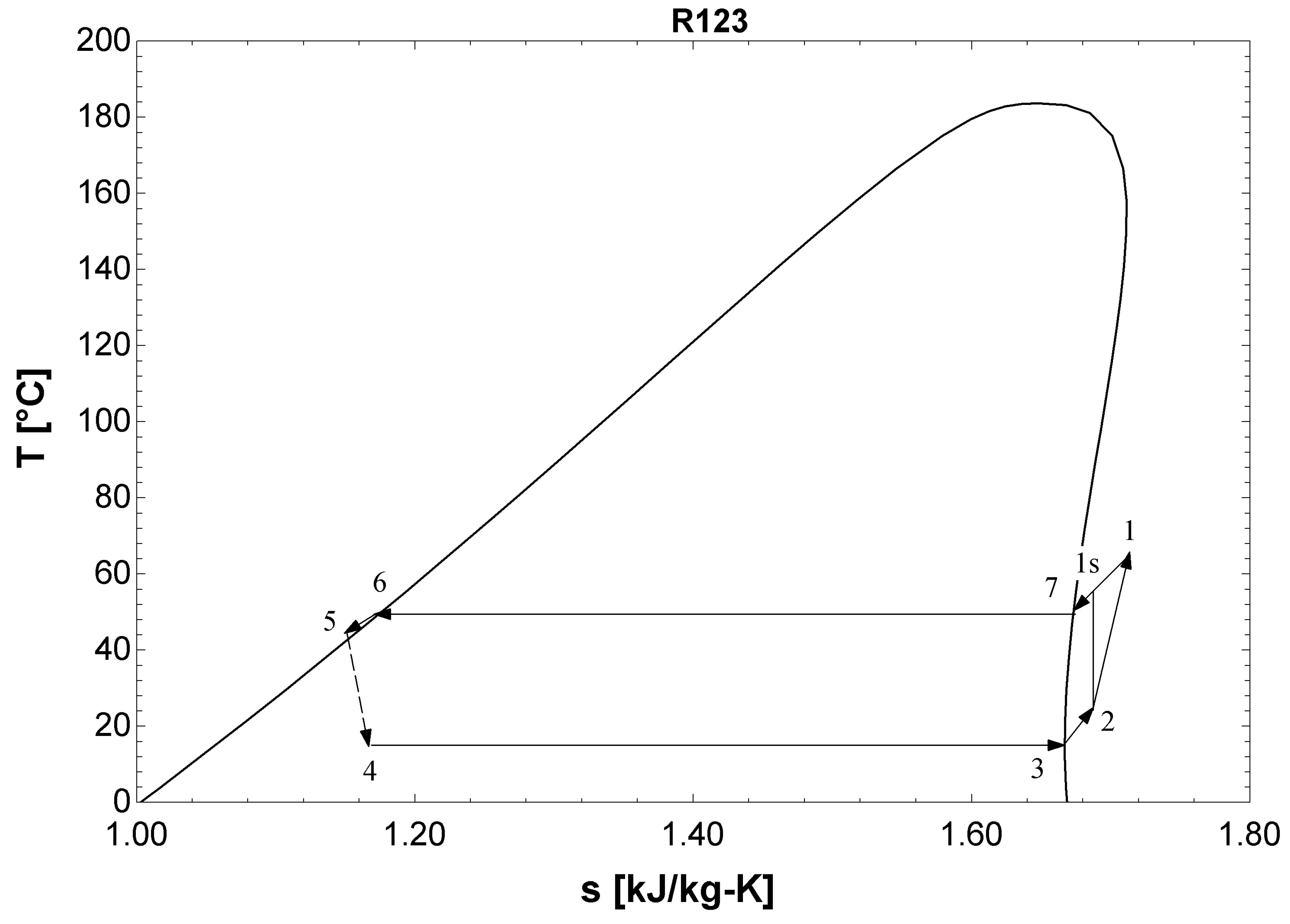
Figure A1 shows the Temperature entropy (T–S) diagram of the heat pump system.
Figure A1. Temperature entropy diagram of heat pump system (working fluid: R123).
Processes 10 00121 g0a1
In this system, the heat exchange rate of evaporator is
Q eva = m hp ( h 2 - h 4 ) = 4 . 2 m hw ( T hw , in - T hw , out )
where m hp is the mass flow rate of heat pump, kg/s; h 2 is the outlet enthalpy of evaporator, kJ/kg; h 4 is the inlet enthalpy of evaporator, kJ/kg; m hw is the mass flow rate of hot water (mass flow of geothermal water), kg/s; T hw , in is the inlet temperature of hot water, K; T hw , out is the outlet temperature of hot water, K; Q eva is the heat exchange rate of evaporator, kW.
The heat exchange rate of condenser is
Q con = m hp ( h 1 - h 5 ) = 4 . 2 m cw ( T cw , in - T cw , out )
where h 1 is the inlet enthalpy of condenser, kJ/kg; h 5 is the outlet enthalpy of condenser, kJ/kg; m cw is the mass flow rate of cooling water, kg/s; T cw , in is the inlet temperature of cooling water, K; T cw , out is the outlet temperature of cooling water, K; Q con is the heat exchange rate of condenser, kW.
The isentropic efficiency of the working fluid pump is 0.76. Theoretically, the compression process of the working fluid is an isentropic process (process 2-1s). However, the real process is irreversible (process 2-1). The isentropic efficiency of the working fluid pump is:
η is = (   h 1 s - h 2 )   /   ( h 1 -   h 2 )
where h 1 s is the outlet enthalpy of working fluid pump in theory, kJ/kg; η is is the isentropic efficiency of the working fluid pump, %.
The Energy consumption of working fluid pump is:
W hp , pump = m h p ( h 1 - h 2 ) / η
where W hp , pump is the energy consumption of working fluid pump, kW; η is the efficiency of working fluid pump, %.
The coefficient of performance (COP) of the heat pump is:
COP = Q con /   W hp , pump

References

  1. Gallup, D.L. Production engineering in geothermal technology: A review. Geothermics 2009, 38, 326–334. [Google Scholar] [CrossRef]
  2. Aghahosseini, A.; Breyer, C. From hot rock to useful energy: A global estimate of enhanced geothermal systems potential. Appl. Energy 2020, 279, 115769. [Google Scholar] [CrossRef]
  3. Olasolo, P.; Juárez, M.C.; Morales, M.P. Enhanced geothermal systems (EGS): A review. Renew. Sustain. Energy Rev. 2016, 56, 133–144. [Google Scholar] [CrossRef]
  4. Breede, K.; Dzebisashvili, K.; Liu, X.; Falcone, G. A systematic review of enhanced (or engineered) geothermal systems: Past, present and future. Geotherm. Energy 2013, 1, 1–27. [Google Scholar] [CrossRef] [Green Version]
  5. Wang, X.X.; Wu, N.Y.; Su, Z.; Zeng, Y.C. Progress of the enhanced geothermal systems (EGS) development technology. Prog. Geophys. 2012, 27, 355–362. [Google Scholar]
  6. Rybach, L.; Hopkirk, R.J. Shallow and deep borehole heat exchangers—Achievements and prospects. In Process World Geothermal Congress; International Geothermal Association: Florence, Italy, 1995; pp. 2133–2138. [Google Scholar]
  7. Dijkshoorn, L.; Speer, S.; Pechnig, R. Measurements and Design Calculations for a Deep Coaxial Borehole Heat Exchanger in Aachen, Germany. Int. J. Geophys. 2013, 2013, 14. [Google Scholar] [CrossRef]
  8. Sapinskasliwa, A.; Rosen, M.A.; Gonet, A.; Sliwa, T. Deep Borehole Heat Exchangers—A Conceptual and Comparative Review. Int. J. Air Cond. Refrig. 2015, 24, 1630001. [Google Scholar] [CrossRef]
  9. Cai, W.L.; Wang, F.H.; Liu, J.; Wang, Z.; Ma, Z. Experimental and numerical investigation of heat transfer performance and sustainability of deep borehole heat exchangers coupled with ground source heat pump systems. Appl. Therm. Eng. 2019, 149, 975–986. [Google Scholar] [CrossRef]
  10. Wang, Z.; Wang, F.H.; Liu, J.; Ma, Z.; Han, E.; Song, M. Field test and numerical investigation on the heat transfer characteristics and optimal design of the heat exchangers of a deep borehole ground source heat pump system. Energy Convers. Manag. 2017, 153, 603–615. [Google Scholar] [CrossRef]
  11. Li, C.; Guan, Y.; Yang, R.; Lu, X.; Xiong, W.; Long, A. Effect of inner pipe type on the heat transfer performance of deep-buried coaxial double-pipe heat exchangers. Renew. Energy 2019, 145, 1049–1060. [Google Scholar] [CrossRef]
  12. Ali, M.A.M.; El-Maghlany, W.M.; Eldrainy, Y.A.; Attia, A. Heat transfer enhancement of double pipe heat exchanger using rotating of variable eccentricity inner pipe. Alex. Eng. J. 2018, 57, 3709–3725. [Google Scholar] [CrossRef]
  13. Mokhtari, H.; Hadiannasab, H.; Mostafavi, M.; Ahmadibeni, A.; Shahriari, B. Determination of optimum geothermal Rankine cycle parameters utilizing coaxial heat exchanger. Energy 2016, 102, 260–275. [Google Scholar] [CrossRef]
  14. Iry, S.; Rafee, R. Transient numerical simulation of the coaxial borehole heat exchanger with the different diameters ratio. Geothermics 2018, 77, 158–165. [Google Scholar] [CrossRef]
  15. Oh, K.; Lee, S.; Park, S.; Han, S.I.; Choi, H. Field experiment on heat exchange performance of various coaxial-type ground heat exchangers considering construction conditions. Renew. Energy 2017, 144, 84–96. [Google Scholar] [CrossRef]
  16. He, Y.; Bu, X.B. A novel enhanced deep borehole heat exchanger for building heating. Appl. Therm. Eng. 2020, 178, 115643. [Google Scholar] [CrossRef]
  17. Fang, L.; Diao, N.; Shao, Z.; Zhu, K.; Fang, Z. A computationally efficient numerical model for heat transfer simulation of deep borehole heat exchangers. Energy Build. 2018, 167, 79–88. [Google Scholar] [CrossRef]
  18. Naldi, C.; Zanchini, E. A new numerical method to determine isothermal g-functions of borehole heat exchanger fields. Geothermics 2019, 77, 278–287. [Google Scholar] [CrossRef]
  19. Song, X.; Wang, G.; Shi, Y.; Li, R.; Xu, Z.; Zheng, R.; Wang, Y.; Li, J. Numerical Analysis of Heat Extraction Performance of a Deep Coaxial Borehole Heat Exchanger Geothermal System. Energy 2018, 164, 1298–1310. [Google Scholar] [CrossRef]
  20. Luo, Y.; Yu, J.; Yan, T.; Zhang, L.; Liu, X. Improved analytical modeling and system performance evaluation of deep coaxial borehole heat exchanger with segmented finite cylinder-source method. Energy Build. 2020, 212, 109829. [Google Scholar] [CrossRef]
  21. Beier, R.A. Thermal response tests on deep borehole heat exchangers with geothermal gradient—Science Direct. Appl. Therm. Eng. 2020, 178, 115447. [Google Scholar] [CrossRef]
  22. Li, J.; Xu, W.; Li, J.; Huang, S.; Li, Z.; Qiao, B.; Yang, C.; Sun, D.; Zhang, G. Heat extraction model and characteristics of coaxial deep borehole heat exchanger. Renew. Energy 2021, 169, 738–751. [Google Scholar] [CrossRef]
  23. Daneshipour, M.; Rafee, R. Nanofluids as the circuit fluids of the geothermal borehole heat exchangers. Int. Commun. Heat Mass Transf. 2017, 81, 34–41. [Google Scholar] [CrossRef]
  24. Bu, X.; Jiang, K.; Li, H. Performance of geothermal single well for intermittent heating. Energy 2019, 186, 115858. [Google Scholar] [CrossRef]
  25. Bär, K.; Rühaak, W.; Welsch, B.; Schulte, D.; Homuth, S.; Sass, I. Seasonal high temperature heat storage with medium deep borehole heat exchangers. Energy Procedia 2015, 76, 351–360. [Google Scholar] [CrossRef] [Green Version]
  26. Welsch, B.; Ruehaak, W.; Schulte, D.O.; Baer, K.; Sass, I. Characteristics of medium deep borehole thermal energy storage. Int. J. Energy Res. 2016, 40, 1855–1868. [Google Scholar] [CrossRef]
Figure 1. Diagram of the DBHE system.
Processes 10 00121 g001
Figure 2. (a) Outlet temperature from the simulation; (b) experimental outlet temperature [9]. (Reproduced with permission from Wang, Applied Thermal Engineering; published by Elsevier, 2019).
Processes 10 00121 g002
Figure 3. (a) Outlet temperatures of Mode 1, (b) Mode 2, and (c) Mode 3.
Processes 10 00121 g003aProcesses 10 00121 g003b
Figure 4. Heat extraction rates from wells.
Processes 10 00121 g004
Figure 5. Heat extraction rates from the condenser of the heat pump system.
Processes 10 00121 g005
Figure 6. Rock temperature at different depths for Mode 1.
Processes 10 00121 g006
Figure 7. Rock temperature comparison for three modes.
Processes 10 00121 g007
Figure 8. Rock temperature recover at 1998 m for Mode 1.
Processes 10 00121 g008
Figure 9. Rock temperature recover at 1000 m for Mode 1.
Processes 10 00121 g009
Table 1. The parameters of demonstration project [9] (Reproduced with permission from Wang, Applied Thermal Engineering; published by Elsevier, 2019).
Rock Soil AreaDepth (m)Density (kg/m3)Specific Heat Capacity (J/kg·K)Thermal Conductivity (W/m·K)
10–500176014331.59
2500–720186010251.65
3720–145020708781.76
41540–200022708481.88
Table 2. The parameters of the DBHE [9] (Reproduced with permission from Wang, Applied Thermal Engineering; published by Elsevier, 2019).
Size
(mm)
Length (m)Density (kg/m3)Specific Heat Capacity (J/kg·K)Thermal Conductivity (W/m·K)
Inner pipe (HDPE)Φ110 × 10199895023000.45
Outer pipe (Seamless steel J55)Φ177.8 × 9.192000785049840
Table 3. The parameters of the heat pump system.
ParameterValueParameterValue
Evaporation temperature50 °CSuperheat of evaporator10
Condensation temperature15 °CSupercool of condenser5
Working fluid pump efficiency60%
Table 4. Peak and valley electricity prices in China.
TimeUnit Price (USD/(kW·h))
8:00–11:00, 18:00–23:000.21
7:00–8:00, 11:00–18:000.18
23:00–7:000.07
Table 5. Outlet temperatures of Modes 1, 2, and 3.
Mass Flow (kg/s)
13579
Outlet temperature (°C)Mode 150.1233.5428.6826.3825.05
Mode 264.0242.3434.1630.2828.06
Mode 363.0542.4134.0030.2727.75
Table 6. Energy consumption of the working fluid pump in the heat pump system.
Mass Flow (kg/s)
13579
Energy consumption (kW)Mode 137.0049.8953.3154.8655.83
Mode 254.0782.3286.9688.3989.10
Mode 352.8882.5885.9888.3085.67
Table 7. The electricity charge for the heat pump system running for one day in each mode.
Mass Flow (kg/s)
13579
Total price (USD)Mode 1136.2183.6196.2201.9205.5
Mode 281.1123.5130.4132.6133.7
Mode 352.982.686.088.385.7
Table 8. Monthly temperature recovery of rock.
Temperature (°C)
Time (Month)Mode 1Mode 2Mode 3
028.5551.9543.25
169.1572.4571.25
272.5574.8574.05
374.2575.9575.35
475.3576.6576.25
576.0577.1576.75
676.5577.5577.15
776.9577.8577.45
877.2578.0577.75
Publisher’s Note: MDPI stays neutral with regard to jurisdictional claims in published maps and institutional affiliations.

