Abstract
Joint pain is a prominent symptom of Hip and Knee Osteoarthritis (OA), impairing patients’ movements and affecting the joint mechanics of walking. Self-report questionnaires are currently the gold standard for Hip OA and Knee OA pain assessment, presenting several problems, including the fact that older individuals often fail to provide accurate self-pain reports. Passive methods to assess pain are desirable. This study aims to explore the feasibility of OA-Pain-Sense, a passive, automatic Machine Learning-based approach that predicts patients’ self-reported pain levels using SpatioTemporal Gait features extracted from the accelerometer signal gathered from an anterior-posterior wearable sensor. To mitigate inter-subject variability, we investigated two types of data rescaling: subject-level and dataset-level. We explored six different binary machine learning classification models for discriminating pain in patients with Hip OA or Knee OA from healthy controls. In rigorous evaluation, OA-Pain-Sense achieved an average accuracy of 86.79% using the Decision Tree and 83.57% using Support Vector Machine classifiers for distinguishing Hip OA and Knee OA patients from healthy subjects, respectively. Our results demonstrate that OA-Pain-Sense is feasible, paving the way for the development of a pain assessment algorithm that can support clinical decision-making and be used on any wearable device, such as smartphones.
1. Introduction
Motivation: Osteoarthritis (OA) is a progressive joint ailment that leads to weight-bearing joint dysfunction and pain, limits patient mobility and quality of life, and causes an enormous economic burden [1,2,3,4]. Nearly 500 million individuals are affected by OA worldwide, and a third of the population is expected to experience OA by 2030 [5,6]. Hip and Knee Osteoarthritis (HKOA) are the most prevalent types of OA in the United States (US) and worldwide, afflicting 12% of the world’s population [7,8], and 32.5 million adults in the US [6]. OA primarily affects middle-aged to older adults and ranks 12th out of 359 conditions contributing to global disability [7]. In 2020, there were roughly 650 million individuals with knee OA (KOA) globally, and 7–25% of people ages 56 and older have Hip OA (HOA) [9,10]. Figure 1 shows the trajectory of past OA diagnoses as well as future projections of 100 types of arthritis, with OA being the most common type [11].
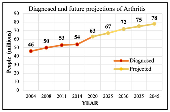
Figure 1.
The diagnosed and projected Arthritis.
The OA problem: Pain is a common clinical characteristic of OA, and the hallmark complaint and manifestation of incapacitation of HKOA patients, impacting sleep, mood, and mobility [10,12,13]. OA pain is caused by the stretching of tendons and ligaments after the surface cartilage has worn away, causing bones to rub against each other painfully and compromising the patient’s movement [14]. Figure 2 illustrates the differences between a hip with OA and a healthy hip and between a knee with OA and a healthy knee. OA pain is unequally distributed and drives patients to seek healthcare intervention, resulting in rising medical costs [13,15]. Periodic OA pain assessment is necessary to guide treatment. However, in clinical practice, pain assessment is currently conducted using self-report questionnaires and physical examination [16]. The Western Ontario and McMaster Universities Osteoarthritis Index (WOMAC) is the most widely used self-administered instrument for assessing pain, physical activity, and stiffness in HKOA patients. The Hip disability and Osteoarthritis Outcome Score (HOOS), Knee Injury and Osteoarthritis Outcome Score (KOOS), and other self-administered hip-specific and knee-specific questionnaires were developed from the WOMAC for younger and elderly patients with end-stage OA. Therefore, in this study, we utilize patients’ self-reported HOOS and KOOS scores since they are reliable and responsive instruments for HKOA patients involving those eligible for total hip/knee replacement surgery [17,18]. These questionnaires assess pain comprehensively, containing separate subscales that assess various aspects, including patient’s pain, symptoms, activities of daily living for physical function, sport and recreation function, and hip/knee-related quality of life. The overall pain subscale scores are scaled from 0 to 100, where 100 represents no pain and 0 represents severe pain.

Figure 2.
Anatomy of (A) Hip Osteoarthritis vs. Normal Hip (Reproduced with permission from OrthoInfo. © American Academy of Orthopaedic Surgeons. https://orthoinfo.org/ accessed on 26 March 2022) [19], (B) Knee Osteoarthritis vs. Normal Knee (rights in the images are owned by a third party) [20].
The need for objective OA pain assessment methods: Several problems arise with self-report questionnaires, including the fact that patient responses are influenced by psychological and sociocultural factors such as catastrophizing. These factors introduce bias. Sociocultural factors often rely on interpretation by a physician’s subjective judgment, which increases the risk of erroneous or biased assessments [13,21]. Older individuals fail to provide accurate self-pain reports because they are afraid of hospitalization, medications, and expenses [22]. The consequence of failure to adequately assess self-reported HKOA pain inevitably leads to inappropriate clinical decision-making in pain management. In addition to the above-mentioned limitations of pain assessment methods, OA patients with the same OA stage severity have been found to experience varying levels of pain [13]. Thus, developing an algorithm that estimates the patient’s self-reported HOOS/KOOS scores and predicts their pain level more accurately and consistently is a crucial task, especially if it can be integrated into the clinical system. Such an algorithm would make a patient’s accurate pain level available to the physician in a way that contributes to timely and appropriate interventions and assists in targeting the right treatments.
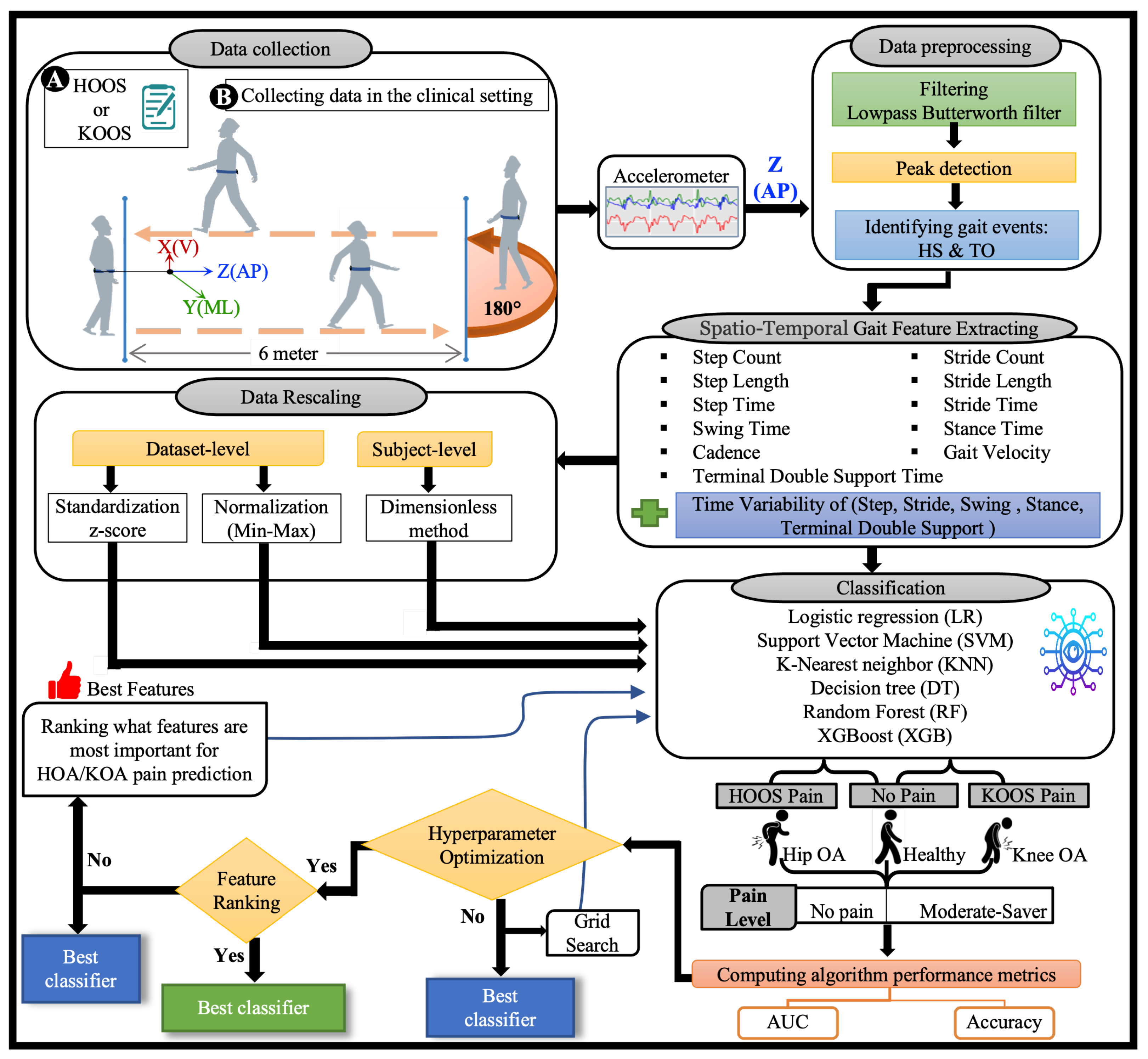
Our OA-Pain-Sense approach: In this paper, we investigate the feasibility of OA-Pain-Sense, a machine learning-based system that can be effectively and reliably employed to intelligently and consistently assess and report HKOA patients’ HOOS/KOOS pain scores in a clinical setting. OA-Pain-Sense analyzes accelerometry data from a lumbar-mounted Inertial Measurement Unit (IMU) sensor and estimates clinical characteristics of gait (walk). Gait is one of the physical functions compromised by pain in HKOA patients [23]. Late-stage HKOA patients experience frequent pain and discomfort when walking or moving the joint due to the friction between the moving parts of a joint [24]. OA-Pain-Sense is the first attempt toward validating SpatioTemporal Gait Parameters (STGPs) as features that are then classified using Machine Learning (ML) algorithms in order to predict the HOOS/KOOS pain levels reported by end-stage HKOA patients from the Anterior-Posterior (AP) accelerometer signals. We believe ML could provide a new approach for developing a pain assessment tool to predict pain levels by combining multiple STGPs in a single ML model.
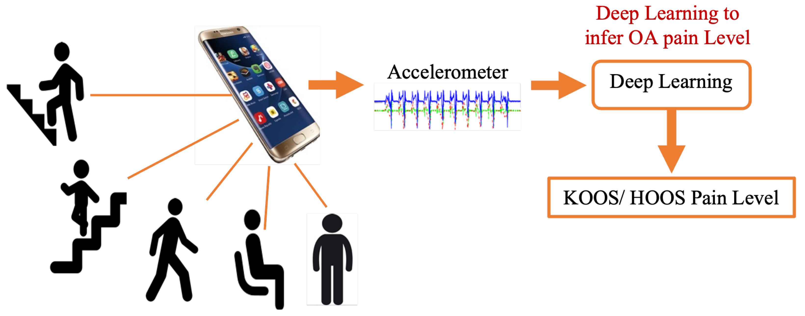
However, several questions arise about this approach’s feasibility, accuracy, and reliability, which are explored in this paper. Specifically, this work focuses on determining the most important STGPs that can be used as input features to a traditional machine learning classifier algorithm to differentiate between HOOS/KOOS moderate–severe pain and no pain in HKOA patients as a step toward developing the OA-Pain-Sense framework. A key feature of this proposed framework is employing only a single-axis accelerometer signal in the AP direction along with investigating the best data rescaling methods to achieve high classification performance [25,26,27,28]. The use case utilized in this paper involves active involvement of the patient and focuses on validating the ML prediction from STGP features. The patient would wear the IMU sensor on their lumbar region and walk. IMU sensor data would be gathered and transmitted to the OA Sense ML pain prediction module in the cloud, which would predict and send back the patient’s pain level back to their provider. Our eventual OA-Pain-Sense use case illustrated in Figure 3 is a more ambitious passive, continuous use case that presents the patient with minimal burden. Accelerometer sensor data would be gathered passively from the sensors built into the patient’s smartphone as they live their lives. The accelerometer data could be analyzed by the cloud-based ML pain prediction method to generate frequent, consistent, and objective feedback that would engage patients more in their care. We chose a lumbar-mounted IMU placement as the first step toward real-world scenarios that utilize smartphones for data gathering in free-living scenarios as people usually carry their phones in their front or back trouser pockets. Figure 4 depicts our OA-Pain-Sense system pipeline.
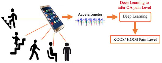
Figure 3.
OA-Pain-Sense future application.
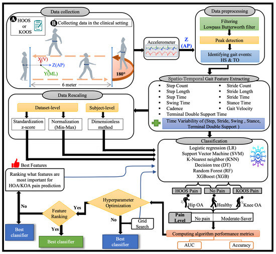
Figure 4.
The OA-Pain-Sense framework shows four different experimental datasets used as input to the classification models. The data collection block shows the IMU location on a subject’s lower back for the 2 min walk trails. The raw accelerometer signal in the Anterior-Posterior (AP) direction is input into the data pre-processing block to filter and detect heel strikes and toe-off events. The STGPs are computed after the pre-processing step and fed to the ML classification algorithms (first dataset). STGPs are passed to the data rescaling block to apply dataset-level (two methods: z-score and min-max) and subject-level (one method: dimensionless) normalization and then fed to ML algorithms.
Challenges: Predicting self-report pain levels based on STGPs is a challenging technical problem for the following reasons:
- 1.
- IMU accelerometer signals are usually noisy and have some bias in the data.
- 2.
- STGP features extracted from IMU data may be affected by variations in a patient’s self-selected pace, which may vary substantially over the data collection period.
- 3.
- Distinct gait events such as heel strike and the start/stop of each step within the accelerometer signal may be challenging to distinguish as there can be multiple such events in a single step, leading to an incorrect count of the number of steps and, in turn, the wrong measurement of the STGPs.
- 4.
- Machine Learning models may be affected by the variability in the subject’s gait and dispersion of the raw gait data, which leads to a lack of ML model generalizability.
Background: STGPs are the most common gait parameters extracted and used for gait measurements. STGPs include gait velocity (walking speed), cadence, step time, stride time, stance time, swing time, double support time, step length, and stride length [29,30]. STGPs can be affected by walking-induced pain in HKOA patients [31,32]. STGP assessment is of particular importance in clinical practice and provides information on relevant and functional aspects of patient’s suffering, and therefore reflects HKOA patients’ pain manifested through their gait dysfunction [33,34,35]. Prior research has demonstrated promising results of using STGPs in classifying individuals with gait disorders as a marker of an increased risk of incidents of various conditions, including stroke, depression, and Parkinson’s disease [36,37,38,39,40]. Accordingly, in this study, we employed the STGPs to predict the self-reported pain of HKOA patients.
In clinical settings, STGPs are currently often extracted from clinical gait lab data acquired from the patients while they are performing a clinical walking test. Such clinical data collection utilizes instrumented walkways or motion-capture systems [41]. Although extracting STGP from gait lab data is a gold standard, it is tedious, time-consuming, and expensive as it requires a lengthy calibration process and the involvement of qualified experts. Furthermore, it involves a cumbersome, intrusive marker setup process and restricts the patient’s typical movement. Moreover, waiting lists for such gait analyses can be long, and the patient may remain on a waiting list for an unspecified period. Finally, a clinical gait lab is costly, not portable, and not always accessible to many patients [42,43,44].
Wearable technologies have become vital measuring instruments that can provide an efficient measurement of STGPs [45], including outside the clinic, possibly decreasing the demand for clinicians’ time. In the literature, the Inertial Measurement Unit (IMU) sensor is one of the most frequently used wearable technologies for measuring STGPs. The IMU incorporates a tri-axis accelerometer and tri-axis gyroscope that can be used to capture various valuable and accurate gait parameters, gait-related outcomes [46,47], and rich information about gait abnormalities [48,49,50]. Moreover, IMUs are affordable, portable, and can be used outside laboratory environments [44].
In recent years, extracting STGP features from data captured from IMU sensors attached to a subject’s body has become indispensable in HKOA research studies [51,52,53,54,55]. In the literature, signals captured from multiple IMU placed on various body parts have been used to compute STGPs in HKOA patients [54,55,56,57,58]. However, as the trunk is mostly stable, during locomotion, a single IMU attached to the lumbar spine/lower back provides the most reliable information of all body parts [25,26]. Figure 5 shows the lower back on the spine area.
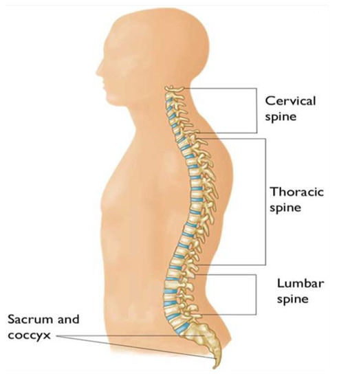
Figure 5.
The regions of the spine, including the lumbar spine (Reproduced with permission from OrthoInfo. © American Academy of Orthopaedic Surgeons. https://orthoinfo.org/ accessed on 20 February 2022).
The AP accelerometer signal of IMU has been found to be the most revealing signal in identifying valid gait cycle events in prior work, mainly in research involving pathological subjects [59,60,61,62]. Specific gait cycle events are then detected and used to facilitate reliable STGP measurements [63,64]. Many research studies have proven the effectiveness of utilizing AP accelerometer signals in determining important gait events that are necessary to compute STGPs. However, there is a lack of research extracting the STGPs based solely on AP accelerometer signals in the HKOA population. We believe that measuring STGPs for HKOA patients using the AP axis/direction of the acceleration signal is novel and of interest to the OA community, especially if these STGPs are employed to assess if an HKOA patient is suffering from pain or not.
Mean STGPs have been highlighted as sensable biomechanical parameters that discriminate severe OA patients with end-stage OA) from healthy control groups [65,66]. Many OA research studies have utilized the mean of STGPs as primary outcomes derived from IMU sensors placed on patients’ lower backs because the mean of STGPs is a reliable and practical method for estimating the gait of end-state HKOA patients. Hence, the mean of STGPs can be utilized for predicting the pain level of HKOA patients, facilitating reliable pain assessment that clinicians can use to improve the quality of care.
ML has successfully been used for various OA and medical applications in general and to predict HKOA pain in particular [67,68]. Many different ML-based methods for predicting the pain levels of HKOA patients have been proposed [69,70,71]. However, less attention has been paid to directly classify STGPs as input features for ML algorithms in order to predict the pain level of HKOA patients. Consequently, in this research, we build ML models to predict the pain of HKOA patients using STGP features, filling a critical gap in the literature.
To the best of our knowledge, no prior work has proposed a comprehensive, cost-effective, ML-based framework to predict HKOA self-report patients’ pain using data from objective wearable IMU sensors by extracting STGP features from a single-direction accelerometer signal. This work fills that gap by performing binary ML classification of pain (Yes/No) in HKOA patients using STGP features. As many widely owned smartphones are equipped with the necessary IMUs for data collection, we envision that in the future, smartphones can be used for predicting patients’ HOOS/KOOS pain levels using ML based on STGP features without any human intervention.
Our contributions: include
- 1.
- A complete ML HKOA pain prediction pipeline of steps for OA-Pain-Sense, as depicted in Figure 4, comprises six main steps: signal pre-processing (filtering and gait event detection), STGP feature extraction, feature rescaling, model hyperparameter optimization, feature ranking, and classification.
- 2.
- Pre-processing steps are designed to mitigate noisy IMU sensor data and improve results. These steps include fourth order low-pass Butterworth filtering of the AP Acceleration signal (AccAP) and identification of Heel Strike (HS) and Toe-Off (TO) gait events in the filtered AccAP signal that facilitate segmentation of the continuous AccAP signal.
- 3.
- Extraction of a comprehensive set of STGP features motivated by prior work. After segmenting the filtered AccAP data into gait cycles, twenty-one (eleven STGPs, five Time Variability (Var), and five Fluctuation Magnitude (FM) for temporal gait) features were computed.
- 4.
- ML learning classification of the extracted STGP features, and trained and tested six ML classification algorithms to predict subjects’ HOOS/KOOS moderate-to-severe pain (<100 HOOS/KOOS pain score) from no-pain (binary classification): Logistic Regression (LR), Support Vector Machines (SVM), K-Nearest Neighbours (KNN), Decision Tree (DT), Random Forest (RF), and XGBoost (XGB).
- 5.
- Investigation of the effectiveness of two types of signal data rescaling in mitigating variability in the data: subject-level normalization applied in STGPs using a Dimensionless (DL) method and dataset-level normalization of the STGP data. The DL normalization method employed corrections for anthropometric variations between the subjects. Application of the rescaling methods yielded four experimental datasets: STGP, normalized STGP (STGP-Normz), standardized STGP (STGP-Standz), and dimensionless STGP (DL STGP), which were utilized for training and testing six ML pain classification algorithms.
- 6.
- A comprehensive evaluation of the proposed pain prediction methods using 5-fold cross-validation on data from 51 HKOA patients and 27 age-matched healthy controls (HC) with subject-level splitting to avoid data leakage.
Summary of our findings: An LR classifier trained on DL STGP achieved an optimal classification mean accuracy of 84.91% for HOA vs. HC and presented the highest mean accuracy (80.73%) using STGP-Standz for KOA vs. HC. To further optimize the performance of our model, hyperparameter tuning was conducted using grid search, enabling us to achieve 86.79% by DT using STGP-Norm data and 83.57% by SVM using STGP-Normz data for HOA vs. HC and KOH vs. HC, respectively. Finally, feature ranking was carried out according to feature importance values generated by the RF algorithm. We found that gait velocity, cadence, step count, stride count, step time, stride time, step length, and stride length were the most important features for classifying both HOA vs. HC and KOA vs. HC. We investigated classification using the top 1, 3, 5, and 10 features. However, we noticed that reducing the number of features also utilized the reduced RF model’s performance. However, utilizing SVM with the top three features for classifying HOA vs. HC, we achieved a similar accuracy using all features. For classifying KOA vs. HC, using the top five features with KNN, we achieved close to the accuracy when all features were utilized.
2. Related Work
2.1. Wearable Sensor-Based Gait Parameter Extraction
Several studies have utilized various analytical approaches for analyzing gait parameters, including statistical significance assessment tests such as the t-test and the Analysis Of Variance (ANOVA). A study by [53] investigated the effects of walking speed differences on the STGP in end-stage HOA patients vs. HC based on normal and matched speed using Statistical Parametric Mapping (SPM) analysis. They found that HOA patients had a significantly slower walking speed with a lower cadence and a shorter single support phase (p-value < 0.001) than HC. Christian et al. [25] analyzed gait variability and symmetry in KOA patients based on AP axis data obtained from a tri-axial accelerometer positioned on the patient’s lower back. They computed the mean step and stride times to determine stride and step regularity and symmetry. KOA patients were found to have significantly greater mean stride times and step times than healthy control, while both groups had statistically insignificant stride and step time variability. Bolink et al. [26] defined physical function parameters such as walk speed, cadence, step time, and step length that can discriminate patients with severe stage KOA from healthy controls. Their results indicate statistically significant differences in the walking speed, cadence, step length (p-value < 0.001), and step time (p-value < 0.05) of KOA patients in comparison to HC. A study from [61] computed the mean step time and mean stride time from a 9 min walk data, comparing older patients with bilateral KOA and age-matched HC group according to sex. Andrade et al. [72] presented significant differences (p < 0.05) between the mean step and stride times of patients with unilateral HOA and healthy controls. The inertial sensor system RehaGait® was employed by [73] to distinguish STGPs between the affected and unaffected side in unilateral KOA patients and between end-stage KOA patients and healthy control subjects. Their results indicated that the gait velocity was slow, the stride duration was longer, and the cadence was lower in KOA patients (p < 0.001). In the [74] study, mean walking velocity, mean stride length, and mean cadence were computed to discover statistically significant differences between young (age 21–35) and older (age 65–80) asymptomatic and KOA patients. Table 1 summarizes prior work using mean STGP in HKOA studies.

Table 1.
Mean STGP features prior to HKOA studies have found statistically significant differences in HKOA patients vs. healthy controls.
2.2. Machine Learning-Based Prediction of Pain
In comparison to statistical analysis methods that often establish relationships between individual STGPs and a patient’s pain, ML methods are more accurate because they explore relationships with combinations of multiple STGPs. Developing ML prediction models for various prediction tasks in OA applications has been reported in the literature using MRI, X-ray, clinical information, and biomechanical data as inputs to ML models [76,77,78,79]. However, in this review, we focus on ML models to predict pain related to OA, which have mostly focused on predicting pain related to KOA. In fact, to the best of our knowledge, only one study in the literature focused on predicting pain in HOA patients. A study by [71] applied an ML approach to predict HOA patients’ pain levels during a five min walk based on Electroencephalography (EEG) features. They achieved 79.6% accuracy using the SVM algorithm. However, EEG studies need to be conducted in a laboratory or specialized clinics, are expensive, and can be problematic for translation to large-scale clinical practice. Alexos et al. [70] used ML to predict pain in KOA patients based on the WOMAC pain progression data extracted from the Osteoarthritis Initiative (OAI) database—“a multicenter, observational study of knee OA containing 4796 subjects conducted in the United States”—showed the ability of ML to classify pain progression condition: pain decline, no significant pain change, and pain increase, achieving 84.3% and 82.5% accuracy for the prediction of pain on the left leg and the right leg, respectively, using an RF classifier. Marieke et al. [80] also developed an ML model to predict Frequent Knee Pain (FKP) and symptomatic KOA in overweight and obese middle-aged women based on questionnaire and physical examination variables. They achieved an Area Under the Curve (AUC) of 71% for predicting FKP. This study utilized Multivariable analysis by backward stepwise deletion. Deep learning and traditional ML algorithms were also utilized to analyze knee radiographs by [69] in order to predict pain progression in patients with KOA. The authors reported that their Artificial Neural Network (ANN) and Convolutional Neural Network (CNN) models achieved AUCs of 69.2% and 77%, respectively. The drawbacks of prior studies are that they predominantly utilized data collected in the clinic or required patient–clinician encounters and controlled laboratory settings, which have a high cost in terms of money and time. Therefore, there is a need to develop assessment methods that can be utilized in real-life environments, such as the patient’s home, and can report patients’ pain at an affordable price, minimize in-person clinical visits, and predict patients’ self-reported pain objectively rather than subjectively.
3. Materials and Methods
3.1. Data Acquisition
3.1.1. Participants and Clinical Assessment
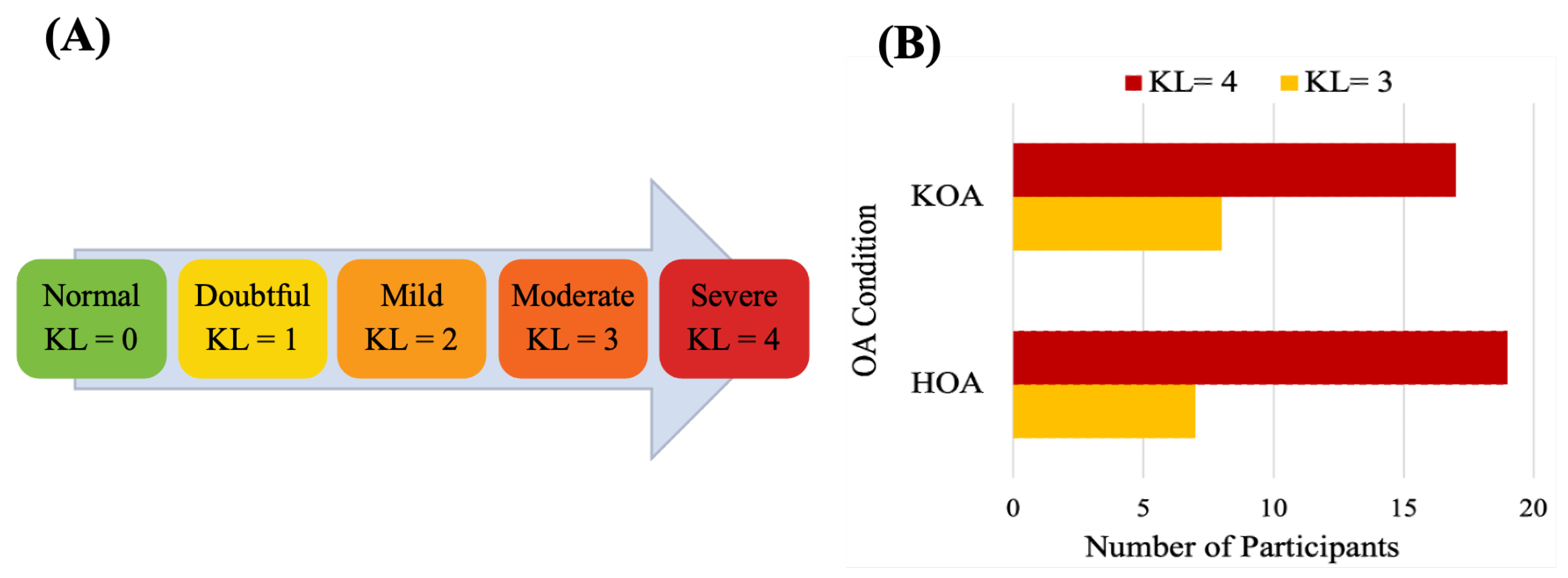
The data used in this study were collected at the Sint Maartenskliniek, Netherlands [81]. Fifty-three patients with unilateral end-stage hip (n = 26 ) or knee (n = 25) OA and 27 HC in the same age range were recruited. The OA group was included based on the following criteria: Body Mass Index (BMI) ≤ 40 kg/m, had radiological and symptomatic OA, waiting for joint replacement surgery, able to walk more than 2 min without any assistive device, no other musculoskeletal or neurological affecting gait or balance and no joint replacement within a year in another weight-bearing joint. Subjects for the healthy control group met all the same criteria, except radiographic evidence of hip or knee OA and no history of any pain in the lower back. The HKOA severity is assessed by experienced orthopedic surgeons based on the Kellgren–Lawrence (KL) radiographic severity scale, the radiographic metric commonly used to measure OA progression [82]. Reference values for KL grading scale [83] and the statistical distributions of KL scores of HKOA patients in our dataset are shown in Figure 6. Patients with OA completed the HOOS or KOOS to assess self-reported functioning [17,18]. Table 2 presents the list of HOOS and KOOS pain-related questions. Patients’ overall HOOS/KOOS scores were used as ML prediction target variables. Table 3 summarizes the demographic and clinical attributes of the study participants.

Figure 6.
(A) Kellgren–Lawrence grading scale and (B) statistical distributions of Kellgren–Lawrence scores of HOA and KOA patients.

Table 2.
The HOOS and KOOS subscales pain items.

Table 3.
Demographic data and clinical information of the study participants.
3.1.2. Instruments and Protocol
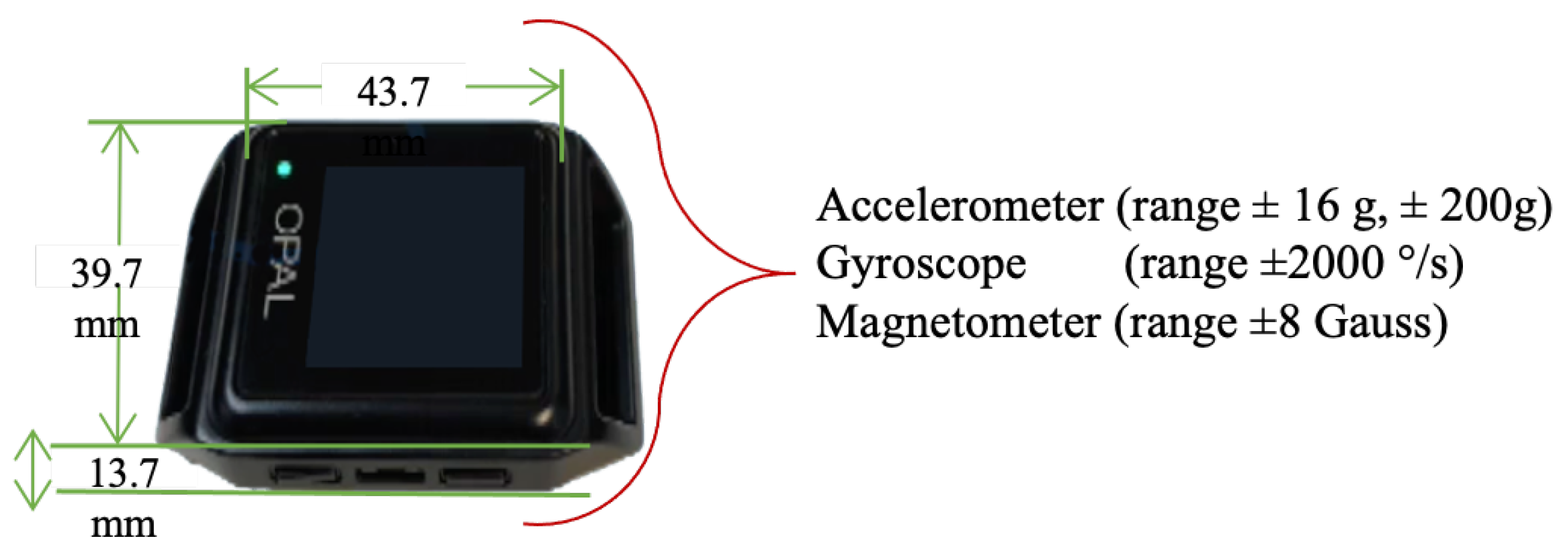
Gait data were collected using four wearable wireless IMUs (APDM Opal V2, APDM Inc., Portland, OR, USA. Sensors were attached to the subjects’ sternum, dorsum of both feet, and lumbar using elastic straps. The APDM Opal is a wristwatch-sized device that provides tri-axial accelerometer, gyroscope, and magnetometer data at a sampling rate of 128 Hz [84,85]. The IMU Opal V2 Characteristics are shown in Figure 7. Data were collected while participants walked across a 6 m walkway incorporating a 180 turn at a self-selected preferred pace for 2 min, barefoot or wearing comfortable flat shoes as shown in Figure 4 (data collection box).

Figure 7.
APDM Opal V2 IMU.
3.2. Data Preprocessing
In this work, all data processing and implementation of the rest of OA-Pain-Sense were conducted using the Python language version 3.9.5 in Visual Studio Code version 1.59.0. The data used in this study were extracted from a lumbar-mounted IMU in order to mimic a common smartphone placement (e.g., in the hip pocket or on the trunk) in a real-world scenario. This setup generated results that could be useful in future work toward smartphone-based data gathering in a free-living setting, in which people usually wear their phones in the front/back trouser pocket. We measured and calculated gait parameters based on the acceleration signals since the accelerations measured by the sensor at the lumbar level in the sagittal plane can better represent the major human movements, such as walking [27,28]. The lumbar sensor reference coordinate frame (Figure 8) was aligned with the anatomical directional references where x, y, and z axes are defined as Vertical (V), Medial-Lateral (ML), and Anterior–Posterior (AP) directions, respectively, as depicted in Figure 4. The acceleration along the z-axis in the AP direction (Acc) when the IMU is fixed at the lumbar position facilitated the identification of Gait Events (GE), including initial contact or Heel Strike (HS) and final contact or Toe-Off (TO). Therefore, we used only Z-dimensional signals for STGP estimations, which required the determination of HS and TO events for each gait cycle. A gait cycle is defined as a complete stride measured from HS to HS of one-foot [62,86]. One stride comprises two consecutive steps, and the individual step is the time interval between the HS of the observed foot and the HS of the opposite foot [87]. From a temporal perspective, the gait cycle is divided into two phases: the stance phase and the swing phase [88]. The stance phase is the time between the HS event and the TO event, i.e., the period where the foot is in contact with the ground [89]. The swing phase begins with the TO event and ends with the next HS of the same foot, i.e., the time during which the foot is lifted off the ground [90].
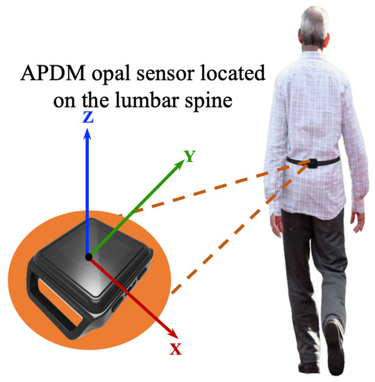
Figure 8.
Illustration of the IMU setup. APDM opal sensors were positioned on the subjects’ lower backs over the clothing using elastic straps.
3.2.1. Data Filtering
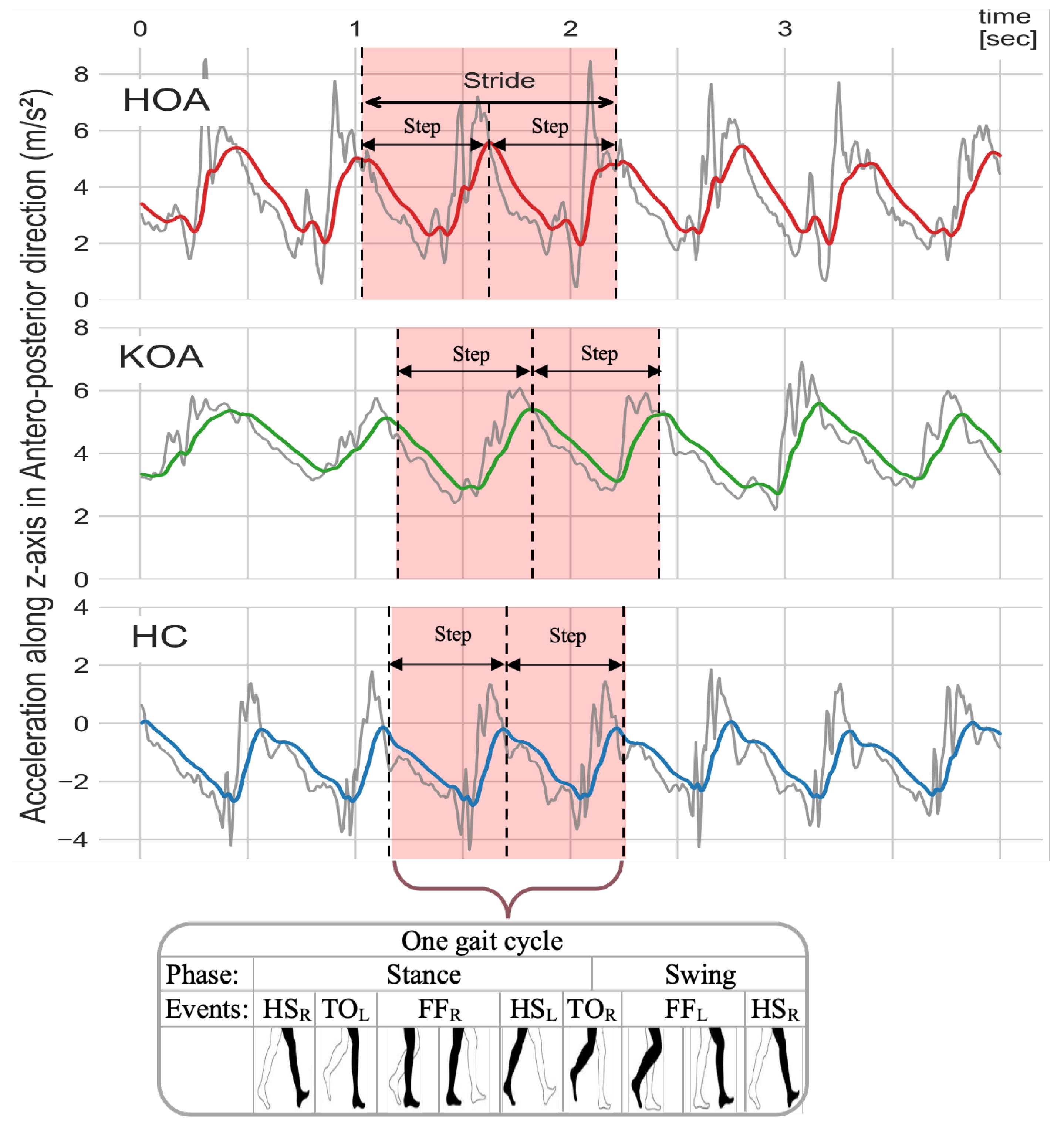
In order to generate a less spurious signal that was amenable for analyses, the AccAP signals were filtered using a fourth-order Butterworth low pass filter with a 2 Hz cut-off frequency given by Equation (1). This filtering removed noise and high-frequency components without distorting the shape of the signals. The cut-off frequency was determined by taking the average of the typical walking frequency range (between 1.6 Hz and 2.4 Hz) [91]. Figure 9 illustrates the raw and filtered AccAP signal patterns while subjects with various OA-related conditions were walking.
where is the transfer function at angular frequency , and is the cutoff frequency.
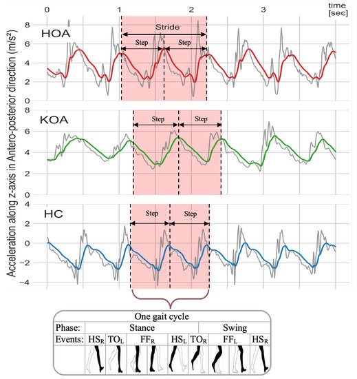
Figure 9.
Raw (gray color) and filtered AccAP (red, green, and blue) signals for HOA, KOA, and HC, respectively. The signals for HOA (red) and KOA (green) participants represent subjects who are experiencing pain, while the signal for the HC (blue) represents a subject without pain.
3.2.2. Gait Events
In order to extract STGP features, the gait cycle needs to be determined by detecting HS events in the signal for one foot. Each gait cycle includes TO events, which are used along with HS to calculate the STGP features. Identifying the HS and TO events requires signal peak detection, one of the most common GEs widely utilized in the literature [92,93], in each gait cycle to distinguish the steps. Peaks (local maxima) with very high AccAP signal amplitude occur when the heel touches the ground, and valleys (local minima) in the AccAP appear when the foot leaves the ground during walking. In this study, prior to detecting the HS and TO events, we removed the gait initiation phase (i.e., the first three steps) in order to ensure that the gait parameters were calculated from steady-state walking [94]. Then, to detect the HSs and TOs, the findpeak function from the Sensor Motion Python package was applied to the filtered AccAP signal. The findpeak method detects local maximums and/or local minimums in the given sensor signal [95]. The HS instances were tagged as local maxima peaks, while the TO instances were tagged as minimum peaks of the AccAP. Figure 10 shows an example of signals and the detected HS and TO events. To designate the right and left foot, we used the vertical axis angular velocity () signal at the instant of HS after filtering it using the fourth-order Butterworth filter with a 2 Hz cut-off. The positive deflection of indicates the heel strike of the left foot, and its negative sign implies the heel strike of the right foot [96,97].

Figure 10.
Filtered AccAP signal for HOA (purple line), KOA (orange line), and HC (blue line), and vertical angular velocity (gray line) along a few steps are depicted. Local maxima and minima in the AccAP signal correspond to HSs (filled circles) and TOs (asterisks), respectively. The red color represents the left foot, while the green color represents the right foot.
To avoid finding more than two HSs in an individual step and to eliminate the erroneous peaks from unexpected parts of the signals, we applied two thresholds: Minimal Peak Distance (MPD), the minimum distance between each peak, and Minimal Peak High (MPH). To reduce the false positive identification and the number of peaks/valleys caused by the turn phase, the MPD was set to 0.16 s. Only positive and negative peaks greater or less than MPH were considered. The MPH was determined by Equation (2):
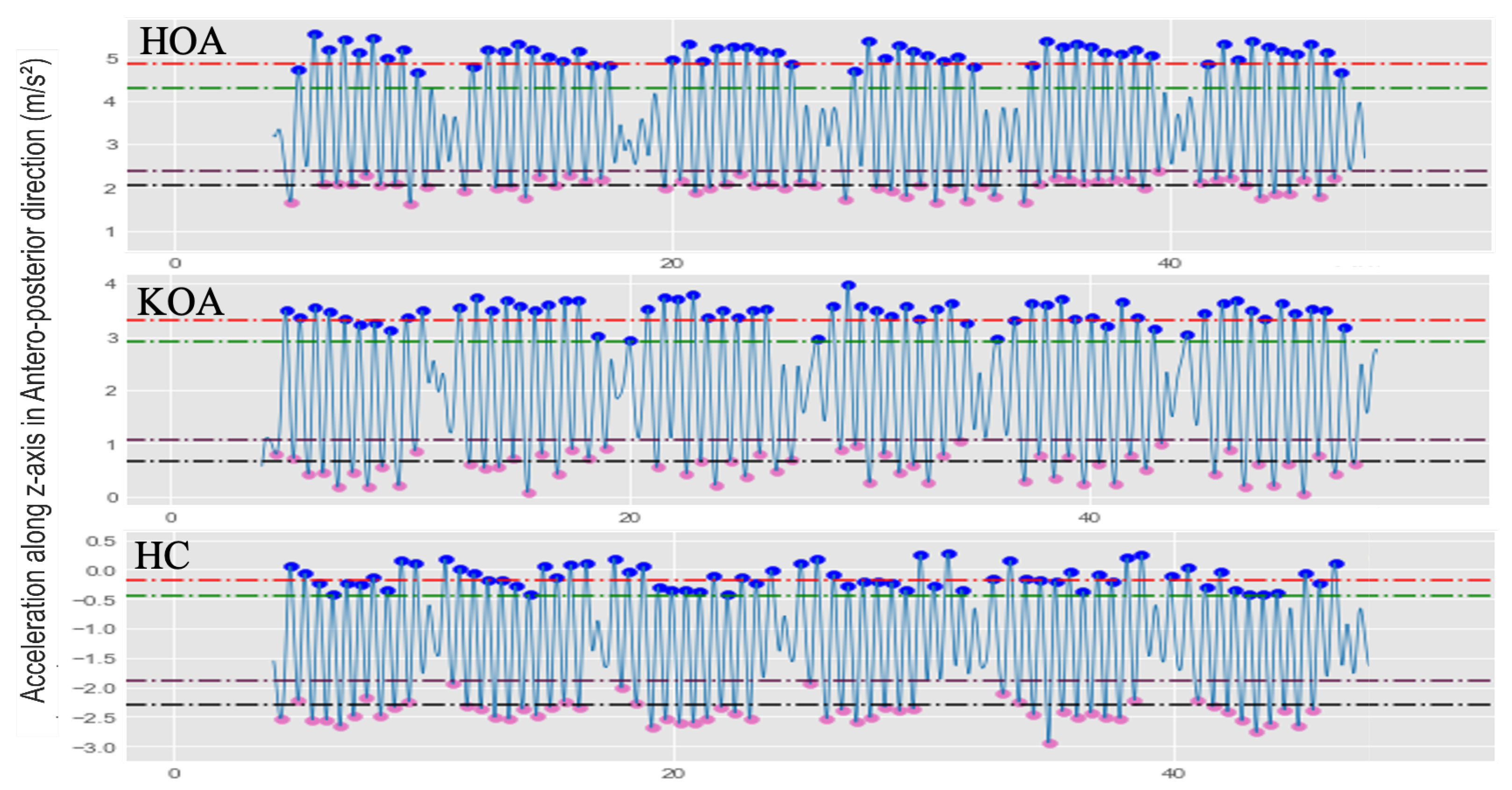
where the and are the average of peaks or valleys, and are the peaks and valleys’ standard deviation, respectively. P is the detected peak/valley at the i position (i = 0, 1, 2, …, n). The MPD and MPH threshold values were selected empirically to find the most suitable partition rate capturing only dominant peaks/valleys, which are peaks or valleys with maximum or minimum amplitude, respectively. Figure 11 shows example AccAP signals for three subjects: HOA, KOA, and HC, along with the selected MPH thresholds.
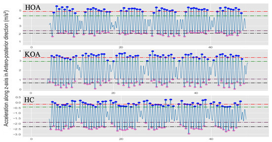
Figure 11.
Illustration examples of the various MPH thresholds to determine the local maxima and local minima for HOA, KOA, and HC subjects. The red dash line is ; the green dash line is ; the plum dash line is ; the black dash line is .
3.3. Gait Feature Extraction
After segmenting the filtered AccAP data into gait cycles, twenty-one (eleven STGPs, five Time Vars, and five Fluctuation Magnitude (FM) for temporal gait) features were computed. We define time Var as a quantifiable hallmark of gait that varies in older adults with walking impairments and FM as the amount of variation in the body’s trunk movement during walking [98,99,100]. The STGPs were averaged for each subject based on HS and TO events. We quantified time Var and FM in temporal gait parameters, including step time, stride time, swing time, stance time, and terminal double support time. We computed the coefficient of variation (%CoV) defined by Equation (3) and SD to reflect the time Var and FM, respectively, for temporal gait parameters:
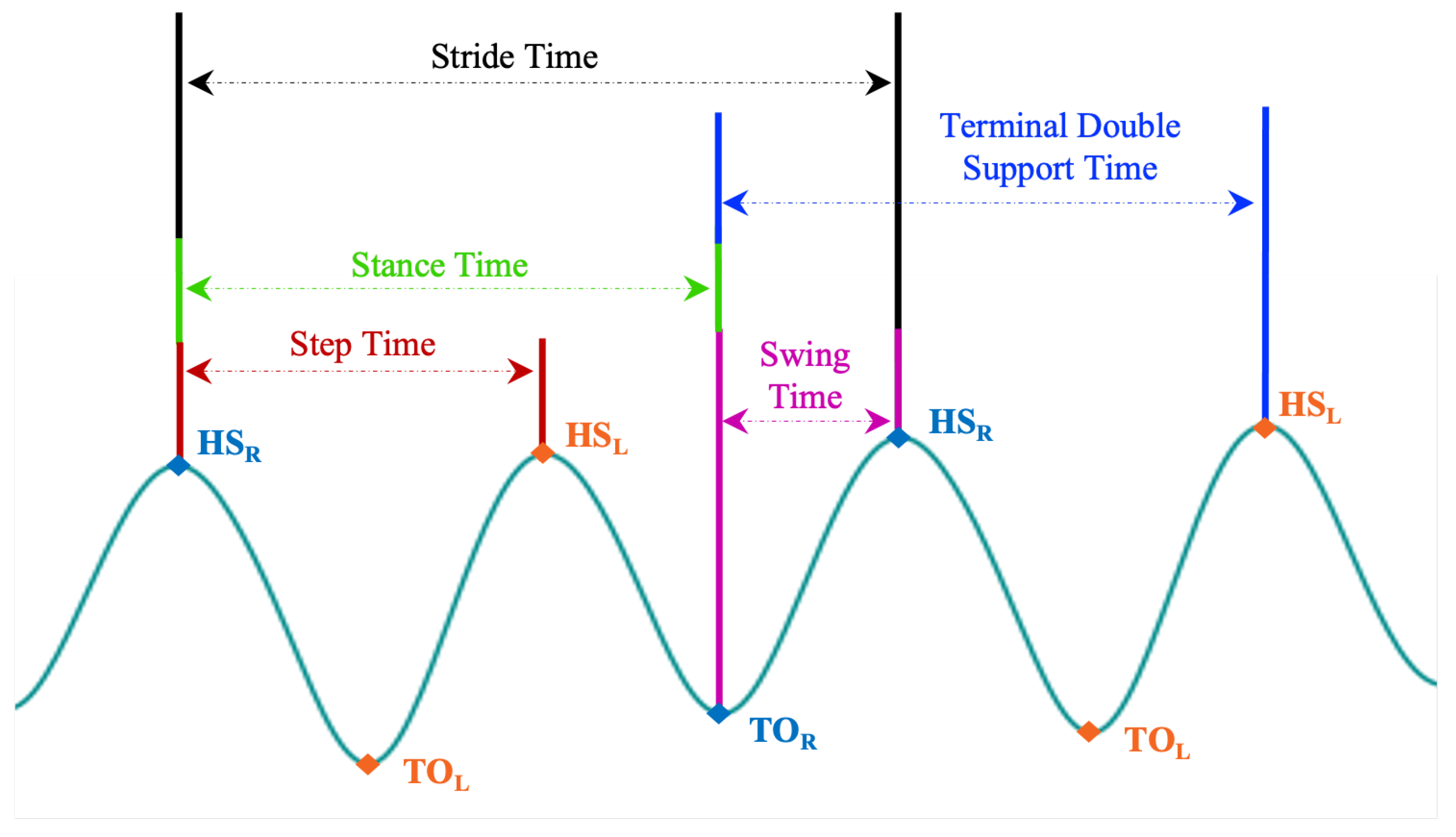
To compute the step length and stride length, we estimated the total distance (TD) for each subject in the 2 min walk by multiplying the walkway length (6 m) by the number of turns for each individual. Table 4 provides a summary of the calculated STGP descriptions using the right foot as a reference and the left foot as a contralateral foot. Figure 12 depicts how temporal gait parameters were computed on the AccAP signals.

Table 4.
Operational definitions of spatial-temporal gait parameters.

Figure 12.
Illustration of how each temporal gait feature is defined on the AccAP signal. The Heel Strike of the right foot (HS) is used as a reference. (HS) is the HS of the left foot, and TO and TO are the toe-off of the right and left foot, respectively.
3.4. Data Rescaling Procedures
Rescaling of values in a dataset is sometimes required, particularly from a machine learning and Biomechanics perspective. From a machine learning perspective, certain types of algorithms are sensitive to ranges of values, including gradient descent-based algorithms, such as LR, and distance-based algorithms, such as SVM and KNN [104]. From a biomechanics perspective, the features extracted from sensor data on human motion studies, such as accelerometer data, are influenced by participants’ physical attributes, including their age, height, body mass, and gender. Such inter-subject differences invariably increase inter-subject gait variability. Consequently, rescaling gait data based on a patient’s attributes, especially height, is frequently employed to minimize the inter-subject variation.
In this study, we utilized the following normalization procedures for each STGP, X of length n, where :
- 1.
- No normalization: use the raw spatial-temporal gait features.
- 2.
- Dataset-level normalization: shift and re-scale X using the min and max values as computed over X. This normalization results in values ranging between 0 and 1:
- 3.
- Dataset-level standardization: re-scale X to have a mean of 0 and a standard deviation of 1:
- 4.
- Subject-level normalization: subject demographics can cause variations in gait parameters causing some confounding, which ultimately reduces the ability to discern underlying pathological gait patterns. For instance, a shorter individual may naturally take a longer stride than those taken by a taller subject. When comparing two groups, these variations in gait parameters increase the influence of between-subject differences in physical characteristics and walking speed, leading to data dispersion [39]. Dimensionless (DL) equations proposed by Hof have frequently been used in prior work to normalize gait data, significantly decreasing variations in gait that are not attributable to the underlying pathological gait pattern [105]. The idea behind DL is to present the data in a non-dimensional form, representing the ratio of the feature value with subject height (h) rather than its value with a measurement unit [106,107]. Table 5 displays DL equations corresponding to measures of gait length (l), time (t), frequency (f), and velocity (v) features. In this study, we normalized each X feature by the subject’s height (h), using DL equations to improve the ML classification accuracy between the two groups.
 Table 5. Dimensionless forms related to spatial-temporal gait features.
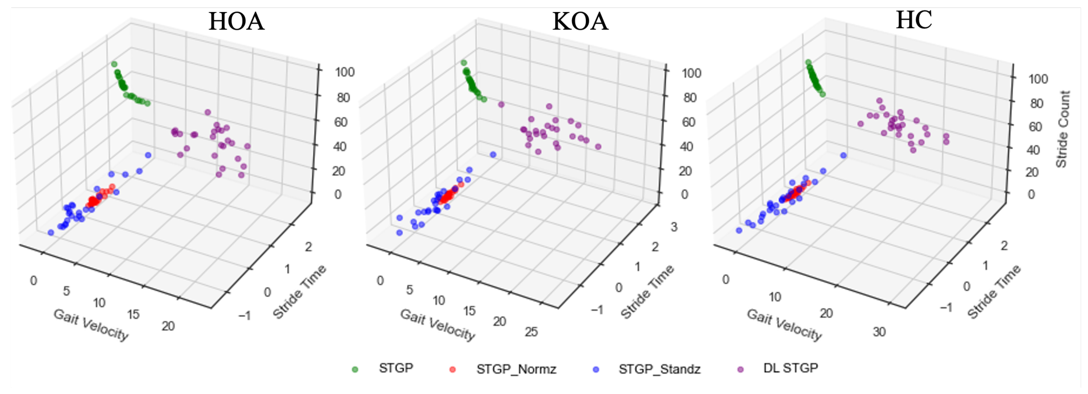
We ended up with four experimental datasets: (1) raw STGP; (2) normalized STGP (STGP-Normz); (3) standardized STGP (STGP-Standz); (4) dimensionless STGP (DL STGP). We used these datasets as input for our ML classification models. Figure 13 depicts examples of the STGP features before and after normalization for HOA, KOA, and HC data.

Figure 13.
Examples of the three STGP features (gait velocity, stride time, and stride count) before and after applying data re-scaling for HOA, KOA, and HC. The green circles represent the raw STGP (before data re-scaling). The red, blue, and purple circles represent the normalized STGP, the standardized STGP, and the dimensionless STGP, respectively.
3.5. Machine Learning Pain Classification
To distinguish between clinically moderate-to-severe pain and no-pain conditions, we investigated using various ML algorithms to classify the STGP extracted from AccAP (forward direction) signals. We then compared their performances in order to determine the best combinations of features and machine learning models. We experimented with six classifiers from various domains: linear (LR and SVM), non-linear (KNN), and tree ensemble (DT, RF, and XGB) in order to discover the optimal model for classifying HOOS/KOOS moderate-to-severe pain from no-pain. Train and test data for the classifiers were based on the STGP, STGP-Normz, STGP-Standz, and DL STGP datasets. Train and test data for the classifiers were based on the STGP, STGP-Normz, STGP-Standz, and DL STGP datasets. The best performing classifier was selected based on the best results observed.
3.6. Model Evaluation
Model performance was evaluated with the accuracy and Area Under the Curve (AUC) metrics, which are frequently used to evaluate the performance of binary classification algorithms. To avoid overfitting, a 5-fold stratified cross-validation (cv) evaluation method was utilized with results from each fold averaged (Equations (6) and (7)). We used the stratified cv to reduce experimental variance and avoid the risk of having zero positives in one or more of the folds, leading to undefined AUC.
where , the fold number in cross-validation.
3.7. Model Hyperparameter Optimization
In supervised ML, hyperparameter tuning, the task of selecting optimal hyperparameters for each ML learning algorithm is crucial for achieving the best possible results. We tuned the hyperparameters of our ML models to determine optimal hyperparameters while also avoiding overfitting by striking a balance between bias and variance. For hyperparameter tuning, the Grid search algorithm [108] was employed. In grid search, a search space is defined as a grid of given discrete hyperparameters. The grid search algorithm evaluates combinations of hyperparameter values in the grid simultaneously [109] to determine optimal values. Table 6 presents our hyperparameters optimized by grid search and their optimal values for each ML algorithm.

Table 6.
Hyperparameter tuning space for ML algorithms.
3.8. Feature Ranking
Feature ranking was applied to determine which input features were most predictive of pain levels. The RF algorithm integrates feature ranking algorithms for classification tasks, which we utilized in this work; RF has built-in feature importance computed based on the impurity or permutation importance [110]. In this work, we measured the importance scores of our features based on the impurity measure, also known as the mean decrease of impurity [111].
4. Results
The proposed OA-Pain-Sense scheme is based on STGPs extracted from AccAP data. The raw STGP and rescaling data, using normalization, standardization, and dimensionless methods, were used separately as input features to six ML algorithms (LR, SVM, KNN, DT, RF, XGB) to evaluate the performance of our proposed OA-Pain-Sense framework. The ML algorithms were applied to train and test HOA vs. HC and KOA vs. HC data with a 30%:70% split. The average accuracy and AUC values were recorded.
4.1. Data Rescaling Performance
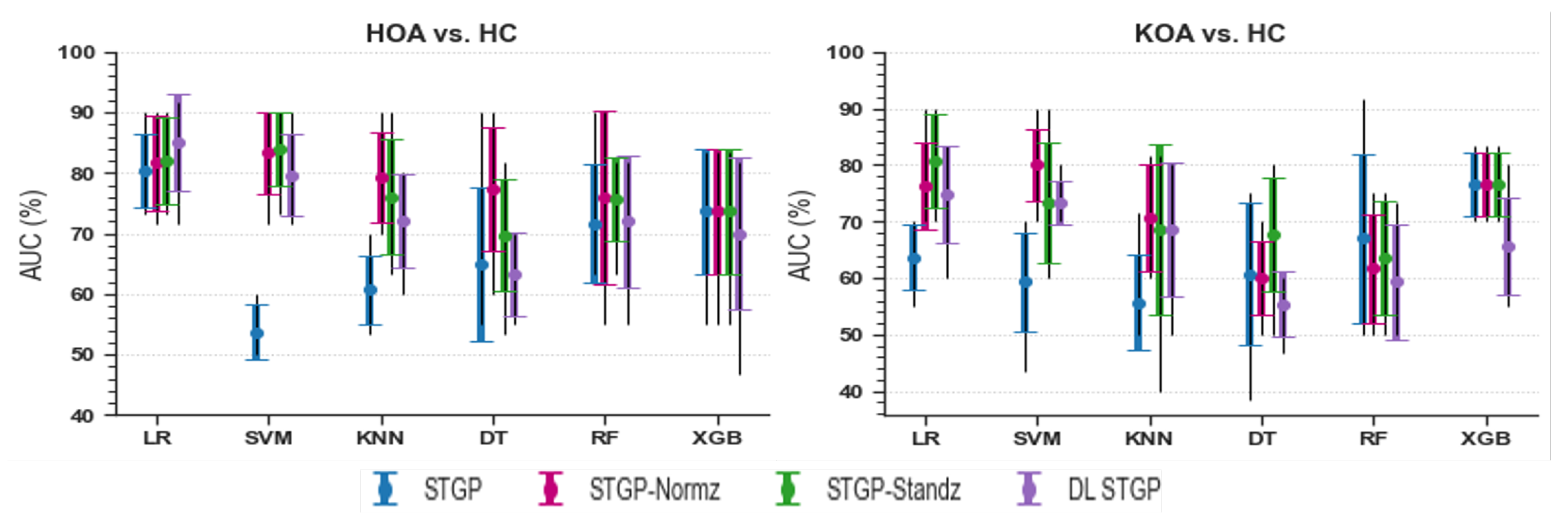
The average accuracies and AUCs of self-reported pain classifiers using the raw STGP and rescaling STGP data are depicted in Figure 14 and Figure 15. Table 7 and Table 8 present the performance of various rescaling methods. LR with raw STPG data inputs outperformed all other ML models for the classification task of HOA vs. HC (79.45% accuracy, 80.33% AUC). XGB achieved the best performance when discriminating KOA from HC (76.73% accuracy, 76.67% AUC). SVM (54.55% accuracy, 53.67% AUC) and KNN (55.45% accuracy, 55.67% AUC) with raw STGP features perform the worst for the HOA vs. HC and KOA vs. HC classification tasks, respectively, indicating that data rescaling data is necessary in order to optimize the performance of these models. Applying the rescaling methods to STGP features had no significant effect on tree ensemble methods; this could be because these methods are scale-invariant, making them insensitive to variations in data. On the other hand, it improved the performance of LR, SVM, and KNN, which are scale-variant. Different results were obtained for features with varying ranges. Overall, the accuracy and AUC results for LR using the DL STGP features for HOA vs. HC (84.91% and 85%) and the standardized STGP for KOA vs. HC (80.73% and 80.67%) were relatively high.

Figure 14.
Accuracy of baseline models using raw STGP and rescaled STGP data. The white rectangular boxes represent the best accuracy for each ML model.
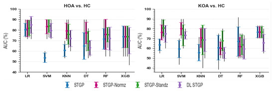
Figure 15.
Baseline models AUC using raw STGP and scaled STGP data.

Table 7.
HOA vs. HC Accuracy of ML models.

Table 8.
KOA vs. HC Accuracy of ML models.
4.2. Hyperparameter Optimization
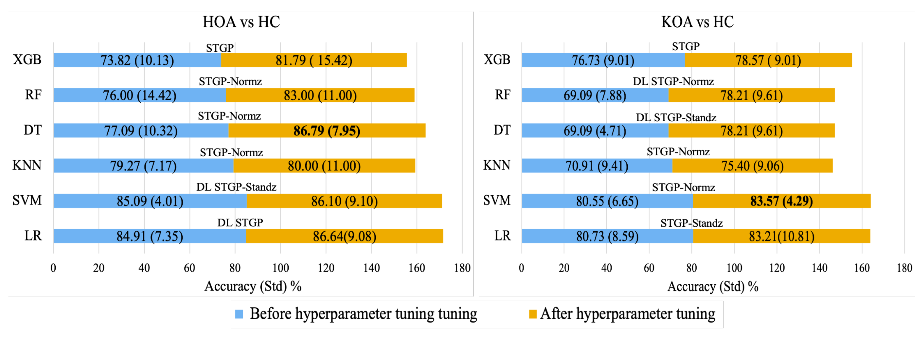
Figure 16 shows the average accuracy of ML algorithms before and after hyperparameter tuning using the grid search method. It can be observed that hyperparameter optimization improved the performance of all models. Consequently, using normalized STGP features, the best performances were achieved with the DT (86.79%) for HOA vs. HC and the SVM (83.57%) for KOA vs. HC.
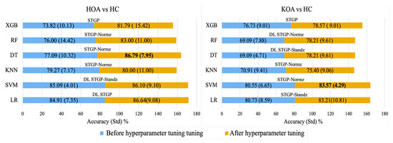
Figure 16.
Best accuracy for each baseline ML model with its input data before hyperparameter tuning (blue color) and after hyperparameter tuning (gold color).
4.3. Feature Ranking
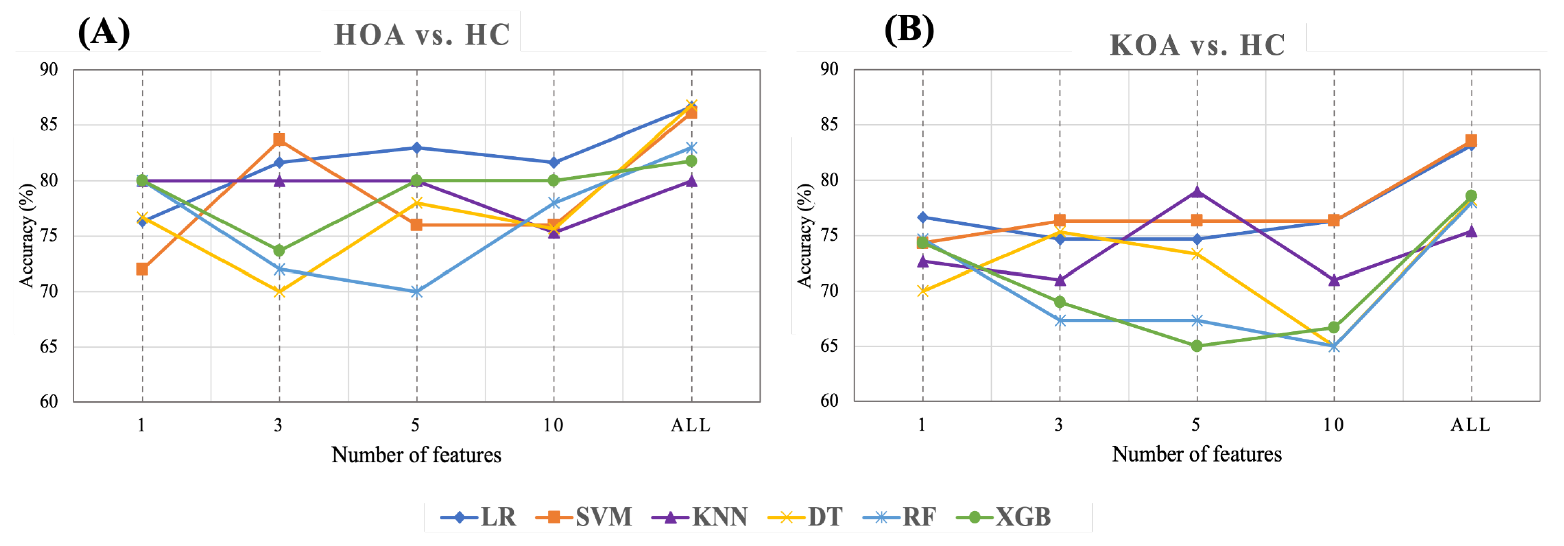
This section presents the results of feature ranking results using Random Forest, applied after hyperparameter tuning. Figure 17 exhibits the importance score of the Top 1, 3, 5, and 10 STGP features. We expected that removing less important features would improve classification performance. However, as shown in Figure 18, we achieved the best accuracy using all features for HOA vs. HC and KOA vs. HC. Regardless, noticeably, using only one feature (gait velocity), RF and XGB performed similarly to using all features and better than employing the top 3, top 5, and top 10 most important features. This is possible because of gait velocity’s high importance (predictive value).

Figure 17.
Feature ranking generated by the Random Forest. The filled circles with colors green, red, purple, and yellow indicate the 1 top, 3 top, 5 top, and 10 top features, respectively.
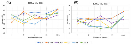
Figure 18.
Accuracy of ML with top 1, 3, 5, 10, all STGP features for (A) HOA vs. HC and (B) KOA vs. HC.
As shown in Table 9 and Figure 18A, for HOA vs. HC, the top three features (gait velocity, stride time, stride count) represented 83.67% of the accuracy when using SVM, which was close to the performance achieved using all features. LR outperforms all other classifiers with an accuracy of 83% when utilizing the five top features (gait velocity, stride time, stride count, step count, step time). Using the 10 top features (gait velocity, stride time, stride count, step count, step time, cadence, stride length, TdsT SD, step length, stride time SD) reduces the accuracy of all ML models except RF and XGB when compared to using the top three and top five features. It is noteworthy that KNN achieved the same accuracy (80%) using the top 1, top 3, top 5, and all features.

Table 9.
HOA vs. HC accuracy of feature ranking.
Table 10 and Figure 18B show the results of feature ranking for predicting KOA vs. HC. With only the gait velocity feature, LR has the highest accuracy (76.67%). Similar accuracy was achieved using the 3 top features (gait velocity, cadence, stride time) and 10 top features (gait velocity, cadence, stride time, stride length, step length, step time, step count, stride count, swing time Var, Terminal Double Support Time Var). Of all ML models, KNN achieved the best accuracy (79%) when using the five top features (Gait Velocity, Cadence, Stride time, Stride length, and Step length). RF and XGB had a lower accuracy when using the top 3, top 5, and top 10 features.

Table 10.
KOA vs. HC accuracy of feature ranking.
5. Discussion
Using un-normalized STGPs as ML features to predict self-reported HOOS/KOOS moderate–severe pain levels of older patients with end-stage HKOA achieved encouraging results. Specifically, the results of LR and XGB using HOA vs. HC (shown in Table 9) and KOA vs. HC data (shown in Table 10), respectively, support our hypothesis that ML can achieve reasonable classification performance of whether an HKOA patient has pain or not. These results provide a strong basis for our OA-Pain-Sense framework, which could, in turn, lead to improvements in clinical pain management.
Rescaling STGP Features using dataset-level methods improved the performance of ML models: Referring to the results in Table 7 and Table 8 and depicted in Figure 14 and Figure 15, the dataset-level rescaling methods significantly improved the SVM and KNN performance and did reduce the performance of XGB. These results align with the literature that distance-based ML algorithms are sensitive to dominant features, degrading the algorithm’s performance. Further, they reflect the fact that XGB is invariant to feature rescaling [112]. On the other hand, the LR results disagree with the findings of Adeyemo et al.’s study [113], in which LR performs inadequately in rescaled data. The mean accuracy of the LR with rescaled STGP features increased by ∼2% and ∼13–17% for HOA and KOA, respectively. The DT and RF performance improved after rescaling based on the HOA vs. HC classification results. However, the RF results were unsatisfactory after employing the rescaled STGP for KOA vs. HC classification, whereas the DT had minimal improvement. Overall, the improvements achieved by data rescaling methods are data-dependent, which is in line with the findings of prior work [113,114].
Dimensionless normalization of features was able to correct the effects of physiological variation on ML performance: Specifically, reducing data dispersion caused by physiological variations using DL equations resulted in noticeable improvements in the LR, SVM, and KNN accuracies in the ranges of ∼6–24% and ∼11–13% for HOA vs. HC and KOA vs. HC, respectively. These results were significantly higher than using the results achieved using raw STGP features as observed in Table 7 and Table 8. Nevertheless, dimensionless normalization caused the performance of the tree ensemble models to drop marginally compared to their performance using raw STGP features; we speculate that this may be due to the small size of the dataset and the participants’ demography.
The effects of the data rescaling methods on various ML classification algorithms were dataset-dependent: Comparing the DL equations to the dataset-level normalization and standardization algorithms, it can be observed that most ML models achieved the best average accuracy and AUC when classifying STGPs rescaled using the min-max normalization or z-score algorithms. Using the HOA vs. HC data, achieved the best average accuracy (84.91%) of the LR model when classifying DL STGPs. It also had the highest classification performance with an average accuracy of 80.73% when using STGP-Stanz extracted from KOA and HC data. The LR results indicate that the STGP features reasonably correlate with HOOS/KOOS pain levels. In conclusion, utilizing the dataset rescaling methods seems to perform better than other normalization and rescaling methods explored on some of our selected ML algorithms. However, the specific ML methods on which dataset rescaling improved performance depended on the data structure. Thus, while there is no one-fits-all solution, some dataset rescaling methods can be recommended.
Applying a hyperparameter tuning technique to the best models increased their accuracies slightly: Hyperparameter tuning achieved the highest performance depending on the input features (raw STGPs or rescaled STPGs) with classification performance improvements in the range of ∼2–10%. We believe such a technique requires a large dataset in order to observe noticeable differences due to hyperparameter tuning. Alternate techniques should be considered to achieve optimal models on a small dataset. Regardless, the results in Figure 16 present promising preliminary evidence for the OA-Pain-Sense framework, which could be generalizable to using STGP data extracted from an accelerometer in any wearable sensor, including smartphone position on the human body trunk regions.
Reducing the number of features also reduced the performance (accuracies) of most of the ML models: As shown in Figure 18, we explored the effects of reducing the number of features on ML performance in order to discover the optimal number of features after hyperparameter optimization (Figure 17). Removing features did not improve the performance of the ML models. We believe that this may be because of the relatively small sample size. Regardless of changes in the ML models’ performance, the following was noticed after reducing the number of features:
- Gait velocity (GV) was the most important feature in predicting HOOS/KOOS pain levels. With only this feature, the KNN, RF, and XGB achieved 80%, and LR gained 76.67% for HOA vs. HC and KOA vs. HC, respectively. Previous studies reported that individuals with HKOA walk slower than healthy controls of the same age. Thus, our results for the top 1 feature agree with the results of prior research [53,115].
- Employing the top 3 STPG features extracted from HOA and HC data achieved a mean accuracy (83.67% with SVM) closer by ∼3% to using all 21 STGP features (86.79% with DT).
- KNN performance improved by ∼4%, with the top five features outperforming using all STPGs for KOA and HC data.
These findings, after applying the feature ranking technique, presented new insights and suggest a way to investigate more compelling features for classifying HOOS/KOOS pain levels.
Comparison with other studies is challenging because different sets of features were used and not only STGP features: There is a lack of research on this area, especially in the HOA population. Most prior studies were conducted to predict pain in KOA, while there is only one study on HOA. Table 11 compares our proposed OA-Pain-Sense comprehensively with all previous studies that predict pain in the HOA or KOA population using ML algorithms. We intended to compare our work using STGPs extracted from only one axis signal with those using other kinds of features. Table 11 indicates that our method performs better than state-of-the-art methods for KOA and HC. The highest accuracy was obtained using our method, outperforming all previous and related studies except that of Alexos et al. [70]. However, we believe our work has advantages over Alexos et al. work. We predicted the self-reported pain for both legs while Alexos et al. predicted each leg’s pain. We achieved an accuracy (83.57%) between those achieved by Alexos et al. accuracies (82.50% and 84.30%). We used the STGP features, which are more reliable, robust, and clinically validated. Moreover, our prediction approach using STGPs is more practical in the real world than using the baseline questionnaire data used by Alexos et al.

Table 11.
Comparison of performance achieved by prior related work.
Study limitations: A few limitations should be acknowledged and considered in our future work. Our study population was exclusively elderly subjects with unilateral end-stage hip/knee OA, which raises a question on the generalizability of our outcomes to other populations. The datasets we classified were small, and subjects were not gender-matched (42 males and 36 females), which may have influenced our ML model results. Finally, the reliance on patient self-reports of their pain introduces bias, and the lack of a gold standard or reference data limited our ability to evaluate the performance of the peak detection algorithm used to identify gait events in our preprocessing step.
Future work: We plan to collect more data from patients at different stages of HKOA and ages and apply the proposed framework to determine the effectiveness of our OA-Pain-Sense framework in even more realistic scenarios. Furthermore, we plan to combine features from various physical activities such as sit-to-stand, stand-to-sit, and stair ascent and descent with gait features into our model to improve the robustness of our model as these features enhance our model and reduce confounding. We also plan to explore emerging deep learning models as more data becomes available, which may increase the robustness and reliability of the OA-Pain-Sense framework. Moreover, we plan to perform a comprehensive analysis of HKOA gait abnormalities and compare our findings to normative STGP values from the medical perspective of HKOA patients. Finally, we would like to validate OA-Pain-Sense in a live deployment.
6. Conclusions
This paper investigated the feasibility of OA-Pain-sense, a machine learning framework to classify the HOOS/KOOS self-report pain level in HKOA patients. Data were collected from IMU APDM Opal attached to each subject’s lumbar while performing a 2 min walk at a self-selected pace. Spatial-Temporal Gait Parameters (STGPs) were extracted from only anterior-posterior accelerometer data and then rescaled using dataset-level and subject-level rescaling methods. Various machine learning algorithms were utilized to classify the STGPs in order to predict the pain of HKOA patients with further improvements resulting from hyperparameter tuning using grid search. Feature ranking using Random Forest was conducted in this study to demonstrate the impact of reducing feature numbers on the models’ performance. The proposed method achieved an average classification accuracy of 86.79% with DT and 83.57% with SVM for hip OA vs. healthy control and knee OA vs. healthy control, respectively. The results of this work demonstrate that STGPs can serve as reliable biomarkers and predictive ML features for predicting whether HKOA patients have moderate–severe pain or not. We envision the possible deployment of the eventual system on smartphones and in natural settings.
Author Contributions
Conceptualization, W.S.A., E.A., J.K., and P.F.; methodology, W.S.A. and E.A.; software, W.S.A.; validation, W.S.A., and E.A.; formal analysis, W.S.A. and E.A.; investigation, W.S.A. and E.A.; resources, data curation, W.S.A.; writing—original draft preparation, W.S.A. and E.A.; writing—review and editing, W.S.A. and E.A.; visualization, W.S.A.; supervision, E.A.; project administration, W.S.A. and E.A. All authors have read and agreed to the published version of the manuscript.
Funding
This research received no external funding.
Institutional Review Board Statement
Not applicable.
Informed Consent Statement
Not applicable.
Data Availability Statement
Not applicable.
Acknowledgments
Conflicts of Interest
The authors declare no conflict of interest.
Abbreviations
The following abbreviations are used in this manuscript:
| OA | Osteoarthritis |
| HKOA | Hip and Knee Osteoarthritis |
| HOA | Hip Osteoarthritis |
| KOA | Knee Osteoarthritis |
| HOOS | Osteoarthritis Outcome Score |
| KOOS | Knee Injury and Osteoarthritis Outcome Score |
| WOMAC | Western Ontario and McMaster Universities Osteoarthritis Index |
| IMU | Inertial Measurement Unit |
| STGP | Spatiotemporal Gait Parameters |
| ML | Machine learning |
| AP | Anterior-Posterior |
| AccAP | P Acceleration |
| Var | Variability |
| FM | Fluctuation Magnitude |
| DL | Dimensionless |
| SD | Standard Deviation |
References
- Wang, A.; Lo, A.; Ubhi, K.; Cameron, T. Small and Transient Effect of Cannabis Oil for Osteoarthritis-Related Joint Pain: A Case Report. Can. J. Hosp. Pharm. 2021, 74, 156–158. [Google Scholar] [CrossRef]
- Favre, J.; Jolles, B.M. Gait analysis of patients with knee osteoarthritis highlights a pathological mechanical pathway and provides a basis for therapeutic interventions. EFORT Open Rev. 2016, 1, 368–374. [Google Scholar] [CrossRef] [PubMed]
- Dong, Y.; Zhang, B.; Yang, Q.; Zhu, J.; Sun, X. The effects of platelet-rich plasma injection in knee and hip osteoarthritis: A meta-analysis of randomized controlled trials. Clin. Rheumatol. 2021, 40, 263–277. [Google Scholar] [CrossRef] [PubMed]
- Liu, K.; Chen, Y.; Miao, Y.; Xue, F.; Yin, J.; Wang, L.; Li, G. Microstructural and histomorphological features of osteophytes in late-stage human knee osteoarthritis with varus deformity. Jt. Bone Spine 2022, 89, 105353. [Google Scholar] [CrossRef] [PubMed]
- Hunter, D.J.; March, L.; Chew, M. Osteoarthritis in 2020 and beyond: A Lancet Commission. Lancet 2020, 396, 1711–1712. [Google Scholar] [CrossRef]
- Callahan, L.F.; Cleveland, R.J.; Allen, K.D.; Golightly, Y. Racial/Ethnic, Socioeconomic, and Geographic Disparities in the Epidemiology of Knee and Hip Osteoarthritis. Rheum. Dis. Clin. 2021, 47, 1–20. [Google Scholar] [CrossRef]
- Dell’Isola, A.; Pihl, K.; Turkiewicz, A.; Hughes, V.; Zhang, W.; Bierma-Zeinstra, S.; Prieto-Alhambra, D.; Englund, M. Risk of comorbidities following physician-diagnosed knee or hip osteoarthritis: A register-based cohort study. Arthritis Care Res. 2021, 74, 1689–1695. [Google Scholar] [CrossRef]
- Ferreira, G.E.; McLachlan, A.J.; Lin, C.W.C.; Zadro, J.R.; Abdel-Shaheed, C.; O’Keeffe, M.; Maher, C.G. Efficacy and safety of antidepressants for the treatment of back pain and osteoarthritis: Systematic review and meta-analysis. BMJ 2021, 372, m4825. [Google Scholar] [CrossRef]
- Cui, A.; Li, H.; Wang, D.; Zhong, J.; Chen, Y.; Lu, H. Global, regional prevalence, incidence and risk factors of knee osteoarthritis in population-based studies. EClinicalMedicine 2020, 29, 100587. [Google Scholar] [CrossRef]
- van Berkel, A.C.; Schiphof, D.; Waarsing, J.H.; Runhaar, J.; van Ochten, J.M.; Bindels, P.J.; Bierma-Zeinstra, S.M. 10-Year natural course of early hip osteoarthritis in middle-aged persons with hip pain: A CHECK study. Ann. Rheum. Dis. 2021, 80, 487–493. [Google Scholar] [CrossRef]
- OA Prevalence & Burden Osteoarthritis Prevention and Management in Primary Care. Available online: https://oaaction.unc.edu/oa-module/oa-prevalence-and-burden/ (accessed on 3 October 2022).
- Zolio, L.; Lim, K.Y.; McKenzie, J.E.; Yan, M.K.; Estee, M.; Hussain, S.M.; Cicuttini, F.; Wluka, A. Systematic review and meta-analysis of the prevalence of neuropathic-like pain and/or pain sensitisation in people with knee and hip osteoarthritis. Osteoarthr. Cartil. 2021, 29, 1096–1116. [Google Scholar] [CrossRef] [PubMed]
- Hawker, G.A. The challenge of pain for patients with OA. HSSJ 2012, 8, 42–44. [Google Scholar] [CrossRef] [PubMed]
- Verma, D.K.; Kumari, P.; Kanagaraj, S. Engineering Aspects of Incidence, Prevalence, and Management of Osteoarthritis: A Review. Ann. Biomed. Eng. 2022, 50, 237–252. [Google Scholar] [CrossRef] [PubMed]
- Lai, Y.F.; Lin, P.C.; Chen, C.H.; Chen, J.L.; Hsu, H.T. Current status and changes in pain and activities of daily living in elderly patients with osteoarthritis before and after unilateral total knee replacement surgery. J. Clin. Med. 2019, 8, 221. [Google Scholar] [CrossRef]
- Wu, J.; Qian, Z.; Xu, R.; Liu, J.; Ren, L.; Ren, L. Association Between Pain in Knee Osteoarthritis and Mechanical Properties of Soft Tissue Around Knee Joint. IEEE Access 2021, 9, 14599–14607. [Google Scholar] [CrossRef]
- Nilsdotter, A.K.; Lohmander, L.S.; Klässbo, M.; Roos, E.M. Hip disability and osteoarthritis outcome score (HOOS)–validity and responsiveness in total hip replacement. BMC Musculoskelet. Disord. 2003, 4, 10. [Google Scholar] [CrossRef]
- Roos, E.M.; Lohmander, L.S. The Knee injury and Osteoarthritis Outcome Score (KOOS): From joint injury to osteoarthritis. Health Qual. Life Outcomes 2003, 1, 64. [Google Scholar] [CrossRef] [PubMed]
- Jared R H Foran, MD, F. DISEASES & CONDITIONS Osteoarthritis of the Hip. Available online: https://orthoinfo.aaos.org/en/diseases–conditions/osteoarthritis-of-the-hip (accessed on 26 March 2022).
- Katz, J.N.; Arant, K.R.; Thornhill, T.S. Knee Osteoarthritis. In Principles of Orthopedic Practice for Primary Care Providers; Springer: Berlin/Heidelberg, Germany, 2021; pp. 413–423. [Google Scholar]
- Liu, D.; Cheng, D.; Houle, T.T.; Chen, L.; Zhang, W.; Deng, H. Machine learning methods for automatic pain assessment using facial expression information: Protocol for a systematic review and meta-analysis. Medicine 2018, 97, e13421. [Google Scholar] [CrossRef]
- Herr, K.A.; Garand, L. Assessment and measurement of pain in older adults. Clin. Geriatr. Med. 2001, 17, 457–478. [Google Scholar] [CrossRef]
- Purser, J.L.; Golightly, Y.M.; Feng, Q.; Helmick, C.G.; Renner, J.B.; Jordan, J.M. Association of slower walking speed with incident knee osteoarthritis–related outcomes. Arthritis Care Res. 2012, 64, 1028–1035. [Google Scholar]
- Vincent, K.R.; Conrad, B.P.; Fregly, B.J.; Vincent, H.K. The pathophysiology of osteoarthritis: A mechanical perspective on the knee joint. PM R 2012, 4, S3–S9. [Google Scholar] [CrossRef] [PubMed]
- Clermont, C.A.; Barden, J.M. Accelerometer-based determination of gait variability in older adults with knee osteoarthritis. Gait Posture 2016, 50, 126–130. [Google Scholar] [CrossRef] [PubMed]
- Bolink, S.; Van Laarhoven, S.; Lipperts, M.; Heyligers, I.; Grimm, B. Inertial sensor motion analysis of gait, sit–stand transfers and step-up transfers: Differentiating knee patients from healthy controls. Physiol. Meas. 2012, 33, 1947. [Google Scholar] [CrossRef] [PubMed]
- Suri, A.; Rosso, A.L.; VanSwearingen, J.; Coffman, L.M.; Redfern, M.S.; Brach, J.S.; Sejdić, E. Mobility of older adults: Gait quality measures are associated with life-space assessment scores. J. Gerontol. Ser. A 2021, 76, e299–e306. [Google Scholar] [CrossRef] [PubMed]
- Godfrey, A.; Del Din, S.; Barry, G.; Mathers, J.; Rochester, L. Instrumenting gait with an accelerometer: A system and algorithm examination. Med. Eng. Phys. 2015, 37, 400–407. [Google Scholar] [CrossRef]
- Roberts, M.; Mongeon, D.; Prince, F. Biomechanical parameters for gait analysis: A systematic review of healthy human gait. Phys. Ther. Rehabil 2017, 4, 6. [Google Scholar] [CrossRef]
- Baraz, M.; Farahpour, N.; Karimi, M.T.; Rezaee, M.R. Assessment of Spatiotemporal Gait Parameters in Patients with non-specific Chronic Low Back Pain with and without pronated feet. J. Res. Sport Rehabil. 2020, 8, 1–9. [Google Scholar]
- Lopresti, A.L.; Smith, S.J.; Jackson-Michel, S.; Fairchild, T. An Investigation into the Effects of a Curcumin Extract (Curcugen®) on Osteoarthritis Pain of the Knee: A Randomised, Double-Blind, Placebo-Controlled Study. Nutrients 2022, 14, 41. [Google Scholar] [CrossRef]
- Pop, P.A.; Ungur, P.; Lazar, L.; Corbu, S.; Marcu, F.M. Treatment solutions of synovial joints and recovery processes of patients with hip and knee osteoarthritis. In Proceedings of the ASME International Mechanical Engineering Congress and Exposition, Lake Buena Vista, FL, USA, 13–19 November 2009; Volume 43758, pp. 49–58. [Google Scholar]
- Zeni, J., Jr.; Pozzi, F.; Abujaber, S.; Miller, L. Relationship between physical impairments and movement patterns during gait in patients with end-stage hip osteoarthritis. J. Orthop. Res. 2015, 33, 382–389. [Google Scholar] [CrossRef]
- Ornetti, P.; Maillefert, J.F.; Laroche, D.; Morisset, C.; Dougados, M.; Gossec, L. Gait analysis as a quantifiable outcome measure in hip or knee osteoarthritis: A systematic review. Jt. Bone Spine 2010, 77, 421–425. [Google Scholar] [CrossRef]
- Ardestani, M.M.; Wimmer, M.A. Can a linear combination of gait principal component vectors identify hip OA stages? J. Biomech. 2016, 49, 2023–2030. [Google Scholar] [CrossRef]
- Tunca, C.; Salur, G.; Ersoy, C. Deep learning for fall risk assessment with inertial sensors: Utilizing domain knowledge in spatio-temporal gait parameters. IEEE J. Biomed. Health Inform. 2019, 24, 1994–2005. [Google Scholar] [CrossRef]
- Khera, P.; Kumar, N. Novel machine learning-based hybrid strategy for severity assessment of Parkinson’s disorders. Med. Biol. Eng. Comput. 2022, 60, 811–828. [Google Scholar] [CrossRef] [PubMed]
- Das, R.; Khera, P.; Saxena, S.; Kumar, N. Automated Gait Classification Using Spatio-Temporal and Statistical Gait Features. In Soft Computing: Theories and Applications; Springer: Berlin/Heidelberg, Germany, 2022; pp. 491–500. [Google Scholar]
- Wahid, F.; Begg, R.K.; Hass, C.J.; Halgamuge, S.; Ackland, D.C. Classification of Parkinson’s disease gait using spatial-temporal gait features. IEEE J. Biomed. Health Inform. 2015, 19, 1794–1802. [Google Scholar] [CrossRef] [PubMed]
- Briggs, R.; Carey, D.; Claffey, P.; McNicholas, T.; Donoghue, O.; Kennelly, S.P.; Kenny, R.A. Do differences in spatiotemporal gait parameters predict the risk of developing depression in later life? J. Am. Geriatr. Soc. 2019, 67, 1050–1056. [Google Scholar] [CrossRef] [PubMed]
- Barth, A.T.; Boudaoud, B.; Brantley, J.S.; Chen, S.; Cunningham, C.L.; Kim, T.; Powell, H.C., Jr.; Ridenour, S.A.; Lach, J.; Bennett, B.C. Longitudinal high-fidelity gait analysis with wireless inertial body sensors. In Proceedings of the Wireless Health 2010, San Diego, CA, USA, 5–7 October 2010; pp. 192–193. [Google Scholar]
- Kressig, R.W.; Beauchet, O. Guidelines for clinical applications of spatio-temporal gait analysis in older adults. Aging Clin. Exp. Res. 2006, 18, 174–176. [Google Scholar] [CrossRef]
- Chen, D.; Cai, Y.; Qian, X.; Ansari, R.; Xu, W.; Chu, K.C.; Huang, M.C. Bring gait lab to everyday life: Gait analysis in terms of activities of daily living. IEEE Internet Things J. 2019, 7, 1298–1312. [Google Scholar] [CrossRef]
- Fernández-Gorgojo, M.; Salas-Gómez, D.; Sánchez-Juan, P.; Barbado, D.; Laguna-Bercero, E.; Pérez-Núñez, M. Clinical Assessment, Gait Analysis and Reliability of Measurement with the G Walk Inertial Sensor in Subjects with Ankle Fracture 6 Months After Surgery; Research Square: Durham, NC, USA, 2022. [Google Scholar]
- Chen, S.; Lach, J.; Lo, B.; Yang, G.Z. Toward pervasive gait analysis with wearable sensors: A systematic review. IEEE J. Biomed. Health Inform. 2016, 20, 1521–1537. [Google Scholar] [CrossRef]
- Wang, S.; Cai, Y.; Hase, K.; Uchida, K.; Kondo, D.; Saitou, T.; Ota, S. Estimation of knee joint angle during gait cycle using inertial measurement unit sensors: A method of sensor-to-clinical bone calibration on the lower limb skeletal model. J. Biomech. Sci. Eng. 2022, 17, 21-00196. [Google Scholar] [CrossRef]
- Kobsar, D.; Charlton, J.M.; Tse, C.T.; Esculier, J.F.; Graffos, A.; Krowchuk, N.M.; Thatcher, D.; Hunt, M.A. Validity and reliability of wearable inertial sensors in healthy adult walking: A systematic review and meta-analysis. J. Neuroeng. Rehabil. 2020, 17, 62. [Google Scholar] [CrossRef]
- Anwary, A.R.; Yu, H.; Vassallo, M. Optimal foot location for placing wearable IMU sensors and automatic feature extraction for gait analysis. IEEE Sens. J. 2018, 18, 2555–2567. [Google Scholar] [CrossRef]
- Seel, T.; Raisch, J.; Schauer, T. IMU-based joint angle measurement for gait analysis. Sensors 2014, 14, 6891–6909. [Google Scholar] [CrossRef] [PubMed]
- Ferreira, R.N.; Ribeiro, N.F.; Santos, C.P. Fall Risk Assessment Using Wearable Sensors: A Narrative Review. Sensors 2022, 22, 984. [Google Scholar] [CrossRef] [PubMed]
- Liikavainio, T.; Bragge, T.; Hakkarainen, M.; Karjalainen, P.A.; Arokoski, J.P. Gait and muscle activation changes in men with knee osteoarthritis. Knee 2010, 17, 69–76. [Google Scholar] [CrossRef]
- Bolink, S.A.; Brunton, L.R.; van Laarhoven, S.; Lipperts, M.; Heyligers, I.C.; Blom, A.W.; Grimm, B. Frontal plane pelvic motion during gait captures hip osteoarthritis related disability. Hip Int. 2015, 25, 413–419. [Google Scholar] [CrossRef]
- Ismailidis, P.; Kaufmann, M.; Clauss, M.; Pagenstert, G.; Eckardt, A.; Ilchmann, T.; Mündermann, A.; Nüesch, C. Kinematic changes in severe hip osteoarthritis measured at matched gait speeds. J. Orthop. Res. 2021, 39, 1253–1261. [Google Scholar] [CrossRef]
- Chen, W.; Xu, Y.; Wang, J.; Zhang, J. Kinematic analysis of human gait based on wearable sensor system for gait rehabilitation. J. Med. Biol. Eng. 2016, 36, 843–856. [Google Scholar] [CrossRef]
- Grip, H.; Nilsson, K.G.; Häger, C.K.; Lundström, R.; Öhberg, F. Does the femoral head size in hip arthroplasty influence lower body movements during squats, gait and stair walking? A clinical pilot study based on wearable motion sensors. Sensors 2019, 19, 3240. [Google Scholar] [CrossRef]
- Barrois, R.; Gregory, T.; Oudre, L.; Moreau, T.; Truong, C.; Aram Pulini, A.; Vienne, A.; Labourdette, C.; Vayatis, N.; Buffat, S.; et al. An automated recording method in clinical consultation to rate the limp in lower limb osteoarthritis. PLoS ONE 2016, 11, e0164975. [Google Scholar] [CrossRef]
- Calliess, T.; Bocklage, R.; Karkosch, R.; Marschollek, M.; Windhagen, H.; Schulze, M. Clinical evaluation of a mobile sensor-based gait analysis method for outcome measurement after knee arthroplasty. Sensors 2014, 14, 15953–15964. [Google Scholar] [CrossRef]
- Christiansen, C.L.; Bade, M.J.; Paxton, R.J.; Stevens-Lapsley, J.E. Measuring movement symmetry using tibial-mounted accelerometers for people recovering from total knee arthroplasty. Clin. Biomech. 2015, 30, 732–737. [Google Scholar] [CrossRef] [PubMed]
- Mobbs, R.J.; Perring, J.; Raj, S.M.; Maharaj, M.; Yoong, N.K.M.; Sy, L.W.; Fonseka, R.D.; Natarajan, P.; Choy, W.J. Gait metrics analysis utilizing single-point inertial measurement units: A systematic review. Mhealth 2022, 8, 9. [Google Scholar] [CrossRef] [PubMed]
- Jarchi, D.; Pope, J.; Lee, T.K.; Tamjidi, L.; Mirzaei, A.; Sanei, S. A review on accelerometry-based gait analysis and emerging clinical applications. IEEE Rev. Biomed. Eng. 2018, 11, 177–194. [Google Scholar] [CrossRef] [PubMed]
- Barden, J.M.; Clermont, C.A.; Kobsar, D.; Beauchet, O. Accelerometer-based step regularity is lower in older adults with bilateral knee osteoarthritis. Front. Hum. Neurosci. 2016, 10, 625. [Google Scholar] [CrossRef] [PubMed]
- Thang, H.M.; Viet, V.Q.; Thuc, N.D.; Choi, D. Gait identification using accelerometer on mobile phone. In Proceedings of the 2012 International Conference on Control, Automation and Information Sciences (ICCAIS), Saigon, Vietnam, 26–29 November 2012; pp. 344–348. [Google Scholar]
- Bugané, F.; Benedetti, M.; Casadio, G.; Attala, S.; Biagi, F.; Manca, M.; Leardini, A. Estimation of spatial-temporal gait parameters in level walking based on a single accelerometer: Validation on normal subjects by standard gait analysis. Comput. Methods Programs Biomed. 2012, 108, 129–137. [Google Scholar] [CrossRef]
- Hickey, A.; Gunn, E.; Alcock, L.; Del Din, S.; Godfrey, A.; Rochester, L.; Galna, B. Validity of a wearable accelerometer to quantify gait in spinocerebellar ataxia type 6. Physiol. Meas. 2016, 37, N105. [Google Scholar] [CrossRef]
- Kobsar, D.; Masood, Z.; Khan, H.; Khalil, N.; Kiwan, M.Y.; Ridd, S.; Tobis, M. Wearable Inertial Sensors for Gait Analysis in Adults with Osteoarthritis—A Scoping Review. Sensors 2020, 20, 7143. [Google Scholar] [CrossRef]
- Mills, K.; Hunt, M.A.; Ferber, R. Biomechanical deviations during level walking associated with knee osteoarthritis: A systematic review and meta-analysis. Arthritis Care Res. 2013, 65, 1643–1665. [Google Scholar] [CrossRef]
- Langenberger, B.; Thoma, A.; Vogt, V. Can minimal clinically important differences in patient reported outcome measures be predicted by machine learning in patients with total knee or hip arthroplasty? A systematic review. BMC Med. Inform. Decis. Mak. 2022, 22, 18. [Google Scholar] [CrossRef]
- Kour, N.; Gupta, S.; Arora, S. A survey of knee osteoarthritis assessment based on gait. Arch. Comput. Methods Eng. 2021, 28, 345–385. [Google Scholar] [CrossRef]
- Guan, B.; Liu, F.; Mizaian, A.H.; Demehri, S.; Samsonov, A.; Guermazi, A.; Kijowski, R. Deep learning approach to predict pain progression in knee osteoarthritis. Skelet. Radiol. 2022, 51, 363–373. [Google Scholar] [CrossRef] [PubMed]
- Alexos, A.; Kokkotis, C.; Moustakidis, S.; Papageorgiou, E.; Tsaopoulos, D. Prediction of pain in knee osteoarthritis patients using machine learning: Data from Osteoarthritis Initiative. In Proceedings of the 2020 11th International Conference on Information, Intelligence, Systems and Applications (IISA), Piraeus, Greece, 15–17 July 2020; pp. 1–7. [Google Scholar]
- Kimura, A.; Mitsukura, Y.; Oya, A.; Matsumoto, M.; Nakamura, M.; Kanaji, A.; Miyamoto, T. Objective characterization of hip pain levels during walking by combining quantitative electroencephalography with machine learning. Sci. Rep. 2021, 11, 3192. [Google Scholar] [CrossRef] [PubMed]
- Andrade, A.O.; Ferreira, L.C.V.; Rabelo, A.G.; Vieira, M.F.; Campos, A.R.; Gonçalves, B.F.; Pereira, A.A. Pelvic movement variability of healthy and unilateral hip joint involvement individuals. Biomed. Signal Process. Control 2017, 32, 10–19. [Google Scholar] [CrossRef]
- Ismailidis, P.; Hegglin, L.; Egloff, C.; Pagenstert, G.; Kernen, R.; Eckardt, A.; Ilchmann, T.; Nüesch, C.; Mündermann, A. Side to side kinematic gait differences within patients and spatiotemporal and kinematic gait differences between patients with severe knee osteoarthritis and controls measured with inertial sensors. Gait Posture 2021, 84, 24–30. [Google Scholar] [CrossRef] [PubMed]
- Hafer, J.F.; Provenzano, S.G.; Kern, K.L.; Agresta, C.E.; Grant, J.A.; Zernicke, R.F. Measuring markers of aging and knee osteoarthritis gait using inertial measurement units. J. Biomech. 2020, 99, 109567. [Google Scholar] [CrossRef]
- Reininga, I.H.; Stevens, M.; Wagenmakers, R.; Bulstra, S.K.; Groothoff, J.W.; Zijlstra, W. Subjects with hip osteoarthritis show distinctive patterns of trunk movements during gait-a body-fixed-sensor based analysis. J. Neuroeng. Rehabil. 2012, 9, 3. [Google Scholar] [CrossRef]
- Lazzarini, N.; Runhaar, J.; Bay-Jensen, A.; Thudium, C.; Bierma-Zeinstra, S.; Henrotin, Y.; Bacardit, J. A machine learning approach for the identification of new biomarkers for knee osteoarthritis development in overweight and obese women. Osteoarthr. Cartil. 2017, 25, 2014–2021. [Google Scholar] [CrossRef]
- Tiulpin, A.; Klein, S.; Bierma-Zeinstra, S.; Thevenot, J.; Rahtu, E.; Meurs, J.v.; Oei, E.H.; Saarakkala, S. Multimodal machine learning-based knee osteoarthritis progression prediction from plain radiographs and clinical data. Sci. Rep. 2019, 9, 20038. [Google Scholar] [CrossRef]
- Jamshidi, A.; Pelletier, J.P.; Martel-Pelletier, J. Machine-learning-based patient-specific prediction models for knee osteoarthritis. Nat. Rev. Rheumatol. 2019, 15, 49–60. [Google Scholar] [CrossRef]
- Brahim, A.; Jennane, R.; Riad, R.; Janvier, T.; Khedher, L.; Toumi, H.; Lespessailles, E. A decision support tool for early detection of knee OsteoArthritis using X-ray imaging and machine learning: Data from the OsteoArthritis Initiative. Comput. Med. Imaging Graph. 2019, 73, 11–18. [Google Scholar] [CrossRef]
- Landsmeer, M.L.; Runhaar, J.; van Middelkoop, M.; Oei, E.H.; Schiphof, D.; Bindels, P.J.; Bierma-Zeinstra, S.M. Predicting knee pain and knee osteoarthritis among overweight women. J. Am. Board Fam. Med. 2019, 32, 575–584. [Google Scholar] [CrossRef] [PubMed]
- Boekesteijn, R.J.; Smolders, J.M.; Busch, V.J.; Geurts, A.C.; Smulders, K. Independent and sensitive gait parameters for objective evaluation in knee and hip osteoarthritis using wearable sensors. BMC Musculoskelet. Disord. 2021, 22, 242. [Google Scholar] [CrossRef]
- Kohn, M.D.; Sassoon, A.A.; Fernando, N.D. Classifications in brief: Kellgren-Lawrence classification of osteoarthritis. Clin. Orthop. Relat. Res. 2016, 474, 1886–1893. [Google Scholar] [CrossRef] [PubMed]
- Choi, E.S.; Shin, H.D.; Sim, J.A.; Na, Y.G.; Choi, W.J.; Shin, D.D.; Baik, J.M. Relationship of Bone Mineral Density and Knee Osteoarthritis (Kellgren-Lawrence Grade): Fifth Korea National Health and Nutrition Examination Survey. Clin. Orthop. Surg. 2021, 13, 60. [Google Scholar] [CrossRef] [PubMed]
- Tadakala, R. Validation of a Device to Accurately Monitor Knee Kinematics during Dynamic Movements. Master’s Thesis, University of Michigan-Dearborn, Dearborn, MI, USA, 2018. [Google Scholar]
- Kobrick, R.L.; Carr, C.E.; Meyen, F.; Domingues, A.; Newman, D.; Jacobs, S. Using inertial measurement units for measuring spacesuit mobility and work envelope capability for intravehicular and extravehicular activities. In Proceedings of the International Astronautical Congress, Naples, Italy, 1–5 October 2012; p. 9. [Google Scholar]
- Wang, Z.; Zhao, H.; Qiu, S.; Gao, Q. Stance-phase detection for ZUPT-aided foot-mounted pedestrian navigation system. IEEE/ASME Trans. Mechatron. 2015, 20, 3170–3181. [Google Scholar] [CrossRef]
- Soaz, C.; Diepold, K. Step detection and parameterization for gait assessment using a single waist-worn accelerometer. IEEE Trans. Biomed. Eng. 2015, 63, 933–942. [Google Scholar] [CrossRef]
- Di Gregorio, R.; Vocenas, L. Identification of Gait-Cycle Phases for Prosthesis Control. Biomimetics 2021, 6, 22. [Google Scholar] [CrossRef]
- Silva, L.M.; Stergiou, N. The basics of gait analysis. Biomech. Gait Anal. 2020, 164, 231. [Google Scholar]
- Kawalec, J. Mechanical testing of foot and ankle implants. In Mechanical Testing of Orthopaedic Implants; Elsevier: Amsterdam, The Netherlands, 2017; pp. 231–253. [Google Scholar]
- Hajati, N.; Rezaeizadeh, A. A wearable pedestrian localization and gait identification system using Kalman filtered inertial data. IEEE Trans. Instrum. Meas. 2021, 70, 1–8. [Google Scholar] [CrossRef]
- Chen, X.; Liao, S.; Cao, S.; Wu, D.; Zhang, X. An acceleration-based gait assessment method for children with cerebral palsy. Sensors 2017, 17, 1002. [Google Scholar] [CrossRef]
- Pham, V.T.; Nguyen, D.A.; Dang, N.D.; Pham, H.H.; Tran, V.A.; Sandrasegaran, K.; Tran, D.T. Highly accurate step counting at various walking states using low-cost inertial measurement unit support indoor positioning system. Sensors 2018, 18, 3186. [Google Scholar] [CrossRef] [PubMed]
- Lai, Y.C.; Chang, C.C.; Tsai, C.M.; Huang, S.C.; Chiang, K.W. A knowledge-based step length estimation method based on fuzzy logic and multi-sensor fusion algorithms for a pedestrian dead reckoning system. ISPRS Int. J. Geo-Inf. 2016, 5, 70. [Google Scholar] [CrossRef]
- Ho, S. Sensor Motion Sensor Motion ‘1.1.4’ Documentation. Available online: https://sensormotion.readthedocs.io/en/latest/source/sensormotion.html (accessed on 19 February 2021).
- Panero, E.; Digo, E.; Agostini, V.; Gastaldi, L. Comparison of different motion capture setups for gait analysis: Validation of spatio-temporal parameters estimation. In Proceedings of the 2018 IEEE International Symposium on Medical Measurements and Applications (MeMeA), Rome, Italy, 11–13 June 2018; pp. 1–6. [Google Scholar]
- McCamley, J.; Donati, M.; Grimpampi, E.; Mazza, C. An enhanced estimate of initial contact and final contact instants of time using lower trunk inertial sensor data. Gait Posture 2012, 36, 316–318. [Google Scholar] [CrossRef] [PubMed]
- Gouelle, A.; Mégrot, F.; Presedo, A.; Husson, I.; Yelnik, A.; Penneçot, G.F. The gait variability index: A new way to quantify fluctuation magnitude of spatiotemporal parameters during gait. Gait Posture 2013, 38, 461–465. [Google Scholar] [CrossRef]
- Chidori, K.; Yamamoto, Y. Effects of the lateral amplitude and regularity of upper body fluctuation on step time variability evaluated using return map analysis. PLoS ONE 2017, 12, e0180898. [Google Scholar] [CrossRef]
- Hausdorff, J.M. Gait variability: Methods, modeling and meaning. J. Neuroeng. Rehabil. 2005, 2, 19. [Google Scholar] [CrossRef]
- Kanko, R.M.; Laende, E.K.; Strutzenberger, G.; Brown, M.; Selbie, W.S.; DePaul, V.; Scott, S.H.; Deluzio, K.J. Assessment of spatiotemporal gait parameters using a deep learning algorithm-based markerless motion capture system. J. Biomech. 2021, 122, 110414. [Google Scholar] [CrossRef] [PubMed]
- Teufl, W.; Lorenz, M.; Miezal, M.; Taetz, B.; Fröhlich, M.; Bleser, G. Towards inertial sensor based mobile gait analysis: Event-detection and spatio-temporal parameters. Sensors 2018, 19, 38. [Google Scholar] [CrossRef]
- Hsu, W.C.; Sugiarto, T.; Lin, Y.J.; Yang, F.C.; Lin, Z.Y.; Sun, C.T.; Hsu, C.L.; Chou, K.N. Multiple-wearable-sensor-based gait classification and analysis in patients with neurological disorders. Sensors 2018, 18, 3397. [Google Scholar] [CrossRef]
- Cao, X.H.; Stojkovic, I.; Obradovic, Z. A robust data scaling algorithm to improve classification accuracies in biomedical data. BMC Bioinform. 2016, 17, 359. [Google Scholar] [CrossRef]
- Hof, A.L. Scaling gait data to body size. Gait Posture 1996, 3, 222–223. [Google Scholar] [CrossRef]
- Carty, C.P.; Bennett, M.B. The use of dimensionless scaling strategies in gait analysis. Hum. Mov. Sci. 2009, 28, 218–225. [Google Scholar] [CrossRef]
- Espy, D.D.; Yang, F.; Bhatt, T.; Pai, Y.C. Independent influence of gait speed and step length on stability and fall risk. Gait Posture 2010, 32, 378–382. [Google Scholar] [CrossRef]
- Wainer, J.; Fonseca, P. How to tune the RBF SVM hyperparameters? An empirical evaluation of 18 search algorithms. Artif. Intell. Rev. 2021, 54, 4771–4797. [Google Scholar] [CrossRef]
- Probst, P.; Wright, M.N.; Boulesteix, A.L. Hyperparameters and tuning strategies for random forest. Wiley Interdiscip. Rev. Data Min. Knowl. Discov. 2019, 9, e1301. [Google Scholar] [CrossRef]
- AlQahtani, A.A.S.; Choudhury, N. Technical Report Version Machine Learning for Location Prediction Using RSSI On Wi-Fi 2.4 GHZ Frequency Band. In Proceedings of the 2021 IEEE 12th Annual Information Technology, Electronics and Mobile Communication Conference (IEMCON), Vancouver, BC, Canada, 27–30 October 2021. [Google Scholar]
- Alam, M.Z.; Rahman, M.S.; Rahman, M.S. A Random Forest based predictor for medical data classification using feature ranking. Inform. Med. Unlocked 2019, 15, 100180. [Google Scholar] [CrossRef]
- Qian, N.; Wang, X.; Fu, Y.; Zhao, Z.; Xu, J.; Chen, J. Predicting heat transfer of oscillating heat pipes for machining processes based on extreme gradient boosting algorithm. Appl. Therm. Eng. 2020, 164, 114521. [Google Scholar] [CrossRef]
- Adeyemo, A.; Wimmer, H.; Powell, L.M. Effects of normalization techniques on logistic regression in data science. J. Inf. Syst. Appl. Res. 2019, 12, 37. [Google Scholar]
- Zyprych-Walczak, J.; Szabelska, A.; Handschuh, L.; Górczak, K.; Klamecka, K.; Figlerowicz, M.; Siatkowski, I. The impact of normalization methods on RNA-Seq data analysis. BioMed Res. Int. 2015, 2015, 621690. [Google Scholar] [CrossRef]
- Tani, K.; Kola, I.; Dhamaj, F.; Shpata, V.; Zallari, K. Physiotherapy effects in gait speed in patients with knee osteoarthritis. Open Access Maced. J. Med. Sci. 2018, 6, 493. [Google Scholar] [CrossRef]
Publisher’s Note: MDPI stays neutral with regard to jurisdictional claims in published maps and institutional affiliations. |
© 2022 by the authors. Licensee MDPI, Basel, Switzerland. This article is an open access article distributed under the terms and conditions of the Creative Commons Attribution (CC BY) license (https://creativecommons.org/licenses/by/4.0/).


