Article

Breast Cancer Tumor Classification Using a Bag of Deep Multi-Resolution Convolutional Features

1
Department of Computer Science, African University of Science and Technology, Abuja 900109, Nigeria
2
Worcester Polytechnic Institute, Worcester, MA 01609, USA
3
Computer Science Department, Nile University of Abuja, Abuja 900001, Nigeria
*
Author to whom correspondence should be addressed.
Informatics 2022, 9(4), 91; https://doi.org/10.3390/informatics9040091
Submission received: 9 August 2022 / Revised: 4 October 2022 / Accepted: 6 October 2022 / Published: 28 October 2022
(This article belongs to the Section Health Informatics)

Abstract

:
Breast cancer accounts for 30% of all female cancers. Accurately distinguishing dangerous malignant tumors from benign harmless ones is key to ensuring patients receive lifesaving treatments on time. However, as doctors currently do not identify 10% to 30% of breast cancers during regular assessment, automated methods to detect malignant tumors are desirable. Although several computerized methods for breast cancer classification have been proposed, convolutional neural networks (CNNs) have demonstrably outperformed other approaches. In this paper, we propose an automated method for the binary classification of breast cancer tumors as either malignant or benign that utilizes a bag of deep multi-resolution convolutional features (BoDMCF) extracted from histopathological images at four resolutions (40×, 100×, 200× and 400×) by three pre-trained state-of-the-art deep CNN models: ResNet-50, EfficientNetb0, and Inception-v3. The BoDMCF extracted by the pre-trained CNNs were pooled using global average pooling and classified using the support vector machine (SVM) classifier. While some prior work has utilized CNNs for breast cancer classification, they did not explore using CNNs to extract and pool a bag of deep multi-resolution features. Other prior work utilized CNNs for deep multi-resolution feature extraction from chest X-ray radiographs to detect other conditions such as pneumoconiosis but not for breast cancer detection from histopathological images. In rigorous evaluation experiments, our deep BoDMCF feature approach with global pooling achieved an average accuracy of 99.92%, sensitivity of 0.9987, specificity (or recall) of 0.9797, positive prediction value (PPV) or precision of 0.99870, F1-Score of 0.9987, MCC of 0.9980, Kappa of 0.8368, and AUC of 0.9990 on the publicly available BreaKHis breast cancer image dataset. The proposed approach outperforms the prior state of the art for histopathological breast cancer classification as well as a comprehensive set of CNN baselines, including ResNet18, InceptionV3, DenseNet201, EfficientNetb0, SqueezeNet, and ShuffleNet, when classifying images at any individual resolutions (40×, 100×, 200× or 400×) or when SVM is used to classify a BoDMCF extracted using any single pre-trained CNN model. We also demonstrate through a carefully constructed set of experiments that each component of our approach contributes non-trivially to its superior performance including transfer learning (pre-training and fine-tuning), deep feature extraction at multiple resolutions, global pooling of deep multiresolution features into a powerful BoDMCF representation, and classification using SVM.

1. Introduction

Breast cancer accounts for 30% of all female cancers [1,2], has the highest death rate of all types of cancers [1], and the number of new cases is expected to rise by almost 70% in the next two decades. There are two kinds of growth in breast tissue: non-harmful (benign) and dangerous (malignant or cancerous) that should be distinguished from each other during patient assessments. The World Health Organization (WHO) has stated that in order to increase the survival rates of patients with breast cancer from 30% to 50%, early and precise diagnosis of malignancy is important [3]. However, due to variability in the availability and know-how of experts, 10% to 30% of breast cancers are not detected during regular assessment [4].
Computer-assisted diagnosis systems (CAD) for breast cancer detection have been proposed to automate recognizing cancerous regions, for distinguishing normal vs. abnormal tissues (tumors), and malignant vs benign tumors, increasing accuracy by up to 10% [5]. CAD systems are fast, readily accessible, and dependable for early diagnoses [6]. In most contemporary CAD frameworks, machine learning is adopted for medical image analysis, breast cancer detection, and diagnosis [3]. Automated therapeutic imaging techniques including breast X-ray images, sonograms methods, magnetic resonance imaging, computed tomography, and histopathological imaging are compelling for breast cancer detection [7,8], as the accuracy of manual breast cancer screening varies depending on the pathologist’s experience and knowledge. Human errors can occur, resulting in incorrect diagnoses. Histopathological images are currently considered the highest quality for the clinical identification of cancer [9]. Automated and exact classification of histopathological images is the foundation of many top-down and bottom-up image analyses such as nuclei classification, mitosis detection, and gland segmentation [10]. However, of all histopathological image examination tasks, tumor classification is the most important. Earlier image-based breast cancer classification research utilized machine learning (ML) with handcrafted image features [11,12,13,14]. However, due to their impressive performance in computer vision and image processing tasks, approaches utilizing neural networks have recently become popular. Convolutional neural networks (CNNs) have demonstrated superior performance for a wide range of image analyses tasks, including image classification, ailment detection, localization, segmentation [15], and the analyses of histopathological images [16].
Our approach: In this paper, we propose an ML method for binary classification (malignant vs. benign) of breast histopathological breast cancer images. First, deep multi-resolution convolutional features are extracted from four resolutions (40×, 100×, 200× and 400×) of histopathological breast cancer images using three state-of-the-art CNN-based backbone models: (1) (Efficientnet-b0) [17], (2) Inception deep architecture (Inception-v3) [18], and (3) ResNet50 [19]. The multiresolution CNN features are then pooled using global average pooling to create a bag of deep multiresolution convolutional features (BoDMCF), which is then classified using a support vector machine (SVM) classifier [20]. Inception-V3 permits deeper neural networks without increasing parameters and contains Inception modules, which achieve dimensionality reduction with stacked 1 × 1 convolutions. EfficientNetb0 is the baseline model for EfficientNet, which utilizes compound scaling, a novel scaling method, to scale the dimensions of the model uniformly, resulting in increased performance. The ResNet-50 model of deep residual networks is a CNN with 50 layers, which stacks residual blocks, mitigating the vanishing gradient descent problem in order to maintain accuracy as the model becomes deeper. In medical image analysis using ML, feature extraction is a fundamental image analysis step, and various extraction strategies have been proposed for image-based classification of various ailments in prior work [21,22,23,24,25]. There are three main classes of image feature extraction methods [26]: (1) handcrafted features, (2) unsupervised feature learning, and (3) deep feature learning. Handcrafted feature extraction is tedious and error prone. In this paper, feature and representation auto-learning using pre-trained, state-of-the-art deep CNN models is utilized.
In rigorous evaluation experiments, our deep BoDMCF feature approach with global pooling achieved an average accuracy of 99.92%, sensitivity of 0.9987, specificity (or recall) of 0.9797, positive prediction value (PPV) or precision of 0.99870, F1-Score of 0.9987, MCC of 0.9980, Kappa of 0.8368, and AUC of 0.9990 on the BreaKHis dataset [27]. The deep BoDMCF approach outperforms the prior state of the art for classifying histopathological breast cancer images and a comprehensive set of state-of-the-art CNN baselines including ResNet18, InceptionV3, DenseNet201, EfficientNetb0, SqueezeNet, and ShuffleNet when classifying any single resolution (40×, 100×, 200× or 400×). In our evaluation, we demonstrate through a carefully constructed set of experiments that each component of our approach contributes non-trivially to its superior performance, including transfer learning pre-training and fine-tuning, deep feature extraction at multiple resolutions, global pooling of deep multiresolution features into a powerful BoDMCF representation, and classification using SVM.
Novelty: Our work is novel because while some prior work has utilized CNNs for breast cancer classification, they did not explore using CNNs to extract and pool a bag of deep multi-resolution features. Other prior work utilized CNNs for deep multi-resolution feature extraction from chest X-ray radiographs to detect other conditions such as pneumoconiosis but not for breast cancer detection from histopathological images. The BoDMCF approach innovatively leverages several key insights. First, pre-training state-of-the-art CNNs on larger repositories such as the 14 million image ImageNet repository equips them with the intelligence to learn the most predictive features and low-level image attributes such as edges and corners from histopathological breast cancer images. Secondly, extracting and pooling features from multiple resolutions of histopathological images improves classification accuracy as discriminative visual attributes may be most visible at different resolutions. Thirdly, global pooling of multiresolution breast cancer features creates a bag of features that is so powerful that classifying them using SVM achieves highly accurate binary breast cancer classification (malignant vs. benign) of histopathological images. The deep BoDMCF approach has yielded impressive results in other image classification domains including multimedia image retrieval [28] and remote sensing image scene classification [26]. Ours is the first work to innovatively apply this powerful representation learning technique to binary breast cancer image classification (malignant vs. benign). The specific combination of state-of-the-art deep learning architectures we utilize are also novel and were carefully selected after extensive, systematic experimentation.
Challenges: First, the heterogeneity of the visual texture patterns observable on breast histopathological images makes tumor malignancy classification a challenging task even for CNNs, affecting their performance [29]. Secondly, the discriminative visual attributes of tumor malignancy can be most visible at different resolutions of histopathological images. By directly addressing these two challenges, the BoDMCF approach is particularly suited to classifying tumor malignancy.
Related work that utilized Deep Learning and CNNs for breast cancer tumor classification are summarized in Table 1. While there has been some prior work that utilized neural networks for breast cancer classification, none of them explored the deep BoDMCF representation with a global pooling approach, which we propose. Maqsood et al. in [30] classified screening mammogram using CNN and achieved average accuracy of 97.49%. Spanhol et al. [31] utilized the AlexNet CNN model for classifying tumors in histopathological images as malignant or benign. Kowal et al. [32] explored deep learning models for nuclei segmentation, in which the instances were classified as harmless or non-harmless on a dataset of 269 images, achieving average accuracies from 80.2% to 92.4%. Shen et al. [33] utilized an active learning approach to classify breast cancer images. Byra et al. [34] combined statistical parameters with a CNN for breast cancer classification. Nejad et al. [35] used a fast one-layer CNN for breast cancer classification that was tested on histopathological images with a magnification factor of 40×. Nahid et al. in [36] used DNN models guided by unsupervised clustering methods for breast cancer classification. Murtaza et al. [3] comprehensively reviewed cutting-edge deep-learning-based breast cancer classification using medical images. Ogundokun et al. [37] utilized artificial neural networks and CNNs with hyperparameter optimization for malignant vs. benign classification, while the support vector machine (SVM) and multilayer perceptron (MLP) were utilized as baseline classifiers for comparison. Vogado et al. [38] proposed a technique used to correctly classify images with different characteristics derived from different image databases which does not require a segmentation process. Gandomkar et al. [39] classified breast histopathological images into malignant and benign subtypes using deep residual networks. Han et al. [40] previously utilized deep neural networks in classifying histopathological breast images into their sub-types and used majority voting for patient classification. Whilst their work focused on classifying different breast histopathological images into their sub-types and achieved 93.2% accuracy, we performed binary classification using BoDMCF extracted from breast histopathological images without considering their image subtypes.
Related work that used CNNs to extract deep features from medical images Wichakam et al. proposed an automated system that uses a CNN for feature extraction and an SVM for classification for mass detection on digital mammographic images [41] but did not explore multi-resolution extraction and pooling to create a bag of deep features. Devnath et al. [42] used CNN models for automated detection of pneumoconiosis by extracting deep multi-level features from X-ray images that were then classified using SVM. Devnath et al. [43] conducted a systematic review of computer-aided diagnosis of coal workers’ pneumoconiosis in chest X-ray radiographs using machine learning, which included approaches that utilized CNNs for feature extraction. Devnath et al. [44] utilized the CheXNet-121 model as a feature extractor as part of a method for detecting and visualizing pneumoconiosis using an ensemble of multi-dimensional deep features learned from chest X-rays. Firstly, they removed the last layer close to the output layer; next, a global average pooling layer was added which converted the output of the model into one-dimensional vectors. Huynh et al. [45] tested the optimal point at which to extract features from pre-trained CNN, identifying the specific utility of transfer learning in computer-aided diagnosis (CADx) systems. Zhang et al. [46] proposed to build ensemble learners through fusing multiple deep CNN learners for pulmonary nodule classification. Other related work includes research by Filipczuk et al. [47] and George et al., who previously extracted nuclei features from fine needle biopsies. First, the circular Hough transform was utilized for detecting nuclei candidates and false-positive reduction, followed by using machine learning and Otsu thresholding [48].
The rest of this paper is structured as follows. Section 2 presents some background required to understand our work, including introducing the BreaKHis database, basic concepts of CNNs, and a description of the pre-trained CNNs we explored for feature extraction. Our proposed BoDMCF representation and machine learning methodology is presented in Section 3. Section 4 presents our experimental results, and Section 5 discusses our findings and Section 6 concludes the paper.

2. Background

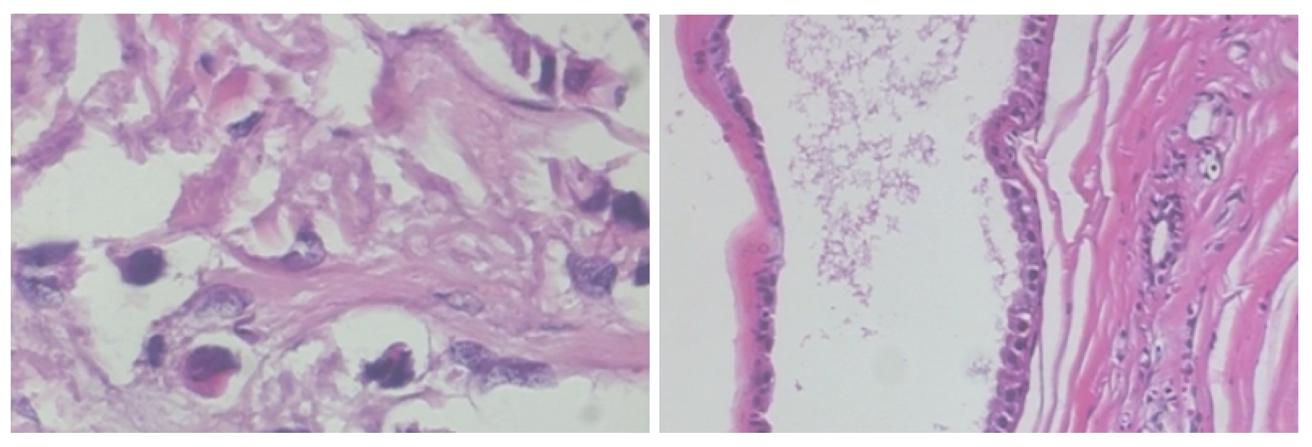
2.1. BreakHis Breast Cancer Histopathological Image Dataset

Our neural networks breast cancer models were created by analyzing the BreaKHis database [27], which contains 7909 tiny histopathological biopsy images of benign and malignant breast tumors. The distribution of images in the BreakHis database is summarized in Table 2. In an IRB-approved study, patients with traces of breast cancer who visited the the P&D, Brazil, between January to December 2014 were recruited. Those who agreed to participate properly consented. Breast tissue biopsy test slides were created by staining the samples with hematoxylin and eosin, prepared for histopathological examination, and marked by pathologists at the P&D Lab. The widely accepted paraffin preparation methodology was utilized. The overall preparation technique incorporates several steps including fixation, dehydration, clearing, infiltration, inserting, and cutting [49]. Lastly, an experienced pathologist diagnosed every case, which was confirmed by correlative tests, such as by utilizing the immunohistochemistry assessment. An Olympus BX-50 magnifying device having a transfer focal point and magnification of 3.3× fixed to a Samsung sophisticated digital camera SCC-131AN was employed to acquire digitized pictures from the breast tissue slides. Images were procured in red, green, and blue channels (RGB) color space (3-byte color depth, 1 byte for every color channel) utilizing amplifying factors of 40×, 100×, 200× and 400× and comparing the variables to target main points of 4×, 10×, 20×, and 40×. Four images—at the four amplification factors: (a) 40×, (b) 100×, (c) 200×, and (d) 400× were generated. Images generated from a single slide of breast tissue containing a malignant tumor (breast cancer) are shown in Figure 1.

2.2. Convolutional Neural Networks (CNNs)

Convolutional neural networks (CNNs) have recently become the best performing neural networks for image analyses and classification. The BoDMCF approach utilizes pre-trained, state-of-the-art CNN models for feature extraction. This section provides a summary of some of the technical details of the CNN architecture. CNNs are in the category of feedforward neural network (FFN) models, where the signal passes within the network without a loop back and can be expressed in Equation (1) [50].
G ( x ) = g H g H 1 g 1 ( x )
where H indicates the number of hidden layers, and g i denotes the function in the matching layer i. The core functional layers in a typical CNN model incorporate activation, fully connected (FC), pooling layers, and a classification layer. The convolutional layer, f, is comprised of various convolutional kernels ( f 1 f y 1 , f y ) where every f y denotes a linear function in the y t h kernel that can be represented by Equation (2)
f y ( x , j ) = u = m m v = n n d = w w w y ( u , v , w ) I ( x u , j v , z w )
The position of the pixel in the input I is denoted by the coordinates ( x , j , z ) , the weight for the y t h kernel is denoted by W y , and the height, width, and depth of the filter is denoted by m, n, and w. The rectified linear unit (ReLU) is a pixel-wise non-linear function, g, known as the activation layer, is represented in Equation (3) [50,51,52].
g ( x ) = max ( 0 , x )
The pooling layer, k, is a layered non-linear down-sampling function designed to repeatedly decrease the feature representation size. The FC layer is considered a variation of the convolutional layer whose kernel has the size 1 × 1. The classification SoftMax layer ( σ ( z ) i = e z i j = 1 K e z j ) is typically added to the last fully connected layer to calculate the probabilities of I i fit into different classes. Figure 2 shows a simple example of a CNN model that is made up of convolutional, ReLU, max-pooling, and FC layers. The first, second, and fifth ReLu layers precede the maximum-pooling layer, which in turn precedes the three FC layers. In order to express max-pooling formally, let Z be a n l × n l × m l tensor. Max-pooling involves determining the maximum value over the element-wise product of subtensor Z k l ( i , j , q ) and filter W , given by Equation (4).
max Z k l ( i , j , q ) W = max a = 1 , 2 , , k b = 1 , 2 , , k c = 1 , 2 , , r z i + a 1 , j + b 1 , q + c 1 l · w a , b , c

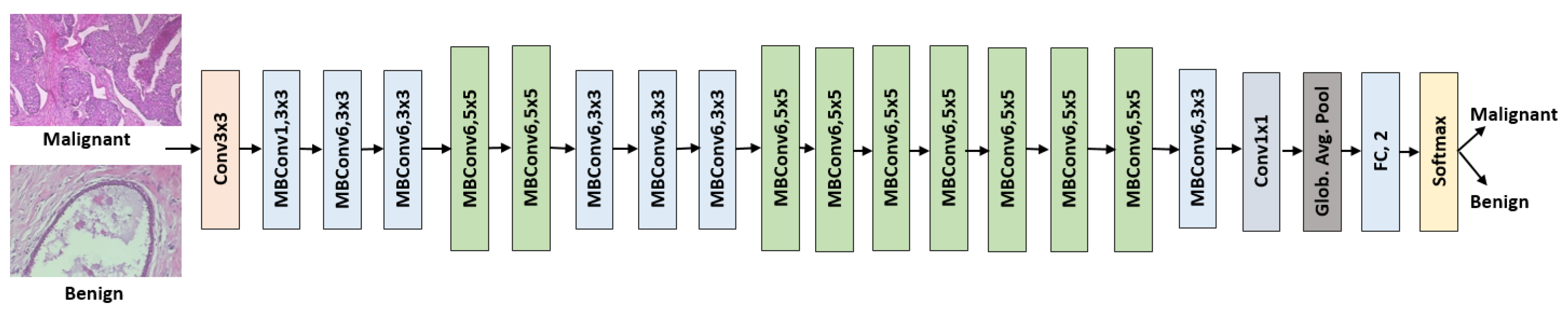
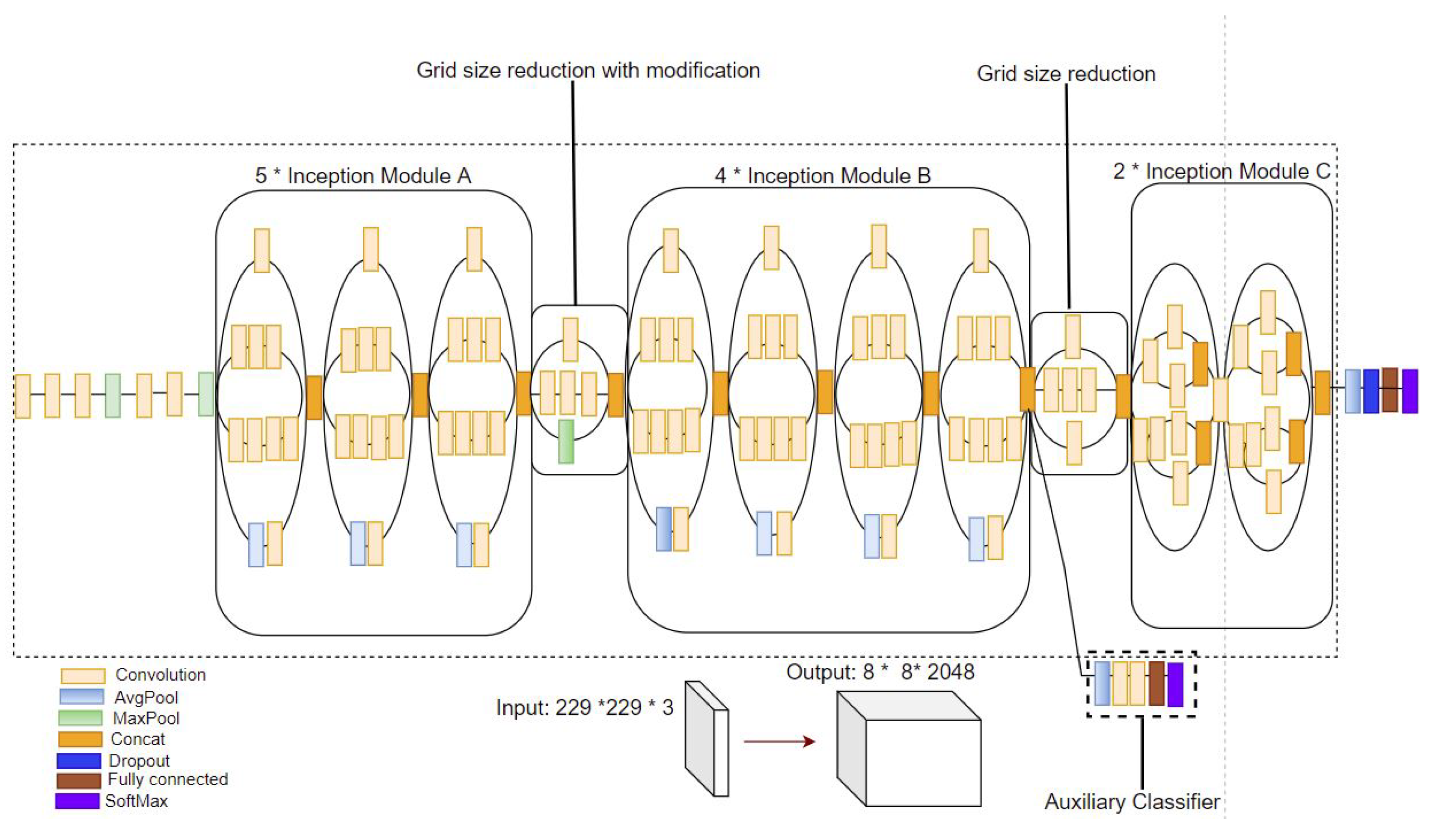
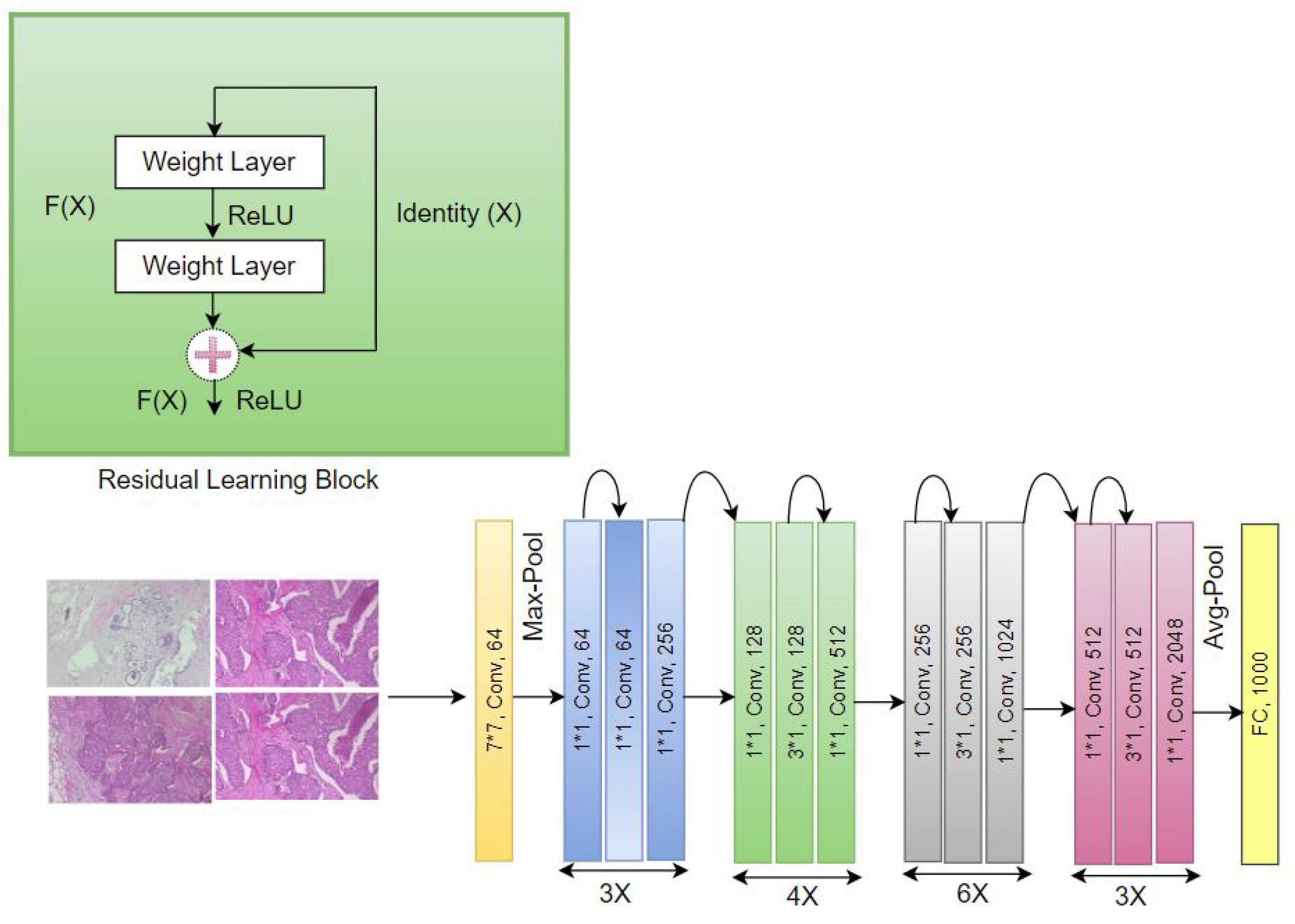
2.3. Pre-Trained CNNs for Deep Image Feature Extraction

To create the bag of deep multi-resolution convolutional features (BoDMCF) representation, features are extracted from four resolutions (40×, 100×, 200× and 400×) of histopathological breast cancer images using three (3) state-of-the-art CNN-based models: (1) (Efficientnet-b0) [17], (2) Inception deep CNN architecture (Inception-v3) [18], (3) ResNet50 [19]. These models were pre-trained on the ImageNet repository that has 14 million images in 1000 categories, enabling them to gain significant intelligence about images [53]. Pre-training is part of a transfer learning approach, which yields higher starting/initial model accuracy during training, faster convergence; and higher asymptotic accuracy (the accuracy level to which the training converges). We now provide some background on these state-of-the-art deep CNN image classification models.
EfficientNet [17]: This architecture and scaling method utilizes a compound coefficient to uniformly scale all depth, width, and resolution dimensions of the CNN using a set of fixed scale coefficients. Given a ConvNet defined as N = i = 1 s F i L i X H i , W i , C i , the EfficientNet architecture can be formulated as an optimization problem given by Equation (5)
max d , w , r Accuracy ( N ( d , w , r ) ) s . t . N ( d , w , r ) = i = 1 s F ^ i d · L ^ i X r · H ^ i , r · W ^ i , w · C ^ i Memory ( N ) target_memory FLOPS ( N ) target_flops
In a principled manner, EfficientNet scales network width, depth, and resolution based on a single δ compound coefficient as expressed in Equation (6).
depth : d = α ϕ width : w = β ϕ resolution : r = γ ϕ s . t . α · β 2 · γ 2 2 α 1 , β 1 , γ 1
For instance, in order to utilize 2N times more computational resources, the network depth can simply be increased by α N , the width by β N , and the image size by γ N , where α , β , and γ are constant coefficients determined by a small grid search on the original small model. In order to capture more fine-grained patterns from a larger input image, the compound scaling method uses more layers to increase the receptive field and more channels to capture a larger number of channels. MobileNet-V2’s [49] inverted bottleneck residual blocks along with squeeze-and-excite blocks are the basis of EfficientNet-B0’s base network. Figure 3 is the architecture for the EfficientNet B0 model.
Inception: This architecture has introduced multiple versions. The first version of the Inception CNN model was introduced as GoogLeNet [54], named Inceptionv1. The enhanced usage of computing resources within the inception1 network is the fundamental feature of this architecture, accomplished by increasing the network’s depth and depth, while sustaining the computational budget. Version 2, also named (Inception-v2), incorporated batch normalization [55]. Version 3 (called Inception-v3) utilized additional factorization ideas [18]. The main distinction of Inception-V3 is that 5 × 5 convolutional layers were used instead of two consecutive layers of 3 × 3 convolutions with up to 128 filters and also the addition of a Batch Norm (BN)-auxiliary. A BN auxiliary is a version of the auxiliary classifier in which the fully connected layer is also normalized in addition to the convolutions. The RMSProp optimizer was also utilized, which has an update rule that can be expressed as:
E g 2 t = β E g 2 t 1 + ( 1 β ) δ C δ w 2 w t = w t 1 η E g 2 t δ C δ w
where E ( g ) is the moving average of squared gradients, ( δ C δ w ) 2 is the gradient of the cost function with respect to the weight, η is the learning rate, and β is the moving average parameter. The classification layers utilized label smoothing regularization (LSR). LSR can be obtained by replacing a single cross entropy H ( q , p ) in the loss function with a pair of losses in the cross entropy, H ( q , p ) and H ( u , p ) , as given in Equation (8) below. The second loss penalizes the deviation of predicted label distribution p from the prior u, with the relative weight ϵ 1 ϵ . H ( u , p ) is a measure of how dissimilar the predicted distribution p is to uniform.
H q , p = k = 1 K log p ( k ) q ( k ) = ( 1 ϵ ) H ( q , p ) + ϵ H ( u , p )
The model is 48 layers deep and capable of classifying images into 1000 image classes, including various object types, keyboard, mouse, pencil, and different animals. This pre-training ensures that the model has gained knowledge of deep high-level feature depictions of an extensive variety of images. Figure 4 is the architecture for the Inception-v3 model.
ResNet: This architecture introduced a deep residual learning structure, which reformulates the CNN’s layers as learning residual functions of the layer inputs. Correctly denoting the desired underlying mapping as K ( i ) , the stacked non-linear layers were made to fit another mapping of E ( i ) : = K ( i ) i . ResNet solved the vanishing gradient, whereby the value of the neural network’s gradient decreases significantly during backpropagation until its weights barely change. ResNet solved the vanishing gradient problem using a skip connection by adding the original input to the output of the convolutional block. A skip connection is a direct connection that skips over some of the model layers and can be expressed as y = F x , W i + W s x , where F x , W i represents the residual mapping to be learned. Resnet utilizes the SGD optimizer with momentum given by Equation (9)
v t = ρ v t 1 + f x t 1 x t = x t 1 α v t
where v t + 1 is the momentum value, ρ is a friction, f x t 1 is the gradient of the objective function at iteration t 1 , x t are parameters, and α is the learning rate. ResNet50 [19], which our approach utilized, is a variant of ResNet. It has 48 convolutional layers and 1 MaxPool layer as well as an average pool layer. Figure 5 is the architecture for the ResNet model.

3. Materials and Methods

Our overall approach involves extracting deep multi-resolution features from four resolutions (40×, 100×, 200× and 400×) of high resolution (2048 × 1536) histopathological breast cancer images using the Efficientnet-b0 [17], Inception-v3) [18], and ResNet50 [19] pre-trained image pre-trained CNN models that are pooled using global pooling to create a BoDMCF. A support vector machine (SVM) classifier then uses the BoDMCF to classify histopathological breast cancer images as either malignant or benign. As shown in Figure 6, the proposed framework of breast cancer classification consists of three main modules: (i) data pre-processing, (ii) deep BoDMCF feature extraction, and (iii) classification using SVM.

3.1. Step 1: Histopathological Image Pre-Processing

During this step, each histopathological image is resized to fit into an input size suitable for different deep CNN models. The histopathological images were resized from 2048 × 1536 to 299 × 299 for inception-v3 and EfficientNet-B0 and to 224 × 224 for resnet-50. Random color data augmentation was also performed on each image by changing the brightness of the image randomly between 50% ( 1 0.5 ) and 150% ( 1 + 0.5 ) of the original image. (See Figure 7) Data augmentation generates diverse samples, which enables the model to learn a robust representation that is invariant to minor changes [56]. Examples of resized histopathological images are shown in Figure 8. After pre-processing, training and test sets were created using a 70:30 split ratio.

3.2. Step 2: Deep Multi-Resolution Feature Extraction Using Pre-Trained CNNs

This stage involves extracting the BoDMCF by modifying the final layers of the three pre-trained deep convolutional networks: Efficientnet-b0, Inception-v3, and ResNet50. These pre-trained models were trained on full-sized ImageNet images, then transfer learning (fine-tuning) was performed on histopathological breast cancer images in our dataset. These feature extractor CNN models utilized layer activations as features. The rich multi-level activations (features) extracted from four resolutions of histopathological images were then pooled to form the BoDMCF and finally used to train a support vector machine (SVM).
EfficientNet [17]: The input size of Efficientnet-b0 was 224 × 224, and Table 3 shows the activation strengths of 56 features learned by the average pooling layer by setting channels to be the vector of indices 1:56 and setting pyramid levels to 3 (three) so that the images are not scaled.
Inception-v3 [18]: The model accepts an image input size of 299 × 299. Table 4 shows the activation strength of 56 features learned by the average pooling layer by setting channels to be the vector of indices 1:56 and setting pyramid levels to 1 (one) so that images are not scaled.
ResNet-50 [19] The input size of ResNet18 is 224 × 224 and Table 5 shows the activation strengths of 56 features learned by the average pooling layer, derived by setting channels to be the vector of indices 1:56 and setting pyramid levels to 1 (one) so that the images are not scaled.

3.3. Step 3: Global Pooling of Features to Create BoDMCF

Features extracted by the three state-of-the-art CNN models (ResNet-50, InceptionV3, and Efficientnet-b0) were pooled to acquire high-quality image descriptions using the activations of the global pooling layers at the end of the network as shown in Figure 9. The network constructs a hierarchical representation of input images. Deeper layers contain higher-level features, constructed using the lower-level features of earlier layers. To obtain the feature representations of the training and test images, activations on the global pooling layer, ‘avg_pool’, at the end of the network are utilized. The global pooling layer pools the input features over all spatial locations, giving 512 features in total as described in Figure 9. For each spatial location, the f activations maps labelled f 1 , f 2 , f 3 , to f 512 are collected, forming 1 × 1 × f column features of dimensions 1,1, 1,2 to h, w. These multiple features are then concatenated into a BoDMCF that is classified using SVM.

3.4. Step 4: BoDMCF Classification Using SVM

SVM was utilized to classify the BoDMCF extracted by the three CNN models as described above. Given a training set and class label ( B n , A n ) , n = 1 , , N , B n R D , A n 1 , 1 , the support vector machine (SVM) classifier [57] tries to find a hyperplane in feature space, which maximizes the margin between two classes (malignant vs. benign). SVM is based on the theory of maximum linear discriminants. For two classes to be classified, SVM finds peripheral data points in each class that are closest to the other class (called support vectors). For a dataset D with n points x i in a d-dimensional space, a hyperplane function h ( x ) can be defined as
h ( x ) = w T x + b = w 1 x 1 + w 2 x 2 + + w d x d + b
Overall, with n points, the margin of the linear classifier can be defined as the minimum distance of a point from the separating hyperplane given as:
δ * = min x i y i w T x i + b w
The SVM classifier finds the optimal hyperplane dividing the two classes by solving the minimization problem with an objective function:
min w i b w 2 2
with linear constraints:
h ( x ) = y i w T x + b 1 , x i D
Then, the class of a new point is predicted as:
y ^ = sign ( h ( z ) ) = sign w T z + b

4. Evaluation and Results

4.1. Evaluation Metrics

The following metrics were used to evaluate all neural networks breast cancer classification models.
Accuracy (Acc): This demonstrates how many malignant cases are correctly predicted and how many benign cases are correctly diagnosed. Equation (15) describes it.
A C C = ( T P + T N ) TP + TN + FP + FN
Sensitivity (Sens): This is the percentage of positive instances correctly predicted, which can be computed using Equation (16).
Sens = T P TP + FN
Precision (Prec): This expresses how many of the positive predictions are actually correct as expressed as Equation (17).
Prec = T P TP + FP
Specificity (Spec): This measures the percentage of correct negative predictions and can be expressed as Equation (18):
Spec = T N TN + FP
F1-score (Fscore): This analyzes sensitivity and precision in harmony by applying a penalty to extreme values in order to reflect their simultaneous impact and can be expressed as Equation (19).
Fscore = T P TP + 1 2 ( FP + FN )
AUC: This is a probability curve that plots the True Postive Rate (TPR) against the False Positive Rate (FPR) at various threshold values and essentially separates the ‘signal’ from the ‘noise’ and is expressed as Equation (20). AUC is a number that ranges from 0 to 1. An AUC value of one indicates a perfect model, while an AUC of 0.5 or below indicates an inadequate model.
A U C = i R i I p I p I p + 1 / 2 I p + I n
where I p and I n denote the number of malignant and benign breast images, respectively, and R i is the rank of the ith positive image in the ranked list.
The Matthews Correlation Coefficient (MCC): This is a contingency matrix metric for calculating the Pearson product-moment correlation coefficient between actual and predicted values that is unaffected by the unbalanced datasets issue. MCC can be expressed as Equation (21).
M C C = T P · T N F P · F N ( T P + F P ) · ( T P + F N ) · ( T N + F P ) · ( T N + F N )
Kappa (Kapp): This is a statistic that compares observed and expected accuracy. It is a measure of how well the instances categorized by a classifier matched the data designated as ground truth. Equation (22) can be used to calculate Kappa.
Kappa = Observed Accuracy Expected Accuracy 1 Expected Accuracy

4.2. Baseline State-of-the-Art CNN Image Classification Architecture
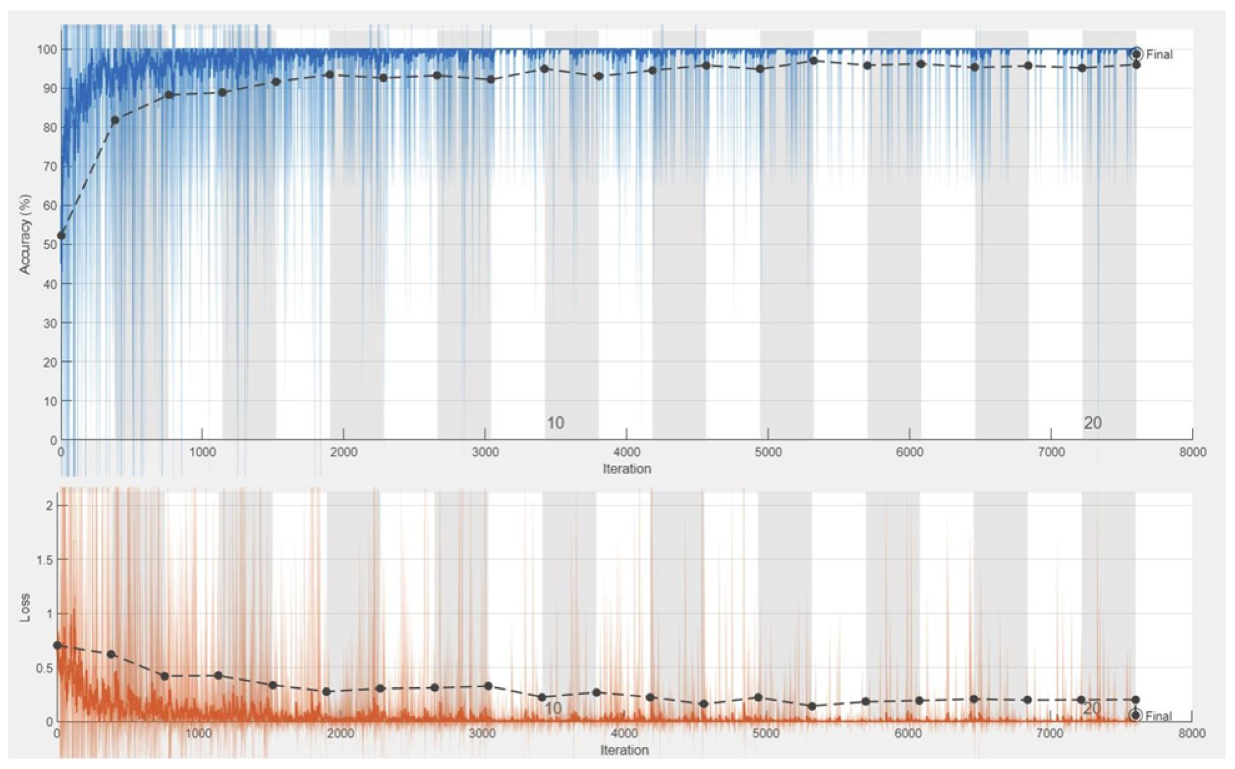
Many of the baseline CNN models we selected for comparison were carefully selected for various reasons, including being winning entries to image analysis and classification competitions and are state of the art and/or performed well on similar problems. They include:
DenseNet201 [58]: This is a 201-layer CNN in which each layer is connected to every other layer in a feedforward manner to eliminate the vanishing gradient problem, enhance feature propagation, promote reuse of features, and drastically reduce the number of parameters. DenseNet is based on the idea that convolutional networks can be more accurate and efficient to train if they have shorter connections between the layers near the input and the layers near the output. We selected DenseNet 201 because it was utilized in prior work [59] as a feature extractor for deep hybrid architectures for binary classification of breast cancer images.
SqueezNet [60]: This is a lightweight CNN that employs various design strategies that reduce the number of parameters, particularly with use of fire modules which “squeeze” parameters using 1 × 1 convolutions for the network to carry fewer parameters. The problem of storage efficiency and speed of models for prediction was solved using a technique known as model compression, which it accomplished by: (i) compressing the perspective of model weight values, and (ii) compressing the perspective of network architecture. SqueezeNet was selected because it was previously utilized for deep feature extraction and classification of breast ultrasound images [61].
ShuffleNet [62]: This is a convolutional neural network specifically designed for mobile devices with low processing power. The architecture uses two new operations, pointwise group convolution and channel shuffle, to reduce computation costs while preserving accuracy. ShuffleNet was selected as a baseline because it was utilized for breast cancer classification in prior work [63].

4.3. Experiments

In this section, experiments to rigorously evaluate our proposed BoDMCF approach using the BreakHis dataset of histopathological breast cancer images [27] that is summarized in Table 2 are described. The classification task was performed by fine-tuning (transfer learning) the CNN models that were previously pre-trained on the ImageNet dataset and on the BreakHis dataset. Various hyperparameters shown in Table 6 were determined using grid search and specified, followed by pre-processing, training, and validation of histopathological images. Test images were then provided as inputs to the trained models. The fine-tuned, pre-trained CNN models were used to extract features at four resolutions, which were pooled to form the BoDMCF that was then classified using SVM. The classifier performance was evaluated with ten-fold cross-validation with a cross-validation error of 0.0462.
Experiment: train-test curves: Figure 10 shows sample train–test curves we generated during training of the EfficientNetb0 model demonstrating model convergence after about 200 epochs.
Experiment: binary classification (benign vs. malignant) of individual magnifications (40×, 100×, 200× and 400×) of histopathological breast cancer images using baseline models with model parameters (weights) determined by pre-training on ImageNet weights: The goal of this experiment was to establish baseline performance of individual state-of-the-art CNN image classification models (ResNet18, InceptionV3, InceptionResnetV2, DenseNet201, ResNet50, EfficientNetB0, SqueezeNet, and ShuffleNet) using weights determined via pre-training on ImageNet (no fine-tuning on the BreakHis dataset). Classification was at individual image resolution with no pooling of features to create the BoDMCF. Our goal was to eventually demonstrate that pooling multiple resolutions of features to create our BoDMCF approach outperforms these powerful baselines that perform classification on single image resolutions. The results of this experiment are shown in Table 7. Except for the precision metric (ResNet18 on 200× magified image hasthe highest precision), SqueezeNet performed best on all other metrics (accuracy, F1 score, recall, AUC, Kappa, and MCC). These results suggest that visual attributes that most clearly distinguish malignant tumors from benign ones are most observable at 100× magnification and that the SqueezeNet neural networks model outperforms all other baseline models when model weights learned from ImageNet during pre-training (no fine-tuning on the BreakHis dataset) are utilized.
Experiment: binary classification (benign vs. malignant) using features extracted from individual magnifications (40×, 100×, 200× and 400×) of histopathological breast cancer images by baseline CNN models fine-tuned on the BreakHis dataset, which are then classified using SVM: The goal of this experiment was to demonstrate the power of pooling multiple resolutions of deep CNN features. Specifically, we benchmarked the performance of deep features extracted at individual magnifications using state-of-the-art fine-tuned CNN image classification models (ResNet18, InceptionV3, InceptionResnetV2, DenseNet201, ResNet50, EfficientNetB0, SqueezeNet, and ShuffleNet) without pooling multiple magnifications into a single BoDMCF representation as we proposed. The results of this experiment are shown in Table 8. Except for the precision metric (ResNet50 on the 40× magnified image has the highest precision), DenseNet201 performed best on all other metrics (accuracy, F1 score, recall, AUC, Kappa, and MCC). These results suggest that when utilized as feature extractors, visual attributes that most clearly distinguish malignant tumors from benign ones are most observable at 40× magnification and that using the DenseNet201 with fine-tuning on the BreakHis dataset outperforms all other baselines as a feature extractor.
Experiment: binary classification (benign vs. malignant) of a combined pool of all four magnifications (40×, 100×, 200× and 400×) of histopathological breast cancer images using baseline models with model parameters (weights) determined by pre-training on ImageNet: The main difference with our proposed approach is that, while all four magnifications were pooled in this experiment, only a single CNN pre-trained model (one of ResNet18, InceptionV3, InceptionResnetV2, DenseNet201, ResNet50, EfficientNetB0, SqueezeNet. and ShuffleNet) was used for classifying the pool of images at a time. In contrast, our proposed approach extracts features using an ensemble of three CNN models (ResNet18, InceptionV3, and ResNetInceptionV2). The results of this experiment are shown in Table 9. Except for the precision metric (DenseNet201 has the highest precision), SqueezeNet performed best on all other metrics (accuracy, F1 score, re- call, AUC, Kappa, and MCC). These results suggest the SqueezeNet neural networks architecture outperforms all other baselines on a multi-resolution bag of features when model weights learned from ImageNet during pre-training are utilized.
Experiment: binary (benign vs. malignant) classifier performance: comprehensive table of metrics for features extracted from a pooled combination of all four magnifications (40×, 100×, 200× and 400×) of histopathological images using baseline CNN models that are classified using SVM The main difference with our proposed approach is that, while all four magnifications were pooled in this experiment, features were extracted using only a single CNN pre-trained model (one of ResNet18, InceptionV3, InceptionResnetV2, DenseNet201, ResNet50, EfficientNetB0, SqueezeNet, and ShuffleNet) at a time. In contrast, our proposed approach extracts features using an ensemble of three CNN models (ResNet18, InceptionV3, and ResNetInceptionV2). The results of this experiment are shown in Table 10. Except for the precision metric (DenseNet50 has the highest precision), EfficientNetB0 performed best on all other metrics (accuracy, F1 score, recall, AUC, Kappa, and MCC). These results suggest the EfficientNetB0 neural networks architecture outperforms all other baselines as a deep feature extractor from a pool of multiple magnifications of histopathological images.
Results of Our BoDMCF approach: Our approach has two key distinctions with the baseline approaches presented thus far. First, we extract features from all four magnifications of histopathological images, which are then pooled into a BoDMCF. Secondly, we use multiple (three) state-of-the-art CNN models (ResNet-50, InceptionV3, and Efficientnet-b0) as feature extractors. The results of our approach, which are shown in Table 10 for individual networks and Table 11, demonstrate that our approach outperforms the baseline approaches. Figure 11 shows samples of test images with their predicted labels from our proposed method. Finally, to demonstrate that the difference in performance between our BoDMCF approach and other ensemble baselines is was statistically significant, we performed the Nemenyi post hoc test [64]. At a confidence level a = 0.05, the critical distance (CD) is 1.2536.
Table 11. Results of our proposed approach with features extracted from all four histopathological image magnifications (40×, 100×, 200× and 400×) by three state-of-the-art CNN models (ResNet-50-, InceptionV3, and EfficientNet-b0). The effects of the number of features used on model performance are also shown. The 2- and 3-model combinations were based on best performing single model performance in Table 9. Accuracy achieved by prior breast cancer binary classification work are also shown in the bottom Table 12.
F. ExtractorsSizeBytesAcc.Sens.Spec.AUCF1-Sc.TPRFPRMCCKappaPrec.
Efficientnetb0 $ Resnet50Train_features 5536 × 3328 Test_features 2373 × 3328Train_features 73,695,232 Test_features 31,589,3760.99660.99870.96620.99720.99460.99870.00430.99220.83780.9907
Efficientnetb0 $ Inception-V3Train_features 5536 × 2816 Test_features 2373 × 2816Train_features 62,357,504 Test_features 26,729,4720.99620.99330.96990.93520.99390.99330.00250.99120.93520.9946
Resnet50 $ Inception-V3Train_features 5536 × 3584 Test_features 2373 × 3584Train_features 79,364,096 Test_features 34,019,3280.99790.99600.97050.99740.99660.99600.00120.99510.83750.9973
BoDMCFTrain_features 5536 × 4864 Test_features 2373 × 4864Train_features 107,708,416 Test_features 46,169,0880.99920.99870.97970.99900.99870.99870.00060.99800.83680.9987
Table 12. Accuracy achieved by prior breast cancer binary classification work are also shown in the bottom table.
AuthorsModelsAccuracy
M. Amrane [14]Naive Bayes (NB) k-nearest neighbor (KNN)97.51% for KNN and 96.19% for NB
S. H. Kassani, M. J. Wesolowski, and K. A. Schneider [29]VGG19, MobileNet, and DenseNet98.13%
F. A. Spanhol, L. S. Oliveira, C. Petitjean, and L. Heutte [31]Ensemble models85.6%
Kowal et al. [32]Deep learning model92.4%
A. Al Nahid, M. A. Mehrabi, and Y. Kong [36]CNN, LSTM, K-means clustering, Mean-Shift clustering and SVM96.0%
Our Proposed ApproachBoDMCF + SVM99.92%
Experiment: ROC Curves The receiver operating characteristic (ROC) curve, shown in Figure 12 for our approach, is a graphical plot that shows the diagnostic ability of a binary classifier as its discrimination threshold is varied. In simple terms, the ROC curve plots our approaches FPR vs. its TPR. The ROC curve is almost a perfect right angle at the top left corner, demonstrating that our proposed approach achieves excellent FPR and TPR.
Experiment: Confusion Matrix: To evaluate which classes were confounded by other classes, we analyzed the confusion matrix. The confusion matrix of the top performing technique is presented in Figure 13. The columns correspond to the targeted class, and the rows correspond to the output class (anticipated class). The diagonal cells match with observations that are rightly classified. The off-diagonal cells refer to incorrect classifications. The percentage of the overall number of observations and the number of observations in every cell is also presented. The column on the extreme right displays the proportions of incorrect (red color) and correct (green color) classifications that were predicted. These metrics are referred to as the false discovery rate and the positive predictive value. While the lowest row indicates the percentages of incorrect and correct classifications, and these metrics are referred to as false negative rate (FNR) and true positive rate (TPR), the cell in the bottom-most right shows the general precision. A column-normalized column summary displays the percentages of incorrectly and correctly classified observations for every predicted class. A row-standardized row summary exhibits the percentages of incorrectly and correctly classified observations for every true class. In the confusion matrix, most of the results fall on the leading diagonal with very few off the diagonal, which demonstrates that the proposed approach did not confuse the benign and malignant classes.
Experiment: classifying the BoDMCF representation using different machine learning classifiers: The goal of this experiment was to compare the performance of the support vector machines (SVM) with other traditional machine learning (ML) classifiers for the task of classifying the BoDMCF representation into target labels of “Benign” and “Malignant”. Results in Table 13 show that SVM outperformed all other ML classifiers for this binary classification task. This is likely because SVM is well-known to perform well on binary classification tasks.
Experiment: CNN model interpretability using grad-cam [65] The goal of this experiment was to ensure that the breast cancer classification model focused on the appropriate regions of the image when analyzing the image. Grad-cam computes the gradient of the ranking score in relation to the CNN characteristics map, highlighting the specific ROIs based on the greatest gradient score. Grad-cam computes the gradients with respect to feature maps of a convolutional layer, which are then global-average-pooled to obtain the importance weights α k c ; α k c represents a partial linearization of the deep network downstream from A, capturing the importance of feature map k for a target class c
α k c = 1 Z i j global average pooling y c A i j k gradients via backprop
y c A i j k is the gradient of the score for class c, y c , with respect to feature maps A k of a convolutional layer. A grad-cam heatmap is then generated as a weighted combination of forward activation feature maps, but followed by a ReLU activation function
L Grad CAM c = Re L U k α k c A k linear combination
where L Grad CAM c is the class-discriminative localization map. Grad-cam was applied to produce a coarse localized map highlighting the most important ROIs in the histopathological images to classify the images as benign or malignant. Sample grad-cam results are shown in Figure 14.
Experiment: analysis of misclassified images: The objective of this experiment was to discover reasons behind model misclassifications, which could be addressed either to improve this manuscript or in future work. Misclassifications resulted for benign images that looked similar to malignant images or vice versa. One example each of misclassified malignant and benign histopathological images, respectively, from the Breakhis dataset is shown in Figure 15. The outline and uniformity of the texture differences in the benign image are comparable to those in a malignant image. There is less dispersion of cells in misclassified malignant images than in ordinary malignant images. Consequently, the cells appear benign, resulting in misclassification. Benign histopathology images usually have fewer dispersed cells and only a few spreads elsewhere.

5. Discussion

Through rigorous experimentation, as shown in Table 11, we demonstrated that the proposed BoDMCF approach outperforms a comprehensive set of baselines as well as the prior state-of-the-art methods (Table 12) for binary classification of histopathological images. Our results also demonstrate that all key components of our approach contribute non-trivially to its superior results, including:
Transfer learning by pre-training on a large image repository (ImageNet) with fine-tuning on the BreakHis breast cancer image dataset that enables the CNN feature extractors models to learn a robust image representation from the large image repository. Fine-tuning on the BreakHis breast cancer dataset transfers the learned intelligence to the task of analyzing and classifying breast cancer. This conclusion is evident by comparing results in Table 7 (pre-training with no fine-tuning) and Table 8 (pre-training with fine-tuning).
Using an ensemble of CNNs for deep feature extractors achieves superior performance to using any single pre-trained CNN for feature extraction, which is evident by comparing results in Table 10 and Table 11. In fact, as shown by the results in Table 11, we also show that the three specific state-of-the-art CNN models (ResNet-50, InceptionV3, and Efficientnet-b0) discovered through extensive experimentation and utilized for feature extraction, outperform other CNN combinations and ensembles. Intuitively, each CNN extracts slightly different image features. Feature extraction using multiple CNNs combines these different features into a superset of features that outperforms features extracted from any single CNN.
Extracting deep features for four magnifications (40×, 100×, 200× and 400×) of histopathological images that are then pooled into a BoDMCF, is important as the visual attributes that distinguish malignant from benign tumors may be most discernable at different resolutions. This conclusion is evident because the results of the pooled, multiresolution BoDMCF features (Table 13) outperform results of classifying deep features extracted from any individual single resolution as shown in Table 8.
Global pooling of multiresolution features to create a bag (BoDMCF0) is an essential step that also enables downstream classification using traditional machine learning algorithms such as SVM. Deep BoDMCFs are a powerful representation, which had the best performance for all combinations of CNN models explored in this study as shown in Table 13. The proposed technique of using BoDMCF features, pooled and classified using SVM, outperformed single CNN model approaches in Table 10.
SVM outperformed all other traditional ML classification algorithms for classifying the BoDMCF into malignant and benign target classes as shown in Table 13. We believe that this is because SVM’s maximal margin hyperplane determination approach performs well on binary classification.
Limitations of this work and potential future work: The results acquired show that very significant classification performance can be achieved. While our proposed approach is shown to perform well on the BreakHis dataset, one of the most widely distributed histopathological images hosted on the public domain, some limitations can be addressed in future work. Firstly, extending the dataset to include more images from more magnifications could yield more robust classifiers before deployment for use in hospitals. Secondly, we used three existing deep models. In future, fusing deeper models could yield better performance. Third, we would like to validate our results on other histopathological breast cancer datasets. Finally, implementing our methods on mobile devices can be a promising direction that facilitates deployment in under-resourced environments such as third world countries.

6. Conclusions

We have proposed an automatic classification method for breast cancer histopathological images into malignant vs. benign categories. Particularly, we have shown that a deep BoDMCF feature extraction from multiple magnifications (40×, 100×, 200× and 400×) of histopathological images using three state-of-the-art pre-trained CNN models (ResNet-50, Inception-v3, and EfficientNet-b0) with pooling and classification using SVM, can also be leveraged for binary (malignant vs. benign) breast cancer classification. Moreover, combining deep rich features from various global average pooling layers of various pre-trained convolutional deep models was shown to yield improved classification performance. In rigorous evaluation experiments, our deep BoDMCF feature approach with global pooling achieved an average accuracy of 99.92% for the classification task, sensitivity of 0.9987, specificity (or recall) of 0.9797, positive prediction value (PPV) or precision of 0.99870, F1-Score of 0.9987, MCC of 0.9980, Kappa of 0.8368, and AUC of 0.9990 on the BreaKHis dataset [27]. Our deep BoMCF approach outperforms state-of-the-art CNN baselines including ResNet18, InceptionV3, DenseNet201, EfficientNetb0, SqueezeNet, and ShuffleNet when classifying any of the individual resolutions (40×, 100×, 200× or 400×) or when SVM is used to classify a BoMCF extracted using any single pre-trained CNN model. The high accuracy, sensitivity, PPV, and F1 score achieved by our approach is extremely encouraging and could be useful in supporting the work of health practitioners in low-resource settings with few experts. However, before deployment, a careful validation study and comparison of our model’s performance to human experts needs to be conducted. In future work, combining several other image magnifications using emerging CNN models could yield even better breast cancer classification models.

Author Contributions

D.C., E.A. and W.S. conceived the presented idea; J.O. and S.A. were involved in the conceptualization and supervision of the research; D.C. and E.A. developed the theory and performed the computations; E.A. and W.S. verified the analytical methods; E.A. and W.S. encouraged D.C. to investigate the algorithm used for this work and supervised the findings of this work. All authors discussed the results and contributed to the final manuscript. All authors have read and agreed to the published version of the manuscript.

Funding

This research received no external funding.

Institutional Review Board Statement

The study utilized a publicly available, de-identified dataset. Hence, IRB approval was not required.

Informed Consent Statement

The study utilized a publicly available, de-identified dataset. Hence, IRB approval and an informed consent was not required.

Data Availability Statement

The study utilized BreakHis, a publicly available, de-identified breast cancer dataset that is available at https:web.inf.ufpr.brvridatabasesbreast-cancer-histopathological-database-breakhis (accessed on 1 October 2022).

Conflicts of Interest

The authors declare no conflict of interest.

References

  1. Siegel, R.L.; Miller, K.D.; Jemal, A. Cancer statistics, 2020. CA. Cancer J. Clin. 2020, 70, 7–30. [Google Scholar] [CrossRef] [PubMed]
  2. Siegel, R.L.; Miller, K.D.; Jemal, A. Cancer statistics, 2019. CA. Cancer J. Clin. 2019, 69, 7–34. [Google Scholar] [CrossRef] [PubMed] [Green Version]
  3. Murtaza, G.; Shuib, L.; Wahab, A.W.A.; Mujtaba, G.; Mujtaba, G.; Nweke, H.F.; Al-garadi, M.A.; Zulfiqar, F.; Raza, G.; Azmi, N.A. Deep learning-based breast cancer classification through medical imaging modalities: State of the art and research challenges. Artif. Intell. Rev. 2019, 53, 1655–1720. [Google Scholar] [CrossRef]
  4. Birdwell, R.L.; Ikeda, D.M.; O’Shaughnessy, K.F.; Sickles, E.A. Mammographic characteristics of 115 missed cancers later detected with screening mammography and the potential utility of computer-aided detection. Radiology 2001, 219, 192–202. [Google Scholar] [CrossRef] [PubMed]
  5. Doi, K. Current status and future potential of computer-aided diagnosis in medical imaging. Br. J. Radiol. 2005, 78, 21–30. [Google Scholar] [CrossRef]
  6. Salama, M.S.; Eltrass, A.S.; Elkamchouchi, H.M. An Improved Approach for Computer-Aided Diagnosis of Breast Cancer in Digital Mammography. In Proceedings of the 2018 IEEE International Symposium on Medical Measurements and Applications (MeMeA), Rome, Italy, 11–13 June 2018; pp. 1–5. [Google Scholar] [CrossRef]
  7. Eldredge, J.D.; Hannigan, G.G. Emerging trends in health sciences librarian. Heal. Sci. Librariansh. 2014, 1, 53–84. [Google Scholar] [CrossRef] [Green Version]
  8. Kasban, H.; El-Bendary, M.A.M.; Salama, D.H. A Comparative Study of Brain Imaging Techniques. Int. J. Inf. Sci. Intell. Syst. 2015, 4, 37–58. [Google Scholar]
  9. He, L.; Long, L.R.; Antani, S.; Thoma, G.R. Histology image analysis for carcinoma detection and grading. Comput. Methods Programs Biomed. 2012, 107, 538–556. [Google Scholar] [CrossRef] [Green Version]
  10. Yan, R.; Ren, F.; Wang, Z.; Wang, L.; Zhang, T.; Liu, Y.; Rao, X.; Zheng, C.; Zhang, F. Breast cancer histopathological image classification using a hybrid deep neural network. Methods 2019, 173, 52–60. [Google Scholar] [CrossRef]
  11. Alarabeyyat, A.; Alhanahnah, M. Breast Cancer Detection Using K-Nearest Neighbor Machine Learning Algorithm. In Proceedings of the 9th International Conference on Developments in eSystems Engineering (DeSE), Liverpool, UK, 31 August–1 September 2016; pp. 35–39. [Google Scholar]
  12. Prabhakar, S.K.; Rajaguru, H. Performance Analysis of Breast Cancer Classification with Softmax Discriminant Classifier and Linear Discriminant Analysis. In Proceedings of the International Conference on Biomedical and Health Informatics, Thessaloniki, Greece, 18–21 November 2017; Maglaveras, N., Chouvarda, I., de Carvalho, P., Eds.; Springer: Singapore, 2018; Volume 66. [Google Scholar]
  13. Asri, M.H.; Moatassime, H.A. Using Machine Learning Algorithms for Breast Cancer Risk Prediction and Diagnosis. Procedia Comput. Sci. 2016, 83, 1064–1073. [Google Scholar] [CrossRef]
  14. Amrane, M.; Oukid, S.; Gagaoua, I.; Ensari, T. Breast cancer classification using machine learning. In Proceedings of the 2018 Electric Electronics, Computer Science, Biomedical Engineerings’ Meeting (EBBT), Istanbul, Turkey, 18–19 April 2018; IEEE: Piscataway, NJ, USA, 2018; pp. 1–4. [Google Scholar]
  15. Shen, D.; Wu, G.; Suk, H.-I. Deep Learning in Medical Image Analysis. Annu. Rev. Biomed. Eng. 2017, 19, 221–248. [Google Scholar] [CrossRef] [PubMed] [Green Version]
  16. Litjens, G.; Kooi, T.; Bejnordi, B.E.; Setio, A.A.A.; Ciompi, F.; Ghafoorian, M.; van der Laak, J.A.W.M.; van Ginneken, B.; Sánchez, C.I. A survey on deep learning in medical image analysis. Med. Image Anal. 2017, 42, 60–88. [Google Scholar] [CrossRef] [PubMed] [Green Version]
  17. Tan, M.; Le, Q. Efficientnet: Rethinking model scaling for convolutional neural networks. In Proceedings of the International Conference on Machine Learning, Long Beach, CA, USA, 10–15 June 2019; pp. 6105–6114. [Google Scholar]
  18. Szegedy, C.; Vanhoucke, V.; Ioffe, S.; Shlens, J.; Wojna, Z. Rethinking the Inception Architecture for Computer Vision. In Proceedings of the IEEE Conference on Computer Vision and Pattern Recognition, Las Vegas, NV, USA, 27–30 June 2016; pp. 2818–2826. [Google Scholar] [CrossRef] [Green Version]
  19. He, K.; Zhang, X.; Ren, S.; Sun, J. Deep residual learning for image recognition. In Proceedings of the IEEE Conference on Computer Vision and Pattern Recognition, Las Vegas, NV, USA, 27–30 June 2016; pp. 770–778. [Google Scholar]
  20. Zheng, B.; Yoon, S.W.; Lam, S.S. Breast cancer diagnosis based on feature extraction using a hybrid of K-means and support vector machine algorithms. Expert Syst. Appl. 2014, 41, 1476–1482. [Google Scholar] [CrossRef]
  21. Yin, F.F.; Giger, M.L.; Doi, K.; Vyborny, C.J.; Schmidt, R.A. Computerized detection of masses in digital mammograms: Automated alignment of breast images and its effect on bilateral-subtraction technique. Med. Phys. 1994, 21, 445–452. [Google Scholar] [CrossRef] [PubMed]
  22. Eltonsy, N.H.; Tourassi, G.D.; Elmaghraby, A.S. A concentric morphology model for the detection of masses in mammography. IEEE Trans. Med. Imaging 2007, 26, 880–889. [Google Scholar] [CrossRef]
  23. Barata, C.; Marques, J.S.; Celebi, M.E. Improving dermoscopy image analysis using color constancy. In Proceedings of the 2014 IEEE International Conference on Image Processing (ICIP), Paris, France, 27–30 October 2014; Volume 19, pp. 3527–3531. [Google Scholar] [CrossRef]
  24. Pinto, A.; Pereira, S.; Correia, H.; Oliveira, J.; Rasteiro, D.M.L.D.; Silva, C.A. Brain Tumour Segmentation based on Extremely Randomized Forest with high-level features. In Proceedings of the 2015 37th Annual International Conference of the IEEE Engineering in Medicine and Biology Society (EMBC), Milan, Italy, 25–29 August 2015; pp. 3037–3040. [Google Scholar] [CrossRef]
  25. Tustison, N.J.; Shrinidhi, K.L.; Wintermark, M.; Durst, C.R.; Kandel, B.M.; Gee, J.C.; Grossman, M.C.; Avants, B.B. Optimal Symmetric Multimodal Templates and Concatenated Random Forests for Supervised Brain Tumor Segmentation (Simplified) with ANTsR. Neuroinformatics 2015, 13, 209–225. [Google Scholar] [CrossRef]
  26. Cheng, G.; Li, Z.; Yao, X.; Guo, L.; Wei, Z. Remote sensing image scene classification using bag of convolutional features. IEEE Geosci. Remote Sens. Lett. 2017, 14, 1735–1739. [Google Scholar] [CrossRef]
  27. Spanhol, F.A.; Oliveira, L.S.; Petitjean, C.; Heutte, L. A Dataset for Breast Cancer Histopathological Image Classification. IEEE Trans. Biomed. Eng. 2016, 63, 1455–1462. [Google Scholar] [CrossRef]
  28. Vaccaro, F.; Bertini, M.; Uricchio, T.; Del Bimbo, A. Image Retrieval using Multi-scale CNN Features Pooling. In Proceedings of the 2020 International Conference on Multimedia Retrieval, Dublin, Ireland, 8–11 June 2020; pp. 311–315. [Google Scholar]
  29. Kassani, S.H.; Kassani, P.H.; Wesolowski, M.J.; Schneider, K.A.; Deters, R. Classification of histopathological biopsy images using ensemble of deep learning networks. arXiv 2019, arXiv:1909.11870. [Google Scholar]
  30. Maqsood, S.; Damaševičius, R.; Maskeliūnas, R. TTCNN: A Breast Cancer Detection and Classification towards Computer-Aided Diagnosis Using Digital Mammography in Early Stages. Appl. Sci. 2022, 12, 3273. [Google Scholar] [CrossRef]
  31. Spanhol, F.A.; Oliveira, L.S.; Petitjean, C.; Heutte, L. Breast Cancer Histopathological Image Classification using Convolutional Neural Networks. In Proceedings of the 2016 International Joint Conference on Neural Networks (IJCNN), Vancouver, BC, Canada, 24–29 July 2016. [Google Scholar]
  32. Kowal, M.; Skobel, M.; Gramacki, A.; Korbicz, J. Breast cancer nuclei segmentation and classification based on a deep learning approach. Int. J. Appl. Math. Comput. Sci. 2021, 31, 85–106. [Google Scholar]
  33. Shen, R.; Yan, K.; Tian, K.; Jiang, C.; Zhou, K. Breast mass detection from the digitized X-ray mammograms based on the combination of deep active learning and self-paced learning. Futur. Gener. Comput. Syst. 2019, 101, 668–679. [Google Scholar] [CrossRef]
  34. Byra, M.; Piotrzkowska-Wroblewska, H.; Dobruch-Sobczak, K.; Nowicki, A. Combining Nakagami imaging and convolutional neural network for breast lesion classification. In Proceedings of the 2017 IEEE International Ultrasonics Symposium (IUS), Washington, DC, USA, 6–9 September 2017; pp. 5–8. [Google Scholar] [CrossRef]
  35. Nejad, E.M.; Affendey, L.S.; Latip, R.B.; Ishak, I.B. Classification of histopathology images of breast into benign and malignant using a single-layer convolutional neural network. ACM Int. Conf. Proc. Ser. 2017, 1313, 50–53. [Google Scholar] [CrossRef]
  36. Al Nahid, A.; Mehrabi, M.A.; Kong, Y. Histopathological breast cancer image classification by deep neural network techniques guided by local clustering. Biomed Res. Int. 2018, 2018, 2362108. [Google Scholar] [CrossRef]
  37. Ogundokun, R.O.; Misra, S.; Douglas, M.; Damaševičius, R.; Maskeliūnas, R. Medical Internet-of-Things Based Breast Cancer Diagnosis Using Hyperparameter-Optimized Neural Networks. Future Internet 2022, 14, 153. [Google Scholar] [CrossRef]
  38. Vogado, L.H.S.; Veras, R.M.S.; Araujo, F.H.D.; Silva, R.R.V.; Aires, K.R.T. Leukemia diagnosis in blood slides using transfer learning in CNNs and SVM for classification. Eng. Appl. Artif. Intell. 2018, 72, 415–422. [Google Scholar] [CrossRef]
  39. Gandomkar, Z.; Brennan, P.C.; Mello-Thoms, C. MuDeRN: Multi-category classification of breast histopathological image using deep residual networks. Artif. Intell. Med. 2018, 88, 14–24. [Google Scholar] [CrossRef]
  40. Han, Z.; Wei, B.; Zheng, Y.; Yin, Y.; Li, K.; Li, S. Breast Cancer Multi-classification from Histopathological Images with Structured Deep Learning Model. Sci. Rep. 2017, 7, 4172. [Google Scholar] [CrossRef] [PubMed]
  41. Wichakam, I.; Vateekul, P. Combining Deep Convolutional Networks for Mass Detection on Digital Mammograms. In Proceedings of the 2016 8th International Conference on Knowledge and Smart Technology (KST), Chiangmai, Thailand, 3–6 February 2016; IEEE: Piscataway, NJ, USA, 2016; pp. 239–244. [Google Scholar]
  42. Devnath, L.; Luo, S.; Summons, P.; Wang, D. Automated detection of pneumoconiosis with multilevel deep features learned from chest X-ray radiographs. Comput. Biol. Med. 2021, 129, 104125. [Google Scholar] [CrossRef]
  43. Devnath, L.; Summons, P.; Luo, S.; Wang, D.; Shaukat, K.; Hameed, I.A.; Aljuaid, H. Computer-Aided Diagnosis of Coal Workers’ Pneumoconiosis in Chest X-ray Radiographs Using Machine Learning: A Systematic Literature Review. Int. J. Environ. Res. Public Health 2022, 19, 6439. [Google Scholar] [CrossRef]
  44. Devnath, L.; Fan, Z.; Luo, S.; Summons, P. Detection and Visualisation of Pneumoconiosis Using an Ensemble of Multi-Dimensional Deep Features Learned from Chest X-rays. Int. J. Environ. Res. Public Health 2022, 19, 11193. [Google Scholar] [CrossRef] [PubMed]
  45. Huynh, B.Q.; Li, H.; Giger, M.L. Digital mammographic tumor classification using transfer learning from deep convolutional neural networks. J. Med. Imaging 2016, 3, 034501. [Google Scholar] [CrossRef] [PubMed]
  46. Zhang, B.; Qi, S.; Monkam, P.; Li, C.; Yang, F.; Yao, Y.D.; Qian, W. Ensemble learners of multiple deep CNNs for pulmonary nodules classification using ct images. IEEE Access 2019, 7, 110358–110371. [Google Scholar] [CrossRef]
  47. Filipczuk, P.; Fevens, T.; Krzyzak, A.; Monczak, R. Computer-aided breast cancer diagnosis based on the analysis of cytological images of fine needle biopsies. IEEE Trans. Med. Imaging 2013, 32, 2169–2178. [Google Scholar] [CrossRef]
  48. George, Y.M.; Zayed, H.H.; Roushdy, M.I.; Elbagoury, B.M. Remote computer-aided breast cancer detection and diagnosis system based on cytological images. IEEE Syst. J. 2014, 8, 949–964. [Google Scholar] [CrossRef]
  49. Subhadra, D. Basic Histology: A Color Atlas & Text. Female Reproductive System. Chapter 17. 2016. Available online: https://www.jaypeedigital.com/book/9789352501786/chapter/ch17 (accessed on 25 July 2022).
  50. Xu, B.; Wang, N.; Chen, T.; Li, M. Empirical Evaluation of Rectified Activations in Convolutional Network. arXiv 2015, arXiv:1505.00853. [Google Scholar]
  51. Kingma, D.P.; Ba, J.L. Adam: A method for stochastic optimization. In Proceedings of the ICLR 2015 3rd International Conference on Learning Representations, San Diego, CA, USA, 7–9 May 2015; pp. 1–15. [Google Scholar]
  52. Brown, M.J.; Hutchinson, L.A.; Rainbow, M.J.; Deluzio, K.J.; de Asha, A.R. A comparison of self-selected walking speeds and walking speed variability when data are collected during repeated discrete trials and during continuous walking. J. Appl. Biomech. 2017, 33, 384–387. [Google Scholar] [CrossRef]
  53. Deng, J.; Dong, W.; Socher, R.; Li, L.J.; Li, K.; Fei-Fei, L. Imagenet: A large-scale hierarchical image database. In Proceedings of the 2009 IEEE Conference on Computer Vision and Pattern Recognition, Miami, FL, USA, 20–25 June 2009; IEEE: Piscataway, NJ, USA, 2009; pp. 248–255. [Google Scholar]
  54. Szegedy, P.S.C.; Liu, W.; Jia, Y. Going Deeper with Convolutions. In Proceedings of the IEEE Conference on Computer Vision and Pattern Recognition, Long Beach, CA, USA, 15–20 June 2019; pp. 163–182. [Google Scholar] [CrossRef]
  55. Ioffe, S.; Szegedy, C. Batch normalization: Accelerating deep network training by reducing internal covariate shift. In Proceedings of the 32nd International Conference on Machine Learning, Lille, France, 6–1 July 2015; Volume 1, pp. 448–456. [Google Scholar]
  56. Xiao, Y.; Decencière, E.; Velasco-Forero, S.; Burdin, H.; Bornschlögl, T.; Bernerd, F.; Warrick, E.; Baldeweck, T. A new color augmentation method for deep learning segmentation of histological images. In Proceedings of the 2019 IEEE 16th International Symposium on Biomedical Imaging (ISBI 2019), Venice, Italy, 8–11 April 2019; IEEE: Piscataway, NJ, USA, 2019; pp. 886–890. [Google Scholar]
  57. Hearst, M.A.; Dumais, S.T.; Osuna, E.; Platt, J.; Scholkopf, B. Support vector machines. IEEE Intell. Syst. Their Appl. 1998, 13, 18–28. [Google Scholar] [CrossRef]
  58. Huang, G.; Liu, Z.; Van Der Maaten, L.; Weinberger, K.Q. Densely connected convolutional networks. In Proceedings of the IEEE Conference on Computer Vision and Pattern Recognition, Honolulu, HI, USA, 21–26 July 2017; pp. 4700–4708. [Google Scholar]
  59. Zerouaoui, H.; Idri, A. Deep hybrid architectures for binary classification of medical breast cancer images. Biomed. Signal Process. Control 2022, 71, 103226. [Google Scholar] [CrossRef]
  60. Iandola, F.N.; Han, S.; Moskewicz, M.W.; Ashraf, K.; Dally, W.J.; Keutzer, K. SqueezeNet: AlexNet-level accuracy with 50x fewer parameters and <0.5 MB model size. arXiv 2016, arXiv:1602.07360. [Google Scholar]
  61. Singh, J.; Thakur, D.; Ali, F.; Gera, T.; Kwak, K.S. Deep feature extraction and classification of android malware images. Sensors 2020, 20, 7013. [Google Scholar] [CrossRef] [PubMed]
  62. Zhang, X.; Zhou, X.; Lin, M.; Sun, J. Shufflenet: An extremely efficient convolutional neural network for mobile devices. In Proceedings of the IEEE Conference on Computer Vision and Pattern Recognition, Salt Lake City, UT, USA, 18–23 June 2018; pp. 6848–6856. [Google Scholar]
  63. Aljuaid, H.; Alturki, N.; Alsubaie, N.; Cavallaro, L.; Liotta, A. Computer-aided diagnosis for breast cancer classification using deep neural networks and transfer learning. Comput. Methods Programs Biomed. 2022, 223, 106951. [Google Scholar] [CrossRef] [PubMed]
  64. Nemenyi, P.B. Distribution-Free Multiple Comparisons. Ph.D. Thesis, Princeton University, Princeton, NJ, USA, 1963. [Google Scholar]
  65. Selvaraju, R.R.; Cogswell, M.; Das, A.; Vedantam, R.; Parikh, D.; Batra, D. Grad-cam: Visual explanations from deep networks via gradient-based localization. In Proceedings of the IEEE International Conference on Computer Vision, Venice, Italy, 22–29 October 2017; pp. 618–626. [Google Scholar]
Figure 1. Sample histopathological images. The top row shows benign images at 40×, 100×, 200× and 400× (left to right). The bottom row shows malignant images at 40×, 100×, 200× and 400× (left to right).
Informatics 09 00091 g001
Figure 2. The architecture of a convolutional neural network (CNN).
Informatics 09 00091 g002
Figure 3. EfficientNet B0 CNN architecture.
Informatics 09 00091 g003
Figure 4. Inception-V3 CNN architecture.
Informatics 09 00091 g004
Figure 5. Resnet-50 CNN architecture.
Informatics 09 00091 g005
Figure 6. Our proposed approach: A bag of multiresolution CNN features (BoDMCF) are extracted from multiple resolutions of samples of malignant and benign histopathological images, which are then classified using a support vector machine (SVM) classifier.
Informatics 09 00091 g006
Figure 7. Example of brightness data augmentation operations (left = original, middle = brightness + 50, right = brightness + 150).
Informatics 09 00091 g007
Figure 8. Examples of images after resizing to dimensions 224 × 224 × 3.
Informatics 09 00091 g008
Figure 9. Feature pooling approach to create bag of deep multiresolution convolutional features (BoDMCF).
Informatics 09 00091 g009
Figure 10. Efficientnetbo train-test performance. The small difference between the training and test loss curves demonstrate that there is no overfitting.
Informatics 09 00091 g010
Figure 11. Four sample test images with their predicted labels from our proposed algorithm.
Informatics 09 00091 g011
Figure 12. ROC Curves for our Approach.
Informatics 09 00091 g012
Figure 13. Confusion matrix displaying the performance of the proposed BoDMCF approach.
Informatics 09 00091 g013
Figure 14. Sample heatmaps of regions of interest generated by grad-cam (left pair = malignant original image and grad-cam heatmap, right pair = benign original image and grad-cam heatmap.
Informatics 09 00091 g014
Figure 15. Sample misclassified images. Left is a misclassified malignant image, and right is a misclassified benign image.
Informatics 09 00091 g015
Table 1. Related Work on deep learning and CNNs for breast cancer tumor classification.
AuthorsModelsML ProblemSummary of ApproachAccuracy
R. Yan et al. [10]CNN and RNNFour-class classification into malignant and benign subtypesA CNN was used to extract image patches. Then an RNN was used to fuse the patch features and make the final image classification.91.3%
M. Amrane [14]Naive Bayes (NB) and k-nearest neighbor (KNN)Binary classification (malignant or benign)For NB, data was split into blocks of 2 classes and 2 sets of features T and classes D and statistical analysis were performed. K-nearest neighbor, pick an instance from the testing sets and calculate its distance with the training set.97.51% for KNN and 96.19% for NB
S. H. Kassani, M. J. Wesolowski, and K. A. Schneider [29]VGG19, MobileNet, and DenseNet.Binary classification (malignant or benign)Ensemble model was used for the feature extraction. Then classification was done using a Multi-Layer Perceptron (MLP) classifier98.13%
F. A. Spanhol, L. S. Oliveira, C. Petitjean, and L. Heutte [31]Ensemble modelsBinary classification (malignant or benign)Various CNNs were using a fusion rule for breast cancer classification85.6%
Kowal et al. [32]Deep learning modelBinary classification (malignant or benign)Segmentation, feature extraction and classification were performed on individual cell nuclei of cytological images.92.4%
A. Al Nahid, M. A. Mehrabi, and Y. Kong [36]CNN, LSTM, K-means clustering, Mean-Shift clustering and SVMBinary classification (malignant or benign)A set of biomedical breast cancer images were classified using novel DNN models guided by an unsupervised clustering method96.0%
Z. Gandomkar, P. C. Brennan, and C. Mello-Thoms [39]Deep residual network (ResNet)Multi class classification into Subtypes of malignant and benignApproach consisted of two stages. In the first stage, ResNet layers classified patches from the images as benign or malignant. In the second statge, images were classified into subtypes of malignant and benign98.52%, 97.90%, 98.33%, and 97.66% in 40×, 100×, 200× and 400× magnification factors respectively
Table 2. Distribution of the histopathological breast cancer images in the BreakHis dataset by amplication factor and class.
MagnificationMalignantBenignTotal
40×1370 (68.67%)652 (32.68%)1995
100×1437 (69.05%)644 (30.95%)2081
200×1390 (69.05%)623 (30.94%)2013
400×1232 (67.69%)588 (32.31%)1820
Total 5429 (68.64%)2480 (31.14%)7909
Table 3. Activation strength on 56 features learned by the average pooling layer for efficientNet.
IterationActivation StengthPyramid Level
10.351
20.311
30.591
41.191
51.871
62.561
73.121
83.561
93.871
104.151
Table 4. Activation strength of 56 features learned by the average pooling layer for Inception-V3.
IterationActivation StrengthPyramid Level
10.321
20.351
30.581
40.981
51.511
61.941
72.371
82.731
93.091
103.291
Table 5. Activation strength on 56 features learned by the average pooling layer for ResNet-18.
IterationActivation StrengthPyramid Level
10.941
21.181
32.921
45.341
57.221
68.501
79.411
810.041
910.601
1010.881
Table 6. Optimal hyperparameters used for pre-trained models.
HyperparameterValue
Train-Test ratio70:30
optimization algorithmstochastic gradient descent
activation functionReLu
Mini Batch Size20
Max Epochs30
Initial Learn Rate0.00125
Learn-Rate Drop Factor0.1
Learn-Rate Drop Period20
Table 7. Binary (benign vs. malignant) classifier performance: comprehensive table of metrics for classifying various magnification levels of histopathological images using baseline CNN models with pre-trained weight from ImageNet (no fine-tuning of weights on the BreakHis dataset).
ModelAccuracyPrecisionF1-ScoreRecallAUCKappaMCC
40× Renent180.90640.80470.86070.92510.91150.86670.7950
40× InceptionResnetV20.78430.60210.72610.91440.81970.69240.5937
40× InceptionV30.86790.84180.77100.71120.82520.82470.6839
40× Densenet2010.89630.94330.81100.71120.84590.86290.7555
40× Resnet500.93810.92610.89810.87170.92000.91350.8545
40× Efficientnetbo0.83110.73890.72480.71120.79840.77490.6033
40× Squeezenet0.92810.84290.89170.94650.93310.89700.8413
40× Shufflenet0.84280.82520.71520.63100.78510.79720.6197
100× Renent180.93270.89950.89010.88080.91840.90600.8417
100× InceptionResnetV20.81730.75820.67050.60100.75760.76690.5535
100× InceptionV30.90220.93420.82320.73580.85630.87010.7673
100× Densenet2010.91830.93290.85710.79270.88360.88920.8056
100× Resnet500.91190.86700.85560.84460.89330.87830.7924
100× Efficientnetbo0.85260.83010.73410.65800.79890.80870.6422
100× Squeezenet0.94550.86300.91750.97930.95480.92160.8809
100× Shufflenet0.86060.74540.78730.83420.85330.80750.6865
200× Renent180.87910.98310.76070.62030.80780.84600.7178
200× InceptionResnetV20.86920.90300.75390.64710.80790.83130.6853
200× Inceptionv30.89570.90790.81420.73800.85220.86110.7504
200× Densenet2010.88910.90000.80120.72190.84300.85310.7340
200× Resnet500.86420.75610.79080.82890.85450.81280.6922
200× Efficientnetbo0.82450.73960.70220.66840.78150.77040.5798
200× Squeezenet0.92050.90170.86670.83420.89670.89070.8114
200× Shufflenet0.85260.84510.72950.64170.79450.80990.6421
400× Renent180.86810.91270.76160.65340.81180.82730.6918
400× InceptionResnetV20.81680.72620.70930.69320.78440.75450.5760
400× InceptionV30.72530.54220.69010.94890.78390.59880.5351
400× Densenet2010.86260.86860.76040.67610.81370.81830.6765
400× Resnet500.88460.91850.79740.70450.83740.84600.7311
400× Efficientnetbo0.82780.69710.75520.82390.82680.75850.6290
400× Squeezenet0.92310.95240.79470.68180.83280.84990.7383
400× Shufflenet0.87360.93500.76920.65340.81590.83460.7068
Table 8. Binary (benign vs. malignant) classifier performance: comprehensive table of metrics for deep features extracted from different individual magnifications of histopathological images using fine-tuned CNN models that are classified using SVM (no pooling of features to create a bag (BoDMCF).
ModelAccuracyPrecisionF1-ScoreRecallAUCKappaMCC
40× Resnet180.90640.86190.84780.83420.88670.87060.7804
40× InceptionResnetV20.92140.87230.87460.87700.90930.88990.8174
40× InceptionV30.93480.93530.89080.85030.91180.90950.8464
40× Densenet2010.96150.94090.93830.93580.95450.94510.9104
40× Resnet500.95480.95460.92570.89840.93950.93640.8941
40× Efficientnetbo0.94480.93260.90960.88770.92930.92250.8705
40× Squeezenet0.83950.73010.74960.77010.82050.78170.6324
40× Shufflenet0.87460.81460.79450.77540.84760.82970.7048
100× Renent180.91990.87430.86980.86530.90480.88870.8119
100× InceptionResnetV20.90060.84660.83770.82900.88090.86340.7662
100× InceptionV30.90220.87430.83380.79690.87290.86710.7663
100× Densenet2010.91510.87630.86020.84460.89560.88280.7995
100× Resnet500.93910.88940.90310.91710.93300.91400.8589
100× Efficientnetb00.92950.88210.88660.89120.91890.90120.8355
100× Squeezenet0.85420.77130.76120.75130.82580.80410.6563
100× Shufflenet0.90220.85110.83990.82900.88200.86570.7697
200× Renent180.89400.80900.83420.86100.88490.85270.7572
200× InceptionResnetV20.94210.90000.90720.91440.93440.91820.8651
200× InceptionV30.89900.86630.83010.79680.87080.86270.7598
200× Densenet2010.94000.89890.87670.85560.90620.89680.8239
200× Resnet500.93380.90160.89190.88240.91960.90750.8443
200× Efficientnetbo0.94370.90480.90960.91440.93560.92060.8687
200× Squeezenet0.90560.83850.84960.86100.89330.86890.7810
200× Shufflenet0.90400.88170.83710.79680.87440.86950.7712
400× Renent180.85160.78110.76520.75000.82500.79770.6571
400× InceptionResnetV20.86630.81600.78470.75570.83730.81760.6890
400× InceptionV30.90110.84660.84660.84660.88680.86090.7736
400× Densenet2010.89000.86500.83190.80110.87080.85550.7575
400× Resnet500.91760.86590.87320.88070.90790.88280.8123
400× Efficientnetbo0.91760.85030.90340.87600.91390.88190.8152
400× Squeezenet0.86260.79190.78510.77840.84060.81090.6842
400× Shufflenet0.88280.81110.82020.82950.86880.83590.7334
Table 9. Binary (benign vs. malignant) classifier performance: comprehensive table of metrics for classifying a combined pool of all histopathological image magnifications (40×, 100×, 200× and 400×) extracted using a single state-of-the-art baseline CNN model.
ModelAccuracyPrecisionF1-ScoreRecallAUCKappaMCC
Renent180.88960.93820.79750.69350.83630.85480.7396
InceptionResnetV20.86090.84050.75590.68680.81360.81690.6666
InceptionV30.88450.92110.78960.69090.83190.84820.7262
Densenet2010.91660.95350.85290.77150.87720.88720.8043
Resnet500.90480.89600.83830.78760.87290.87040.7745
Efficientnetb00.82810.85900.66340.54030.74990.78570.5827
Squeezenet0.94600.91950.92010.92070.94190.92870.8835
Shufflenet0.86430.88790.75000.64920.80590.82410.6752
Table 10. Binary (benign vs. malignant) classifier performance: comprehensive table of metrics for features extracted from a pooled combination of all four magnifications (40×, 100×, 200× and 400×) of histopathological images using baseline CNN models that are classified using SVM.
ModelAccuracySensitivityAUCFscoreTPRFPRMCCKappaPrecSpec
Densenet2010.98150.96770.97770.97040.96770.01230.95690.84580.97300.9877
Resnet500.98990.98920.98970.98400.98920.00980.97660.84100.97870.9902
Efficientnetb00.98360.97180.98040.97370.97180.01100.96180.84470.97570.9890
InceptionResnetV20.98230.98660.98350.97220.98660.01960.95940.84390.95820.9804
InceptionV30.98360.97980.98260.97390.97980.01470.96200.84400.96810.9853
Renent180.97770.97980.97830.96490.97980.02330.94880.84610.95050.9767
Shufflenet0.97940.96910.97660.96710.96910.01600.95210.84640.96520.9840
Squeezenet0.96590.96640.96600.94670.96640.03440.92200.85120.92770.9656
Table 13. Results of classifying the BoDMCF with various machine learning (ML) classifiers.
ML ClassifierAcc.Sens.Spec.AUCF1TPRFPRMCCKappaPrec.
Binary Decision Classifier0.96600.94490.97610.96050.94620.94490.02390.92160.85290.9474
Linear Discriminant Analysis (LDA)0.99000.98920.99020.98970.98400.98920.00980.97660.84100.9787
Generalized Additive Model0.96600.94890.97420.96160.94640.94890.02580.92180.85260.9439
Gradient Boosted Machines (GBM)0.98700.98120.98900.98510.97860.98120.01100.96870.84290.9759
K-Nearest Neighbor (KNN)0.98000.99600.97240.98420.96860.99600.02760.95450.84400.9427
Naive Bayes (NB)0.97300.99190.96380.97790.95780.99190.03620.93880.84680.9260
Support Vector Machines (SVM)0.99920.99870.97970.99900.99870.99870.00060.99800.83680.9987
Publisher’s Note: MDPI stays neutral with regard to jurisdictional claims in published maps and institutional affiliations.

