Article

Searching Deterministic Chaotic Properties in System-Wide Vulnerability Datasets

by
Ioannis Tsantilis
1,
Thomas K. Dasaklis
2,*,
Christos Douligeris
1 and
Constantinos Patsakis
1,3
1
Department of Informatics, University of Piraeus, 80 Karaoli & Dimitriou Str., 18534 Piraeus, Greece
2
School of Social Sciences, Hellenic Open University, Aristotelous 18, 26335 Patra, Greece
3
Athena Research Center, Information Management Systems Institute, Artemidos 6, 15125 Marousi, Greece
*
Author to whom correspondence should be addressed.
Informatics 2021, 8(4), 86; https://doi.org/10.3390/informatics8040086
Submission received: 13 September 2021 / Revised: 22 November 2021 / Accepted: 30 November 2021 / Published: 4 December 2021
(This article belongs to the Special Issue Feature Paper in Informatics)

Abstract

:
Cybersecurity is a never-ending battle against attackers, who try to identify and exploit misconfigurations and software vulnerabilities before being patched. In this ongoing conflict, it is important to analyse the properties of the vulnerability time series to understand when information systems are more vulnerable. We study computer systems’ software vulnerabilities and probe the relevant National Vulnerability Database (NVD) time-series properties. More specifically, we show through an extensive experimental study based on the National Institute of Standards and Technology (NIST) database that the relevant systems software time series present significant chaotic properties. Moreover, by defining some systems based on open and closed source software, we compare their chaotic properties resulting in statistical conclusions. The contribution of this novel study is focused on the prepossessing stage of vulnerabilities time series forecasting. The strong evidence of their chaotic properties as derived by this research effort could lead to a deeper analysis to provide additional tools to their forecasting process.

1. Introduction

Cyber attacks against information systems have considerably increased during the recent years. In most cases, the attackers take advantage of a series of system-wide vulnerabilities that are present in operating systems, servers, and other software. A software vulnerability is defined as “a defect which enables an attacker to bypass security measures” [1]. Software vulnerabilities present serious security risks for computing systems. Consequently, the number of undiscovered vulnerabilities in a computing system may have a detrimental impact on its functions and overall operation [2]. The situation is even more crucial for Information Systems (IS) operating in critical infrastructures. In most cases, due to their nature, these systems are far more complex than typical enterprise IS. This complexity stems from many reasons, such as the number of sub-systems they are composed of, their location, and the usually very strict requirements regarding their uptime, availability, and response.
There has always been a trend in various scientific sectors to use statistical forecasting [3,4] (in addition to other mathematical methods) to extract valuable information from the available underlying data samples [5,6]. The security domain seems to have adopted this trait of thought to a certain extent regarding vulnerability data analysis since this method can reveal many hidden patterns in the underlying data [7]. The simplest metric may be the total number of vulnerabilities reported per product based on historically reported security vulnerabilities [8]. Nevertheless, for this metric to be accurate, there is a need for a baseline dataset that lists vulnerabilities and their characteristics. Perhaps one of the most comprehensive datasets of known vulnerabilities is the National Vulnerability Database https://nvd.nist.gov/ (accessed on 6 September 2021) (NVD) hosted and maintained by the National Institute of Standards and Technology (NIST). In particular, NVD keeps track of all the publicly known vulnerabilities since 1998 with their target, scope, publication data, and Common Vulnerability Scoring System (CVSS) score along with other details in a standardised manner [9].

1.1. Motivation and Contribution

The research literature used the patterns discovery approach in vulnerability time series regarding forecasting properties, focusing mainly either on the so-called Vulnerability Discovery Model (VDM) approaches [5,6,10,11,12,13,14,15,16,17,18] or on the Time Between Vulnerability Disclosure (TBVD) [8]. However, limited attention has been paid so far in the literature to severity forecasting of specific IT components [19,20,21,22,23]. It should also be noted that the existing severity-related models (including linear, non-linear and stochastic models), apart from being limited in number, also present limited performance characteristics. It seems that modeling such datasets and time series is incomplete, and a further analysis is required regarding their predictive capacity. Apart from the limited number of severity-related models and their poor performance, another gap in the literature relates to whether the overall assessment focuses on specific components or on the computer systems software. In particular, NVD datasets are used by all researchers in the field of security for discovering patterns in the relevant data. Unfortunately, these datasets consider specific components over time. Therefore, it would be of great interest to discover patterns when considering integrated computer systems comprised of such software components.
This paper addresses these gaps in the literature by applying an extended analysis to discover a variety of properties of the time series mentioned above concerning severity forecasting based on chaos theory. We also demonstrate the feasibility of unravelling system-wide vulnerabilities and not only specific software components vulnerabilities. To this end, we define and study computer systems software vulnerabilities and probe the relevant NVD time-series properties. Based on an extensive experimental analysis of the NIST databases, we showcase that the relevant systems software time series present significant chaotic properties. Moreover, we define systems based on open and closed source software and compare their chaotic properties resulting in a variety of statistical conclusions. The contribution of this novel study highlights that (a) the associated time series are not fully predictable, and (b) the chaotic properties of the available data sets could lead to a deeper investigation to improve risk management assessment of the associated systems. This chaotic nature justifies the poor prediction results of previous works and relevant methods, since they are not the proper ones for this kind of systems. To the best of our knowledge, this is the first paper to report the chaotic properties of this dataset. As a result, the probabilistic analysis of these results indicates that the prediction of vulnerability scores using a time series of vulnerability data is a promising approach with far-reaching implications for adopting proper security management measures.

1.2. Paper Structure

The rest of the paper is organised as follows. Section 2 reviews the related work published in the area of vulnerability disclosure and chaos theory applications. In Section 3, the problem description is defined. In Section 4, we introduce the data collection and processing methodology to create a framework for the analysis of the chaotic properties of the time series. Moreover, it is illustrated how the proposed methodology could be used to measure the properties of a real-world computing system. In Section 5, the empirical framework for the experimental analysis of the chaotic properties of the vulnerability time series is outlined. In Section 6, the results derived by the suggested methodology are evaluated and thoroughly discussed. Finally, the last section summarises the contributions of the proposed methodology and outlines possible further extensions of this work.

2. Literature Review

A significant body of scientific literature, both of qualitative [24] and of quantitative nature [5,13,25,26,27,28], has been produced so far addressing issues of vulnerability forecasting for major operating systems. The aforementioned literature can be classified into two broad categories: (a) statistical-based approaches, in which future vulnerabilities may be found by analysing historically reported vulnerabilities of operating systems and (b) code-specific approaches, in which the predictive capacity of the proposed vulnerability forecasting models rely on the characteristics and attributes of the potentially vulnerable software, its development process, or its source code. Both categories present significant heterogeneity in terms of objectives, methodologies applied and underlying assumptions.
Statistics-based approaches are built using historical vulnerability data, particularly data provided by NVD [8,29]. The benefits of these models rely on the fact that they may forecast vulnerabilities in software for which no detailed information is available (such as the source code). At their core, the bulk of these studies use cumulative regression type approaches, such as VDM approaches, establish statistical forecasting and mathematical models [6,11,16,17,18,26,30,31,32,33]. VDMs are probabilistic models based on parametric mathematical functions counting the number of cumulative vulnerabilities of a particular software at an arbitrary time period [34].
Code-specific approaches are based on various methods for predicting possible system vulnerabilities, such as using machine learning and neural networks [9,35,36,37,38,39,40]. Some authors apply hybrid approaches in which machine learning is combined with regression analysis for developing robust VDM approaches [41,42]. Other studies on vulnerability prediction are based on text mining (with models using software metrics as predictors) [43,44], software-network graphs [45] and multi-criteria decision making approaches based on analytic network processes [46]. A significant body of studies proposes the development of vulnerability discovery prediction models based on code properties and relevant software metrics [47,48,49,50,51,52,53]. It should be noted that the usefulness of the aforementioned studies (the ones based on code properties and software metrics) is limited to open-source software.
An important aspect of the vulnerability forecasting models is the notion of severity. Recent studies have highlighted the importance of taking into account the severity of potential system-wide exploits for developing sound vulnerability forecasting models [19,20,21,22,23,54,55]. It should be noted that the aforementioned approaches, although significant, have not thoroughly explored severity prediction and the exploitation of NVD data using regression models, since this aspect has been recently considered.
Chaos theory is a field of science focused on unpredictability. Using this theory, we are equipped with tools to explore the unexpected, and we can be highly efficient in modeling the behavior of nearly unpredictable complex nonlinear systems. There are numerous applications of chaotic theoretic analysis in physics, biology, chemistry, and engineering [56,57]. Among the always increasing application cases are weather patterns, biological systems, food chains, financial markets, and brain states [58,59]. The examples where chaos is present are widespread, which renders the chaos framework applicable to broad and interdisciplinary areas of study. Moreover, chaos theory has been shown to be an important tool for forecasting in complex dynamical systems [60,61]. Chaos theory could possibly help to understand the security properties of the IT networks/systems and attack properties. Besides understanding security properties, chaotic theory-based analysis could be important in predicting security risks. The goal of the present study is to understand the chaotic properties in NVD in order to be able to provide, in the near future, methodologies for short term risk forecasting in the same line of research as in [60,61]. However, to the best of our knowledge, there is no similar research effort so far for introducing this type of analysis in the investigation of patterns in the vulnerability data. The only exception in the IT domain are works such as [62,63,64] where chaos theory is applied for forecasting network traffic anomalies, which are not related to software vulnerabilities.
An important issue in the research on chaotic systems is the definition of such systems. Although no universally accepted mathematical definition of chaos exists, the following properties should be present for classifying a dynamical system as chaotic [65]:
  • It must be sensitive to the initial conditions
  • It must be topologically transitive
  • It must have dense periodic orbits.
For detecting the presence of such properties in dynamic systems, several metrics have been proposed. The most widely used are Largest Lyapunov exponents (LLEs), Hurst coefficients, and entropy-based measures.

3. Problem Description
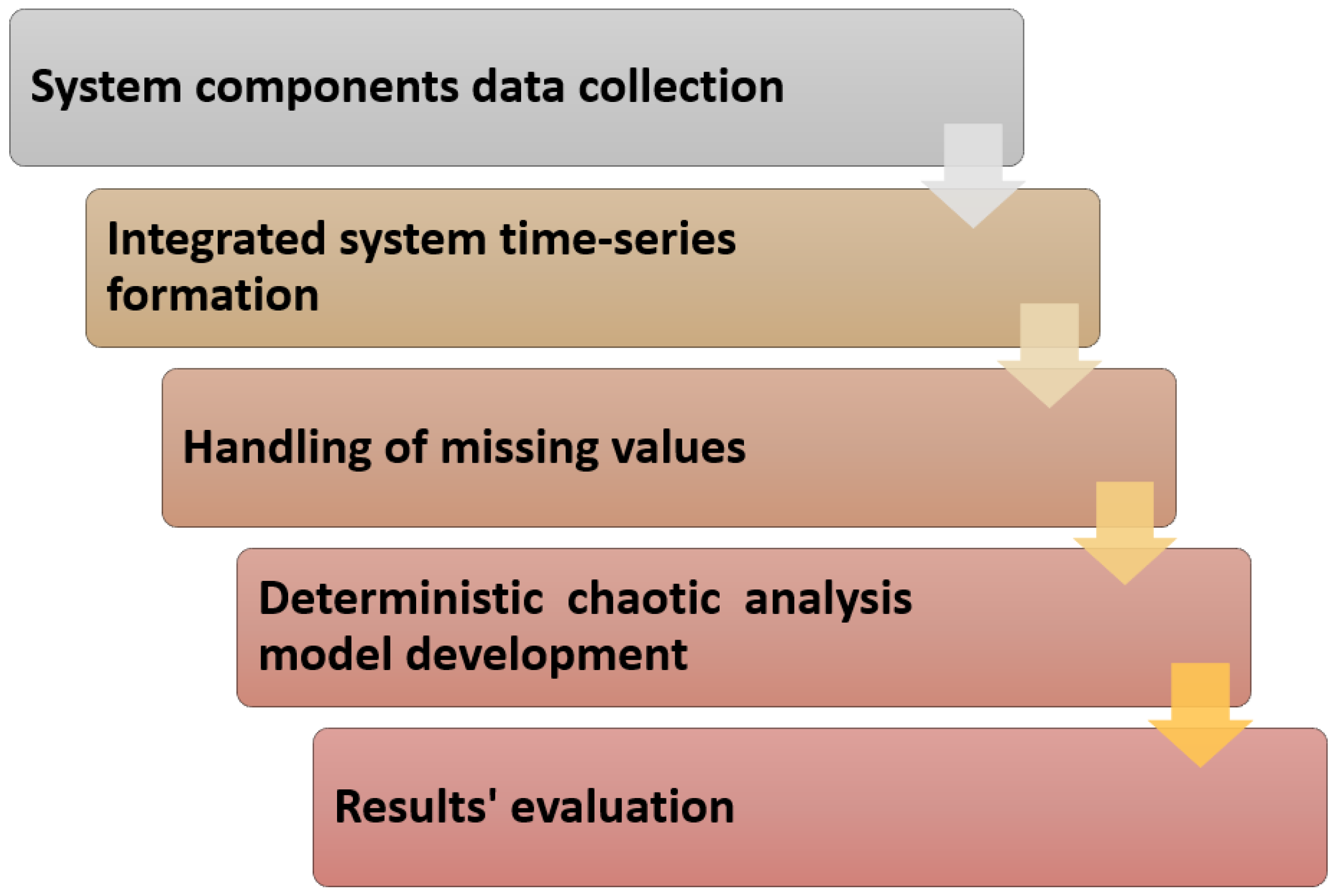
Within the vulnerability analysis and forecasting domain, many research efforts address issues in specific software components, including operating systems, browsers, and application software of different vendors. To the best of our knowledge, there is no research report on vulnerability analysis of software at the integrated (operating system, middleware, application software) system level. Therefore, first the current research effort attempts to fill in this gap. Namely, it attempts, based on a synthesis of specific services deduced from the NVD database, to generate real-life system models by integrating operating system, middleware and application software CVSSs. To this end, we used NVD as the pool from where we extract and process our data.
Secondly, based on the observations of Section 2 it is evident that the modeling or forecasting of results using traditional linear and nonlinear methodologies show promising but relatively poor performance. Knowing that deterministic chaos analysis has offered a successful framework for modeling complex phenomena in many different fields of real-world data, it is worth using such a modeling approach in our case. Therefore, the present case study also aims at determining whether the time series datasets (services in synthesis corresponding to real-life systems) created by the usage of NVD are governed by deterministic chaos. Such a modeling analysis might potentially improve the forecasting of vulnerability and IT security-related time series.

4. Methodology

To develop a deterministic chaotic analysis methodology, we need to identify a series of cyber-security events, their severity in a quantified way, and their inter-dependencies. However, for this methodology to be accurate, we need plenty of data. In this study, as previously mentioned, to create our data set we employed the NVD dataset, which is widely accepted in nearly all research papers on vulnerability analysis [8,29]. We then investigated several deterministic chaotic analysis methods, experimenting with different handling approaches of the data set.
The proposed methodology consists of five steps, as shown in Figure 1. These steps include (1) system components data collection, (2) integrated system time-series formation, (3) handling of missing values, (4) deterministic chaotic analysis model development and (5) evaluation of the results.

4.1. Data Collection

4.1.1. Software System Definition

Initially, we collected all the data from the NIST vulnerability database to mine the available information about the recorded published vulnerabilities of all recorded software. After accumulating the data (as shown in the example in Section 5.1 in more detail), we tried to create logical constructs by integrating the software services comprising synthetic systems to represent the real-life base models as defined in Table 1.
We assume that all the components of each computing system (services) are almost equally critical for its functionality. In this regard, any service failure results in a system failure of the same type, e.g., denial of service, privilege escalation etc. Thus, each system vulnerability score can be defined as the maximum vulnerability CVSS score of each tabled vulnerability component. Based on the NVD accumulated data, we formed representative functioning software systems considering two distinct categories: open source and proprietary source code systems.
Due to the sparseness of the corresponding data sets, we opted to cluster the events in predefined epochs. This approach allows our sample to become dense enough to enable deterministic chaotic analysis methods to function properly. Using configurations of real-world systems, we clustered our data per week or month (depending on the data status on each data set).
In the following, we present an example of the process of data collection from the NVD database to formulate the initial (with missing values) time series dataset. For this purpose, we will use the Openstack controller to illustrate the process. Initially, we create the initial Openstack controller table to house the time series data (the table may contain multiple values in one specific date). The second step is to fill the above table with relevant data, form the main CVSS table (that contains all NVD services data). This is where the synthesis of the services happens and the synthetic base model (abstractions of a real-life system) is created. Then, we create a “final” table that will house the maximum CVSS score related date entries of the above-created table without any redundant values (as explained previously in this section). Finally, we perform the aforementioned “dimensionality reduction” in the values of the initially created table to remove redundant values and keep the ones with the maximum CVSS scores on any given date (as explained previously in this section, the above services might have more than one value in any given date and we must keep the maximum CVSS score value).
As a result, our database consists of the following fields:
  • CVE ID
  • Published datetime
  • Vulnerability Score
  • Vulnerability software list.

4.1.2. NVD Processing

Our focus is to determine whether the time series datasets (extracted as services which are integrated to logically represent base models of real-life systems) created using the NVD database are governed by deterministic chaos. We could use this knowledge to create a more robust forecasting model for our systems while, at the same time, improving relevant forecasting calculations. Several authors approach this by mainly performing the calculations for the largest Lyapunov exponent (LLE), Shannon entropy/Sample entropy (SE) and Hurst exponent (HE) to prove the existence of deterministic chaos in a time series model [58,66,67,68]. As such, we also use the same idea to prove the existence of deterministic chaos in our data set.
To better understand the methodology herein presented, it should be noted that the NVD database contains vulnerability data for specific services. The rows of this database show the vulnerability of a service. To logically construct a computer system representing a real-life system, the relevant services should be synthesized. More specifically, a real-life, for instance Openstack controller server, should run as a minimum the services outlined in Table 1. Therefore, by integrating the relevant rows from the NVD database the system Openstack controller server can be logically created. One understands that such an integration of services constitutes a synthesis representing the base model of the Openstack controller server. The basic assumption of this study is that the risk of the synthesis of services could not be larger than the maximum risk of all independent services. Based on this assumption, we considered the maximum CVSS score in the integration of services. To investigate the chaotic properties of the systems outlined in the above discussion, the present study is split into two distinct efforts:
  • Create 8 synthetic base models (open/closed source) of real-life systems from the services extracted from NVD database and perform the above calculations.
  • Create 1000 synthetic systems as models of open/closed source systems, from randomly selected services extracted from the NVD database and perform the above calculations.
Each system contains several services (as seen in Table 1). For the system to operate, an OS is also needed (that is why we have the distinction between closed source, e.g., Windows server and opensource, e.g., Linux). Based on this, we randomly created 500 closed source and 500 open-source OS-based systems with relevant random services added to them to capture the differences regarding security risks of open and closed source systems. The only difference is that all relevant services are randomly attached to the base OS (closed or open-source OS type) to have an overall random system creation.

4.2. Deterministic Chaos Analysis Methods

As seen in many papers that deal with detecting deterministic chaos in a given dataset [58,66,67,68], one can observe an emerging pattern on how to perform chaotic analysis in datasets in different application domains. The main methods used so far are (but not limited to):
  • The calculation of the Largest Lyapunov exponent (LLE).
  • The calculation of the Hurst exponent (HE) and of the Fractal dimension (FD).
  • The calculation of the Shannon entropy (SE).

4.2.1. Largest Lyapunov Exponent (LLE)

It is known that if the LLE test statistic in a dataset has positive values, this indicates the existence of chaos. A robust and accurate algorithm to calculate LLE is the one developed by Rosenstein [69], which has been proven to be independent, in each calculation result, from the main parameters used: the embedded dimension (emb_dim), the size of the dataset, the noise level and the reconstruction delay (rec_delay). The chaotic dynamics of the data are reconstructed using a reconstruction delay embedding method, in which each data value X i , for the data frame X, is associated with the vector:
X i = [ X i , X i + r e c _ d e l a y , x i + 2 r e c _ d e l a y , , x i + ( e m b _ d i m 1 ) d e l a y ]
where r e c _ d e l a y is the reconstruction delay embedding and e m b _ d i m is the relevant embedding dimension.
For each such vector X i , we seek its closest neighbor X j according to the euclidean distance measure. It is known that in chaotic systems the trajectories of the closest neighbors X i and X j diverge through time in an exponential way. This can be modeled through their euclidean distance d i , j in time noted as d i , j ( t ) . The power law d i , j ( t ) = C e l l e t is used in this modeling, where l l e is the target approximation of the highest Lyapunov exponent in the Rosenstein method.
To calculate l l e , we take the logarithm of the previous power law equation and derive l o g ( d i , j ( t ) ) = l o g ( C ) + ( l l e t ) . This gives a set of lines, for each index pair i , j with a slope equal to the approximation of l l e . If we take the min value of all the l o g ( d i , j ( t ) ) for all vectors X i , then the average line slope over time is the target approximation of l l e .

4.2.2. Fractal Analysis: Hurst Exponent (HE) and Fractal Dimension (FD)

HE is a measure for the “long-term memory” of a time series. HE defines the long statistical dependencies in the data which are not related to cycles. HE originates from the Hursts observations of the problem of long-term storage in water reservoirs [70]. If X i is the discharge of a river in year i and we observe this discharge for N years, we can calculate the storage capacity that would be required to keep the discharge steady at its mean value.
To apply this methodology, we first subtract the mean over all X i ¯ from the individual data points X i in the given time series in order to obtain the residual X i from the mean for each point i. As the excess (or deficit) in this residual is carried from data point i to the next data point i + 1 , the associated cumulative sum of X i , is denoted by Y i . If this cumulative sum is above 0 we have what we call residual excess, otherwise, there is a residual deficit. By considering the range (maximum–minimum) R of Y i , we have an indication of the total variation of the time series with respect to the mean value.
Hurst showed that this value follows a steady trend for varying N, if it is normalized by the standard deviation σ over X i . Namely Hurst obtained the following formula:
R σ = ( N 2 ) K
In this equation, K is called the Hurst exponent. Its value is 0.5 for white noise, but becomes larger for time series that exhibit some positive dependency on previous values, outlining a long term correlation (or long term memory range). For negative dependencies it becomes less than 0.5, outlining an antiperspirant range as it is usually called in the research literature.

4.2.3. Shannon Entropy (SE)

In his seminal work, Shannon introduced the concept of entropy for information theory [71]. The concept is similar to the entropy that is used in thermodynamics, however, the focus on information theory is to gauge the degree of randomness in the values that an information source generates. In this regard, the Shannon entropy (SE) of a time series { X t } t = 1 n is given by:
S E ( x ) = y = 1 n p i l o g ( p i )
where p i is a discrete probability such that i p i = 1 . SE reaches its maximum if all values of the underlying time series { X t } t = 1 n are equally probable. Therefore, the maximum value is l o g n and when SE approaches this value, the time series is nearly random. On the contrary, if there is a single X i for which P ( X i ) = 1 , then, SE reaches its minimum value, which is 0. Practically, the latter denotes that the source generates a single value, hence there is no randomness in the produced sequence.

5. Empirical Analysis and Discussion

To showcase the robustness of our methodology and its efficacy in producing valid modeling results, we perform a step-by-step “construction” of the data as well as perform the necessary non-linear analysis calculations on the first real-world system model “Linux Openstack Control system” presented in Table 1. The results for the rest of the models of the aforementioned table are also reported in the manuscript and discussed in the following sections.

5.1. Systems Time Series Construction and Pre-Processing

The first step in our model development is the construction of the Openstack control system base model. Thus, we extract all the records that contain vulnerabilities that affect the installed software from the NVD data set and record the CVSS score and the corresponding date. More precisely, for the Openstack controller, we consider the following software components: Ubuntu, Linux kernel, IPtables, Fail2ban, RabbitMQ, MySQL, NTP, MongoDB, memcached, apache2, Openstack keystone, Openstack glance, Openstack neutron, Openstack horizon, Openstack nova and Openstack ceilometer. If the dataset contains more than one vulnerability in one day, we keep the maximum score. Obviously, in this case, we could have variations comprised of the minimum, the average, or a weighted sum of the corresponding vulnerability scores. We argue, though, that a security officer would most likely consider the worst-case scenario. Thus, we seek to establish a likelihood pattern for a vulnerability appearance in any given dataset on any given day. The final data set will contain two columns with the dates and the maximum CVSS date scores.
Once we created our the model shown in Table 1, the ratio of the missing values in conjunction with the whole sample set needs to be considered. The values mentioned above, evidently, do not appear daily because the covered timeline is vast, and one does not expect a production system to have vulnerabilities daily. For instance, in this dataset, the first value that was found for the controller node was on “1996/7” and the last on “2020/12”. That is roughly a twenty-four-year time-frame, which makes it possible that many values are missing. Figure 2 illustrates the sparsity of the dataset for the OpenStack controller node and depicts the CVSS score of each vulnerability.
The sample is sparse in the beginning, and it started to become denser in recent years. This means that to use some of the standard forecasting methods, we need to address the missing values. We used the K-Nearest Neighbors (KNN) algorithm to handle our missing data. KNN, which belongs to the imputation family of methods, was introduced in [72] and later refined in [73] as a classification method. This method was later refined further and added to the scikit-learn python library to deal with missing values. The KNN algorithm is applied to the dataset, and the obtained values are used to substitute the missing ones.
KNN has proved to be a robust method even when a high proportion of data is missing [74]. Once the KNN imputation model is generated, the next step is to shift through the time series values involving a Fast Fourier Transform (FFT)-based signal reconstruction procedure to validate that the sampling frequency does not violate the Nyquist criterion. This shifting procedure decreases the time windows, starting from the initial NVD dates and ending at the first date X that the time series window [ X d a t e , c u r r e n t d a t e ] can be reconstructed in terms of frequencies.
Based on the above-described procedure, we found empirically that in our data, the “30% missing values” barrier should not be exceeded for a reliable time series reconstruction. In general, when missing values are above a specific threshold in a sample that is not big, the ability of a missing-value-handling algorithm to perform satisfactorily its intended function is hindered. Therefore, “30%” is a relatively acceptable value used to indicate an upper threshold. We have detected that the various missing values algorithms do not guarantee consistent data recovery from that point on. From our experience, 25% to 30% can be a fairly good threshold, and, as such, all temporal data consolidations that exhibit higher missing values are dropped from being analysed. Practically, this means that the missing values must not exceed the 30% missing value barrier if we want our imputation method (KNN in this case) to be accurate. These considerations and remarks comply fully with the outcomes of a recent analysis of the KNN robustness in several data sets with regards to missing value imputation performance [74]. To overcome this issue, we opted to use a week-long interval for the internal data grouping window. We take the week as our minimal temporal unit, which is used in the missing value algorithm. If a sufficient window for non-linear analysis cannot be created (using the week-long data), then a month-long data interval could be formed for further processing.
Therefore, to handle the missing data, we first grouped the data in week intervals. While there are weeks with no vulnerabilities, some of them have more than one. Therefore, we have three approaches:
  • In the Extreme approach, we use the maximum value of each day/week/month interval to fill the weekly score column.
  • In the Average approach, we use the average of each day/week/month values to fill the weekly score column.
  • Finally, in the Relaxed approach, we use the minimum value in each day/week/month interval to fill the weekly score column.
For each approach, we used the KNN algorithm to fill the missing values.

5.2. Application of Non Linear Deterministic Chaotic Analysis Methods to the Defined Systems Time Series

After the formation of the systems time series, the application of the above defined methodologies for deterministic chaotic analysis follows (LLE, HE and SE).

5.2.1. LLE Estimation

A system containing a positive LLE is defined to be chaotic. The magnitude of the exponent reflects the time scale on which the system’s dynamics become unpredictable. In this study, the estimation of the largest Lyapunov exponent is conducted through the Rosenstein algorithm using the python Nolds library [75]. Even though the library provides default values for the dimensions required by the algorithm to work, it is highly encouraged to experiment with these dimensions to find the tested system’s boundaries. The Python function representing the algorithm with the respected default values is:
n o l d s . l y a p _ r ( d a t a , e m b _ d i m = 10 , l a g = N o n e , m i n _ t s e p = N o n e , t a u = 1 , m i n _ n e i g h b o r s = 20 , t r a j e c t o r y _ l e n = 20 , f i t = u R A N S A C , d e b u g _ p l o t = F a l s e , d e b u g _ d a t a = F a l s e , p l o t _ f i l e = N o n e , f i t _ o f f s e t = 0 )
From the above parameters we experimented with t r a j e c t o r y _ l e n , e m b _ d i m , m i n _ n e i g h b o r s , and l a g , and for the rest we used the default values.

5.2.2. HE Estimation

With regards to the Hurst exponent, we also use the Nolds Python library to calculate it. The Hurst exponent varies between 0 and 1, and the interpretation of the coefficient is as follows: for 0.5 < H < 1 , the process has a long stationary memory; for H = 0.5 , the time series obeys random walk; in the case where 0 < H < 0.5 , the series is said to be antipersistent. The Python function representing the algorithm with the respected dimensions is:
n o l d s . h u r s t _ r s ( d a t a , n v a l s = N o n e , f i t = u R A N S A C , d e b u g _ p l o t = F a l s e , d e b u g _ d a t a = F a l s e , p l o t _ f i l e = N o n e , c o r r e c t e d = T r u e , u n b i a s e d = T r u e )
We use the default values for the required dimensions as presented from above.

5.2.3. SE Estimation

The Shannon entropy Equation (see Section 4.2.3) has been implemented using NumPy and SciPy Python libraries and it has been applied to all defined time series. There are no user parameters required for calculating SE.

5.3. Computational Overhead

It should be noted that, the setup of the computing system used to perform the experiments was a i7-6700 CPU (3.4 GHz) with 8 cores, 32 GB DDR4 RAM and 1TB SSD hard disk drive.
The processing time needed for computing LLE (for each possible combination of t r a j e c t o r y _ l e n , e m b _ d i m , m i n _ n e i g h b o r s and l a g ), HE, and SE was 26 s, 0.336 s, and 0.018 s, respectively for the eight base systems presented in Table 1 and was 1378.75 s, 7.36 s, and 0.073 s, respectively for the random generated systems.
Please note that in the first case, we did not use any parallelisation for our computations. Therefore, further performance improvements can be achieved in a production environment. In the second case, we used parallelisation for our computations via the Python Joblib library only for the LLE and HE calculations.

6. Discussion of the Results

In what follows, we interpret the measurements of our dataset from the previous section. The goal is to determine whether the measurements exhibit the properties that one would find in a chaotic system.
Regarding the LLE analysis, by reviewing the results presented in Table 2, Table 3, Table 4, Table 5, Table 6, Table 7, Table 8 and Table 9 we can see that for the randomly generated systems in both cases (500 closed source/500 open source), we have a positive value for more than 60% of the total values calculated. Furthermore, we analyze the results based on different combinations of the parameters used by the Nolds Python library to calculate LLE. We can see that for specific value combinations (total 24/26 rows for closed/open source, Table 6, Table 7, Table 8 and Table 9), all random systems have positive LLEs. Therefore, these combinations lead to strong evidence of the existence of a chaotic behavior in our systems. The above-mentioned Nold’s Python library parameter sequences used in the implementation of Rosenstein method are:
  • t r a j e c t o r y _ l e n : 6, 7 and 8.
  • e m b _ d i m : 5 and 7.
  • m i n _ n e i g h b o r s : 3, 4 and 5.
  • l a g : 1 and 2.
Please note that the necessary and sufficient condition to prove the existence of deterministic chaos in a time series is to find proper values of the parameters of the Rosenstein method to satisfy L L E > 0 . The fact that we have several parameter values leading to positive LLEs shows several ways to define the time series chaotic space. Finding the exact embedding dimension and lag is subject to future research.
Similar results hold for the eight synthetic base models of real-life systems. In these systems 69% of the cases in total for all parameters variations tested (with the testing plan mentioned above) have positive Lyapunov exponents. Moreover, it is worth noting that a larger percentage of open source systems ( 72 % ) are chaotic compared to closed source systems ( 62 % ) (see Table 5). Such a result might mean that closed-form systems are more systematically subject to attacks than open source systems.
Regarding HE, by reviewing the results presented in Table 10 and Table 11 and by grouping the values into bins based on the interpretation mentioned above, we can see that in the majority of the 1000 randomly generated systems these values are in the [0.40–0.49] and [0.51–0.60] zones, which are characterized as peak chaotic zones. This is of particular interest, because, based on the analysis in [76], these ranges are also found to apply for the chaotic zone during the investigation of whether a correlation between HEs and LLEs exists. Using the methodology presented in [76] the following is observed: A map function (well known for displaying deterministic chaos) is used as the basis to perform this investigation and the results show that while regular noise corresponds to H ≈ 0, the peak of this map function is related to the chaotic zone at H = 0.40 0.60 and with a steady gradient in between. Performing a similar experiment using the vulnerability data herein presented, it is obtained that (based also on the LLEs parameters found) a correlation exists between the peak chaotic zone and the bulk of the Hurst exponents values and, also this correlation is found on the same corresponding zones as in [76].
By further analysing the results of Table 10, we notice that the closed systems related to HE are in the range [0.40–0.49], which corresponds to the antipersistent range, whereas the open source systems related HE is in the range [0.51–0.60], which corresponds to the long term memory range. Both closed and open source systems present around only 10 % of the cases in the random walk range [0.50–0.51]. Based also on the results presented in Table 11, we notice that regarding the closed source servers, the Microsoft Dot Net Application and the Microsoft Database Server, fall into the antipersistent range in the boundaries of the ranges defined in [76]. On the other hand, the Microsoft Mail Server corresponds to the antipersistent range in accordance with the range defined in [76].
Considering the open-source systems, all relevant HE fall into the stationary long term memory in agreement with the range defined in [76] except for the Linux Database Server HE, which corresponds to the antipersistent range defined in [76]. Moreover, based on Table 10, it seems that more open source systems ( 77 % ) are in the chaotic region associated with HE compared to closed source systems ( 65 % ) .
Regarding SE, the results of Table 11, Table 12 and Table 13 clearly show that the number of bits (entropy) and also the average number of bits (mean entropy) calculated by SE are much larger than zero and much smaller than the number of bits of the end systems samples ( l o g s 2 N ). If the number of bits calculated by SE is larger than zero, then the corresponding system is characterized by uncertainty. On the other hand, if the number of bits is near the maximum number of bits, which is the number of bits of the system samples ( l o g s 2 N ), then the corresponding system is characterised by complete randomness. Therefore, it is obvious that based on Table 11, regarding the base model systems (Table 1), the associated time series are characterised by chaotic dynamics and uncertainty. The same conclusion is derived for both closed and open source random generated systems. However, it should be noticed that open source systems present a larger uncertainty than closed source systems.
Based on the above analysis and the individual measurements of LLE, HE, and SE, the generated systems do not have random vulnerabilities. Quite the contrary, they follow the properties of a chaotic system. Moreover, since this observation is derived from three independent measures, it is more than evident that any underlying system is a chaotic system. The results are important since they reveal a hidden pattern in system-wide vulnerabilities of IS. More importantly, the above findings justify the failure of the existing methods’ in accurately predicting vulnerabilities in the long term. Further to merely providing this justification, the chaotic nature implies that chaos-based methodologies can provide more accurate predictions and pave the way for new security-oriented applications.

Limitations

Undoubtedly, the literature presents (apart from the LLE, HE, and SE measures investigated above) many other relevant chaotic analysis measures that could be used; however, they are not so widely applied. Therefore, although this study could be significantly extended with the application of other non-linear analysis metrics, the conclusions derived in the present experimental study are statistically significant due to the large scale experimental data involved. In future work, we plan to include such measures as well.
Another limitation of this work is the usage of a synthesised dataset and not of real-world data collected from the computed systems of an actual enterprise. To the best of our knowledge, there is no such public dataset available. Nevertheless, even in this case, we notice the persistence of patterns that clearly indicate the dataset’s chaotic nature and their deviation from the randomness.

7. Conclusions and Future Prospects

This paper presented a statistically significant non-linear deterministic chaotic analysis framework for computer systems vulnerability time-series. More specifically, the definition of computer systems vulnerabilities was introduced in NIST vulnerability database. The provided definition of open source and close source systems was employed to investigate specific properties in terms of vulnerability characteristics for such systems. Three specific measures of chaotic properties were used. In particular, LLE, HE and SE were selected due to their widespread use in the literature. Based on the experimental study presented, both closed and open source systems vulnerability time series clearly demonstrate chaotic properties. More specifically, the vast majority of such systems’ times series result in positive LLEs, HEs in the chaotic regions and SEs in the region of uncertainty.
The results of this research effort are not only significant in characterising the available vulnerability time series. They are also important for future studies, especially for providing the means for improving vulnerability time series forecasting. Moreover, the contribution of this study implies that the associated time series are not fully predictable. However, the strong evidence of their illustrated chaotic properties could lead to a deeper analysis of the associated systems to improve risk management assessment. The probabilistic analysis of these results indicates that the prediction of vulnerability scores using time series of vulnerability data is a promising approach with far-reaching implications for adopting proper security management measures. Therefore, an important future research goal is to design a risk management framework based on the analysis presented in this paper. Such a framework is still missing from the academic literature and could be applied in the IS security domain of medium and large scale enterprises.

Author Contributions

Conceptualization, C.P.; methodology, C.D. and T.K.D.; software, I.T.; validation, I.T. and T.K.D.; formal analysis, T.K.D. and C.P.; investigation, I.T., T.K.D. and C.P.; data curation, I.T.; writing—original draft preparation, I.T., T.K.D., C.D. and C.P.; writing—review and editing, I.T., T.K.D., C.D. and C.P.; visualization, I.T.; supervision, C.D. and C.P.; project administration, C.P.; funding acquisition, C.D. and C.P. All authors have read and agreed to the published version of the manuscript.

Funding

This work was supported by the European Commission under the Horizon 2020 Programme (H2020), as part of the project CyberSec4Europe (https://www.cybersec4europe.eu) (Grant Agreement no. 830929). This work has also been co-financed by the IntelTriage ("Intelligent triage system for hospital emergency departments and clinics") and MELITY ("Development of methodologies and embedded security solutions for e-health services based on Internet of Things technologies") projects which are financially supported by the European Union and the Greek national funds through the operation program Competitiveness, Entrepreneurship and Innovation under the call RESEARCH-CREATE-INNOVATE (T1EDK-02489 and T1EDK-01958).

Institutional Review Board Statement

Not applicable.

Informed Consent Statement

Not applicable.

Data Availability Statement

Not applicable.

Acknowledgments

The content of this article does not reflect the official opinion of the European Union. Responsibility for the information and views expressed therein lies entirely with the authors.

Conflicts of Interest

The authors declare no conflict of interest.

References

  1. Schultz, E.E., Jr.; Brown, D.S.; Longstaff, T.A. Responding to Computer Security Incidents: Guidelines for Incident Handling; Technical Report; No. UCRL-ID-104689; Lawrence Livermore National Lab: Livermore, CA, USA, 1990. [Google Scholar]
  2. Alhazmi, O.H.; Malaiya, Y.K.; Ray, I. Measuring, analyzing and predicting security vulnerabilities in software systems. Comput. Secur. 2007, 26, 219–228. [Google Scholar] [CrossRef]
  3. Hassan, S.G.; Iqbal, S.; Garg, H.; Hassan, M.; Shuangyin, L.; Kieuvan, T.T. Designing Intuitionistic Fuzzy Forecasting Model Combined With Information Granules and Weighted Association Reasoning. IEEE Access 2020, 8, 141090–141103. [Google Scholar] [CrossRef]
  4. Kakimoto, M.; Endoh, Y.; Shin, H.; Ikeda, R.; Kusaka, H. Probabilistic solar irradiance forecasting by conditioning joint probability method and its application to electric power trading. IEEE Trans. Sustain. Energy 2018, 10, 983–993. [Google Scholar] [CrossRef]
  5. Alhazmi, O.H.; Malaiya, Y.K. Application of vulnerability discovery models to major operating systems. IEEE Trans. Reliab. 2008, 57, 14–22. [Google Scholar] [CrossRef]
  6. Alhazmi, O.H.; Malaiya, Y.K. Prediction capabilities of vulnerability discovery models. In Proceedings of the Reliability and Maintainability Symposium, RAMS’06, Newport Beach, CA, USA, 23–26 January 2006; pp. 86–91. [Google Scholar]
  7. Roumani, Y.; Nwankpa, J.K.; Roumani, Y.F. Time series modeling of vulnerabilities. Comput. Secur. 2015, 51, 32–40. [Google Scholar] [CrossRef]
  8. Johnson, P.; Gorton, D.; Lagerström, R.; Ekstedt, M. Time between vulnerability disclosures: A measure of software product vulnerability. Comput. Secur. 2016, 62, 278–295. [Google Scholar] [CrossRef]
  9. Zhang, S.; Caragea, D.; Ou, X. An empirical study on using the national vulnerability database to predict software vulnerabilities. In International Conference on Database and Expert Systems Applications; Springer: Berlin/Heidelberg, Germany, 2011; pp. 217–231. [Google Scholar]
  10. Nguyen, V.H.; Massacci, F. A Systematically Empirical Evaluation Of Vulnerability Discovery Models: A Study On Browsers’ Vulnerabilities. arXiv 2013, arXiv:1306.2476. [Google Scholar]
  11. Tang, M.; Alazab, M.; Luo, Y.; Donlon, M. Disclosure of cyber security vulnerabilities: Time series modelling. Int. J. Electron. Secur. Digit. Forensics 2018, 10, 255–275. [Google Scholar] [CrossRef]
  12. Shrivastava, A.K.; Sharma, R. Modeling Vulnerability Discovery and Patching with Fixing Lag; Springer: Berlin/Heidelberg, Germany, 2019. [Google Scholar]
  13. Williams, M.A.; Dey, S.; Barranco, R.C.; Naim, S.M.; Hossain, M.S.; Akbar, M. Analyzing Evolving Trends of Vulnerabilities in National Vulnerability Database. In Proceedings of the 2018 IEEE International Conference on Big Data (Big Data), Seattle, WA, USA, 10–13 December 2018; pp. 3011–3020. [Google Scholar]
  14. Sharma, R.; Singh, R.K. Vulnerability Discovery in Open- and Closed-Source Software: A New Paradigm. In Software Engineering; Springer: Singapore, 2019; pp. 533–539. [Google Scholar]
  15. Johnston, R.; Sarkani, S.; Mazzuchi, T.; Holzer, T.; Eveleigh, T. Bayesian-model averaging using MCMCBayes for web-browser vulnerability discovery. Reliab. Eng. Syst. Saf. 2019, 183, 341–359. [Google Scholar] [CrossRef]
  16. Johnson, P.; Lagerstrom, R.; Ekstedt, M.; Franke, U. Can the common vulnerability scoring system be trusted? A Bayesian analysis. IEEE Trans. Dependable Secur. Comput. 2018, 15, 1002–1015. [Google Scholar] [CrossRef]
  17. Biswas, B.; Mukhopadhyay, A. G-RAM framework for software risk assessment and mitigation strategies in organisations. J. Enterp. Inf. Manag. 2018, 31, 276–299. [Google Scholar] [CrossRef]
  18. Jimenez, M.; Papadakis, M.; Traon, Y.L. Vulnerability Prediction Models: A Case Study on the Linux Kernel. In Proceedings of the 2016 IEEE 16th International Working Conference on Source Code Analysis and Manipulation, Raleigh, NC, USA, 2–3 October 2016; pp. 1–10. [Google Scholar]
  19. Sahin, S.E.; Tosun, A. A Conceptual Replication on Predicting the Severity of Software Vulnerabilities. In Proceedings of the Evaluation and Assessment on Software Engineering, Copenhagen, Denmark, 15–17 April 2019; pp. 244–250. [Google Scholar]
  20. Spanos, G.; Angelis, L. A multi-target approach to estimate software vulnerability characteristics and severity scores. J. Syst. Softw. 2018, 146, 152–166. [Google Scholar] [CrossRef]
  21. Zhu, X.; Cao, C.; Zhang, J. Vulnerability severity prediction and risk metric modeling for software. Appl. Intell. 2017, 47, 828–836. [Google Scholar] [CrossRef]
  22. Geng, J.; Ye, D.; Luo, P. Predicting Severity of Software Vulnerability Based on Grey System Theory. In International Conference on Algorithms and Architectures for Parallel Processing; Springer: Berlin/Heidelberg, Germany, 2015. [Google Scholar]
  23. Geng, J.; Ye, D.; Luo, P. Forecasting Severity of Software Vulnerability Using Grey Model GM(1,1). In Proceedings of the 2015 IEEE Advanced Information Technology, Electronic and Automation Control Conference (IAEAC), Chongqing, China, 19–20 December 2015; pp. 344–348. [Google Scholar]
  24. Ozment, A. Improving Vulnerability Discovery Models: Problems with Definitions and Assumptions. In Proceedings of the 2007 ACM Workshop on Quality of Protection, Lexandria, VA, USA, 29 October 2007; pp. 6–11. [Google Scholar]
  25. Shamal, P.K.; Rahamathulla, K.; Akbar, A. A Study on Software Vulnerability Prediction Model. In Proceedings of the 2017 International Conference on Wireless Communications, Signal Processing and Networking (WiSPNET), Chennai, India, 22–24 April 2017; pp. 703–706. [Google Scholar]
  26. Wu, W.; Zhang, W.; Yang, Y.; Wang, Q. Time series analysis for bug number prediction. In Proceedings of the 2nd International Conference on Software Engineering and Data Mining, Chengdu, China, 23–25 June 2010; pp. 589–596. [Google Scholar]
  27. Morrison, P.; Herzig, K.; Murphy, B.; Williams, L. Challenges with Applying Vulnerability Prediction Models. In Proceedings of the 2015 Symposium and Bootcamp on the Science of Security, Urbana, IL, USA, 21–22 April 2015; pp. 1–9. [Google Scholar]
  28. Gencer, K.; Başçiftçi, F. Time series forecast modeling of vulnerabilities in the android operating system using ARIMA and deep learning methods. Sustain. Comput. Inform. Syst. 2021, 30. [Google Scholar] [CrossRef]
  29. Last, D. Using historical software vulnerability data to forecast future vulnerabilities. In Proceedings of the Resilience Week (RWS), Philadelphia, PA, USA, 18–20 August 2015; pp. 1–7. [Google Scholar]
  30. Shrivastava, A.K.; Sharma, R.; Kapur, P.K. Vulnerability Discovery Model for a Software System Using Stochastic Differential Equation. In Proceedings of the 2015 International Conference on Futuristic Trends on Computational Analysis and Knowledge Management (ABLAZE), Greater Noida, India, 26–27 February 2015; pp. 199–205. [Google Scholar]
  31. Tang, M.; Alazab, M.; Luo, Y. Exploiting Vulnerability Disclosures: Statistical Framework and Case Study. In Proceedings of the Cybersecurity and Cyberforensics Conference (CCC), Amman, Jordan, 2–4 August 2016; pp. 117–122. [Google Scholar]
  32. Chatzipoulidis, A.; Michalopoulos, D.; Mavridis, I. Information infrastructure risk prediction through platform vulnerability analysis. J. Syst. Softw. 2015, 106, 28–41. [Google Scholar] [CrossRef]
  33. Woo, S.W.; Joh, H.; Alhazmi, O.H.; Malaiya, Y.K. Modeling vulnerability discovery process in Apache and IIS HTTP servers. Comput. Secur. 2011, 30, 50–62. [Google Scholar] [CrossRef]
  34. Wang, X.; Ma, R.; Li, B.; Tian, D.; Wang, X. E-WBM: An Effort-Based Vulnerability Discovery Model. IEEE Access 2019, 7, 44276–44292. [Google Scholar] [CrossRef]
  35. Kudjo, P.K.; Chen, J.; Mensah, S.; Amankwah, R. Predicting Vulnerable Software Components via Bellwethers. In Chinese Conference on Trusted Computing and Information Security; Springer: Singapore, 2018; pp. 389–407. [Google Scholar]
  36. Li, Z.; Shao, Y. A Survey of Feature Selection for Vulnerability Prediction Using Feature-Based Machine Learning. In Proceedings of the 2019 11th International Conference on Machine Learning and Computing, Zhuhai, China, 22–24 February 2019; Volume Part F1481, pp. 36–42. [Google Scholar]
  37. Wei, S.; Zhong, H.; Shan, C.; Ye, L.; Du, X.; Guizani, M. Vulnerability Prediction Based on Weighted Software Network for Secure Software Building. In Proceedings of the 2018 IEEE Global Communications Conference (GLOBECOM), Abu Dhabi, United Arab Emirates, 9–13 December 2018. [Google Scholar]
  38. Nguyen, T.K.; Ly, V.D.; Hwang, S.O. An efficient neural network model for time series forecasting of malware. J. Intell. Fuzzy Syst. 2018, 35, 6089–6100. [Google Scholar] [CrossRef]
  39. Catal, C.; Akbulut, A.; Ekenoglu, E.; Alemdaroglu, M. Development of a Software Vulnerability Prediction Web Service Based on Artificial Neural Networks; Springer: Berlin/Heidelberg, Germany, 2017. [Google Scholar]
  40. Alves, H.; Fonseca, B.; Antunes, N. Experimenting Machine Learning Techniques to Predict Vulnerabilities. In Proceedings of the 2016 Seventh Latin-American Symposium on Dependable Computing (LADC), Cali, Colombia, 19–21 October 2016; pp. 151–156. [Google Scholar]
  41. Last, D. Forecasting Zero-Day Vulnerabilities. In Proceedings of the 11th Annual Cyber and Information Security Research Conference, Oak Ridge, TN, USA, 5–7 April 2016; p. 13. [Google Scholar]
  42. Pang, Y.; Xue, X.; Wang, H. Predicting Vulnerable Software Components through Deep Neural Network. In Proceedings of the 2017 International Conference on Deep Learning Technologies, Chengdu, China, 2–4 June 2017; Volume Part F1285, pp. 6–10. [Google Scholar]
  43. Walden, J.; Stuckman, J.; Scandariato, R. Predicting Vulnerable Components: Software Metrics vs. Text Mining. In Proceedings of the 2014 IEEE 25th International Symposium on Software Reliability Engineering, Naples, Italy, 3–6 November 2014; pp. 23–33. [Google Scholar]
  44. Scandariato, R.; Walden, J.; Hovsepyan, A.; Joosen, W. Predicting vulnerable software components via text mining. IEEE Trans. Softw. Eng. 2014, 40, 993–1006. [Google Scholar] [CrossRef]
  45. Wei, S.; Du, X.; Hu, C.; Shan, C. Predicting Vulnerable Software Components Using Software Network Graph; Springer: Berlin/Heidelberg, Germany, 2017. [Google Scholar]
  46. Kansal, Y.; Kapur, P.K.; Kumar, U.; Kumar, D. Prioritising vulnerabilities using ANP and evaluating their optimal discovery and patch release time. Int. J. Math. Oper. Res. 2019, 14, 236–267. [Google Scholar] [CrossRef]
  47. Zhang, M.; De Carne De Carnavalet, X.; Wang, L.; Ragab, A. Large-scale empirical study of important features indicative of discovered vulnerabilities to assess application security. IEEE Trans. Inf. Forensics Secur. 2019, 14, 2315–2330. [Google Scholar] [CrossRef]
  48. Jimenez, M.; Papadakis, M.; Traon, Y.L. An Empirical Analysis of Vulnerabilities in OpenSSL and the Linux Kernel. In Proceedings of the 2016 23rd Asia-Pacific Software Engineering Conference (APSEC), Hamilton, New Zealand, 6–9 December 2016; pp. 105–112. [Google Scholar]
  49. Siavvas, M.; Kehagias, D.; Tzovaras, D. A Preliminary Study on the Relationship among Software Metrics and Specific Vulnerability Types. In Proceedings of the 2017 International Conference on Computational Science and Computational Intelligence (CSCI), Las Vegas, NV, USA, 14–16 December 2017; pp. 916–921. [Google Scholar]
  50. Wai, F.K.; Yong, L.W.; Divakaran, D.M.; Thing, V.L.L. Predicting Vulnerability Discovery Rate Using Past Versions of a Software. In Proceedings of the 2018 IEEE International Conference on Service Operations and Logistics, and Informatics (SOLI), Singapore, 31 July–2 August 2018; pp. 220–225. [Google Scholar]
  51. Rahimi, S.; Zargham, M. Vulnerability scrying method for software vulnerability discovery prediction without a vulnerability database. IEEE Trans. Reliab. 2013, 62, 395–407. [Google Scholar] [CrossRef]
  52. Munaiah, N. Assisted Discovery of Software Vulnerabilities. In Proceedings of the 40th International Conference on Software Engineering: Companion Proceeedings, New York, NY, USA, 30 May–1 June 2018; pp. 464–467. [Google Scholar]
  53. Javed, Y.; Alenezi, M.; Akour, M.; Alzyod, A. Discovering the relationship between software complexity and software vulnerabilities. J. Theor. Appl. Inf. Technol. 2018, 96, 4690–4699. [Google Scholar]
  54. Last, D. Consensus Forecasting of Zero-Day Vulnerabilities for Network Security. In Proceedings of the 2016 IEEE International Carnahan Conference on Security Technology (ICCST), Orlando, FL, USA, 24–27 October 2016. [Google Scholar]
  55. Han, Z.; Li, X.; Xing, Z.; Liu, H.; Feng, Z. Learning to Predict Severity of Software Vulnerability Using Only Vulnerability Description. In Proceedings of the 2017 IEEE International Conference on Software Maintenance and Evolution (ICSME), Shanghai, China, 17–22 September 2017; pp. 125–136. [Google Scholar]
  56. Heltberg, M.L.; Krishna, S.; Kadanoff, L.P.; Jensen, M.H. A tale of two rhythms: Locked clocks and chaos in biology. Cell Syst. 2021, 12, 291–303. [Google Scholar] [CrossRef]
  57. Jiang, K.; Qiao, J.; Lan, Y. Chaotic renormalization flow in the Potts model induced by long-range competition. Phys. Rev. E 2021, 103. [Google Scholar] [CrossRef] [PubMed]
  58. Lahmiri, S.; Bekiros, S. Cryptocurrency forecasting with deep learning chaotic neural networks. Chaos Solitons Fractals 2019, 118, 35–40. [Google Scholar] [CrossRef]
  59. Yan, B.; Chan, P.W.; Li, Q.; He, Y.; Shu, Z. Dynamic analysis of meteorological time series in Hong Kong: A nonlinear perspective. Int. J. Climatol. 2021, 41, 4920–4932. [Google Scholar] [CrossRef]
  60. Picano, B.; Chiti, F.; Fantacci, R.; Han, Z. Passengers Demand Forecasting Based on Chaos Theory. In Proceedings of the ICC 2019—2019 IEEE International Conference on Communications (ICC), Shanghai, China, 20–24 May 2019; pp. 1–6. [Google Scholar]
  61. Kawauchi, S.; Sugihara, H.; Sasaki, H. Development of very-short-term load forecasting based on chaos theory. Electr. Eng. Jpn. 2004, 148, 55–63. [Google Scholar] [CrossRef]
  62. Liu, X.; Fang, X.; Qin, Z.; Ye, C.; Xie, M. A Short-term forecasting algorithm for network traffic based on chaos theory and SVM. J. Netw. Syst. Manag. 2011, 19, 427–447. [Google Scholar] [CrossRef]
  63. Fouladi, R.F.; Ermiş, O.; Anarim, E. A DDoS attack detection and defense scheme using time-series analysis for SDN. J. Inf. Secur. Appl. 2020, 54. [Google Scholar] [CrossRef]
  64. Procopiou, A.; Komninos, N.; Douligeris, C. ForChaos: Real Time Application DDoS Detection Using Forecasting and Chaos Theory in Smart Home IoT Network. Wirel. Commun. Mob. Comput. 2019, 2019, 8469410. [Google Scholar] [CrossRef]
  65. Devaney, R.L. An Introduction to Chaotic Dynamical Systems; Chapman and Hall/CRC: Boca Raton, FL, USA, 1989. [Google Scholar]
  66. Lahmiri, S.; Bekiros, S. Chaos, randomness and multi-fractality in Bitcoin market. Chaos Solitons Fractals 2018, 106, 28–34. [Google Scholar] [CrossRef]
  67. Gunay, S.; Kaşkaloğlu, K. Seeking a Chaotic Order in the Cryptocurrency Market. Math. Comput. Appl. 2019, 24, 36. [Google Scholar] [CrossRef] [Green Version]
  68. da Silva Filho, A.C.; Maganini, N.D.; de Almeida, E.F. Multifractal analysis of Bitcoin market. Phys. A Stat. Mech. Its Appl. 2018, 512, 954–967. [Google Scholar] [CrossRef]
  69. Rosenstein, M.T.; Collins, J.J.; De Luca, C.J. A practical method for calculating largest Lyapunov exponents from small data sets. Phys. D Nonlinear Phenom. 1993, 65, 117–134. [Google Scholar] [CrossRef]
  70. Hurst, H.E. The problem of long-term storage in reservoirs. Hydrol. Sci. J. 1956, 1, 13–27. [Google Scholar] [CrossRef] [Green Version]
  71. Shannon, C.E. A mathematical theory of communication. Bell Syst. Tech. J. 1948, 27, 379–423. [Google Scholar] [CrossRef] [Green Version]
  72. Fix, E.; Hodges, J.L. Discriminatory analysis. Nonparametric discrimination: Consistency properties. Int. Stat. Rev. Int. De Stat. 1989, 57, 238–247. [Google Scholar] [CrossRef]
  73. Altman, N.S. An introduction to kernel and nearest-neighbor nonparametric regression. Am. Stat. 1992, 46, 175–185. [Google Scholar]
  74. Batista, G.E.; Monard, M.C. A study of K-nearest neighbour as an imputation method. His 2002, 87, 48. [Google Scholar]
  75. Schölzel, C. NOnLinear Measures for Dynamical Systems (Nolds). Available online: https://github.com/CSchoel/nolds (accessed on 6 September 2021).
  76. Tarnopolski, M. Correlation between the Hurst exponent and the maximal Lyapunov exponent: Examining some low-dimensional conservative maps. Phys. A Stat. Mech. Its Appl. 2018, 490, 834–844. [Google Scholar] [CrossRef] [Green Version]
Figure 1. Methodology.
Informatics 08 00086 g001
Figure 2. Openstack controller vulnerability scores over time.
Informatics 08 00086 g002
Table 1. Model systems definition used for vulnerability analysis.
General Server TypeUsed Services
Open Source CodeLinux Openstack Control ServerUbuntu, Linux kernel, IPtables, Fail2ban, RabbitMQ, MySQL, NTP, MongoDB, memcached, apache2, Openstack keystone, Openstack glance, Openstack neutron, Openstack horizon, Openstack nova, Openstack ceilometer
Linux Openstack Compute ServerUbuntu, Linux kernel, IPtables, Fail2ban, NTP, Openstack neutron, Openstack nova, Openstack ceilometer
Linux Mail ServerUbuntu, Linux kernel, IPtables, Fail2ban, Zimbra, clamAV, SpamAssassin, ufw, Ltab
Linux Java Application ServerUbuntu, Linux kernel, IPtables, Fail2ban, clamAV, ufw, Ltab, JBoss (or TomCat), Java
Linux Database ServerUbuntu, Linux kernel, IPtables, Fail2ban, clamAV, ufw, Ltab, MySQL (or PostgreSQL)
Proprietary Source CodeMicrosoft Mail ServerMicrosoft Windows Server, Microsoft Exchange, Spam Assassin, McAfee, Active Directory
Microsoft Dot Net Application ServerMicrosoft Windows Server, Dot Net Framework, McAfee, Active Directory, IIS
Microsoft Database ServerMicrosoft Windows Server, Microsoft SQL Server, McAfee, Active Directory
Table 2. Largest Lyapunov Exponents for trajectory_len = 6 regarding base model systems.
emb_dim3
min_neighbors2345
lag1234123412341234
>07744774477448744
<01144114411440144
emb_dim5
min_neighbors2345
lag1234123412341234
>08873886388738863
<00015002500150025
emb_dim7
min_neighbors2345
lag1234123412341234
>08845884588448845
<00043004300440043
Table 3. Largest Lyapunov Exponents for trajectory_len = 7 regarding base model systems.
emb_dim3
min_neighbors2345
lag1234123412341234
>02536253525362535
<06352635363526353
emb_dim5
min_neighbors2345
lag1234123412341234
>08663886487638764
<00225002401250124
emb_dim7
min_neighbors2345
lag1234123412341234
>08754865587548854
<00134023301340034
Table 4. Largest Lyapunov Exponents for trajectory_len = 8 regarding base model systems.
emb_dim3
min_neighbors2345
lag1234123412341234
>03465346634633464
<05423542254255424
emb_dim5
min_neighbors2345
lag1234123412341234
>08715881587158824
<00173007301730064
emb_dim7
min_neighbors2345
lag1234123412341234
>08816881788168817
<00072007100720071
Table 5. Largest Lyapunov Exponents general statistics regarding the random generated systems.
Closed source (500)Total number of tests all variations of Rosenstein method parameters72,000
Number of tests witd positive LLEs44,733
Percentage (%)62
Open source (500)Total number of tests all variations of Rosenstein method parameters72,000
Number of tests with positive LLEs51,913
Percentage (%)72
Table 6. Total system count for non-negative Largest Lyapunov Exponents with lag = 1 regarding closed source random generated systems.
trajectory_lenemb_dimmin_neighborslagTotal Systems with Non-Zero LLE
7541500
7721500
6551500
6731500
6541500
6741500
6531500
6751500
7521500
6521500
6721500
7551500
7531500
7731500
7751500
8521500
8751500
8531500
8541500
8551500
7741500
8741500
8721500
8731500
6321495
6351494
6331493
6341492
7351206
7331204
7321203
7341203
8341191
8331190
8321190
8351189
Table 7. Total system count for non-negative Largest Lyapunov Exponents with lag = 2 regarding closed source random generated systems.
trajectory_lenemb_dimmin_neighborslagTotal Systems with Non-Zero LLE
6542499
6552499
6522498
6532496
6742495
6722495
6752494
6732493
8742490
8732486
8752485
8722483
7532460
7552459
7542456
8532456
8542452
8522451
7522450
8552449
7752435
7732433
7722430
7742420
6342391
6332380
6352380
6322378
7352226
7332226
7322226
7342225
8352192
8342191
8332190
8322188
Table 8. Total system count for non-negative Largest Lyapunov Exponents with lag = 1 regarding open source random generated systems.
trajectory_lenemb_dimmin_neighborslagTotal Systems with Non-Zero LLE
7541500
6551500
6751500
6541500
6741500
7521500
6531500
7531500
7551500
6731500
6521500
7721500
7731500
7741500
7751500
8521500
8531500
6721500
8541500
8551500
8721500
8731500
8741500
8751500
6351498
6341498
6321495
6331495
7341266
7351266
7331266
7321265
8331226
8321225
8341223
8351222
Table 9. Total system count for non-negative Largest Lyapunov Exponents with lag = 2 regarding open source random generated systems.
trajectory_lenemb_dimmin_neighborslagTotal Systems with Non-Zero LLE
6532500
6742500
6732499
6542499
6522498
6722498
6552497
6752496
8742490
8732489
8552489
8752486
8532485
8722485
8542483
8522481
7542475
7522474
7552468
6332465
6342464
6322464
7532463
6352463
7752447
7732439
7722430
7742427
7332382
7342382
8352382
7352382
8322378
7322378
8342374
8332372
Table 10. Hurst exponent values regarding random generated systems.
System TypeHE RangesCounts
Closed source0.0–0.4154
0.4–0.49304
0.49–0.50923
0.51–0.617
0.6–1.02
Open source0.0–0.40
0.4–0.4978
0.49–0.50935
0.51–0.6349
0.6–1.038
Table 11. Shannon entropy and Hurst exponents of base model systems. N denotes the number of samples.
System TypeEntropy l o g 2 N HE Values
Microsoft Dot Net Application Server2.1878.7070.380
Microsoft Database Server2.2228.7070.363
Microsoft Mail Server2.0457.7140.487
Linux Openstack Controler Server2.2728.5080.587
Linux Openstack Compute Server2.0937.7000.556
Linux Mail Server2.359.8780.560
Linux Java Application Server2.3119.8780.566
Linux Database Server2.2099.7090.465
Table 12. Shannon entropy of closed source random generated systems. N denotes the number of samples.
Closed Source Systems
RangeMean EntropyMean Entropy Variance
Variance
Mean log 2 N Systems Tested
1–21.9670.00078.293753
>22.08510.00208.8460447
Table 13. Shannon entropy of open source random generated systems. N denotes the number of samples.
Open Source Systems
RangeMean EntropyMean Entropy Variance
Variance
Mean log 2 N Systems Tested
1–21.99010.00018.880510
>22.27110.01119.4739490
Publisher’s Note: MDPI stays neutral with regard to jurisdictional claims in published maps and institutional affiliations.

