Convolutional Extreme Learning Machines: A Systematic Review

Abstract

Much work has recently identified the need to combine deep learning with extreme learning in order to strike a performance balance with accuracy, especially in the domain of multimedia applications. When considering this new paradigm—namely, the convolutional extreme learning machine (CELM)—we present a systematic review that investigates alternative deep learning architectures that use the extreme learning machine (ELM) for faster training to solve problems that are based on image analysis. We detail each of the architectures that are found in the literature along with their application scenarios, benchmark datasets, main results, and advantages, and then present the open challenges for CELM. We followed a well-structured methodology and established relevant research questions that guided our findings. Based on 81 primary studies, we found that object recognition is the most common problem that is solved by CELM, and CCN with predefined kernels is the most common CELM architecture proposed in the literature. The results from experiments show that CELM models present good precision, convergence, and computational performance, and they are able to decrease the total processing time that is required by the learning process. The results presented in this systematic review are expected to contribute to the research area of CELM, providing a good starting point for dealing with some of the current problems in the analysis of computer vision based on images.

1. Introduction

Because of the growth of image analysis-based applications, researchers have adopted deep learning to develop intelligent systems that provide learning tasks in computer vision, image processing, text recognition, and other signal processing problems. Deep learning architectures are generally a good solution for learning on large-scale data, surpassing classic models that were once the state of the art in multimedia problems [1].

Unlike classic approaches to pattern recognition tasks, convolutional neural networks (CNNs), a type of deep learning, can perform the process of extracting features and, at the same time, recognize these features. CNNs can process data that are stored as multi-dimensional arrays (1D, 2D, and so on). They extract meaningful abstract representations from raw data [1], such as images, audio, text, video, and so on. CNNs have also received attention in the last decade due to their success in fields such as image classification [2], object detection [3], semantic segmentation [4], and medical applications that support a diagnosis by signals or images [5].

Despite their benefits, CNNs also suffer from some challenges: they incur a high computational cost, which has a direct impact on training and inference times. Classification time is an issue for real-time applications that tolerate a minimal loss of information. Another challenge is the long training and testing times if we consider a computer with limited hardware resources. Local minima, intensive human intervention, and vanishing gradients are other problems [6]. Therefore, it is necessary to investigate alternative approaches that may extract deep feature representation and, at the same time, reduce the computational cost.

The extreme learning machine (ELM) is a type of single-layer feed-forward neural network (SLFN) [7] that provides a faster convergence training process and does not require a series of iterations to adjust the weights of the hidden layers. According to [8], it “seems that ELM performs better than other conventional learning algorithms in applications with higher noise”, presenting similar or better generalizations in regression and classification tasks. Unlike others, an ELM model executes a single hidden layer of neurons with random feature mapping, providing a faster learning execution. The low computational complexity has attracted a great deal of attention from the research community, especially for high-dimensional and large data applications [9].

A new neural network paradigm was proposed based on the strengths of CNNs and ELMs: the convolutional extreme learning machine (CELM) [10]. CELMs are quick-training CNNs that avoid gradient calculations to update the network weights. Filters are efficiently defined for the feature extraction step, and least-squares are used to obtain weights in the classification stage’s output layer through an ELM network architecture. In most cases, the accuracy that is achieved by CELMs is not the best of all approaches [10]; however, the results are very competitive when compared to those that are obtained by convolutional networks, in terms of not only accuracy, but also training and inference time.

Some work in the literature has presented a survey of the ELM from different perspectives. Huang et al. [11] presented a survey of the ELM and its variants. They focused on describing the fundamental design principles and learning theories. The main ELM variants that are presented by the authors are: (i) the batch learning mode of the ELM, (ii) fully complex ELM, (iii) online sequential ELM, (iv) incremental ELM, and (v) ensemble of ELM. Cao et al. [8] presented a survey on the ELM while mainly considering high-dimensional and large-data applications. The work in the literature can be classified into image processing, video processing, and medical signal processing. Huang et al. [12] presented trends in the ELM, including ensembles, semi-supervised learning, imbalanced data, and applications, such as computer vision and image processing. Salaken et al. [13] explored the ELM in conjunction with transfer learning algorithms. Zhang et al. [14] presented current approaches that are based on the multilayer ELM (ML-ELM) and its variants as compared to classical deep learning.

However, despite the existence of some ELM surveys, none of them have specifically focused on the CELM. Therefore, in contrast to the existing literature, we present a systematic review that concentrates on the CELM applied in the context of (i) the usage of deep feature representation through convolution operations and (ii) the usage of ELM with the aim of achieving fast feature learning in/after the convolution stage. We discuss the proposed architectures, the application scenarios, the benchmark datasets, the principal results and advantages, and the open challenges in the CELM field.

The rest of this work is organized, as follows: Section 2 presents the methodology that was adopted to conduct this systematic review. The overview of the primary studies of this systematic review is presented in Section 3. Section 4, Section 5, Section 6 and Section 7 present the answers for each research question defined in the systematic review protocol. Finally, we conclude this work in Section 8.

2. Methodology

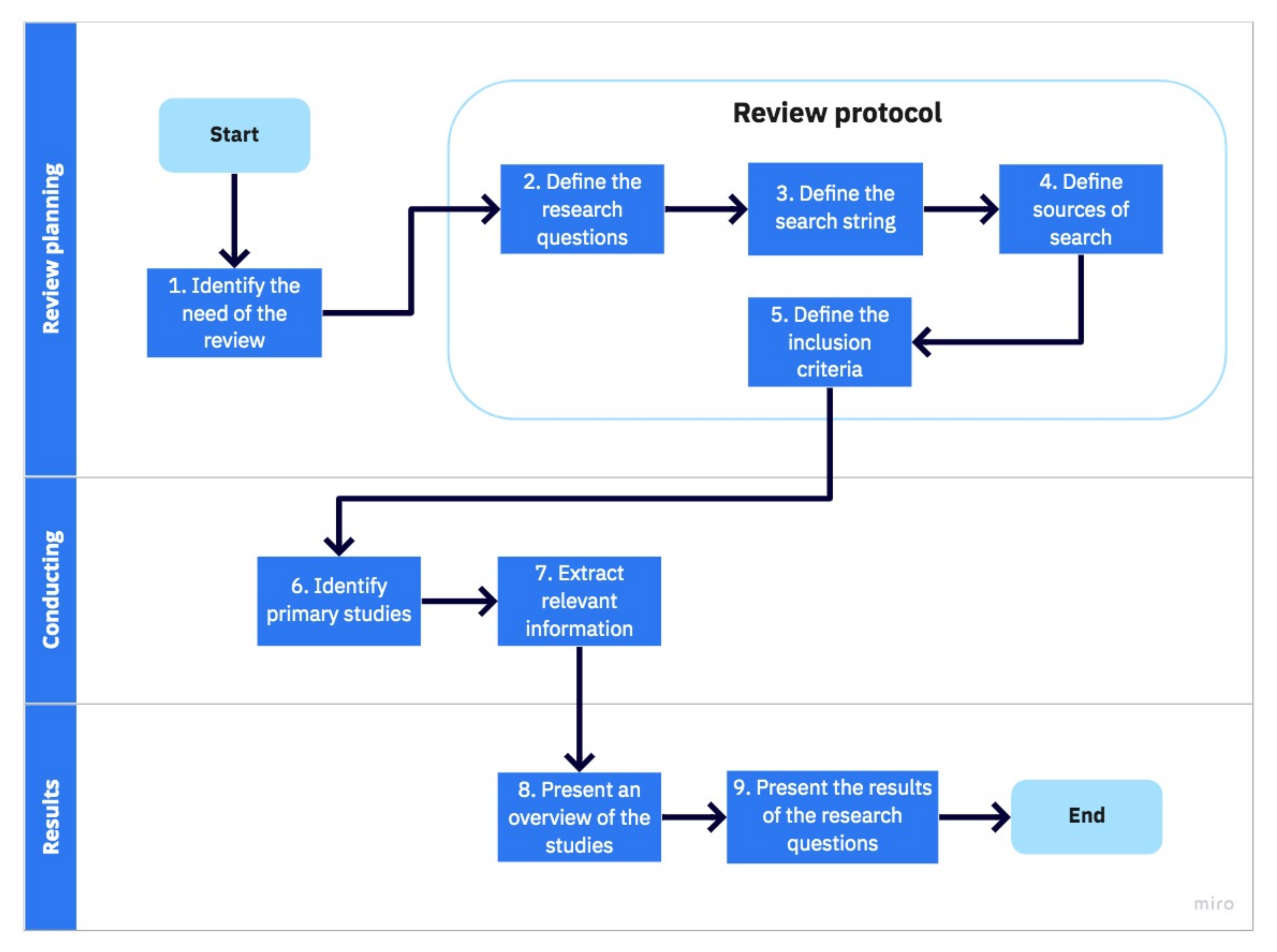
We adopted the methodology previously used by Endo et al. [15] and Coutinho et al. [16] to perform the systematic review. The mentioned systematic review protocol was originally inspired by the classic protocol that was proposed by Kitchenham [17]. Figure 1 illustrates the methodology that was adopted in this work. Next, we explain each of these steps.

Identify need of review: because of the growth of image and big data applications, both academia and industry use deep learning to analyze data and extract relevant information. For large networks, deep learning architectures suffer drawbacks, such as high computational cost, slow convergence, vanishing gradients, and hardware limitations for training.

In this systematic review, we mainly investigate the use of the CELM as a viable alternative for deep learning architectures while guaranteeing quick-training and avoiding the necessity of gradient calculations to update the network’s weights. In recent years, CELMs have solved some of the leading deep learning issues while maintaining a reasonable quality of solutions in many applications.

Define research questions: we begin our work with the definition of four research questions (RQ) that are related to our topic of study. Our objective is to answer these research questions to raise a discussion of the current state of the art in the usage of the CELM in the specific domain of image analysis. The research questions are as follows:

• RQ 1: What are the most common problems based on image analysis and datasets analyzed in the context of the CELM?
• RQ 2: How are the CELM architectures defined in the analyzed work?
• RQ 3: Which are the main findings when applying the CELM to problems based on image analysis?
• RQ 4: What are the main open challenges in applying the CELM to problems based on image analysis?

Define search string: to find articles related to our RQs, it was necessary to define a suitable search string to be used in the adopted search sources. To create such a search string, we defined terms and synonyms related to the scope of this research. The search string that was defined was "(("ELM" OR "extreme learning machine" OR "extreme learning machines") AND ("image recognition" OR "image classification" OR "object recognition" OR "object classification" OR "image segmentation"))".

Define sources of research: we adopted the following traditional search sources (databases) to find articles: IEEE Xplore (https://www.ieeexplore.ieee.org/), Springer Link (https://link.springer.com/), ACM Digital Library (https://dl.acm.org/), Science Direct (https://www.sciencedirect.com/), SCOPUS (https://www.scopus.com/), and Web of Science (https://www.webofknowledge.com).

Because we considered the four primary databases (IEEE Xplore, Springer Link, ACM DL, and Science Direct) and two meta-databases (SCOPUS and Web of Science), we first selected the articles from the primary databases because the meta-databases provided some duplicate results.

Define criteria for inclusion and exclusion: we defined criteria for the inclusion and exclusion of articles in this systematic review with the aim of obtaining only articles within the scope of this research. The criteria were, as follows:

• primary studies published in peer-reviewed journals or conferences (congress, symposium, workshop, etc.);
• work that answers one or more of the RQs defined in this systematic review;
• work published from 2010 to 2020;
• work published in English; and,
• work accessible or freely available (using a university proxy) from the search sources used in this project.

Identify primary studies: we identified the primary studies according to the inclusion and exclusion criteria.

Extract relevant information: we extracted relevant information from the primary studies by reading the entire paper and answering the RQs.

Present an overview of the studies: in this step, we present a general summary of the primary studies that were selected in the systematic review. The overview information includes the percentage of the year of publication of the articles and the database from which they were obtained. Section 3 presents the overview of the studies.

Present the results of the research questions: considering the research questions, we present the answers found from the analysis of the selected articles. The answers to the defined research questions are the main contribution of this systematic review. Section 4, Section 5, Section 6 and Section 7 present the results of this step.

3. Overview of the Primary Studies

Table 1. Search results obtained before and after refinement by inclusion and exclusion criteria.

Database	Original Search	After Primary Studies Identification
ACM DL	91	3
IEEE Xplore	123	19
Science Direct	54	6
Springer Link	992	30
SCOPUS	616	19
Web of Science	344	4

presents the number of studies before and after applying the inclusion criteria. A total of 2220 articles were returned from the six databases. After removing duplicate articles and applying the inclusion criteria, 81 articles remained, which corresponded to 3.74% of the total articles that were found in the search.

We selected 30 papers from Springer Link, and this was the database with the most primary studies returned. IEEE Xplore returned the second-highest number of primary studies, at 19. Science Direct and ACM returned six and three studies, respectively. Additionally, we can see the importance of using meta-databases in this study, as the meta-databases also returned important studies (19 from SCOPUS and four from Web of Science).

Regarding the primary studies identified, Figure 2 illustrates the percentage of publications of these studies per year. Although we established a time range between 2010 to 2020, articles on the CELM began to be published in 2015. A probable explanation for this is that the first consolidation of DL in the literature and multimedia applications, in general, was in this year. During this consolidation, several alternatives to conventional CNNs were proposed, such as a CNN with many layers [18], residual CNN networks [19], networks with batch normalization [20], dropout [21], and other advances [22]. Besides, researchers aimed to find alternatives with a better generalization capacity and better training and classification time when CELM variations were proposed. The next sections present the analysis and discussion of each research question proposed in this systematic review.

4. Common Problems and Datasets

From the primary studies, the main machine learning problems for multimedia analysis can be divided into two main groups: image classification and semantic segmentation.

Eighty studies were found to be related to image classification. Image classification is the process of labeling images according to the information present in these images [2], and it is performed by recognizing patterns. The classification process usually analyzes an image and associates it with a label describing an object. Image classification may be performed through manual feature extraction and classical machine learning algorithms or deep learning architectures, which learn patterns in the feature extraction process.

Only one study [23] covered semantic segmentation. Semantic segmentation in images consists of categorizing each pixel present in the image [4]. The learning models are trained from ground truth information, which are annotations equivalent to each pixel’s category pertinence of the input image. This model type’s output is the segmented image, with each pixel adequately assigned to an object.

The triviality of implementing the CELM models for the first purpose is the factor that may explain the high difference in the number of studies for image classification instead of semantic segmentation. For the image classification task, the architectures are stacked with convolutional layers, pooling, and ELM concepts placed sequentially (see more details in RQ 2). This fact facilitates the implementation of the CELM models.

Models for semantic segmentation need other concepts to be effective. In semantic segmentation, it is necessary to make predictions at the pixel level, which requires the convolution and deconvolution steps to reconstruct the output images. These concepts may be targeted by researchers in the future.

Note that object detection is also a common problem in the computer vision field, but we did not find studies solving object detection using CELM concepts in this systematic review.

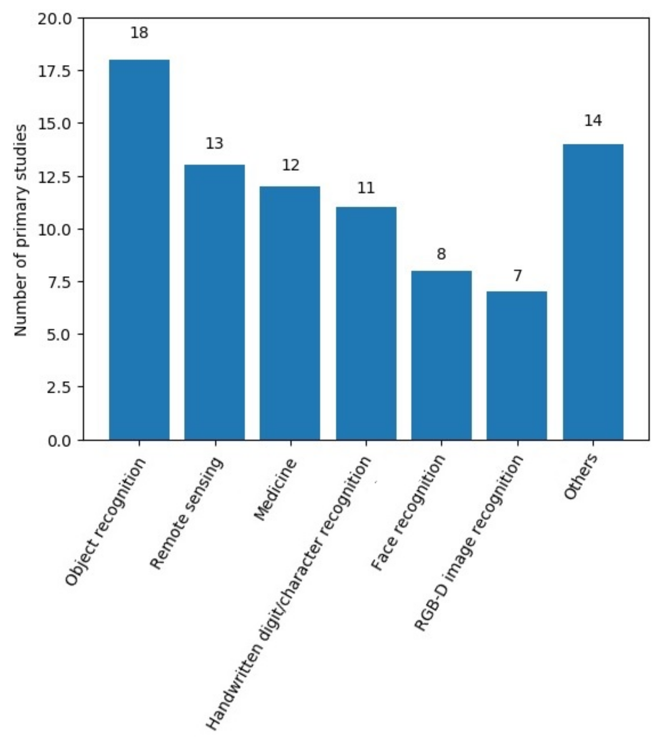
We found 19 different scenarios from the primary studies, but most of them contained four or fewer related studies. Thus, we highlight the six main application scenarios, and the others are demarcated in a single group (Others), as shown in Figure 3. The six main CELM application scenarios that were found among the primary studies were object recognition, remote sensing, medicine, handwritten digit recognition, RGB-D image recognition, and face recognition, totaling 69 articles, or about 83% of the total primary studies.

4.1. Object Recognition

Object recognition is one of the most common problems addressed in the primary studies found in this systematic review. Object recognition consists of classifying objects in scenes and it is not a trivial task. Generally, the dataset that makes up an object recognition problem comprises several elements divided by classes. The variation is realized in the object positions, lighting conditions, and so on. We found 18 studies dealing with object recognition—approximately 21% of the primary studies.

Among the primary studies, we found nine different object recognition datasets: NORB, CIFAR-10, CIFAR-100, Sun-397, COIL, ETH-80, Caltech, GERMS, and DR. These datasets, in general, have a wide range of classes, hampering the ability to generalize machine learning models. Therefore, if a proposed model obtains expressive results using large datasets for object recognition, there is strong evidence that this model presents a good generalization capacity.

Table 2. Datasets for object recognition reported in the primary studies.

Dataset	References
NORB	[6,24,25,26,27,28,29,30]
CIFAR-10	[24,27,29,31,32,33,34,35]
CALTECH	[28,35,36,37]
COIL	[25,29,34]
CIFAR-100	[33,35]
ETH-80	[25,34]
SUN-397	[33]
GERMS	[38]
DR	[39]

shows the reported datasets for object recognition and their respective references. Most of the studies use the NORB and CIFAR-10 datasets (representing more than 50% of usage). Note that some studies use more than one dataset for training and testing their models. Next, we present a brief description of the main datasets that are found for object recognition.

The NYU Object Recognition Benchmark (NORB) dataset [40] is composed of 194,400 images that are pairs of stereo images from five generic categories under different angles, light setups, and poses. The variations consist of 36 azimuths, nine elevations, and six light setups.

The Canadian Institute For Advanced Research (CIFAR-10) [41] is a dataset that contains 60,000 tiny images of $32\times 32$ in size divided into 10 classes of objects, with 6000 images per class. Additionally, CIFAR-100 contains 100 classes of objects, with 600 images per class. The default split protocol is 50,000 images for the train and 10,000 for the test set.

The Columbia University Image Library (COIL) [42] is an object image dataset. There are two main variations: COIL-20, a dataset that contains 20 different classes of grayscale images; and, COIL-100, which contains 100 classes of colored images. A total of 7200 images compose the COIL-100 dataset.

Caltech-101 [43] is a dataset that contains 101 categories. There are 40 to 800 images per class, and most of the categories contain about 50 images with a size of $300\times 200$. The last version of the dataset is Caltech-256, which contains 256 categories and 30,607 images.

ETH-80 [44] is a dataset that is composed of eight different classes. Each class contains 10 object instances, and 41 images comprise each instance. There is a total of 3280 images in the dataset.

4.2. Remote Sensing Classification

Remote sensing is information from a geospatial area acquired at a distance. The most common examples of remote sensing classification data are spectral images, which are different from ordinary RGB images, since they carry data about infrared, ultraviolet, and so on. With this type of information, it is possible to obtain a more detailed mapping of a remote sensing area. The other variation of data for remote sensing is called hyperspectral imaging [45], which, in addition to spectrum information, also considers digital photographs. The CELM has been used as an alternative solution in remote sensing classification because deep learning models generally require high processing power for this type of application. In this systematic review, we reported a total of 13 studies that applied the CELM for remote sensing classification.

Table 3. The datasets for remote sensing classification reported in the primary studies.

Dataset	References
Pavia	[46,47,48,49,50,51,52,53]
Indian Pines	[46,47,48,50,51,54]
Salinas	[46,47,49,53]
MSTAR	[55,56]
UCM	[57]
AID	[57]
R+N	[57]

shows the seven datasets used for remote sensing classification found in our primary studies. The two main datasets were Pavia (eight studies) and Indian pines (six studies), comprising about 60.9% of the total. The other datasets were Salinas, MSTAR, UCM, AID, and R+N. Next, we present a brief description of the main datasets.

The Pavia dataset [58] is composed of nine different classes of scenes that were obtained by the ROSIS sensor (https://www.uv.es/leo/daisex/Sensors/ROSIS.htm), and the total number of spectral bands is 205. In the dataset, there are images with sizes of $1096\times 1096$ pixels and $610\times 610$ pixels.

The Indian Pines dataset [58] consists of scenes that were collected by the AVIRIS sensor (https://aviris.jpl.nasa.gov/). The data size corresponds to $145\times 145$ pixels and there are 224 bands of spectral reflectance. The Indian Pines scenes contain scenes of agriculture and forests. There is also an immense amount of geographic data on houses, roads, and railways.

Like the Indian Pines dataset, the Salinas dataset [58] was collected by the 224-band AVIRIS sensor. The Salinas dataset contains a high spatial resolution with 3.7 meter pixels. The area covered comprises 512 lines by 217 samples. The dataset contains 16 ground-truthed classes.

Moving and Stationary Target Acquisition and Recognition (MSTAR) is a dataset [59] that contains baseline X-band SAR imagery of 13 target types plus minor examples of articulation, obscuration, and camouflage. The Sandia National Laboratory collected the dataset and Defense Advanced Research data [60].

4.3. Medicine Applications

There has been an increase in the number of machine learning applications for medicine. Most of them aim to identify patterns in imaging examinations to support (not replace) the specialist. Generally, the data used are labeled by medical specialists in the study field of the disease to be identified. Applications of the CELM models are made possible because they often surpass traditional models in the classification stage. All 12 studies that were found in this systematic review aimed to provide support for decision-making in diagnosing various diseases.

Table 4. Applications in medicine and their datasets reported in the primary studies.

References	Approach	Dataset
[64]	Classification of digestive organs disease	Own dataset
[65]	Liver tumor classification	Elazig University Hospital
[66]	White blood cell detection	BCCD dataset
[67]	Histopathological image classification	ADL dataset
[68]	Cerebral microbleed diagnosis	Own dataset
[69]	Cervical cancer classification	Herlev dataset
[61]	Brain tumor classification	CGA-GBM database
[70]	Micro-nodules classification	LIDC/IDRI dataset
[62]	Brain tumor classification	Brain T1-weighed CE-MRI dataset
[63]	Brain tumor classification	Brain tumor MRI dataset
[71]	Classification of anomalies in the human retina	Duke and HUCM datasets
[72]	Hepatocellular carcinoma classification	ICPR 2014 HEp-2 cell dataset

shows the 12 applications of the CELM for medicine reported in the primary studies returned, including tumor classification, anomalies detection, white blood cell detection, and so on. Brain tumor classification is the application with the largest number of studies [61,62,63]. Because of the variety of medical problems, the studies do not use a common dataset, which makes it difficult to compare them.

4.4. Handwritten Digit and Character Recognition

Similar to the object recognition problem, the handwritten digit and character recognition problem recurs in digital image processing and pattern recognition benchmarking [73]. Several studies have proposed digit and character recognition for applications, such as handwriting recognition [73]. Handwritten digit or character recognition can be applied to several tasks: text categorization from images, classification of documents, signature recognition, etc. In this systematic review, we found 11 primary studies that applied CELM in the context of handwritten digit or character recognition.

Table 5. The datasets for handwritten digit or character recognition reported in the primary studies.

Dataset	References
MNIST	[24,27,28,29,30,34,74,75,76,77]
USPS	[27,29,30,76,77]
EMNIST	[10]

presents the datasets used for handwritten digit recognition found in our systematic review. MNIST and USPS were the two main datasets for digit recognition, and EMNIST was the main dataset used for character recognition. Next, we present a brief description of the two main datasets.

The Modified National Institute of Standards and Technology (MNIST) [78] dataset contains 70,000 images that correspond to handwritten numeric figures. It is a variation of a more extensive database, named NIST, which contains more than 800,000 images with handwritten characters and numbers provided by more than 3600 writers. The MNIST contains representative images of 10 classes (digits 0 to 9) with dimensions of $28\times 28$.

The US Postal (USPS) dataset [79] is composed of digital images of approximately 5000 city names, 5000 state names, and 10,000 ZIP codes, and 50,000 alphanumeric characters are included. The images have a size of $16\times 16$.

4.5. Face Recognition

Face recognition is commonly present in security systems, tagging people on social networks, etc. It is also common for several machine learning models to use face recognition databases as benchmarking [80]. We found eight studies that cover object recognition, comprising about 9% of the primary studies.

Table 6. The datasets for face recognition that were reported in the primary studies.

Dataset	References
YALE	[26,28,81]
ORL	[26,29]
Casia-V4	[82]
CMU-PIE	[30]
XM2VTS	[81]
AR	[81]
LFW-a	[81]
FERET	[81]
Youtube-8M	[83]
ChaLearn	[84]

presents the 11 datasets that are used for face recognition with CELM models found in our systematic review. The YALE dataset was the most used, while ORL was used in two studies.

The YALE dataset [85] contains 165 images from 15 different people, with 11 images for each person. Each image contains different expressions, such as happy, sad, sleeping, winking, etc.

The ORL face dataset [86] is composed of 400 images with a size of $112\times 92$. There are 40 persons, with 10 images per person. Like the YALE dataset, there are different expressions, lighting setups, and so on.

4.6. RGB-D Image Recognition

RGB-D images are graphical 3D representations of a capture that may be used for object recognition, motion recognition, and so on. In addition to RGB color images, another channel (-D) of information that corresponds to depth is added. It is possible to obtain accurate information on the shape and location of the objects analyzed on the scene. The low-cost Microsoft Kinect sensor is generally used to capture scenarios and objects. With that, several machine learning models are currently used for object recognition [87] and human motion [88], among other applications using data from RGB-D sensors [89]. Seven studies applied CELM models for the learning process for RGB-D data, representing 8% of the primary studies.

Table 7. The datasets for RGB-D image recognition reported in the primary studies.

Dataset	References
Washington RGB-D object	[90,91,92,93,94,95]
2D3D object	[94]
Sun RGB-D object	[94]
NYU indoor scene	[94]
Princeton ModelNet	[96]
ShapeNet core 55	[96]
Princeton shape benchmark	[96]
MIVIA action	[97]
NOTOPS	[97]
SBU Kinect interaction	[97]

presents the datasets that are used for RGB-D image recognition found in our systematic review. The Washington RGB-D object was the most used dataset. All of the other databases were used by only one work: 2D3D object, Sun RGB-D Object, NYU Indoor Scene, Princeton ModelNet, ShapeNet Core 55, Princeton Shape Benchmark, MIVIA action, NOTOPS, and SUB Kinect interaction. Next, we present a brief description of the main dataset: the Washington RGB-D.

The Washington RGB-D Object dataset [98] contains 300 objects that were captured by a Kinect camera with a $640\times 480$ resolution. The objects are organized into 51 categories. The captures are sequential; that is, three video sequences for each object were recorded.

4.7. Other Application Scenarios

We also found studies involving scenarios with fewer applications, such as street applications, factories, food classification, textures, documents, etc.

Table 8. Other application scenarios found in the primary studies.

Application	References
Food classification	[31,35,99,100]
Street applications	[101,102,103]
Factory	[104,105,106]
Motion recognition	[107,108,109]
Detection	[24,110]
Texture classification	[26,111]
Image Segmentation	[23]
Document recognition	[112]
Criminal investigation	[113]
Animal classification	[35]
Robotics	[114]
Fire detection	[115]
Clothes classification	[116]

summarizes the complete list of other applications that are found in this systematic review’s primary studies.

5. CELM Architectures

From the primary studies, we can define two main categories of CELM usage: (i) studies that use a CNN for feature extraction and the ELM for fast learning on extracted features and (ii) studies that use the ELM for the fast training CNN architectures. Both of the approaches can improve training time and multimedia data learning tasks. Figure 4 illustrates a summarization of how CELMs are being used in the current literature.

In the CNN for feature extraction and the ELM for fast learning on extracted features, the power of representation of the inputs increases with deep features, and the ELM enables a shorter training time and a high capacity for generalization [6]. There are some variations of this approach: (i) a CNN can be used for feature extraction using predefined kernel weights (or filters), in which classic image and signal processing filters are used (see Section 5.1); and, (ii) a CNN can be used for feature extraction using previously pre-trained weights, in which the pre-trained weights can be learned in the same or different application domains (see Section 5.2 and Section 5.3).

The usage of ELM concepts for the fast training of classical CNN architectures involves using a complete CNN, substituting the training process (see Section 5.4). The training is no longer done by backpropagation, but by algorithms that are based on the ELM to learn the features. This change provides a better training time for CNN and it leads to further improvements.

Figure 5 presents the amount of work for each type of CELM usage. More than half of the primary studies used a CNN with pre-defined filters to extract features and an ELM to train the features (about 54%). The other three types of CELM architectures were distributed in similar quantities. In the following subsections, we discuss how the primary studies applied these different CELM architectures.

5.1. CNN with Predefined Kernels for Feature Extraction and ELM for Fast Learning

This approach was the broadest and most varied when compared to the others. This is because there are many architectures that are based on default kernel (or filter) initialization. In this approach, CNNs are used as feature extractors without any prior training and the fully connected layer CNN kernels are pre-defined through processing, statistical distribution, or the decomposition of values, whereas ELMs or their variations replace fully connected layers. In this approach, the architecture removes backpropagation training and makes the learning process more simple. Figure 6 shows a generic example of this architecture.

Several kernels can be used in the convolution layers, such as Random, Gabor, PCA, Patch, and even a combination of these. Some studies have also proposed techniques for the pre and post-processing of the convolutional layers’ features.

Table 9. Variations of works using CELM with pre-defined kernels. * Note that there are works based on CNN with random filters + ELM, which we consider as a special case, named ELM-LRF, and therefore are referred to specifically in Table 10.

Approaches	References
CNN with random filters + ELM *	[33,47,56,62,72,75,76,92,97,99,109]
CNN with gabor filters + ELM	[48,104]
CNN with a combination of filters + ELM	[10,107]
Ensemble of CNN with predefined filters + ELM	[55,72,75]
Combination of image processing techniques + CNN with predefined filters + ELM	[23,55,92,117]
PCANet + ELM	[71,81]

summarizes the studies that used CELM with pre-defined kernels from the primary studies. Note that some of the studies used more than one approach.

5.1.1. Random Filter

The most used kernel found in the primary studies was the kernel randomly generated through a Gaussian distribution, or the random filter: [33,47,56,62,72,75,76,92,97,99,109].

There is a particular case of a CELM where the CNN has random, but orthogonalized, filters, known as the local receptive field-based extreme learning machine (ELM-LRF). Huang et al. [6] proposed the ELM-LRF, and it is based on the premise that ELM networks can adapt themselves and achieve good generalization when random features are used that represent local regions of the input images. The use of the LRF term comes from CNNs, as they can represent different regions of a given image through their convolutions. The network structure consists of a convolutional layer, followed by pooling, while an ELM network is responsible for the training and classification of the extracted features. The convolution kernels are orthogonalized, employing decomposition by singular values (SVD). The convolutional layer applies random filters to extract the LRF. Square-root pooling is applied to reduce the dimensionality of the data. Finally, all of the traditional learning is performed through the ELM network to calculate the inverse Moore–Penrose matrix to train the features that are generated by the LRF. There is no hidden layer with random weights in the classifier, only one layer of output weights.

Several studies have applied the ELM-LRF in its default form for their learning process [6,25,39,52,53,63,90], along with some other variations of ELM-LRF, as shown in

Table 10. Variations for ELM-LRF reported in the primary studies.

Approach	References
ELM-LRF (default)	[6,25,39,52,53,63,90]
Multimodal ELM-LRF	[55,91,93,105]
Multiple kernel ELM-LRF	[26]
Multilayer ELM-LRF	[27,38,51,67,77,114]
Autoencoding ELM-LRF	[27,28,93]
Multiscale ELM-LRF	[67,106,111]
Recursive ELM-LRF	[29]

.

Some of the studies considered using multiple data sources for parallel feature extraction with the ELM-LRF to make a unique final decision. These approaches that consider multiple data sources are named as multimodal [55,91,93,105].

We previously presented some studies that combined different filters in CNNs for feature extraction. This feature combination approach is also used in the ELM-LRF architecture of multiple kernel ELM-LRF [26]. In this work, the authors proposed using a variation of Gabor filters with random filters and, for this reason, the authors named this approach ELM-hybrid LRF (HLRF). The authors carried out experiments to define the p and q values of the Gabor filters and performed an analysis of the number of layers that provided optimal accuracy values.

The multilayer ELM-LRF is another known ELM-LRF variation that consists of multiple convolution and pooling layers [27,38,51,67,77,114].

Autoencoding ELM-LRF leads to high-level feature representation using ELM-AE with the ELM-LRF and it was proposed by [27,28,93]. Another notable difference is the use of three ELM-AEs in parallel for each respective color channel for coding features. The work [93] proposed a Joint Deep Random Random Convolution and ELM (JDRKC-ELM) model for the recognition of two data modalities separately (an application of the ELM-LRF). After feature extraction, the fusion layer that used a coefficient to combine two feature types and ELM-AE learned top-level resource representations. The ELM classifier is responsible for the final decision.

Furthermore, some studies considered all the channels or variate scales (multiscale) of the images by applying different ELM-LRF architectures for feature extraction and learning tasks [54,67,106,111].

Furthermore, to conclude the ELM-LRF variations, Song et al. [29] presented two recursive models based on the ELM Random Recursive Constrained (R2CELM) and ELM based on Random Recursive LRF (R2ELM-LRF), which are constructed by stacking CELM and ELM-LRF, respectively. Following the concept of stacking generalization, random projection and kernelization were incorporated in the proposed architectures. R2CELM and R2ELM-LRF not only fully inherit the merits of ELM, but also advantage of the superiority of CELM and ELM-LRF in the field of image recognition, respectively. R2CELM and R2ELM-LRF demonstrated their best performance in precision tests on the six sets of reference image recognition data in the empirical results.

5.1.2. Gabor Filter

The studies in [48,104] used the Gabor filter, which is considered to be similar to the human visual system, and it is widely used in general computer vision tasks, not only in CNNs. The Gabor filter is linear, and it is generally used for analyzing textures in images. Frequency and orientation attributes are used in Gabor filters. Similar to the random filter, the Gabor filter that was used in [48,104] obtained a high capacity to represent the data and it could provide a better generalization of ELM.

5.1.3. CNN with Combination Filters

Other studies used a combination of different filters in the convolutional layers. In [10], the authors observed that CELM approaches in the literature have the limitation of using random filters in only one step of extracting features. Because of the random filtering usage limitation, the authors propose the combination of the following filters: random filter, patch filter (sub-regions were chosen from an input image), principal component analysis (PCA) filters, and the Gabor filter. In [107], the authors apply the Gabor filter with different values of directions and scales in the first convolutional layer, and the Radial Basis Filter is applied in the second convolution layer. After each convolution layer, the data are pooled by pooling layers. Both of the approaches provide a good generalization capacity.

5.1.4. Ensemble of CNN with Pre-Defined Filters

Ensemble approaches of CNNs and ELMs have been considered in [55,72,75]. An ensemble generally consists of a combination of more than one learning model for a final decision [118]. Figure 7 illustrates an example of an ensemble of the CELM.

In [75], the authors use three CELM architectures combined with the majority voting ensemble. Each sub-architecture consists of three convolutional layers, with each one followed by a pooling layer; then, at the end, an ELM is responsible for the training and classification process. In [72], the authors train three different ELM networks for the classification process. Each ELM network has, as an input, the last two convolutional layers and last pooling layer, and an ensemble makes the final decision for these three ELMs. The work that was presented in [55] was described previously in a multimodal ELM-LRF.

5.1.5. Combination of Image Processing Techniques and CNN with Pre-Defined Filters

In addition to convolutions, pooling, and ELM, some studies also consider image processing techniques for the pre and post-processing of images or features: [23,55,92,117]. The authors in [92] propose using K-means in the inputs; then, convolution filters are applied. Spatial Pyramid Pooling and a recursive neural network are applied to the abstraction of the data that were generated before applying the ELM for training and classification. In the end, the ELM is used for feature learning and classification. The approach proposed in [55] consists of the feature extraction by CNN in two types of input: (i) the original image and (ii) the image after the transformation of rotation through fractal extraction and segmentation. After that, the features are combined and trained by two ELM networks. The final decision is made by combining the outputs of these ELMs. In [23], the authors propose the extraction of superpixels using the Simple Linear Iterative Clustering (SLIC) algorithm. With that, the extraction of candidate regions with their corresponding labels is completed. The CNN architecture is applied in these candidate regions for feature extraction, so that the ELM performs the prediction of semantic segmentation in the images. In [117], the image data are captured, and a search is done for color similarity in the image. After that, segmentation is applied. Finally, two convolutional layers are applied, with each one followed by two pooling layers. With that, the data are classified by a KELM (a ELM with an RBF kernel).

5.1.6. PCANet

The work in [71] presents a classification approach that consists of using the PCANet [119] network to extract features using the Principal Component Analysis (PCA) algorithm in convolutions in the images. Subsequently, the ELM with the composition of several kernels is used for the classification task. The proposed approach presents promising results. The work in [81] develops a new approach for image classification using a new architecture, the 2DPCANet—a variant of PCANet. While the original PCANet network performs 1D transformations for each image line, the 2DPCANet performs 2D transformations in the entire image. As a result, there is a refinement in the process of extracting features. At the end of the feature extraction, the training with the ELM network is carried out. The architecture is evaluated in a different dataset and it shows improved accuracy when compared to the original architecture.

We observed that all studies in this section use small CNN architectures. The authors usually do not specify how to define the ideal number of layers and filters. When the number of layers and filters is increased, the amount of data to be processed by ELM also increases. In the literature, classic machine learning algorithms tend to perform the learning task with more difficulty when dealing with a vast amount of data. Besides, the computational processing time increases in proportion to the complexity of the CNN architecture. For the reasons that are mentioned above, several studies have proposed simpler CNN architectures for extracting characteristics, as the objective is to obtain maximum accuracy without gradually increasing the computational cost.

5.2. Pre-Trained CNN in Other Application Domain for Feature Extraction and ELM for Fast Learning

It is necessary to have large amounts of data and machines with a tremendous computational capacity to train deep learning models. Machines with dedicated hardware with GPU processing can be used for training such models, but large amounts of data or resources may not be available for the creation of the models. Therefore, the concept of transfer learning was proposed to deal with these problems.

In transfer learning, the knowledge learned to perform one task can be used to perform another task [120]. In this process, the features that one model has learned to perform a task can be transferred to another model to perform a different task. A minor adjustment (named fine-tuning) needs to be performed on the last layers of the model (usually the fully connected layers) [121]. In this systematic review, we reported studies that propose a fine-tuning approach using an ELM-based classifier. This approach is similar to the previous ones that were reported in Section 5.1. The difference is that a pre-trained CNN (generally without the fully connected layers) is used to perform the feature extraction process. An ELM-based classifier is used to make a new training process with the extracted features. Note that we name this process as fine-tuning with ELM. Figure 8 illustrates the transfer learning process with an ELM.

We found various studies that use classic deep neural architectures for a transfer learning task, such as AlexNet, CaffeNet, VGGNet, GoogLeNet, Inception-V3, ResNet, and SqueezeNet. Furthermore, their own deep pre-trained architectures have been proposed in some studies for the transfer learning task.

Table 11. The pre-trained architectures used for fine tuning with ELM reported in the primary studies.

Pre-Trained Architecture	References
AlexNet	[57,113]
CaffeNet	[69,101,122]
VGGNet	[31,57,66,68,69,83,96,100,115]
GoogLeNet	[57,66,82]
Inception-V3	[31]
ResNet	[31,66,96,100,115]
SqueezeNet	[61]

summarizes the studies that use pre-trained deep learning architectures and fine-tuning using an ELM.

AlexNet is the first deep learning architecture used for transfer learning and fine-tuning with an ELM that we cover [123]. The AlexNet architecture is one of the pioneers responsible for popularizing deep learning for image recognition. This architecture has five consecutive convolutional layers with a filter size equal to 11 and pooling. After each convolutional layer, the Rectified Linear Unit (ReLU) activation is used to reduce the classification error. Three fully connected layers are responsible for data classification. AlexNet was initially trained in the ImageNet Large-Scale Visual Recognition Challenge (ILSVRC) dataset using multiple GPUs. The authors adopted the freezing part of the weights (dropout) and data augmentation to overcome the overfitting problem. The architecture reached an error of 15.3% in the database used in the year 2012, and it was much higher than other architectures. With all of the acquired learning, the architecture is used to extract characteristics and then remove the fully connected layers.

Some studies used the AlexNet architecture with the pre-trained weights in the ILSVRC dataset in conjunction with ELM networks to replace fully connected layers, thus achieving fine-tuning [57,113]. There is a variation of the AlexNet model that uses a unique GPU for training task, and the variation is named CaffeNet [124]. The CaffeNet model with pre-trained weights in the ILSVRC dataset was also used for feature extraction and fine-tuning with an ELM [69]. Using CaffeNet, the studies [101,122] presented a new architecture considering the canonical correlation between visual resources and resources based on biological information. The use of discriminative locality-preserving canonical correlation analysis (DLPCAA) was adopted after the feature extraction stage, when considering the information on the label and preserving the local structures for calculating correlation. In the second layer, training with ELM was performed, which does not need many images for training.

VGGNet is another important classic deep learning architecture used for fine-tuning with an ELM [18]. There are variations of VGGNet, such as VGG-16 and VGG-19, which contain several characteristics in common, such as the number of convolutional layers being varied, all containing three fully connected layers. Firstly, the use of smaller local receptive fields with kernel sizes equal to three stands out, unlike AlexNet, which has sizes of 11. VGGNet architectures have five blocks of convolutional layers with ReLU and pooling, and the number of filters varies from 64 to 512. The architecture has many convolutional layers that can increase the data representation capacity and successfully transfer learning applications.

We reported the use of VGG-16 [31,57,66,68,69,115] and VGG-19 [100] architectures for extracting features and fine-tuning with ELM; all of the previously mentioned studies used pre-trained weights from the ILSVRC dataset. The work [83] presented an approach to predict and classify data using a multimodal approach, where video data (frame sequencing) and audio are considered. The image data were extracted with the VGG-16 and the audio data were processed with LSTM. Finally, the data were trained and classified with an ELM. The authors in [96] presented a computationally efficient method for image recognition. A new structure of multi-view CNNs and ELM-AE was developed that uses the composite advantages of the VGG-19 deep architecture with the robust representation of ELM-AE features and the fast ELM classifier.

GoogLeNet and Inception-V3 are other pre-trained CNN in the ILSVRC database for feature extraction and fast learning with ELM. The GoogLeNet architecture [125] makes use of $1\times 1$ convolutions coupled in named Inceptions modules, which reduces the computational cost. Global average pooling is used instead of fully connected layers. This reduction by global average pooling reduces the representation of the feature maps to a single value that is directly connected with the softmax layer for class prediction. These are the studies from this systematic review that use GoogLeNet with pre-trained weights on the ILSVRC dataset to extract features [57,66,82]. Inception-V3 is an evolution of the previous model containing regularization, grid size reduction, and factorizing convolutions. Inception-V3 [126] is also considered to be a good alternative for transfer learning and it has been considered in the literature for fine-tuning with an ELM [31].

The deep residual network (ResNet) [19] was proposed for ILSVRC 2015 and it was the winner with a classification error of 3.57%. ResNet contains identity shortcut connections, which are skipping connections in convolutional layer groups. The idea behind skipping connections in ResNet is to prevent the network, which is very deep, from dying due to the gradients evolving. ResNet uses a signal that is the sum of the signal that is produced by the two previous convolutional layers plus the signal transmitted directly from the point before these layers. We found several studies that used ResNet for transfer learning using the pre-trained weights from the ILSVRC dataset in conjunction with an ELM [31,66,96,100,115].

In [127], the deep network SqueezeNet was proposed, which is also used for transfer learning with the neural network ELM. However, this architecture provided the same accuracy as AlexNet in the ILSVRC database, with fewer trained parameters. The data were compressed and processed in Squeeze layers, which were composed of 1 × 1 convolutions. The data expansion was performed through more convolutional layers with sizes of 1 × 1 and 3 × 3, expanding the local receptive fields. As a result, the architecture is simpler to process and it provides a good representation of the data. The work in [61] used SqueezeNet for feature extraction and ELM for training the extracted features. Additionally, the approach used the Super Resolution Fuzzy-C-Means (SR-FCM) clustering technique for image segmentation.

5.3. Pre-Trained CNN in Same Application Domain for Feature Extraction and ELM for Fast Learning

We previously discussed deep and transfer learning models that were applied to feature extraction and fine-tuning with ELM networks. These previously reported transfer learning models are pre-trained in another application domain. This systematic review also reports papers that use pre-trained transfer learning architectures in the same application domain. The objective then is not to decrease the computational cost (when the authors train the architectures), but rather to increase the proposed final architecture’s accuracy.

This section discusses two types of application of the approach. Firstly, some studies have been trained in the ILSVRC database and are used for fine-tuning in the same application domain as the ILSVRC. Secondly, some studies fully train architectures (classic or proprietary) and then immediately use the network to extract features in the same work for later fine-tuning with ELM. We discuss these two types of application below.

Table 12. The pre-trained architectures used for fine tuning in the same domain with ELM reported in the primary studies.

Pre-Trained Architecture	References
AlexNet	[32,36,37,112]
VGGNet	[84,94]
MobileNet	[108]
DenseNet	[35]
Own architectures	[46,49,50,64,65,70,102,103,116]

refers to the transfer learning architectures that were used in this approach.

The authors in [112] propose an approach for image classification based on a hybrid architecture of the CNN and ELM. The CNN architecture used is AlexNet with pre-trained weights from the ILSVRC dataset (the same current application domain). The work performs two stages of training: the first training stage consists of re-training the model in the same work’s database, using the complete AlexNet architecture; the second training stage consists of the usage of the trained architecture as a feature extractor. The dense layers are removed, and an ELM network replaces it, performing fine-tuning on the feature vector. As expected, the training time gains in terms of performance in the test.

The authors in [36,37] propose an approach for object recognition using a hybrid method, in which the AlexNet architecture is responsible for the training and feature extraction. Fine-tuning is done with training sets from different proposed datasets. With its variants, such as adaptive ELM (AELM) and KELM, ELM is used in the data classification stage. The KELM provides the best accuracy, which is better than the ELM, SVM, and MLP.

The work presented in [32] combines AlexNet and ELM for image classification in robots’ artificial intelligence. A CNN is used for feature extraction. As a result, the use of CNN and ELM classifiers shows a faster learning rate and a more accurate classification rate than other classification methods. The ReLU activation function is used on the ELM network, obtaining better performance than the existing classification methods.

The work shown in [94] presents an approach for image classification in a scene that is invariable from the camera’s perspective. The authors use a pre-trained convolutional neural network (VGG-f) to extract features from different image channels. VGG-f is another variation of the VGGNet architecture. The authors created the HP-CNN-T, an invariant descriptor, to further improve performance. The convolutional hypercube pyramid (HP-CNN) may represent data at various scales. The classification results suggest that the proposed approach presents a better generalization performance. In [84], the authors present a multimodal approach for regression. The approach consists of feature extraction from using the VGG-19 and VGG-face networks. The data were merged and trained with the KELM network for regression (since a probability-based estimation is made).

In terms of compact deep learning models, the MobileNet model [128] was developed to be small and adaptable for mobile devices and to use less processing power. Every standard convolution is factored into a depth-to-depth and point-wise $1\times 1$ convolution. The authors in [108] use the MobileNet model in a multimodal approach; that is, it receives data from three different types of data for the training process. Thus, the authors perform the training process on the MobileNet network for each data source. The re-trained MobileNet networks are used as feature extractors through each network’s last fully connected layer. Each set of features extracted by the different data sources are trained in three different KELM networks. Finally, the results that are generated by each KELM are combined through an ensemble-based decision rule.

DenseNet [129] is another classic deep learning architecture. Each convolutional layer of the network receives an additional input from all previous layers and then passes its feature maps and all subsequent layers. Unlike ResNet, where concatenation is in blocks via gates, each layer receives information from all previous layers. The work in [35] presents an approach to image classification using a DenseNet for training and feature extraction and KELM for fine-tuning. The authors perform the training of the DenseNet deep network in the proposed dataset. After that, the trained DenseNet is used for feature extraction. Finally, the approach uses a KELM to train the extracted features.

In contrast to the previous work, other authors proposed a different architecture instead of using a known network for the transfer learning, such as [46,49,64,102,103,116], which propose CELM architectures with a different number of convolutional and pooling layers. The authors used CNN architectures for training the data with the fully connected layers. After the training, the authors used their trained networks for feature extraction. They then used the features that were extracted in the ELM network (or its variants) for a new training process and later for data classification.

The authors in [65] presented the Perceptual Hash-based Convolutional Extreme Learning Machine (PH-C-ELM) to classify images using a three-stage hybrid. This architecture uses a convolutional network in the data that were generated by Discrete Wavelet Transform-Singular Value Decomposition (DWT-SVD) values after the feature extraction step for data sub-sampling. The authors present a fine-tuning approach, where the proposed CNN is trained in the data, and it is then used as a feature extractor. Finally, an ELM is trained with the extracted features.

The work shown in [70] presents an approach for image classification in multidimensional sliced images. The authors proposed five different CNN3D architectures (each input consisted of 20 slices per multidimensional image). The training process is conducted by fully connected layers (softmax). Each CNN architecture produces different local receptive fields and, therefore, different features. After the CNN training, the architectures are used as feature extractors, and then the features are combined for new training in an ELM.

The authors in [50] presented an architecture for image classification that employs convolution–deconvolution layers and an optimized ELM. Deconvolution layers are used to enhance deep features in order to overcome the loss of information during convolution. A full multilayer CNN is developed, which consists of convolution, pooling, deconvolution layers, ReLU, and backpropagation. Additionally, the PCA algorithm is used to extract the first principal component as a training tag. The deconvolution layer can generate enlarged and dense maps, which extract high-level refined resources. The results demonstrate that the proposed structure surpasses other traditional classifiers and algorithms based on deep learning. This is the unique result of the systematic review regarding the use of deconvolution layers.

5.4. Fast Training of CNNs Using ELM Concepts

Unlike the other aspects that have been presented so far, such as a typical CNN for feature extraction and an ELM for training the extracted data, there are also approaches that consist of using the complete training of CNNs using ELM concepts. The learning process is not based on the use of the backpropagation algorithm. ELM concepts are used to calculate the error and update the filters and weights based on the Moore–Penrose pseudo-inverse matrix. This ensures fast and efficient training, in addition to offering better data representation and generalization capabilities. Next, we present the studies that use ELM concepts for fast training.

The authors in [34] use an approach for the representation of features based on the PCANet network and ELM autoencoder. The proposed architecture aims to understand and extract features for the most diverse applications with low computational cost. Three main stages are implemented to carry out the learning process: (i) the filters and weights are obtained with an ELM autoencoder and ELM decoder with convolutional layers; (ii) a max-pooling operation is used to reduce the dimensionality of the data; and, (iii) post-processing operations, such as binary hashing and block-wise histogram, are implemented to combine the features obtained to be used in the final classification step. The authors suggest that any classifier can be used to learn the obtained features. The error results in comparison with PCANet show that the proposed model has a lower error rate in all of the evaluated scenarios, in addition to offering fast training using an ELM neural network.

The work presented in [74] proposes a convolutional neural network model with training being inspired by an ELM. The convolutional network consists of only two layers, convolutional and pooling, disregarding the fully connected layers. A convolutional layer replaces the fully connected layers with a 1 × 1 kernel, similar to the GoogLeNet. The steps for modeling and training the proposed network are followed by applying convolution filters in all image regions, forming $n\times n$ window matrices. A reshape is applied to each window, and the filters are learned with an ELM-based approach. This approach provides a calculation of the Moore–Penrose pseudo-inverse matrix and updates the weights and biases of the convolutional layers. The authors compare the proposed approach with a typical CNN with the implemented backpropagation. Although the proposed approach obtains slightly less accuracy than the baseline, it is worth considering that the training time is 16 times longer than the baseline, which indicates that it is possible to obtain high accuracy with little training time.

The authors in [24] propose a new network, named CNN-ELM, for the classification and detection of objects in images, applying the ELM concept at two levels. The first level uses ELM for training the convolutional layers. In these layers, random filters are applied together with the ELM-AE to improve these kernels through autoencoder representation. In the second level, the extracted features are classified with the multilevel ELM (ML-ELM), an ELM neural network with multiple layers, following the concepts of deep learning. The use of this architecture provides fast processing; however, this is at a high memory cost. Because of this problem, the authors propose using batches (or blocks) of data to be trained in memory. In comparison with several baseline architectures, the proposed model obtains the best accuracy and training time.

The work in [130] proposes a new architecture and a training algorithm for convolutional neural networks. The Network in Network (NIN) and ELM architecture combined with CNN is adopted, with each one’s advantages being explored in the work. This architecture naturally exploits the efficiency of extracting random and unsupervised resources, consisting of a deeper network. The image input is converted into localized patches that are vectorized. They are divided into clusters to pass through the Parts Detector (ELM), where random weights adjust the hidden layers. They are submitted to ELMConv, where random convolutional filters with a sigmoid activation function are used, returning unsupervised convolutional filters. They pass through the ReLU activation function, and an average grouping, normalization, and final classification are performed with the ELM.

In [110], the authors propose a new approach for performing object tracking using convolutional networks with a modification in the training model. The proposed CNN architecture contains two convolutional layers, followed by two layers of poolings, and there are also the traditional fully connected layers with a softmax activation function. The authors still use the descending gradient to update the network’s weights and filters with a modification. An autoencoder ELM is used to learn and update the layer weights between the first pooling layer and the second convolutional layer. This provides a reduction in training time and, consequently, a gain in performance.

The work presented in [30] proposes a new architecture, named ELMAENet, for image classification. The proposed architecture includes three layers: (i) a convolutional layer with filter learning through ELM-AE; (ii) a non-linear processing layer, where the values are binary with hashing and a histogram; and, (iii) a pooling layer. The learning of these features is performed by the ELM-AE structure. The architecture is evaluated using several datasets and compared with several models, achieving the best computational performance of the studied methods.

The authors in [131] propose an approach for image classification using the CNN and ELM. The work’s main contribution is a new method for extracting features, where convolutional layers are used with learning filters without the need for the backpropagation algorithm. The authors use ELM-AE to learn the best features in the convolutional layers. An ELM ensemble is used for the data classification. The proposed architecture is evaluated using different datasets and, in three of them, it obtains the best results in terms of accuracy.

The work [132] presents a new approach to train CNNs using ELM and applies it for image recognition. The architecture consists of three convolutional and two pooling layers. There are ELM networks between the two pooling layers and the subsequent convolution layers. There is also an ELM network to carry out the recognition stage of the tracks. The error is propagated from the last ELM network near the target (labeled image) in the opposite direction of the network until the first convolution layer is reached. From that, convolution weights, filters, and other parameters are adjusted with the intermediate ELM networks, which provides faster adjustment and learning. The proposed approach is superior to others in the literature in terms of accuracy and computational performance.

6. Main Findings in CELM

Based on the scenarios and the most common datasets used in the primary studies, in this subsection we describe the main findings when applying the CELM to image analysis.

Next, we present the accuracy results of the CELM models using the primary databases that are presented in Section 4. We also present the time that is required for training and testing the CELM models. It is worth mentioning that the presentation of these time results shows that CELM models are trained and tested in less time than classic machine learning models, and it is important not to compare them against each other, as each model was trained and tested in different machines with different setups.

The authors in [6,24,25,26,27,28,29,30] applied CELM to solve the object recognition problem using the NORB dataset. In general, all studies presented a good accuracy, with all of them achieving over 94%, as shown in

Table 13. The results obtained by CELM architectures for object recognition in the NORB dataset.

Reference	Approach	Accuracy	Training Time (s)
Huang et al. (2014) [6]	ELM-LRF	97.26	394.16
Bai et al. (2015) [25]	ELM-LRF	97.24	400.78
Yoo and Oh (2016) [24]	CNN-AE-ML-ELM	94.92	1165.87
He et al. (2019) [26]	ELM-HLRF	97.45	516.08
Wu et al. (2020) [27]	ELM-ARF	98.00	216
Wu et al. (2020) [28]	ELM-MAERF	98.53	279
Song et al. (2020) [29]	R${}_2$ELM-LRF	97.61	4401.07
Chang et al. (2020) [30]	ELMAENet	98.28	-

. All of these studies performed comparisons against algorithms, such as the classic CNN, MLP, and SVM, and the CELM models outperformed all of the studied approaches.

The best accuracy results were 98.53%, and 98.28%, which were achieved by [28] using an ELM-LRF with autoencoding receptive fields (ELM-ARF) and [30] using the ELMAENet, respectively. This demonstrates the excellent representativeness of the extracted features and generalization capability of ELM models.

In general, we noted that some of the studies only presented the training time in the papers for the NORB dataset in their experiments. For this reason, in Table 13, we do not consider testing time in the discussion. The best training time was achieved by [27] (216 s), and this result was probably due to the compact autoencoding features by ELM-AE. The worst result was achieved by [29] (4401.07 s). The difference may probably be due to the different machine and scenario setup, as previously discussed. In general, ELM-LRF-based architectures provide a low training time due to the simplicity of the architectures. All of these architectures presented better training results than classic machine learning models.

The authors in [46,47,48,49,50,51,54] used the Pavia dataset for remote sensing classification. Note that remote sensing approaches use other evaluation metrics, such as average accuracy (AA), overall accuracy (OA), and Kappa, as shown in

Table 14. Results obtained by CELM architectures for remote sensing classification in the Pavia dataset.

Reference	Approach	AA	OA	Kappa	Training Time (s)	Testing Time (s)
Lv et al. (2016) [51]	ELM-HLRF	98.25	98.36	0.981	44.12	-
Shi and Ku (2017) [48]	CNN(gabor)-ELM	94.3	92.8	0.940	-	-
Shen et al. (2017) [54]	ELM-LRF	97.95	98.29	0.981	-	-
Li et al. (2018) [50]	CNN(pre-trained)-ELM	-	96.70	0.955	-	-
Cao et al. (2018) [49]	CNN(pre-trained)-ELM	97.50	98.85	0.983	-	-
Huang et al. (2019) [46]	CNN(pre-trained)-ELM	85.50	87.77	0.860	14.10	25.24
Shen et al. (2019) [47]	CNN(random)-ELM	-	97.42	0.971	49.00	0.79

.

The most common approach used for this purpose is a CNN that was previously pre-trained in the Pavia dataset used for feature extraction and an ELM for the classification task [46,49,50]. However, the ELM-HLRF thatwas proposed in [51] achieved the best AA and OA results, at 98.25% and 98.36%, respectively.

Most of the studies did not report any results regarding the training or testing time, but we show the effectiveness in these metrics for remote sensing classification. The work in [46] reported a low training time of 14.10 s, and the work in [47] achieved 0.79 s of testing time.

Table 15. Results obtained by CELM architectures for handwritten digit recognition in the MNIST dataset.

Reference	Approach	Accuracy	Training Time (s)	Testing Time (s)
Yoo and Oh (2016) [24]	CNN-ML-ELM-AE	99.35	1113.09	-
Pang and Yang (2016) [77]	ELM-HLRF	98.43	27.8	-
Cui et al. (2017) [34]	PCANet-ELM-AE	99.02	-	-
Ding et al. (2017) [76]	CNN(random)-ELM	96.80	8.22	0.89
Khellal et al. (2018) [74]	ELM-CNN	99.16	157.08	-
Kannojia and Jaiswal (2018) [75]	CNN(random)-ELM	99.33	-	-
Song et al. (2020) [29]	R${}_2$ELM-LRF	99.21	2658.36	-
Chang et al. (2020) [30]	ELMAENet	99.46	-	-
Wu et al. (2020) [27]	ELM-ARF	98.95	265	22
Wu et al. (2020) [28]	ELM-MAERF	99.43	204	14.8

presents the accuracy results using the MNIST dataset for handwritten digit recognition being performed by [24,27,28,29,30,34,74,75,76,77]. All of the studies presented a high accuracy of over 96%. The training time varied considerably, ranging from 8.22 s [76] to 2658.36 s [29]. Regarding the testing time, the work that was performed in [76] also presented the best performance (0.89 s).

Different neural network implementations can make a difference in processing time, which can explain the difference in the work that was performed in [76] to others. Besides having the best training and testing time, the work presented in [76] achieved the worst accuracy for the handwritten digit classification task (96.80%).

We highlight the work presented in [30], which outperformed other accuracy metric models (99.46%) using the ELMAENet. The results showed that feature representation in ELM-LRF and the CNN with ELM-AE was sufficient for reaching a good accuracy result. In the learning task, the accuracy was superior to 99% in both cases. The results obtained by the studies demonstrate that the CELM approaches have good generalization performance in this benchmark dataset.

Table 16. The results obtained by CELM architectures for face recognition in YALE dataset.

Reference	Approach	Accuracy	Training Time (s)	Testing Time (s)
Yu and Wu (2018) [81]	2DPCANet-ELM	98.87	-	-
He et al. (2019) [26]	ELM-HKLRF	95.56	-	-
Wu et al. (2020) [28]	ELM-MAERF	98.67	16	0.38

shows the results that were related to the YALE dataset for face recognition obtained by the studies [26,28,81]. All of the studies reported an accuracy that was superior to 95%. The best accuracy result was found by [81] (98.67%), and the worst was achieved by [26] (95.56%).

The accuracy result that was obtained by [81] (PCA convolution filters) and [28] (multiple autoencoding ELM-LRF) demonstrate that the use of multiple random or Gabor filters was not sufficient for providing good representativeness of the data for training in an ELM using the YALE dataset. The studies [28,81] have more robust architectures, which can explain the better accuracy result.

Only the work [28] presented training and testing times, at 16 and 0.38 s, respectively. The literature suggests that CELM approaches can also reach good accuracy results in the face recognition problem. On the other hand, the training and testing time was not clear due to the missing reported results.

Table 17. The results obtained by CELM architectures for RGB-D classification in Washington RGB-D Object dataset.

Reference	Approach	Accuracy	Training Time (s)	Testing Time (s)
Boubou et al. (2017) [90]	ELM-LRF	70.08	193.51	0.645
Liu et al. (2018) [91]	MMELM-LRF	89.30	715.66	-
Yin and Li (2018) [93]	JDRKC-ELM	90.80	615.32	-
Yin and Li (2019) [92]	CSPMPR-ELM	90.80	-	-
Zaki et al. (2019) [94]	VGGNet-ELM	91.10	-	-

shows the results when solving RGB-D image recognition using the Washington RGB-D Object dataset in the studies [90,91,92,93,94]. RGB-D image recognition is a task that considers two types of data, such as the RGB color channel and the depth, which makes the classification task more difficult. The accuracy results varied from 70.08% (single ELM-LRF) to 91.10% (VGGNet-ELM). One can note improvements when the RGB and D channels are separately processed in random filter representations [91,92,93]. There is no significant difference in the results that were reached in feature extraction by random convolutional architectures (up to 90.80% [92]) and pre-trained architectures (91.10% [94]). Besides the high complexity for RGB-D classification, the CELM architectures reached good accuracy. Besides providing a low accuracy, the work presented in [90] achieved the best training time due to its network complexity (192.51 s).

In general, one can note that the CELM models provide satisfactory results in terms of accuracy and computational performance (training time and testing).

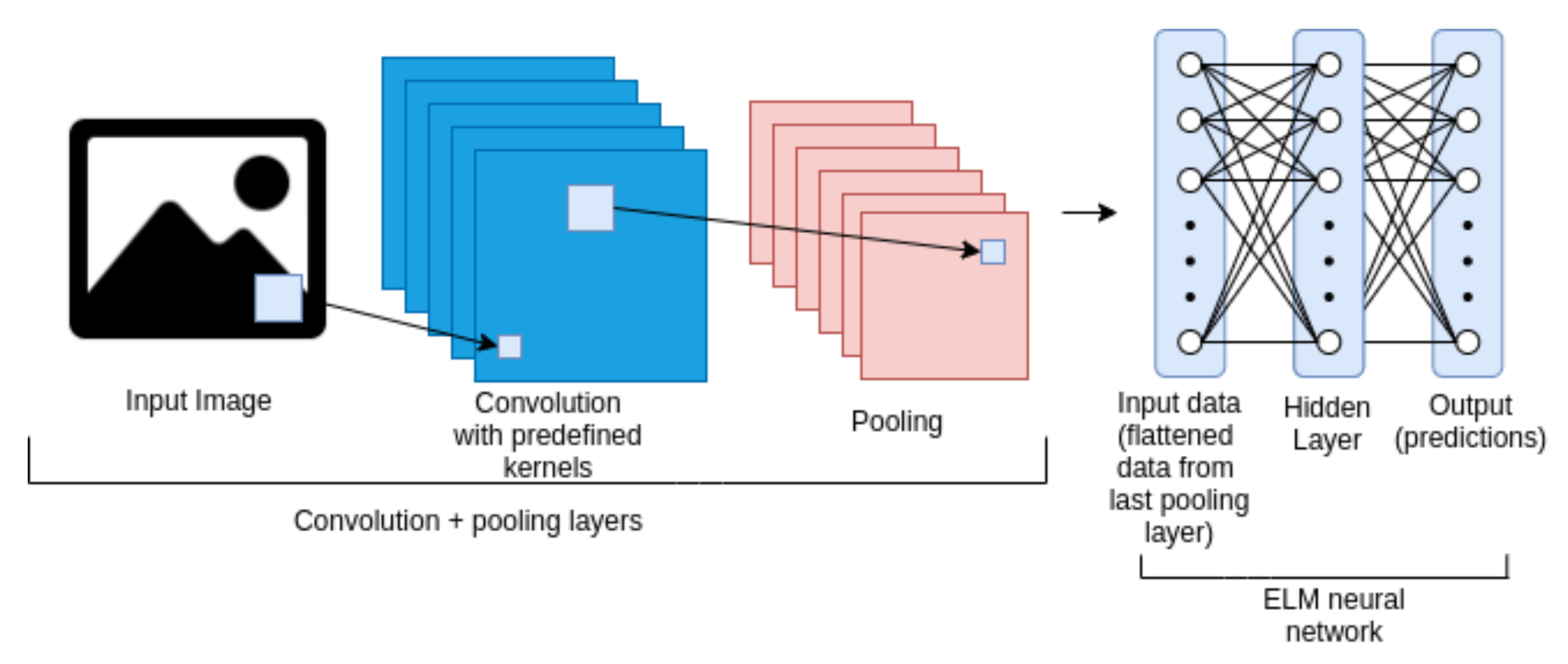
CNN-based approaches with predefined kernels for feature extraction provide good results in terms of accuracy and training time. In two scenarios (object and face recognition), the architectures of this type presented better accuracy [27,81] than other approaches, such as the deep belief network and stacked autoencoders. The excellent performance of this approach in the computational aspect is due to its one-way training style. The feature extraction is the most costly stage due to the high number of matrix operations in the CNN. However, when it comes to the training stage using ELM, the processing time is not an aggravating factor, except when the architectures’ complexity is increased.

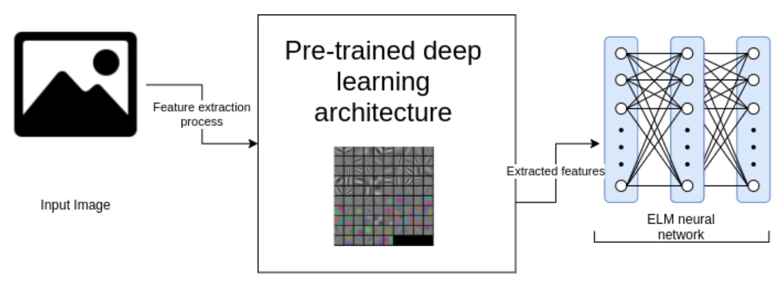
Regarding the approaches that use pre-trained CNN architectures (in the same or other domain) to extract characteristics and perform later fine-tuning with am ELM, it is also observed that the results are satisfactory. This approach outperforms others in the remote sensing and RGB-D image recognition scenarios [49,94] when considering the accuracy metric. Classic CNNs and support vector machines are examples of outperformed approaches. This approach’s training method is also a one-way training style, which explains the excellent training time involved in the learning process.

The fast training approaches for CNN models using ELM concepts could not be further analyzed, because only a few studies were found in the literature. However, one can note that this approach outperforms other CELM models, such as ELM-LRF and PCANet-ELM, in terms of accuracy when considering the handwritten digit recognition problem [30]. Instead of using the backpropagation algorithm for feature training, the authors used the ELM-AE network, obtaining a more compact representation of data and better training time.

In general, CELM presented interesting results regarding the accuracy as compared to several proposals that were found in the literature. Despite not having the same power as the conventional CNNs (with fully connected layers and backpropagation) to extract features, the CELM’s accuracy proved competitive in the analyzed scenarios and benchmark datasets. The competitiveness of the results is clear when, in many cases, CELM was superior to several traditional models, such as MLP (as in [50,69,102]) and SVM (as in [46,90,113]). Observing these results, we reported a good generalization and good representativeness for the CELM [27,49,55,57,68,97,104].

From the primary studies, we also notice that CELM architectures have good convergence and provide better accuracy. Changing the fully connected layers to an ELM network consequently increases the training speed and avoids fine adjustments [30,115,122,131]. Convergence is achieved without iterations and intensive updating of the network parameters. In the case of a CNN for feature extraction with an ELM, the training is done with the ELM after the extraction of CNN features. Rapid training reflects directly on computational performance. With the adoption of the CELM, it is possible to decrease the processing time that is required for the learning process. This feature makes the CELM able to solve problems on a large scale, such as real-time or big data applications [29,94,111].

7. Open Challenges

Despite the many advantages of the CELM architectures, such as suitable training time, test time, and accuracy, some open challenges can serve as inspiration for future research contributing to the advancement in the field of research into the CELM.

It is known that the number of layers can be an important factor in the ability to generalize a neural network. Classic studies of deep learning proposed architectures with multiple convolution layers [18,19,129]. However, when the number of layers is increased, problems with increasing training time and a loss of generalization capacity emerge [77], which can cause overfitting issues. These two reasons may explain the reason that many CELM architectures with predefined kernels do not use very complex architectures to extract features.

Despite the good performance of GPUs, sometimes it is not possible to use them in a real environment. When this happens, all of the data are stored sequentially in the RAM and processed by the CPU, increasing the training time, especially when handling data with high dimensionality. One possible way to overcome this issue is using approaches that aim at high-performance computing using parallel computing. Furthermore, the usage of strategies for batching the features can replace the number of samples N in the memory requirements [9]. There is an approach in the literature that aims to use an ELM for large-scale data problems, known as the high-performance extreme learning machine [9], which could be adequately analyzed in the context of the CELM.

Regarding the problem of the number of convolutional layers, the gradual increase in the complexity of the network can cause problems in the model generalization. This can decrease the accuracy and cause overfitting. Some studies in the literature have proposed using new structures that increase the number of layers without a loss in the generalization of the network and improve the accuracy results, such as residual blocks [19] and dense blocks [129]. This is another research challenge that can be considered in CELM architectures, increasing the number of layers to increase the accuracy without losing the network’s generalization capacity. These deep convolutional approaches should inspire CNN architectures for the CELM.

There is also a research field that aims to make deep learning models more compact, which would accelerate the learning process. Traditional CNN models generally demand high computational cost and, by compressing these models, it is possible to make them lighter in terms of their computational cost. Two well-known techniques used for CNN compression are pruning and weight quantization. The pruning process handles the removal of a subset of parameters (filters, layers, or weights) evaluated as less critical for the task. None of the studies reported in this systematic review reported the use of pruning or weight quantization. Approaches for pruning or weight quantization (or a combination of both) could improve the learning process of CELMs, removing irrelevant information in the neural network and optimizing the support for real-time applications.

In this systematic review, we did not report any work on object detection problems. Deep learning research field architectures for object detection, such as R-CNN, Mask R-CNN, and YOLO, could inspire new CELM studies. Such architectures have high computational costs. When the object detection deep learning models are processed into the CPU, there is a loss in computational performance. Developing new architectures for object detection using ELM concepts could help such applications where computational resources are limited.

Another common computer vision problem that recurs in the literature and it is little addressed in this systematic review is semantic segmentation. The difficulty may be linked to image reconstruction and decoding operations through deconvolutions usually done through the backpropagation algorithm. This is another open challenge in the CELM, where ELM networks could replace the backpropagation in the calculation to update the weights of both convolutional and deconvolutional layers for the reconstruction of the segmented images.

Despite presenting promising and interesting results in RGB-D classification and remote sensing tasks, there is a lack of CELM networks in this area. There are no studies to date that prove the strength of the CELM in very large datasets for even more complex tasks. Therefore, there is a need for a performance evaluation (accuracy and computation) of CELM models on the large current state of the art, such as ImageNet, the COCO dataset, and Pascal-VOC. These last three cited databases are current references in deep learning for image classification, object detection, and semantic segmentation, in addition to other problems, such as the detection of human poses and panoptic segmentation, and so on. The performing of new experiments on the state of the art datasets in deep learning can strengthen all aspects of the CELM’s advantages that are covered in this systematic review.

8. Conclusions

CELMs are quick-training CNNs that avoid the use of backpropagation calculations for updating the network weights. Filters are efficiently defined for the feature extraction step, and least-squares obtain weights in the classification stage’s output layer through an ELM network.

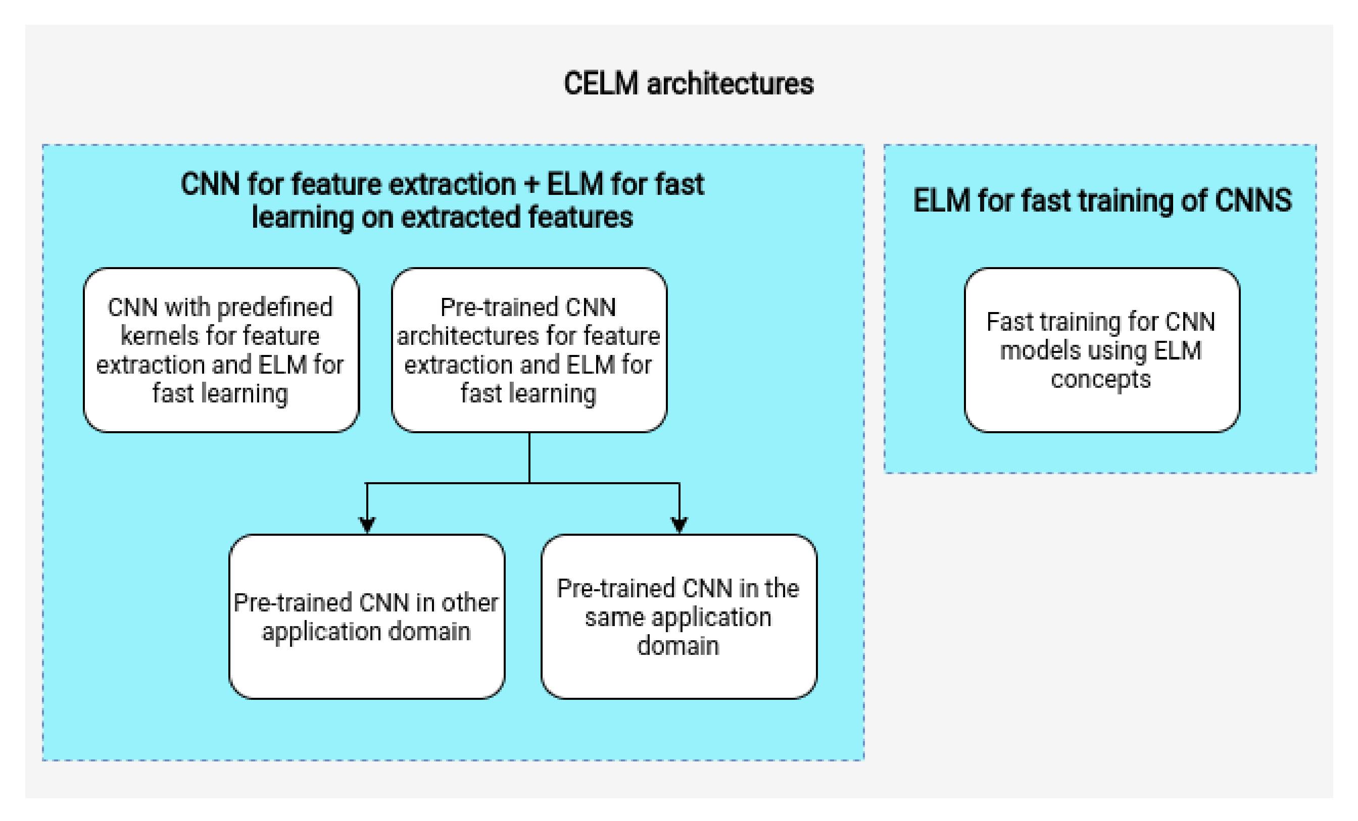
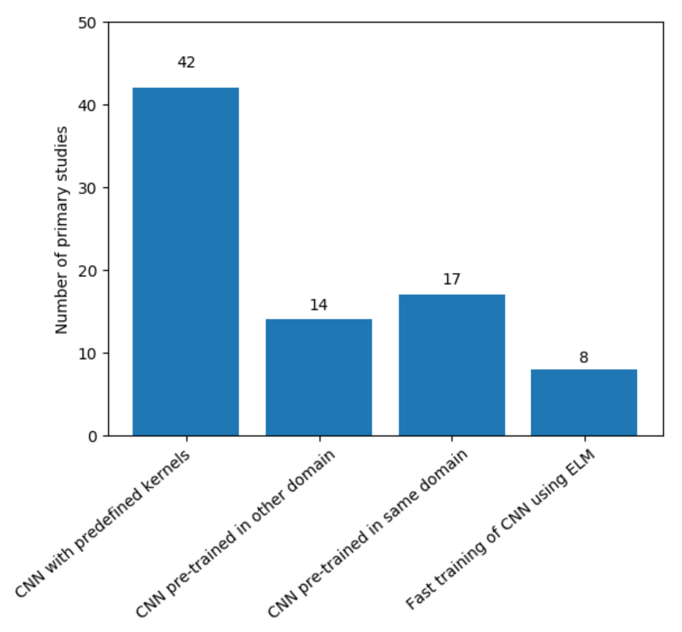
We presented a systematic review on the CELM in image analysis while considering the literature published over the last 10 years. Initially, we collected 2220 articles, and after removing duplicate and applying inclusion criteria, we analyzed 81 studies on the CELM. We reported 19 different scenarios, and object recognition was the most common application where the CELM was used. Additionally, we have found and classified the studies into four different types of CELM architectures: (i) a CNN with predefined kernels for feature extraction and an ELM for fast training; (ii) a pre-trained CNN in other application domains for feature extraction and an ELM for fast training; (iii) a pre-trained CNN in the same application domain for feature extraction and an ELM for fast training; and, (iv) the fast training of CNNs using ELM concepts. The CNN with predefined kernels was the most common architecture that was proposed in the literature, followed by the pre-trained CNN in same application domain.

Analyzing the primary studies, we can state that CELM models provide good accuracy and good computational performance. We highlight the excellent feature representation that is achieved by the CELM, which can explain its good accuracy results. In general, the CELM architectures present fast convergence by changing the conventional fully connected layers to the ELM network. This change avoids fine adjustments by the backpropagation algorithm’s iterations. Finally, there is a decrease in the total processing time that is required for the learning process when using CELM architectures, making it suitable to solve image analysis problems in real-time applications.

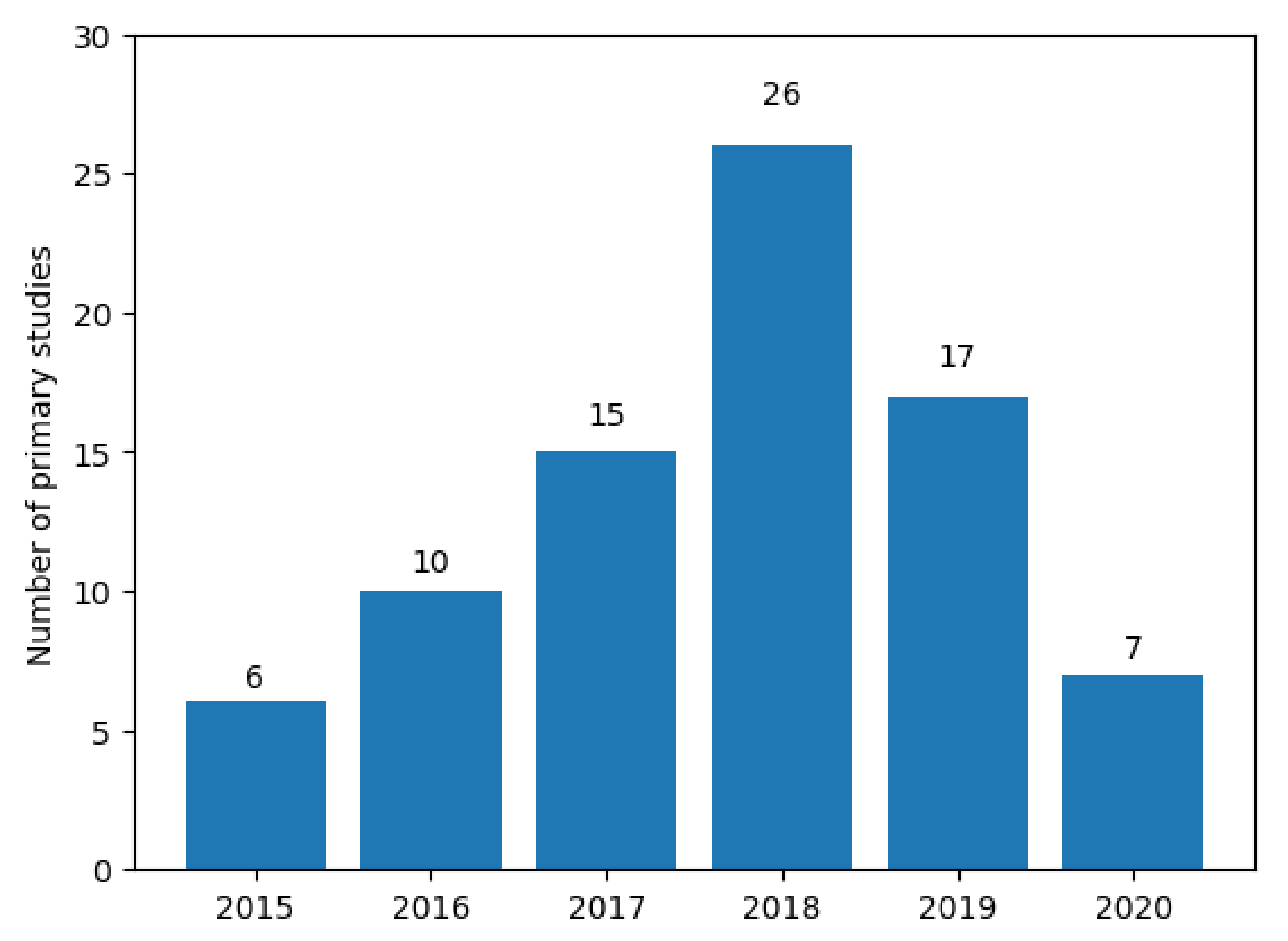
As limitations of this work, we could initially cite the range of the systematic review; it was focused on the last 10 years of the literature, but, as presented, the first papers regarding the CELM were published in 2015, and most of them after 2018. Moreover, as time passes and the CELM becomes a more active research area, other new studies are constantly being published, and keeping the systematic review up-to-date is a difficult task.

In terms of future research that is based on the findings and open challenges of this systematic review, we highlight the following directions: (i) strategies to increase the number of convolutional layers without negative impacts on overfitting, training time, and generalization issues; (ii) optimized implementations of the ELM for high-performance computing in the context of the CELM can address the training time issue; (iii) pruning, compaction, and/or quantization techniques for convolution layers may accelerate the learning process; (iv) the implementation of new CELM architectures inspired by traditional deep learning architectures—e.g., R-CNN, Mask R-CNN, and YOLO—for object detection and image segmentation; and, (v) regarding the reconstruction of segmented images, it would be possible to investigate the use of ELM networks to replace backpropagation in the calculation of the updates of the weights of the deconvolutional/upsampling layers.

References

1. LeCun, Y.; Bengio, Y.; Hinton, G. Deep learning. Nature 2015, 521, 436–444. [Google Scholar] [CrossRef] [PubMed]
2. Rawat, W.; Wang, Z. Deep convolutional neural networks for image classification: A comprehensive review. Neural Comput. 2017, 29, 2352–2449. [Google Scholar] [CrossRef] [PubMed]
3. Redmon, J.; Divvala, S.; Girshick, R.; Farhadi, A. You only look once: Unified, real-time object detection. In Proceedings of the IEEE Conference on Computer Vision and Pattern Recognition, Las Vegas, NV, USA, 27–30 June 2016; pp. 779–788. [Google Scholar]
4. Guo, Y.; Liu, Y.; Georgiou, T.; Lew, M.S. A review of semantic segmentation using deep neural networks. Int. J. Multimed. Inf. Retr. 2018, 7, 87–93. [Google Scholar] [CrossRef] [Green Version]
5. Shen, D.; Wu, G.; Suk, H.I. Deep learning in medical image analysis. Annu. Rev. Biomed. Eng. 2017, 19, 221–248. [Google Scholar] [CrossRef] [PubMed] [Green Version]
6. Huang, G.; Bai, Z.; Kasun, L.L.C.; Vong, C.M. Local Receptive Fields Based Extreme Learning Machine. IEEE Comput. Intell. Mag. 2015, 10, 18–29. [Google Scholar] [CrossRef]
7. Huang, G.B.; Zhu, Q.Y.; Siew, C.K. Extreme learning machine: Theory and applications. Neurocomputing 2006, 70, 489–501. [Google Scholar] [CrossRef]
8. Cao, J.; Lin, Z. Extreme learning machines on high dimensional and large data applications: A survey. Math. Probl. Eng. 2015, 2015, 103796. [Google Scholar] [CrossRef]
9. Akusok, A.; Björk, K.M.; Miche, Y.; Lendasse, A. High-performance extreme learning machines: A complete toolbox for big data applications. IEEE Access 2015, 3, 1011–1025. [Google Scholar] [CrossRef]
10. dos Santos, M.M.; da Silva Filho, A.G.; dos Santos, W.P. Deep convolutional extreme learning machines: Filters combination and error model validation. Neurocomputing 2019, 329, 359–369. [Google Scholar] [CrossRef]
11. Huang, G.B.; Wang, D.H.; Lan, Y. Extreme learning machines: A survey. Int. J. Mach. Learn. Cybern. 2011, 2, 107–122. [Google Scholar] [CrossRef]
12. Huang, G.; Huang, G.B.; Song, S.; You, K. Trends in extreme learning machines: A review. Neural Networks 2015, 61, 32–48. [Google Scholar] [CrossRef]
13. Salaken, S.M.; Khosravi, A.; Nguyen, T.; Nahavandi, S. Extreme learning machine based transfer learning algorithms: A survey. Neurocomputing 2017, 267, 516–524. [Google Scholar] [CrossRef]
14. Zhang, J.; Li, Y.; Xiao, W.; Zhang, Z. Non-iterative and Fast Deep Learning: Multilayer Extreme Learning Machines. J. Frankl. Inst. 2020, 357, 8925–8955. [Google Scholar] [CrossRef]
15. Endo, P.T.; Rodrigues, M.; Gonçalves, G.E.; Kelner, J.; Sadok, D.H.; Curescu, C. High availability in clouds: Systematic review and research challenges. J. Cloud Comput. 2016, 5, 16. [Google Scholar] [CrossRef] [Green Version]
16. Coutinho, E.F.; de Carvalho Sousa, F.R.; Rego, P.A.L.; Gomes, D.G.; de Souza, J.N. Elasticity in cloud computing: A survey. Ann. Telecommun.-Ann. Télécommun. 2015, 70, 289–309. [Google Scholar] [CrossRef]
17. Kitchenham, B. Procedures for performing systematic reviews. Keele, UK Keele Univ. 2004, 33, 1–26. [Google Scholar]
18. Simonyan, K.; Zisserman, A. Very Deep Convolutional Networks for Large-Scale Image Recognition. In Proceedings of the 3rd International Conference on Learning Representations, ICLR 2015, San Diego, CA, USA, 7–9 May 2015. [Google Scholar]
19. He, K.; Zhang, X.; Ren, S.; Sun, J. Deep residual learning for image recognition. In Proceedings of the IEEE Conference on Computer Vision and Pattern Recognition, Las Vegas, NV, USA, 27–30 June 2016; pp. 770–778. [Google Scholar]
20. Ioffe, S.; Szegedy, C. Batch Normalization: Accelerating Deep Network Training by Reducing Internal Covariate Shift. In Proceedings of the International Conference on Machine Learning (ICML), Lille, France, 6–11 July 2015. [Google Scholar]
21. Srivastava, N.; Hinton, G.; Krizhevsky, A.; Sutskever, I.; Salakhutdinov, R. Dropout: A simple way to prevent neural networks from overfitting. J. Mach. Learn. Res. 2014, 15, 1929–1958. [Google Scholar]
22. Gu, J.; Wang, Z.; Kuen, J.; Ma, L.; Shahroudy, A.; Shuai, B.; Liu, T.; Wang, X.; Wang, G.; Cai, J.; et al. Recent advances in convolutional neural networks. Pattern Recognit. 2018, 77, 354–377. [Google Scholar] [CrossRef] [Green Version]
23. Xu, X.; Li, G.; Xie, G.; Ren, J.; Xie, X. Weakly supervised deep semantic segmentation using CNN and ELM with semantic candidate regions. Complexity 2019, 2019, 9180391. [Google Scholar] [CrossRef]
24. Yoo, Y.; Oh, S.Y. Fast training of convolutional neural network classifiers through extreme learning machines. In Proceedings of the 2016 International Joint Conference on Neural Networks (IJCNN), Vancouver, BC, Canada, 24–29 July 2016; pp. 1702–1708. [Google Scholar]
25. Bai, Z.; Kasun, L.; Huang, G.B. Generic Object Recognition with Local Receptive Fields Based Extreme Learning Machine. Procedia Comput. Sci. 2015, 53, 391–399. [Google Scholar] [CrossRef] [Green Version]
26. He, B.; Song, Y.; Zhu, Y.; Sha, Q.; Shen, Y.; Yan, T.; Nian, R.; Lendasse, A. Local receptive fields based extreme learning machine with hybrid filter kernels for image classification. Multidimens. Syst. Signal Process. 2019, 30, 1149–1169. [Google Scholar] [CrossRef]
27. Wu, C.; Li, Y.; Zhao, Z.; Liu, B. Extreme learning machine with autoencoding receptive fields for image classification. Neural Comput. Appl. 2020, 32, 8157–8173. [Google Scholar] [CrossRef]
28. Wu, C.; Li, Y.; Zhao, Z.; Liu, B. Extreme learning machine with multi-structure and auto encoding receptive fields for image classification. Multidimens. Syst. Signal Process. 2020, 31, 1277–1298. [Google Scholar] [CrossRef]
29. Song, G.; Dai, Q.; Han, X.; Guo, L. Two novel ELM-based stacking deep models focused on image recognition. Appl. Intell. 2020, 50, 1345–1366. [Google Scholar] [CrossRef]
30. Chang, P.; Zhang, J.; Wang, J.; Fei, R. ELMAENet: A Simple, Effective and Fast Deep Architecture for Image Classification. Neural Process. Lett. 2020, 51, 129–146. [Google Scholar] [CrossRef]
31. Alshalali, T.; Josyula, D. Fine-Tuning of Pre-Trained Deep Learning Models with Extreme Learning Machine. In Proceedings of the 2018 International Conference on Computational Science and Computational Intelligence (CSCI), Las Vegas, NV, USA, 12–14 December 2018; pp. 469–473. [Google Scholar]
32. Han, J.S.; Cho, G.B.; Kwak, K.C. A Design of Convolutional Neural Network Using ReLU-Based ELM Classifier and Its Application. In Proceedings of the 9th International Conference on Machine Learning and Computing, Singapore, 24–26 February 2017; pp. 179–183. [Google Scholar]
33. Hao, P.; Zhai, J.H.; Zhang, S.F. A simple and effective method for image classification. In Proceedings of the 2017 International Conference on Machine Learning and Cybernetics (ICMLC), Ningbo, China, 9–12 July 2017; Volume 1, pp. 230–235. [Google Scholar]
34. Cui, D.; Zhang, G.; Han, W.; Lekamalage Chamara Kasun, L.; Hu, K.; Huang, G.B. Compact feature representation for image classification using elms. In Proceedings of the IEEE International Conference on Computer Vision Workshops, Venice, Italy, 22–29 October 2017; pp. 1015–1022. [Google Scholar]
35. Zhu, X.; Li, Z.; Zhang, X.Y.; Li, P.; Xue, Z.; Wang, L. Deep convolutional representations and kernel extreme learning machines for image classification. Multimed. Tools Appl. 2019, 78, 29271–29290. [Google Scholar] [CrossRef]
36. Zhang, L.; He, Z.; Liu, Y. Deep object recognition across domains based on adaptive extreme learning machine. Neurocomputing 2017, 239, 194–203. [Google Scholar] [CrossRef]
37. Zhang, L.; Zhang, D.; Tian, F. SVM and ELM: Who Wins? Object recognition with deep convolutional features from ImageNet. In Proceedings of ELM-2015; Springer: Berlin, Germany, 2016; Volume 1, pp. 249–263. [Google Scholar]
38. Liu, H.; Li, F.; Xu, X.; Sun, F. Active object recognition using hierarchical local-receptive-field-based extreme learning machine. Memetic Comput. 2018, 10, 233–241. [Google Scholar] [CrossRef]
39. He, X.; Liu, H.; Huang, W. Room categorization using local receptive fields-based extreme learning machine. In Proceedings of the 2017 2nd International Conference on Advanced Robotics and Mechatronics (ICARM), Hefei and Tai’an, China, 27–31 August 2017; pp. 620–625. [Google Scholar]
40. LeCun, Y.; Huang, F.J.; Bottou, L. Learning methods for generic object recognition with invariance to pose and lighting. In Proceedings of the 2004 IEEE Computer Society Conference on Computer Vision and Pattern Recognition, CVPR 2004, Washington, DC, USA, 27 June–2 July 2004; Volume 2, pp. II–104. [Google Scholar]
41. Krizhevsky, A.; Hinton, G. Learning Multiple Layers of Features From Tiny Images. 2009. Available online: http://citeseerx.ist.psu.edu/viewdoc/download?doi=10.1.1.222.9220&rep=rep1&type=pdf (accessed on 8 April 2009).
42. Nene, S.A.; Nayar, S.K.; Murase, H. Columbia Object Image Library (Coil-100); Columbia University: New York, NY, USA, 1996. [Google Scholar]
43. Fei-Fei, L.; Fergus, R.; Perona, P. Learning generative visual models from few training examples: An incremental bayesian approach tested on 101 object categories. In Proceedings of the 2004 Conference on Computer Vision and Pattern Recognition Workshop, Washington, DC, USA, 27 June–2 July 2004; p. 178. [Google Scholar]
44. Leibe, B.; Schiele, B. Analyzing appearance and contour based methods for object categorization. In Proceedings of the 2003 IEEE Computer Society Conference on Computer Vision and Pattern Recognition, Madison, WI, USA, 18–20 June 2003; Volume 2, pp. II–409. [Google Scholar]
45. Ma, L.; Liu, Y.; Zhang, X.; Ye, Y.; Yin, G.; Johnson, B.A. Deep learning in remote sensing applications: A meta-analysis and review. ISPRS J. Photogramm. Remote Sens. 2019, 152, 166–177. [Google Scholar] [CrossRef]
46. Huang, F.; Lu, J.; Tao, J.; Li, L.; Tan, X.; Liu, P. Research on Optimization Methods of ELM Classification Algorithm for Hyperspectral Remote Sensing Images. IEEE Access 2019, 7, 108070–108089. [Google Scholar] [CrossRef]
47. Shen, Y.; Xiao, L.; Chen, J.; Pan, D. A Spectral-Spatial Domain-Specific Convolutional Deep Extreme Learning Machine for Supervised Hyperspectral Image Classification. IEEE Access 2019, 7, 132240–132252. [Google Scholar] [CrossRef]
48. Shi, J.; Ku, J. Spectral-spatial classification of hyperspectral image using distributed extreme learning machine with MapReduce. In Proceedings of the 2017 IEEE 2nd International Conference on Big Data Analysis (ICBDA), Beijing, China, 10–12 March 2017; pp. 714–720. [Google Scholar]
49. Cao, F.; Yang, Z.; Ren, J.; Ling, B.W.K. Convolutional neural network extreme learning machine for effective classification of hyperspectral images. J. Appl. Remote Sens. 2018, 12, 035003. [Google Scholar] [CrossRef]
50. Li, J.; Zhao, X.; Li, Y.; Du, Q.; Xi, B.; Hu, J. Classification of hyperspectral imagery using a new fully convolutional neural network. IEEE Geosci. Remote Sens. Lett. 2018, 15, 292–296. [Google Scholar] [CrossRef]
51. Lv, Q.; Niu, X.; Dou, Y.; Xu, J.; Lei, Y. Classification of hyperspectral remote sensing image using hierarchical local-receptive-field-based extreme learning machine. IEEE Geosci. Remote Sens. Lett. 2016, 13, 434–438. [Google Scholar] [CrossRef]
52. Lv, Q.; Niu, X.; Dou, Y.; Wang, Y.; Xu, J.; Zhou, J. Hyperspectral image classification via kernel extreme learning machine using local receptive fields. In Proceedings of the 2016 IEEE International Conference on Image Processing (ICIP), Phoenix, AZ, USA, 25–28 September 2016; pp. 256–260. [Google Scholar]
53. Lv, Q.; Niu, X.; Dou, Y.; Xu, J.; Xia, F. Leveraging local receptive fields based random weights networks for hyperspectral image classification. J. Intell. Fuzzy Syst. 2016, 31, 1017–1028. [Google Scholar] [CrossRef]
54. Shen, Y.; Chen, J.; Xiao, L. Supervised classification of hyperspectral images using local-receptive-fields-based kernel extreme learning machine. In Proceedings of the 2017 IEEE International Conference on Image Processing (ICIP), Beijing, China, 17–20 September 2017; pp. 3120–3124. [Google Scholar]
55. Gu, Y.; Xu, Y.; Liu, J. SAR ATR by Decision Fusion of Multiple Random Convolution Features. In Proceedings of the 2019 22th International Conference on Information Fusion (FUSION), Ottawa, ON, Canada, 2–5 July 2019; pp. 1–8. [Google Scholar]
56. Wang, P.; Zhang, X.; Hao, Y. A Method Combining CNN and ELM for Feature Extraction and Classification of SAR Image. J. Sens. 2019, 2019. [Google Scholar] [CrossRef]
57. Ye, L.; Wang, L.; Sun, Y.; Zhu, R.; Wei, Y. Aerial scene classification via an ensemble extreme learning machine classifier based on discriminative hybrid convolutional neural networks features. Int. J. Remote Sens. 2019, 40, 2759–2783. [Google Scholar] [CrossRef]
58. Romay, D.M.G. Hyperspectral Remote Sensing Scenes; Universidad del País Vasco (UPV/EHU): Leioa, Spain, 2020. [Google Scholar]
59. Keydel, E.R.; Lee, S.W.; Moore, J.T. MSTAR extended operating conditions: A tutorial. In Algorithms for Synthetic Aperture Radar Imagery III; International Society for Optics and Photonics: Orlando, FL, USA, 1996; Volume 2757, pp. 228–242. [Google Scholar]
60. Coman, C. A deep learning sar target classification experiment on mstar dataset. In Proceedings of the 2018 19th International Radar Symposium (IRS), Bonn, Germany, 20–22 June 2018; pp. 1–6. [Google Scholar]
61. Özyurt, F.; Sert, E.; Avcı, D. An expert system for brain tumor detection: Fuzzy C-means with super resolution and convolutional neural network with extreme learning machine. Med Hypotheses 2020, 134, 109433. [Google Scholar] [CrossRef]
62. Pashaei, A.; Sajedi, H.; Jazayeri, N. Brain tumor classification via convolutional neural network and extreme learning machines. In Proceedings of the 2018 8th International Conference on Computer and Knowledge Engineering (ICCKE), Mashhad, Iran, 25–26 October 2018; pp. 314–319. [Google Scholar]
63. Ari, A.; Hanbay, D. Deep learning based brain tumor classification and detection system. TUrkish J. Electr. Eng. Comput. Sci. 2018, 26, 2275–2286. [Google Scholar] [CrossRef]
64. Yu, J.S.; Chen, J.; Xiang, Z.; Zou, Y.X. A hybrid convolutional neural networks with extreme learning machine for WCE image classification. In Proceedings of the 2015 IEEE International Conference on Robotics and Biomimetics (ROBIO), Zhuhai, China, 6–9 December 2015; pp. 1822–1827. [Google Scholar]
65. Doğantekin, A.; Özyurt, F.; Avcı, E.; Koç, M. A novel approach for liver image classification: PH-C-ELM. Measurement 2019, 137, 332–338. [Google Scholar] [CrossRef]
66. Özyurt, F. A fused CNN model for WBC detection with MRMR feature selection and extreme learning machine. Soft Comput. 2020, 24, 8163–8172. [Google Scholar] [CrossRef]
67. Fang, J.; Xu, X.; Liu, H.; Sun, F. Local receptive field based extreme learning machine with three channels for histopathological image classification. Int. J. Mach. Learn. Cybern. 2019, 10, 1437–1447. [Google Scholar] [CrossRef]
68. Lu, S.; Xia, K.; Wang, S.H. Diagnosis of cerebral microbleed via VGG and extreme learning machine trained by Gaussian map bat algorithm. J. Ambient. Intell. Humaniz. Comput. 2020, 1–12. [Google Scholar] [CrossRef] [Green Version]
69. Ghoneim, A.; Muhammad, G.; Hossain, M.S. Cervical cancer classification using convolutional neural networks and extreme learning machines. Future Gener. Comput. Syst. 2020, 102, 643–649. [Google Scholar] [CrossRef]
70. Monkam, P.; Qi, S.; Xu, M.; Li, H.; Han, F.; Teng, Y.; Qian, W. Ensemble learning of multiple-view 3D-CNNs model for micro-nodules identification in CT images. IEEE Access 2018, 7, 5564–5576. [Google Scholar] [CrossRef]
71. Fang, L.; Wang, C.; Li, S.; Yan, J.; Chen, X.; Rabbani, H. Automatic classification of retinal three-dimensional optical coherence tomography images using principal component analysis network with composite kernels. J. Biomed. Opt. 2017, 22, 116011. [Google Scholar] [CrossRef]
72. Li, S.; Jiang, H.; Pang, W. Joint multiple fully connected convolutional neural network with extreme learning machine for hepatocellular carcinoma nuclei grading. Comput. Biol. Med. 2017, 84, 156–167. [Google Scholar] [CrossRef]
73. Baldominos, A.; Saez, Y.; Isasi, P. A survey of handwritten character recognition with mnist and emnist. Appl. Sci. 2019, 9, 3169. [Google Scholar] [CrossRef] [Green Version]
74. Khellal, A.; Ma, H.; Fei, Q. Convolutional Neural Network Features Comparison Between Back-Propagation and Extreme Learning Machine. In Proceedings of the 2018 37th Chinese Control Conference (CCC), Wuhan, China, 25–27 July 2018; pp. 9629–9634. [Google Scholar]
75. Kannojia, S.P.; Jaiswal, G. Ensemble of hybrid CNN-ELM model for image classification. In Proceedings of the 2018 5th International Conference on Signal Processing and Integrated Networks (SPIN), Noida, India, 22–23 February 2018; pp. 538–541. [Google Scholar]
76. Ding, S.; Guo, L.; Hou, Y. Extreme learning machine with kernel model based on deep learning. Neural Comput. Appl. 2017, 28, 1975–1984. [Google Scholar] [CrossRef]
77. Pang, S.; Yang, X. Deep convolutional extreme learning machine and its application in handwritten digit classification. Comput. Intell. Neurosci. 2016, 2016. [Google Scholar] [CrossRef] [PubMed] [Green Version]
78. LeCun, Y.; Cortes, C.; Burges, C. THE MNIST DATABASE: Of Handwritten Digits. 1998. Available online: http://yann.lecun.com/exdb/mnist/ (accessed on 25 August 2020).
79. Hull, J.J. A database for handwritten text recognition research. IEEE Trans. Pattern Anal. Mach. Intell. 1994, 16, 550–554. [Google Scholar] [CrossRef]
80. Hu, G.; Yang, Y.; Yi, D.; Kittler, J.; Christmas, W.; Li, S.Z.; Hospedales, T. When face recognition meets with deep learning: An evaluation of convolutional neural networks for face recognition. In Proceedings of the IEEE International Conference on Computer Vision Workshops, Santiago, Chile, 7–13 December 2015; pp. 142–150. [Google Scholar]
81. Yu, D.; Wu, X.J. 2DPCANet: A deep leaning network for face recognition. Multimed. Tools Appl. 2018, 77, 12919–12934. [Google Scholar] [CrossRef]
82. Ripon, K.S.N.; Ali, L.E.; Siddique, N.; Ma, J. Convolutional Neural Network based Eye Recognition from Distantly Acquired Face Images for Human Identification. In Proceedings of the 2019 International Joint Conference on Neural Networks (IJCNN), Budapest, Hungary, 14–19 July 2019; pp. 1–8. [Google Scholar]
83. Wang, K.; Liu, M.; Hao, X.; Xing, X. Decision-Level Fusion Method Based on Deep Learning. In Proceedings of the Chinese Conference on Biometric Recognition, Shenzhen, China, 28–29 October 2017; Springer: Cham, Switzerland, 2017; pp. 673–682. [Google Scholar]
84. Gürpınar, F.; Kaya, H.; Salah, A.A. Combining deep facial and ambient features for first impression estimation. In European Conference on Computer Vision; Springer: Cham, Switzerland, 2016; pp. 372–385. [Google Scholar]
85. Yale. The Normalized Yale Face Database. 1998. Available online: https://vismod.media.mit.edu/vismod/classes/mas622-00/datasets/ (accessed on 25 August 2020).
86. Hoyer, P.O. Non-negative matrix factorization with sparseness constraints. J. Mach. Learn. Res. 2004, 5, 1457–1469. [Google Scholar]
87. Cai, Z.; Han, J.; Liu, L.; Shao, L. RGB-D datasets using microsoft kinect or similar sensors: A survey. Multimed. Tools Appl. 2017, 76, 4313–4355. [Google Scholar] [CrossRef] [Green Version]
88. Wang, P.; Li, W.; Ogunbona, P.; Wan, J.; Escalera, S. RGB-D-based human motion recognition with deep learning: A survey. Comput. Vis. Image Underst. 2018, 171, 118–139. [Google Scholar] [CrossRef] [Green Version]
89. Shao, L.; Han, J.; Kohli, P.; Zhang, Z. Computer Vision and Machine Learning with RGB-D Sensors; Springer International Publishing: Basel, Switzerland, 2014; Volume 20. [Google Scholar]
90. Boubou, S.; Narikiyo, T.; Kawanishi, M. Object recognition from 3d depth data with extreme learning machine and local receptive field. In Proceedings of the 2017 IEEE International Conference on Advanced Intelligent Mechatronics (AIM), Munich, Germany, 3–7 July 2017; pp. 394–399. [Google Scholar]
91. Liu, H.; Li, F.; Xu, X.; Sun, F. Multi-modal local receptive field extreme learning machine for object recognition. Neurocomputing 2018, 277, 4–11. [Google Scholar] [CrossRef]
92. Yin, Y.; Li, H. Multi-view CSPMPR-ELM feature learning and classifying for RGB-D object recognition. Clust. Comput. 2019, 22, 8181–8191. [Google Scholar] [CrossRef]
93. Yin, Y.; Li, H. RGB-D object recognition based on the joint deep random kernel convolution and ELM. J. Ambient. Intell. Humaniz. Comput. 2018, 11, 4337–4346. [Google Scholar] [CrossRef]
94. Zaki, H.F.; Shafait, F.; Mian, A. Viewpoint invariant semantic object and scene categorization with RGB-D sensors. Auton. Robot. 2019, 43, 1005–1022. [Google Scholar] [CrossRef]
95. Yin, Y.; Li, H.; Wen, X. Multi-model convolutional extreme learning machine with kernel for RGB-D object recognition. In LIDAR Imaging Detection and Target Recognition 2017; International Society for Optics and Photonics: Changchun, China, 2017; Volume 10605, p. 106051Z. [Google Scholar]
96. Yang, Z.X.; Tang, L.; Zhang, K.; Wong, P.K. Multi-view cnn feature aggregation with elm auto-encoder for 3d shape recognition. Cogn. Comput. 2018, 10, 908–921. [Google Scholar] [CrossRef]
97. Ijjina, E.P.; Chalavadi, K.M. Human action recognition in RGB-D videos using motion sequence information and deep learning. Pattern Recognit. 2017, 72, 504–516. [Google Scholar] [CrossRef]
98. Lai, K.; Bo, L.; Ren, X.; Fox, D. A large-scale hierarchical multi-view rgb-d object dataset. In Proceedings of the 2011 IEEE International Conference on Robotics and Automation, Shanghai, China, 9–13 May 2011; pp. 1817–1824. [Google Scholar]
99. Martinel, N.; Piciarelli, C.; Foresti, G.L.; Micheloni, C. Mobile food recognition with an extreme deep tree. In Proceedings of the 10th International Conference on Distributed Smart Camera, Paris, France, 12–15 September 2016; pp. 56–61. [Google Scholar]
100. Li, Z.; Zhu, X.; Wang, L.; Guo, P. Image classification using convolutional neural networks and kernel extreme learning machines. In Proceedings of the 2018 25th IEEE International Conference on Image Processing (ICIP), Athens, Greece, 7–10 October 2018; pp. 3009–3013. [Google Scholar]
101. Horii, K.; Maeda, K.; Ogawa, T.; Haseyama, M. A Human-Centered Neural Network Model with Discriminative Locality Preserving Canonical Correlation Analysis for Image Classification. In Proceedings of the 2018 25th IEEE International Conference on Image Processing (ICIP), Athens, Greece, 7–10 October 2018; pp. 2366–2370. [Google Scholar]
102. Pashaei, A.; Ghatee, M.; Sajedi, H. Convolution neural network joint with mixture of extreme learning machines for feature extraction and classification of accident images. J. Real-Time Image Process. 2020, 17, 1051–1066. [Google Scholar] [CrossRef]
103. Zeng, Y.; Xu, X.; Fang, Y.; Zhao, K. Traffic sign recognition using deep convolutional networks and extreme learning machine. In Proceedings of the International Conference on Intelligent Science and Big Data Engineering, Cham, Switzerland, 22 October 2015; Springer: Cham, Switzerland, 2015; pp. 272–280. [Google Scholar]
104. Zhou, Y.; Liu, Q.; Zhao, Y.; Li, W. Aluminum Foil Packaging Sealing Testing Method Based on Gabor Wavelet and ELM Neural Network. In Proceedings of the 2nd International Conference on Advances in Image Processing, Chengdu, China, 16–18 June 2018; pp. 59–63. [Google Scholar]
105. Liu, H.; Fang, J.; Xu, X.; Sun, F. Surface material recognition using active multi-modal extreme learning machine. Cogn. Comput. 2018, 10, 937–950. [Google Scholar] [CrossRef]
106. Xu, X.; Fang, J.; Li, Q.; Xie, G.; Xie, J.; Ren, M. Multi-scale local receptive field based online sequential extreme learning machine for material classification. In Proceedings of the International Conference on Cognitive Systems and Signal Processing, Singapore, 28 April 2018; Springer: Singapore, 2018; pp. 37–53. [Google Scholar]
107. Zhang, Y.; Zhang, L.; Li, P. A novel biologically inspired ELM-based network for image recognition. Neurocomputing 2016, 174, 286–298. [Google Scholar] [CrossRef]
108. Imran, J.; Raman, B. Deep motion templates and extreme learning machine for sign language recognition. Vis. Comput. 2020, 36, 1233–1246. [Google Scholar] [CrossRef]
109. Xie, X.; Guo, W.; Jiang, T. Body Gestures Recognition Based on CNN-ELM Using Wi-Fi Long Preamble. In Proceedings of the International Conference in Communications, Signal Processing, and Systems, Singapore, 14 August 2018; Springer: Singapore, 2018; pp. 877–889. [Google Scholar]
110. Sun, R.; Wang, X.; Yan, X. Robust visual tracking based on convolutional neural network with extreme learning machine. Multimed. Tools Appl. 2019, 78, 7543–7562. [Google Scholar] [CrossRef]
111. Huang, J.; Yu, Z.L.; Cai, Z.; Gu, Z.; Cai, Z.; Gao, W.; Yu, S.; Du, Q. Extreme learning machine with multi-scale local receptive fields for texture classification. Multidimens. Syst. Signal Process. 2017, 28, 995–1011. [Google Scholar] [CrossRef]
112. Kölsch, A.; Afzal, M.Z.; Ebbecke, M.; Liwicki, M. Real-time document image classification using deep CNN and extreme learning machines. In Proceedings of the 14th IAPR International Conference on Document Analysis and Recognition (ICDAR), Kyoto, Japan, 9–15 November 2017; Volume 1, pp. 1318–1323. [Google Scholar]
113. Li, D.; Qiu, X.; Zhu, Z.; Liu, Y. Criminal Investigation Image Classification Based on Spatial CNN Features and ELM. In Proceedings of the 2018 10th International Conference on Intelligent Human-Machine Systems and Cybernetics (IHMSC), Hangzhou, China, 25–26 August 2018; Volume 2, pp. 294–298. [Google Scholar]
114. Li, F.; Liu, H.; Xu, X.; Sun, F. Haptic recognition using hierarchical extreme learning machine with local-receptive-field. Int. J. Mach. Learn. Cybern. 2019, 10, 541–547. [Google Scholar] [CrossRef]
115. Sharma, J.; Granmo, O.C.; Goodwin, M. Deep CNN-ELM Hybrid Models for Fire Detection in Images. In Proceedings of the International Conference on Artificial Neural Networks, Cham, Switzerland, 27 September 2018; Springer: Cham, Switzerland, 2018; pp. 245–259. [Google Scholar]
116. Li, R.; Lu, W.; Liang, H.; Mao, Y.; Wang, X. Multiple features with extreme learning machines for clothing image recognition. IEEE Access 2018, 6, 36283–36294. [Google Scholar] [CrossRef]
117. Yang, Y.; Li, D.; Duan, Z. Chinese vehicle license plate recognition using kernel-based extreme learning machine with deep convolutional features. IET Intell. Transp. Syst. 2017, 12, 213–219. [Google Scholar] [CrossRef]
118. Kittler, J.; Hatef, M.; Duin, R.P.; Matas, J. On combining classifiers. IEEE Trans. Pattern Anal. Mach. Intell. 1998, 20, 226–239. [Google Scholar] [CrossRef] [Green Version]
119. Chan, T.H.; Jia, K.; Gao, S.; Lu, J.; Zeng, Z.; Ma, Y. PCANet: A simple deep learning baseline for image classification? IEEE Trans. Image Process. 2015, 24, 5017–5032. [Google Scholar] [CrossRef] [Green Version]
120. Afridi, M.J.; Ross, A.; Shapiro, E.M. On automated source selection for transfer learning in convolutional neural networks. Pattern Recognit. 2018, 73, 65–75. [Google Scholar] [CrossRef]
121. Han, D.; Liu, Q.; Fan, W. A new image classification method using CNN transfer learning and web data augmentation. Expert Syst. Appl. 2018, 95, 43–56. [Google Scholar] [CrossRef]
122. Horii, K.; Maeda, K.; Ogawa, T.; Haseyama, M. Human-centered image classification via a neural network considering visual and biological features. Multimed. Tools Appl. 2020, 79, 4395–4415. [Google Scholar] [CrossRef]
123. Krizhevsky, A.; Sutskever, I.; Hinton, G.E. Imagenet classification with deep convolutional neural networks. Adv. Neural Inf. Process. Syst. 2012, 25, 1097–1105. [Google Scholar] [CrossRef]
124. Jia, Y.; Shelhamer, E.; Donahue, J.; Karayev, S.; Long, J.; Girshick, R.; Guadarrama, S.; Darrell, T. Caffe: Convolutional architecture for fast feature embedding. In Proceedings of the 22nd ACM international conference on Multimedia, Orlando, FL, USA, 21–25 October 2014; pp. 675–678. [Google Scholar]
125. Szegedy, C.; Liu, W.; Jia, Y.; Sermanet, P.; Reed, S.; Anguelov, D.; Erhan, D.; Vanhoucke, V.; Rabinovich, A. Going deeper with convolutions. In Proceedings of the IEEE Conference on Computer Vision and Pattern Recognition, Boston, MA, USA, 7–12 June 2015; pp. 1–9. [Google Scholar]
126. Szegedy, C.; Vanhoucke, V.; Ioffe, S.; Shlens, J.; Wojna, Z. Rethinking the inception architecture for computer vision. In Proceedings of the IEEE Conference on Computer Vision and Pattern Recognition, Las Vegas, NV, USA, 27–30 June 2016; pp. 2818–2826. [Google Scholar]
127. Iandola, F.N.; Han, S.; Moskewicz, M.W.; Ashraf, K.; Dally, W.J.; Keutzer, K. SqueezeNet: AlexNet-level accuracy with 50x fewer parameters and< 0.5 MB model size. arXiv 2016, arXiv:1602.07360. [Google Scholar]
128. Howard, A.G.; Zhu, M.; Chen, B.; Kalenichenko, D.; Wang, W.; Weyand, T.; Andreetto, M.; Adam, H. Mobilenets: Efficient convolutional neural networks for mobile vision applications. arXiv 2017, arXiv:1704.04861. [Google Scholar]
129. Huang, G.; Liu, Z.; Van Der Maaten, L.; Weinberger, K.Q. Densely connected convolutional networks. In Proceedings of the IEEE Conference on Computer Vision and Pattern Recognition, Honolulu, HI, USA, 21–26 July 2017; pp. 4700–4708. [Google Scholar]
130. Park, Y.; Yang, H.S. Convolutional neural network based on an extreme learning machine for image classification. Neurocomputing 2019, 339, 66–76. [Google Scholar] [CrossRef]
131. Khellal, A.; Ma, H.; Fei, Q. Convolutional neural network based on extreme learning machine for maritime ships recognition in infrared images. Sensors 2018, 18, 1490. [Google Scholar] [CrossRef] [Green Version]
132. Kim, J.; Kim, J.; Jang, G.J.; Lee, M. Fast learning method for convolutional neural networks using extreme learning machine and its application to lane detection. Neural Netw. 2017, 87, 109–121. [Google Scholar] [CrossRef]
Figure 1. Methodology to select papers in this systematic review.
Informatics 08 00033 g001
Figure 2. Articles distribution by publication year.
Informatics 08 00033 g002
Figure 3. Main application scenarios of CELM.
Informatics 08 00033 g003
Figure 4. CELM architectures proposed in the literature.
Informatics 08 00033 g004
Figure 5. The types of CELM architecture proposed in the literature and the number of primary studies.
Informatics 08 00033 g005
Figure 6. Example of a CELM architecture composed of a CNN with pre-defined kernels for feature extraction and an ELM for fast learning. The convolution and pooling layers’ quantities can be varied. Also, the kernels pre-defined in the convolution layers can be based on different distributions. At the end of the feature extraction process, an ELM network makes the learning process.
Informatics 08 00033 g006
Figure 7. Example of ensemble representation for CELM. Three different CELM architectures are used for feature extraction and learning process. At the end, an operator is responsible for making the final classification decision.
Informatics 08 00033 g007
Figure 8. Example of the usage of pre-trained deep learning architectures and fine tuning with ELM.
Informatics 08 00033 g008