Abstract
Intelligent fault diagnosis methods have replaced time consuming and unreliable human analysis, increasing anomaly detection efficiency. Deep learning models are clear cut techniques for this purpose. This paper’s fundamental purpose is to automatically detect leakage in tanks during production with more reliability than a manual inspection, a common practice in industries. This research proposes an inspection system to predict tank leakage using hydrophone sensor data and deep learning algorithms after production. In this paper, leak detection was investigated using an experimental setup consisting of a plastic tank immersed underwater. Three different techniques for this purpose were implemented and compared with each other, including fast Fourier transform (FFT), wavelet transforms, and time-domain features, all of which are followed with 1D convolution neural network (1D-CNN). Applying FFT and converting the signal to a 1D image followed by 1D-CNN showed better results than other methods. Experimental results demonstrate the effectiveness and the superiority of the proposed methodology for detecting real-time leakage inaccuracy.
1. Introduction
Plastic and composite tanks are widely used in the modern automotive industry. These tanks are fuel tanks, Adblue tanks, water tanks, hydraulic tanks, etc. They offer several advantages over conventional steel tanks, such as lower weight, higher corrosion resistance, better crash performance, etc. These tanks can be used to store highly hazardous substances that can contaminate the environment easily. Therefore, they need to be checked regarding whether they leak or not. There are several ways of detecting leakage of tanks in the automotive industry. As the tanks are big in volume, some leakage test methods are far too expensive, time consuming, and impractical. The easiest, most economical, and most used method is the manual visual based leakage inspection. The tank is immersed in water and pressurized. If bubbles are seen evolving from the tank, the tank is leaking and is to be rejected. The automotive industry has been reluctant to set standards to the bubbles seen in order for the tank to be rejected. The most secure way for the automotive industry was to set the standard as “one should see no bubbles underwater.” The current practice of having a human dependency on critical leakage detection brings a few concerns regarding the reliability due to the tiresome nature of the monotonous test observation. Moreover, manual visual inspection is also time consumptive and results in an undetermined duration of the complete inspection.
Most of the techniques used for fault detection without manual intervention can be divided into three major categories: model-based [1,2], signal-based [3], and knowledge-based. Fault detection systems usually employ artificial neural networks (ANNs) or other classifiers to better identify detection rates. Such intelligent systems consist of three main parts: data acquisition, feature extraction, and data classification. In terms of feature extraction, four major classes of signal processing are used: time-domain [4], frequency domain [5,6], enhanced frequency [7,8,9,10], and time-frequency analysis [11,12]. Deep learning methods have outstanding performances in image classification, computer vision, and fault detection. Convolution neural network (CNN) structure is a type of deep neural network [13,14]. Furthermore, the most popular approach for detecting water leak is to use acoustic sensors or a pressure transducer attached to the surface of a pipe [15,16,17,18]. Although many of the works mentioned above have achieved good results in fault detection, there is still plenty of room for improvement. For instance, in some studies, the classifier was trained for a specific type of data, which means it may achieve high accuracy on similar data while performing poorly with another type of data. Additionally, when analyzing a highly complex system, the choice of suitable feature functions requires considerable machinery expertise and abundant mathematical knowledge. As deep learning works best with unstructured data, most researchers try to apply deep learning as anomaly detection.
The main reason for comparing these techniques is to show fast Fourier transform’s (FFT’s) efficiency in distinguishing crack in underwater tanks. In a faulty tank, bubbles burst in different frequency components, necessitating application of a method investigating these signals in the frequency-domain. Time-domain features consider the signal in several batches and then assigns a value to each of them, resulting in missing some of the information. The results show that time-domain features achieve less accuracy in detecting the fault. The proposed work is based on acoustic emission measurements and a machine learning technique to develop an intelligent fault diagnosis system. This work can be employed to find cracks in industrial components such as immersed underwater tanks.
This paper is organized as follows: Section 2 describes the mathematical review of FFT, wavelet, and statistical features and the methodology of the proposed fault detection in tanks by applying the 1D-CNN method. Section 3 explains the experimental setup and the way data were obtained. In Section 4, the experimental results and analysis are given. Finally, the conclusion is given in Section 5.
2. Methodology
The framework of the proposed methodology is summarized in Figure 1. Raw data collected from hydrophone sensors were arranged in batches and labeled against healthy and faulty states. Three different features, including FFT, wavelet, and time-domain features, were extracted from the acoustic emission signals. Then, machine learning method was applied in this fault diagnosis, as it is a strong tool in specifying the presence of the fault in the tank, learning from the training dataset, and determining the possibility of being faulty or healthy in regard to the test sample. In other words, machine learning identifies whether each input instance belongs to the normal tank or the cracked one. Finally, all three methods were compared with each other in terms of accuracy. In this section, these techniques are introduced with a brief introduction to the 1D-CNN method.
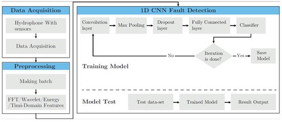
Figure 1.
Flowchart of the proposed methods. 1D-CNN: 1D convolution neural network; FFT: fast Fourier transform.
2.1. Fast Fourier Transform
The Fourier transform was applied to the acoustic signals acquired from hydrophones in healthy and faulty states to obtain the frequency spectrum. The signal’s spectrum is a powerful tool in specifying the tanks’ fault, as it contains all the frequency components. Thus, a burst of bubbles happening randomly could be easily detected and investigated.
Fourier transform is part of the frequency-domain analysis where it decomposes a signal as a function of time into the frequencies that it comprises. Actually, the FFT is called the frequency domain representation of the original signal. The inputs of this transformation are the buckets of data that contain specific numbers of data and are the spatial domain equivalent, while the output is an image in the Fourier or the frequency domain [19]. Having short computational time and capability to extract the most prevalent frequency components of a signal makes this method attractive for most applications. A Fourier transform pair is often written as f(x)↔F(w), or F(f(x)) = F(w), where F is the Fourier transform operator. If f(x) is thought of as a signal (i.e., input data), then it is called F(w) as the signal’s spectrum. The definition of FFT is shown in Equation (1).
A tank in a healthy or a faulty state has different data distributions in the signal’s specification in the fault detection context. The FFTs of healthy and faulty acoustic signals recorded by the hydrophones are depicted in Figure 2. It reveals that, apart from the similarity in major peaks occurring at 200, 400, 600, and 800 Hz for both states, there were minor transient changes visible in the FFT spectrum around 100–150 Hz and 800–900 Hz. In this way, a burst of bubbles, which were happening randomly, could be easily detected and investigated by having access to all the frequency components.
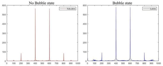
Figure 2.
Comparison of FFT spectrum for healthy and faulty states.
2.2. Wavelet Transform
The wavelet transform (WT) is an efficient time-frequency analysis and a useful tool for signal and image processing applications [20]. The characteristic of the time-frequency analysis technique meets the requirement for analyzing non-stationary signals. The image can be decomposed at different levels of resolution using a wavelet transform. Wavelet decomposition contains different window sizes and can be processed from low resolution to high resolution. In the current study, the wavelet transform was applied to show its efficiency in recognizing leakage in different types of tanks and was compared with other methods. The effects of wavelet with one level of decomposition on the raw input signal in faulty and healthy states are shown in Figure 3 and Figure 4.
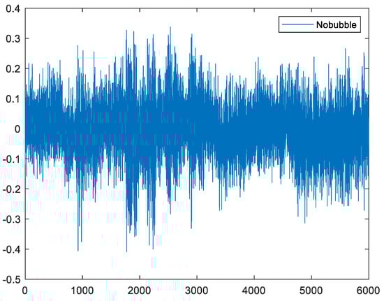
Figure 3.
Wavelet output of a healthy signal.
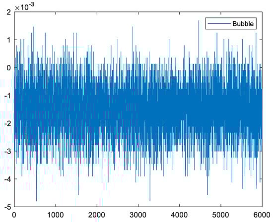
Figure 4.
Wavelet output of a faulty signal.
The wavelet decompositions into approximation and detail coefficients of hydrophone sensor signals in healthy and faulty states are shown in Figure 5. The obtained signals during separate healthy and faulty states of the tank were distinct in wavelet decompositions when they were compared with each other.
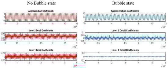
Figure 5.
Comparison of training and test data in terms of accuracy in wavelet_1DCNN.
The above finding reveals that wavelet transforms can also be used as an effective tool for identifying faulty tanks in terms of accuracy, as the experimental results show this method did not provide promising accuracy compared with FFT followed by 1D-CNN. In Table 1, previous research works applying various feature extraction techniques are listed.

Table 1.
Previous research efforts in anomaly detection using three signal-processing techniques.
2.3. Statistical Features
The acoustic emissions obtained from the immersed underwater tank were time-domain measurements of the tank’s activity pressurized at specific time intervals. Analyzing these measurements directly did not yield satisfactory results. Furthermore, the measured signals’ sampling frequency was 100 kHz, and, thus, each sample contained a huge number of data points. Quantification of the acoustic emission (AE) signals’ statistical features was needed to reduce the dimensions of the original data. Using time-domain statistical features greatly reduced computational complexity and discriminated between the signals associated with the feature space’s different structural integrity conditions. All of these benefits were achieved, while FFT followed by 1D-CNN performed better in terms of accuracy. The time-domain statistical features extracted from AE signals in this study consisted of mean value, standard deviation (SD), root mean square (RMS), kurtosis (K), crest factor (C), skewness (S), and peak-to-peak (PPV) values. The mathematical representation of these statistical features is given in Table 2, where xi is the acoustic emission signal.
Table 2.
Statistical time-domain features.
The gained values of statistical features extracted from AE signals are shown in Table 3. These features projected the AE signals into a reduced feature space. Label 1 and label 0 indicate faulty and healthy signals, respectively, where the original matrix was 15,240 × 7.
Table 3.
Statistical features values.
2.4. Convolution Neural Network
In this case study, after feature extraction, it was necessary to utilize a tool that could receive a huge volume of data for processing. Deep-learning technology, particularly the convolutional neural network (CNN), can process the data. CNNs work the same way whether they have one, two, or three dimensions. The difference is the structure of the input data and how the filter moves across the data. In this paper, we proposed applying an accurate fault detection system named 1D-CNN. In 1D-CNN, the kernel moves in one direction, and the input and the output data of that is two-dimensional. It also works well for the analysis of time-series data. Our input data to the 1D-CNN had one channel. The proposed approach could classify the input features samples acquired from the hydrophone sensors and make a prediction model. The 1D-CNN could achieve an elegant classification and fault detection accuracy due to it learning to extract the optimal features and conduct appropriate training. One point to note is that the gained data had a structured type with a leakage failure mode and a crack type of fault. Thus, analysis could be done with a data-driven approach such as 1D-CNN, and there was no need to use a complicated analysis of the tank structure and the physics models.
The convolutional neural network is a multi-stage neural network composed of some filter stages and one classification stage. The filter stage is designed to extract features from the inputs, including the convolution and the pooling layers. The final layer, the classification part, is a multi-layer perceptron composed of several fully connected or dense layers. A dropout layer can also be used between two layers to reduce the model’s complexity and prevent over-fitting. The function of each type of layer [30] has been described as follows.
The convolution layer convolves the input local regions with filter kernels, followed by the activation unit to generate the output features. Each filter uses the same kernel, also known as weight sharing, to extract the local feature of the input local region. One filter corresponds to one frame in the next layer, and the number of frames is called the depth of this layer.
After the convolution operation, activation function can be defined, such as tanh, sigmoid, or relu. Sigmoid layer combines numbers to range of (0 to 1), and it is historically popular in literature. It is common to add a pooling layer after a convolutional layer in the CNN architecture as well. It functions as a down-sampling operation that reduces the spatial size of the features and the network parameters. The most commonly used pooling layer is the max-pooling layer, which performs the local max operation over the input features. It can reduce the parameters and obtain location invariant features at the same time. As mentioned earlier, the dropout layer is added to prevent over-fitting. Over-fitting describes random error or noise instead of the underlying relationship. When a model is excessively complex, such as having too many parameters relative to the number of observations, an over-fitted model has poor predictive performance, as it overreacts to minor fluctuations in the training dataset.
The dense layer is a linear operation in which every input is connected to every output by weight, generally followed by a non-linear activation function such as relu, tanh, or sigmoid. Actually, a dense layer or a fully connected layer classifies the input to the pre-defined labels. In 1D-CNN, kernel slides along one dimension, and data acquired from hydrophones are a type of data that require kernel sliding in only one dimension and that have spatial properties. As one part of deep learning, CNN has a strong mathematical background, which can receive all the signal frequency components and process them. An overview of a sample 1D-CNN includes input signal, convolution layer, max-pooling layer, dropout layer, relu as activation function, fully connected layer, and sigmoid function with binary cross-entropy, which is shown in Figure 6.
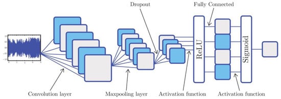
Figure 6.
1D-CNN structure.
3. Experimental Procedure
3.1. Experimental Set-Up
A healthy and a faulty plastic round tank were immersed in a water-filled chamber separately and pressurized with air (0.3 bars) to demonstrate the hydrophone-based detection system, as shown in Figure 7. The selection of hydrophones was critical for detecting bubbles produced by the tanks’ leakage submerged in water. High-quality hydrophones were selected for this task with high sensitivity and wide-band. The shielding against noise was an important aspect of hydrophone selection. The Bruel and Kjaer 8103 hydrophone is suitable for high-frequency laboratory and industrial purposes to collect experimental data.
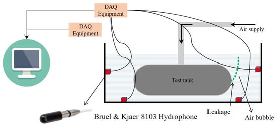
Figure 7.
Schematic illustration of the experimental setup.
Four hydrophones were fused to the Nexus amplifier using BNC (Bayonet Neill–Concelman) connectors. The Nexus amplifier’s output was connected to the national instrument (NI) data acquisition card model 9215, and the sampling rate was configured as 100 K samples. Once the signal was acquired, a digital band-pass filter was applied with cut-off frequencies of 500 Hz to 4 kHz. The hydrophone was situated at a different height from the water’s surface, and data were collected in two different conditions, a healthy state in which we had an intact tank and a faulty state in which we had a crack in the tank. The defected tank had a hole of 70 µm, and the raw signal was collected with a sample rate of 100 kHz. In this experiment, the results from four sensors show us that repeatability was the same for all of them, thus, for data analysis, we applied the output of one of these sensors. One more point to note is that the accuracy of the proposed model does not depend on the sensors’ location. Healthy and faulty signals recorded by these hydrophones are shown in Figure 8 and Figure 9.
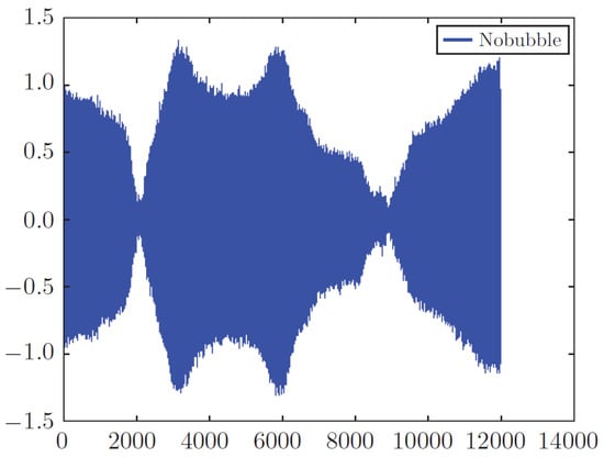
Figure 8.
Raw healthy signal (no bubble).
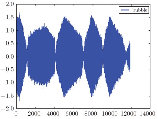
Figure 9.
Raw faulty signal (bubble).
In [31], leakage detection of a spherical water storage tank in a chemical industry using acoustic emissions was investigated. In this paper, four acoustic emission sensors, which are considered expensive sensors in the industry, each with a 1 Mhz sampling rate, were applied. This ensured we created a dataset with high precision in the result, while our analysis was done with the datasets gained from one of these sensors and with the sampling rate of 100 K. Data in our experiment were transmitted to a frequency domain in which failure modes could be identified better and mitigate the dependency of our work on the sensor’s location.
3.2. Dataset and Algorithm
It should be noted that our experiment is considered as a binary classification, and a binary classifier is categorized as an instance of supervised learning. In supervised learning, we have a set of input data and labels, and our task is to map each data point to its specific label. A binary classifier classifies elements into two groups, healthy (no bubble) or faulty (bubble). It is also important to know that the dataset fed into the 1D-CNN model is divided into three groups: training, test, and validation datasets. This classification is that developing a model always involves tuning its configuration, i.e., choosing the number of layers or the size of layers (called the hyper-parameters of the model). The tuning was conducted by using the performance of the model on the validation data. In essence, this tuning is a form of learning—searching for a good configuration in some parameter space.
The training set contained a known output and the model learned on this data to be generalized to other data later on. The validation dataset was used to evaluate our model, and, finally, the test dataset was used to test our model just once. In this paper, as shown in Table 4, we considered 70% of our dataset as training and validation datasets and 30% of the remaining as test datasets.
Table 4.
Statistical time-domain features.
We had 127 samples from two classes. Each sample was a matrix of 1 × 12,000,000 array. The data were organized as each matrix of 1 × 12,000,000 into 120 matrixes of 100,000 arrays (1 × 100,000). We had 15,240 matrixes of 100,000 arrays. This created an excellent dataset for testing our models. We assigned zero to no bubble samples and one to bubble samples. As the number of healthy samples (107 samples) in the sound situation was much higher than the number of faulty ones (20 samples), we equaled the number of healthy and faulty samples to have a fair investigation. In this regard, we used pandas.dataframe.sample to get a random sample of items from an object’s axis with a specific fraction. Here, we used a fraction of 19% on the faulty data. As mentioned earlier, we considered the portion of the training dataset more because we needed to split our training dataset into a training and a validation dataset to tune the hyper-parameters and avoid over-fitting. In this model, we did not need to normalize the datasets, as we had one failure condition, and all the environment parameters were the same for all the methods. We did not have multiple loads to normalize them; we extracted one feature from a fixed condition.
In the following Algorithm 1, the algorithm of FFT-1D-CNN in the form of pseudo-code is given.
| Algorithm 1 Pseudo-code of FFT_1D CNN Algorithm |
| Input: Raw healthy and faulty signals Output: Binary value Step 1: Calling raw input samples (127 samples) one by one, each sample would be as follows: , Where is the vector of 1×12,000,000 over R. Step 2: Extracting the name of each sample Step 3: Assigning 0 and 1 labels to each sample If the filename starts with bubble, then label = 1 else label = 0 Step 4: Splitting each sample into 120 equal size buckets, each bucket would have the following shape: , Where is the vector of 1 × 100,000 over R. Each bucket is obtained during batch processing ((i−1) × Δ + 1) → (I × Δ), where Δ is the sampling rate 100 kHz and i = 1, …, 120, corresponds to the number of batches at time T= 1 sec. Step 5: Calculating FFT of each bucket, the collected FFT values of all buckets (127 × 120) can be arranged in a the matrix as , where is the vector of 15,240 × 1000 over R. Step 6: Making equal the number of healthy and faulty samples so that the FFT matrix size would be 4840 × 1000. Step 7: Specifying training, validation, and test datasets. Each dataset would be as follows: The training dataset is a vector of 2172 × 1000, and the validation dataset would be a vector of 1070 × 1000 Moreover, the test dataset is 1598 × 1000. Step 8: Expanding the shape of training, validation, and test datasets so they would be as follows: The training dataset is a vector of 2172 × 1000 × 1. The validation dataset would be a vector of 1070 × 1000 × 1 Moreover, the test dataset would be 1598 × 1000 × 1. Step 9: Creating a sequential model Step 10: Defining the proper layers
Specifying binary cross-entropy as loss function and Adam as an optimizer, finally calling compile ( ) function on the model Step 12: Fitting the model: A sample of data should be trained by calling the fit ( ) function on the model. Step 13: Making a prediction Generating predictions on new data by calling evaluate ( ) function. The output of this step would be two values, 0 and 1, with their accuracy as follows: If index = 1 then the related value shows the accuracy of fault detection, else it shows healthy accuracy. End |
Two other methods, wavelet and time-domain features followed by 1D-CNN, have the same procedure; only the size of the input matrix for the 1D-CNN model is different because of the impact of the applied method, which creates a different output matrix and needs to act accordingly. The structure of the 1D-CNN and the number of layers is the same in all three signal-processing methods.
Our goal was to achieve a model that generalizes (i.e., performs well on never before seen data), but over-fitting is the central obstacle. What is observed can be controlled; therefore, it is crucial to measure the proposed model’s generalization power. In the following section, over-fitting in our model and the strategy applied to mitigate that and maximize the generalization are shown.
4. Experimental Results and Analysis
A better model on the training data is not necessarily a model that will do better on data it has never seen before. The first plots of validation accuracy and loss showed over-fitting in our model (Figure 10). In precise terms, the following plots were over-fitting in the FFT, followed by the 1D_CNN technique. The training accuracy increased linearly over time until it reached nearly 100%, whereas the validation accuracy stalled at 70–72%. The validation loss reached its minimum after about ten epochs and then started increasing, whereas the training loss kept decreasing linearly until it reached nearly zero. The number of epochs was a hyper-parameter that defined the number of times the learning algorithm worked through the entire training dataset.
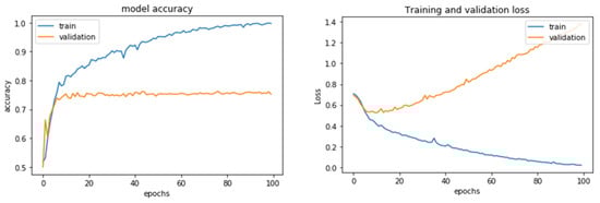
Figure 10.
Accuracy and loss model of FFT_1D-CNN.
Clearly, after the tenth epoch, we had over-optimized the training data and ended learning representations specific to the training data and thus did not generalize to data outside of the training set. In the other two methods, over-fitting before tuning the hyper-parameters was also visible. They are shown in the following plots (Figure 11 and Figure 12).
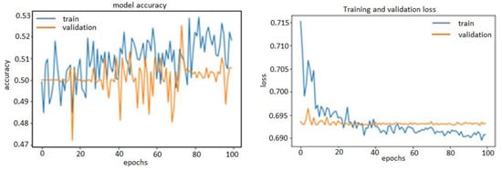
Figure 11.
Accuracy and loss model of time-domain features 1D-CNN.
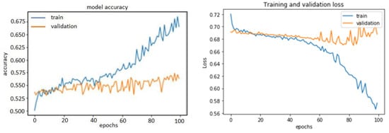
Figure 12.
Accuracy and loss model of wavelet_1D-CNN.
To find the optimal configuration, we needed to regularize the model and tune the hyper-parameters that neither under-fit nor over-fit.
It was required to modify the model, train repeatedly, and evaluate the validation data (not the test data at this point). Several modification items were:
- Adding dropout layers;
- Trying different architectures, e.g., adding or removing layers;
- Adding L1 and/or L2 regularization;
- Trying different hyper-parameters (such as the number of units per layer or the optimizer’s learning rate) to find the optimal configuration;
- Optionally, iterating on feature engineering, e.g., adding new features or removing features that were not informative.
Thanks to L2 regularization and adding dropout layers, our plots were no longer over-fitting; the training curves were closely tracking the validation curves, as is obvious in the figures below from Figure 13, Figure 14 and Figure 15. We obtained an accuracy of about 87% or 88% in the model of FFT_1D-CNN, about 52% in the model of time-domain features_1D-CNN, and, finally, 54% in the model of wavelet_1D-CNN.
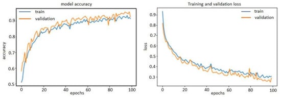
Figure 13.
Accuracy and loss model of FFT_1D-CNN.
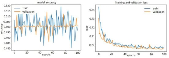
Figure 14.
Accuracy and loss model of time-domain features_1D-CNN.
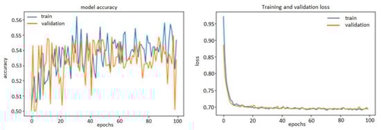
Figure 15.
Accuracy and loss model of Wavelet_1D-CNN.
In this model, we used adaptive moment estimation (Adam) as the main efficient optimization algorithm to update network weights iteratively based on training data. Adam has superiority compared with the other optimizers; it is straightforward to implement, computationally efficient, has few memory requirements, is invariant to diagonal rescale of the gradients, is well suited for problems that are large in terms of data and/or parameters, is appropriate for non-stationary objectives as well as for problems with very noisy/or sparse gradients, and hyper-parameters have intuitive interpretation and typically require little tuning.
We also needed to specify the loss function to evaluate a set of weights. In this case, we used logarithmic loss, which is defined in Keras as binary cross-entropy for a binary classification problem. It is worth mentioning that, in all the mentioned methods, after tuning the hyper-parameters, evaluation was performed by computing the trained model’s accuracy on a held-out validation dataset. Finally, the best hyper-parameter combination in terms of validation accuracy could be tested on a held-out test dataset. A summary of the results regarding changing some hyper-parameters in the 1D-CNN model is mentioned in the Table 5.
Table 5.
Impact of the different parameters and methods on the accuracy of the model.
Stochastic gradient descent (SGD) was not a good optimizer compared with Adam optimizer. In other words, Adam optimizer outperformed every other optimization algorithm. Furthermore, using a smaller dropout value of 20% provided a good starting point. It is worth mentioning that a value of dropout that was too low had minimal effect, and a value too high resulted in under-learning by the network. As specified in Table 6, the total number of layers used in the proposed 1D-CNN architecture was 12.
Table 6.
Structure of the 1D-CNN model.
The summary of the parameters used in the FFT_1D-CNN method is described in Table 7.
Table 7.
Impact of the different parameters on the methods.
“None” in the above table means that it did not have a pre-defined number. For example, it could be the batch size we used during training and made flexible by not assigning any value. Because of this reason, we could change the size of our batch. The model inferred the shape from the context of the layers. The numbers of epochs and batches were also highly dependent on the types and the quantity of input raw data. It means that fewer epochs may lead to the best result for one method, and, for the other, more epochs are required. For the proposed model, various epochs and batches were tested where the epoch’s best number was 100.
In this experiment, the performance of applied methods was analyzed in terms of accuracy. It was observed that 1D-CNN based on FFT had higher prediction accuracy (86.42%) than the other signal processing techniques presented in Table 8. It is interesting to note that, in higher epochs, the accuracy of 1D-CNN based on wavelet overtook the accuracy of 1D-CNN based on time domain features, while FFT-1D-CNN showed its superiority in all different conditions. As mentioned earlier, we did not evaluate our model with the test data for a number of times. We only evaluated once the best model gained from the training and the validation datasets on the test dataset. In the following, the results of evaluation on the test model are mentioned.
Table 8.
The fault detection performance of the proposed methods on the test dataset.
5. Conclusions
This research primarily aimed to detect leakage in fluid tanks after production, virtually using a hydrophone sensor and deep learning algorithm. Acoustic-based leak detection technology is recognized as an effective approach to implementing a true real-time leak monitoring system due to its high leak-detection speed and ease of retrofitting. For improving the prediction model, some other points are worth considering, such as fine-tuning of the hyper-parameters in CNN architecture, which was also done in our work, increasing the sampling rate of sensors, or using expensive sensors which can provide higher precision.
From the engineering perspective, it is acceptable to consider a trade-off between cost and accuracy. The probability of fault with the accuracy of more than 75% is acceptable, while the cost of that experiment is also low.
In this paper, two main phases were done in order to be able to detect the presence of the fault in the plastic tank.
- Three types of feature extraction methods, i.e., FFT transform, wavelet, and time-domain features of the signal, were implemented to differentiate healthy and faulty states.
- 1D-CNN-based architecture was used to determine leakage along with the three different feature extraction methodologies.
Results show that the FFT-based feature extraction technique can effectively detect leakage in plastic and composite tanks. These results were gained by analyzing a dataset from one of these sensors, regardless of its location. Reducing costs and having an acceptable accuracy for detecting leakage can be an achievement in engineering considerations.
Author Contributions
Conceptualization, M.R. and A.A.; methodology, M.R. and A.A.; software, M.R. and A.A.; validation, M.R.; A.A.; M.A. and J.H.; formal analysis, M.R. and A.A.; investigation, M.R.; A.A.; M.A. and J.H.; resources, M.R..; data curation, M.R. and A.A.; writing—original draft preparation, M.R.; writing—review and editing, M.R.; A.A.; M.A. and J.H.; visualization, M.R. and A.A.; supervision, M.R. and A.A.; project administration, A.A.; funding acquisition, M.A. and J.H. All authors have read and agreed to the published version of the manuscript.
Funding
This research received no external funding.
Acknowledgments
The authors would like to thank the team of Smart Infrastructure and Industry Research Group at Manchester Met University for all kinds of support for conducting research and preparing the manuscript.
Conflicts of Interest
The authors declare no conflict of interest.
References
- Giantomassi, A.; Ferracuti, F.; Iarlori, S.; Ippoliti, G.; Longhi, S. Electric motor fault detection and diagnosis by kernel density estimation and kullback–leibler divergence based on stator current measurements. IEEE Trans. Ind. Electron. 2014, 62, 1770–1780. [Google Scholar] [CrossRef]
- Gao, Z.; Cecati, C.; Ding, S.X. A survey of fault diagnosis and fault-tolerant techniques—Part I: Fault diagnosis with model-based and signal-based approaches. IEEE Trans. Ind. Electron. 2015, 62, 3757–3767. [Google Scholar] [CrossRef]
- Dai, X.; Gao, Z. From model, signal to knowledge: A data-driven perspective of fault detection and diagnosis. IEEE Trans. Ind. Inform. 2013, 9, 2226–2238. [Google Scholar] [CrossRef]
- Zhou, W.; Habetler, T.G.; Harley, R.G. Bearing fault detection via stator current noise cancellation and statistical control. IEEE Trans. Ind. Electron. 2008, 55, 4260–4269. [Google Scholar] [CrossRef]
- Schoen, R.; Habetler, T.; Kamran, F.; Bartfield, R. Motor bearing damage detection using stator current monitoring. IEEE Trans. Ind. Appl. 1995, 31, 1274–1279. [Google Scholar] [CrossRef]
- Kliman, G.B.; Premerlani, W.J.; Yazici, B.; Koegl, R.A.; Mazereeuw, J. Sensor-less, online motor diagnostics. IEEE Comput. Appl. Power 1997, 10, 39–43. [Google Scholar] [CrossRef]
- Pons-Llinares, J.; Antonino-Daviu, J.A.; Riera-Guasp, M.; Bin Lee, S.; Kang, T.-J.; Yang, C. Advanced induction motor rotor fault diagnosis via continuous and discrete time–frequency tools. IEEE Trans. Ind. Electron. 2014, 62, 1791–1802. [Google Scholar] [CrossRef]
- Arthur, N.; Penman, J. Induction machine condition monitoring with higher order spectra. IEEE Trans. Ind. Electron. 2000, 47, 1031–1041. [Google Scholar] [CrossRef]
- Benbouzid, M.; Vieira, M.; Theys, C. Induction motors’ faults detection and localization using stator current advanced signal processing techniques. IEEE Trans. Power Electron. 1999, 14, 14–22. [Google Scholar] [CrossRef]
- Li, D.Z.; Wang, W.; Ismail, F. An enhanced bi-spectrum technique with auxiliary frequency injection for induction motor health condition monitoring. IEEE Trans. Instrum. Meas. 2015, 64, 2679–2687. [Google Scholar] [CrossRef]
- Eren, L.; Devaney, M.J. Bearing damage detection via wavelet packet decomposition of the stator current. IEEE Trans. Instrum. Meas. 2004, 53, 431–436. [Google Scholar] [CrossRef]
- Ye, Z.; Wu, B.; Sadeghian, A. Current signature analysis of induction motor mechanical faults by wavelet packet decomposition. IEEE Trans. Ind. Electron. 2003, 50, 1217–1228. [Google Scholar] [CrossRef]
- Kiranyaz, S.; Ince, T.; Gabbouj, M. Real-Time patient-specific ECG classification by 1-D convolutional neural networks. IEEE Trans. Biomed. Eng. 2015, 63, 664–675. [Google Scholar] [CrossRef]
- Ince, T.; Kiranyaz, S.; Eren, L.; Askar, M.; Gabbouj, M. Real-Time motor fault detection by 1-D convolutional neural networks. IEEE Trans. Ind. Electron. 2016, 63, 7067–7075. [Google Scholar] [CrossRef]
- Cataldo, A.; Cannazza, G.; De Benedetto, E.; Giaquinto, N. A new method for detecting leaks in underground water pipelines. IEEE Sens. J. 2011, 12, 1660–1667. [Google Scholar] [CrossRef]
- Giaquinto, N.; D’Aucelli, G.M.; De Benedetto, E.; Cannazza, G.; Cataldo, A.; Piuzzi, E.; Masciullo, A. Criteria for automated estimation of time of fight in tdr analysis. IEEE Trans. Instrum. Meas. 2016, 65, 1215–1224. [Google Scholar] [CrossRef]
- Knapp, C.; Carter, G. The generalized correlation method for estimation of time delay. IEEE Trans. Acoust. Speech Signal Process. 1976, 24, 320–327. [Google Scholar] [CrossRef]
- Hero, A.; Schwartz, S. A new generalized cross correlator. IEEE Trans. Acoust. Speech Signal Process. 1985, 33, 38–45. [Google Scholar] [CrossRef]
- Li, B.; Chow, M.-Y.; Tipsuwan, Y.; Hung, J. Neural-network-based motor rolling bearing fault diagnosis. IEEE Trans. Ind. Electron. 2000, 47, 1060–1069. [Google Scholar] [CrossRef]
- Pandiyan, V.; Tjahjowidodo, T. In-process endpoint detection of weld seam removal in robotic abrasive belt grinding process. Int. J. Adv. Manuf. Technol. 2017, 93, 1699–1714. [Google Scholar] [CrossRef]
- Kwak, J.-S.; Ha, M.-K. Neural network approach for diagnosis of grinding operation by acoustic emission and power signals. J. Mater. Process. Technol. 2004, 147, 65–71. [Google Scholar] [CrossRef]
- Al-Habaibeh, A.; Gindy, N. A new approach for systematic design of condition monitoring systems for milling processes. J. Mater. Process. Technol. 2000, 107, 243–251. [Google Scholar] [CrossRef]
- Niu, Y.M.; Wong, Y.S.; Hong, G.S. An intelligent sensor system approach for reliable tool flank wear recognition. Int. J. Adv. Manuf. Technol. 1998, 14, 77–84. [Google Scholar] [CrossRef]
- Betta, G.; Liguori, C.; Paolillo, A.; Pietrosanto, A. A DSP-based FFT-analyzer for the fault diagnosis of rotating machine based on vibration analysis. IEEE Trans. Instrum. Meas. 2002, 51, 1316–1322. [Google Scholar] [CrossRef]
- Rai, V.; Mohanty, A. Bearing fault diagnosis using _t of intrinsic mode functions in Hilbert-huang transform. Mech. Syst. Signal Process. 2007, 21, 2607–2615. [Google Scholar] [CrossRef]
- Pandiyan, V.; Caesarendra, W.; Tjahjowidodo, T.; Tan, H.H. In-process tool condition monitoring in compliant abrasive belt grinding process using support vector machine and genetic algorithm. J. Manuf. Process. 2018, 31, 199–213. [Google Scholar] [CrossRef]
- Sohn, H.; Park, G.; Wait, J.R.; Limback, N.P.; Farrar, C.R. Wavelet-based active sensing for delamination detection in composite structures. Smart Mater. Struct. 2003, 13, 153–160. [Google Scholar] [CrossRef]
- Hou, Z.; Noori, M.; Amand, R.S. Wavelet-Based approach for structural damage detection. J. Eng. Mech. 2000, 126, 677–683. [Google Scholar] [CrossRef]
- Yang, H.-T.; Liao, C.-C. A de-noising scheme for enhancing wavelet-based power quality monitoring system. IEEE Trans. Power Deliv. 2001, 16, 353–360. [Google Scholar] [CrossRef]
- LeCun, Y. Deep learning and convolutional networks. In Hot Chips 27 Symposium (HCS); IEEE: New York, NJ, USA, 2015; pp. 1–95. [Google Scholar]
- Sohaib, M.; Islam, M.; Kim, J.; Jeon, D. Leakage Detection of a Spherical Water Storage Tank in a Chemical Industry Using Acoustic Emissions. Appl. Sci. 2019, 9, 196. [Google Scholar] [CrossRef]


Publisher’s Note: MDPI stays neutral with regard to jurisdictional claims in published maps and institutional affiliations. |
© 2020 by the authors. Licensee MDPI, Basel, Switzerland. This article is an open access article distributed under the terms and conditions of the Creative Commons Attribution (CC BY) license (http://creativecommons.org/licenses/by/4.0/).