Article

Finding Good Attribute Subsets for Improved Decision Trees Using a Genetic Algorithm Wrapper; a Supervised Learning Application in the Food Business Sector for Wine Type Classification

by
Dimitris C. Gkikas
1,*,
Prokopis K. Theodoridis
2,
Theodoros Theodoridis
3 and
Marios C. Gkikas
4
1
Department of International & European Economic Studies, School of Economic Sciences, Athens University of Economics and Business, 76 Patision Str., 10434 Athens, Greece
2
School of Social Sciences, Hellenic Open University, Patras Campus, 18 Aristotelous Str., 26335 Patras, Greece
3
School of Science Engineering and Environment, University of Salford, The Crescent, Salford M5 4WT, UK
4
Department of Management Science and Technology, School of Economics and Business, University of Patras, 1 M. Alexandrou Str., Koukouli, 26334 Patras, Greece
*
Author to whom correspondence should be addressed.
Informatics 2023, 10(3), 63; https://doi.org/10.3390/informatics10030063
Submission received: 13 April 2023 / Revised: 24 June 2023 / Accepted: 3 July 2023 / Published: 21 July 2023
(This article belongs to the Special Issue Applications of Machine Learning and Deep Learning in Agriculture)

Abstract

:
This study aims to provide a method that will assist decision makers in managing large datasets, eliminating the decision risk and highlighting significant subsets of data with certain weight. Thus, binary decision tree (BDT) and genetic algorithm (GA) methods are combined using a wrapping technique. The BDT algorithm is used to classify data in a tree structure, while the GA is used to identify the best attribute combinations from a set of possible combinations, referred to as generations. The study seeks to address the problem of overfitting that may occur when classifying large datasets by reducing the number of attributes used in classification. Using the GA, the number of selected attributes is minimized, reducing the risk of overfitting. The algorithm produces many attribute sets that are classified using the BDT algorithm and are assigned a fitness number based on their accuracy. The fittest set of attributes, or chromosomes, as well as the BDTs, are then selected for further analysis. The training process uses the data of a chemical analysis of wines grown in the same region but derived from three different cultivars. The results demonstrate the effectiveness of this innovative approach in defining certain ingredients and weights of wine’s origin.

1. Introduction

As an essential preprocessing stage for machine learning, feature selection endeavors to identify significant predictors from a feature-rich dataset with high dimensionality. The primary objective is to enhance prediction accuracy by selecting the most representative features. This study presents an innovative strategy that integrates binary decision trees and genetic algorithms to effectively handle extensive datasets and support informed decision making. The purpose of this algorithm is to use a GA as classifier system to find an optimized tree structure along with an optimal terminal set of a BDT, and to promote and select the elitist as a solution, which will enable the classification of datasets by undergoing a training, validation, and testing phase, along with an ensemble method that combines multiple BDT structures to improve classification performance.
This approach utilizes binary decision trees (BDTs) for classification purposes and genetic algorithms (GAs) for selecting the most optimal attributes, thus minimizing the likelihood of overfitting. The experimental application of this methodology to wine chemical analysis yields promising outcomes. The combination of binary decision trees and genetic algorithms offers a novel solution for managing significant subsets of wine data with assigned weights using a machine learning model through a multi-disciplinary approach, testing it on real-world chemical substance data, and refining it. It also offers valuable insights for future work with a human-centric perspective. To achieve this, machine learning classification utilizing an optimization method is employed to gather valid information from this specific field of interest. The identification of wine types necessitates an understanding of how respondents’ answers correspond to three distinct classes: 1, 2, and 3. The outcomes reveal subsets of attributes that effectively replace the initial attribute set, achieving high accuracy/fitness levels (above 80%) with varying numbers of attributes based on the class. It is important to clarify that this study encompasses two distinct decision-making processes. The first relates to the chemical substances which identify the wine’s origin, while the second pertains to the core analysis conducted using machine learning to generate results minimizing the risk of decision.
AI-supervised learning is employed to analyze wine data and predict the factors influencing a wine’s type. The data is extracted from the Institute of Pharmaceutical and Food Analysis and Technologies in Italy. The primary objective of this study is to examine, process, classify, and evaluate datasets to generate reliable insights regarding the chemical substances which are responsible for determining a wine’s origin. Thirteen continuous variables—Alcohol, Malic Acid, Ash, Alkalinity of Ash, Magnesium, Total Phenols, Flavonoids, Nonflavonoid Phenols, Proanthocyanins, Color Intensity, Hue, OD280/OD315 of Diluted Wines, and Proline—refer to the chemical substances that classify a wine’s type [1].
This study addresses the challenge of hybrid data classification by introducing an optimization population-based metaheuristic method that combines two distinct methods and a programming technique into a unified entity. The BDT algorithm is used for data classification, while the GA algorithm is used for optimization, and the wrapping technique facilitates communication and data exchange between the two methods. This model uses BDTs to efficiently handle, categorize, and extract insights from raw data, resulting in precise subsets of data instead of using the entire set of features. It is tested in different conditions, including various numbers and types of features, record numbers, and industry contexts. The goal is to generate optimal feature subsets that reduce processing time and improve prediction accuracy. The algorithm’s logic is explained, and the best attribute subsets are presented using graphs and histograms.
While the proposed machine learning model integrating a GA wrapper with BDTs demonstrates promising results in classifying the wine substances that affect the wine’s origin, it is important to acknowledge certain limitations and consider further avenues for exploration. The current study focused on a specific dataset from the wine industry, limiting the generalizability of the findings to other domains. Future research could expand the scope by incorporating diverse datasets from various industries to assess the model’s applicability and performance in different contexts. Following, the wine industry is known for its dynamic nature, characterized by evolving production techniques and regional variations. To enhance the practicality and relevance of the model, it would be valuable to explore its adaptability to these dynamic factors. Investigating how the model can effectively capture and adapt to changes in winemaking practices, as well as variations in regional characteristics, could provide deeper insights into its robustness and generalizability. In addition to improving the model’s practical application, the study could further investigate the interpretability and explainability of the model’s decision-making process. While the accuracy and performance of the model are crucial, understanding the underlying factors and features that contribute to its predictions is equally important. By incorporating interpretability techniques, researchers and domain experts can gain insights into which wine substances play a dominant role in determining the wine’s origin, facilitating the validation and acceptance of the model in real-world scenarios.

2. Related Work

The current research attempt discusses the use of hybrid machine learning in wine data. Thus, the field of study combines the machine learning model implementation stages and its contribution to the wine industry. The literature review part refers to both machine learning and wine decision making.
Referring to the cases where machine learning was introduced in a wine field of study, there are a series of publications that verify its use. To begin with, research was conducted aiming to use a large generic wine dataset to classify and highlight the differences in wines around the world. A world wine dataset, the X-Wines dataset, was created, including data from user reviews and ratings for recommendation systems, machine learning and data mining, and general purposes, opening the way to researchers and students to use it freely. Using evaluation metrics, this project involved data collection, dataset description, training, verification, and validation, and results measurement [2].
Another significant approach [3] referred to a machine learning application in wine quality prediction. The excellence of New Zealand Pinot noir wine led a team of researchers to use machine learning algorithms to predict wine quality by using synthetic and available experimental data collected from different regions of New Zealand. An Adaptive Boosting (AdaBoost) classifier showed 100% accuracy when trained and evaluated without feature selection, with feature selection (XGB), and with essential variables (features found important in at least three feature selection methods) [3].
Another study [4] examined the performance of different machine learning models, namely Ridge Regression (RR), Support Vector Machine (SVM), Gradient Boosting Regressor (GBR), and multi-layer Artificial Neural Network (ANN), was compared for the prediction of wine quality. An analysis of multiple parameters that determine wine quality was conducted. It was observed that the performance of GBR surpassed that of all other models, with mean squared error (MSE), correlation coefficient (R), and mean absolute percentage error (MAPE) values of 0.3741, 0.6057, and 0.0873, respectively. This work demonstrates how statistical analysis can be utilized to identify the key components that primarily influence wine quality prior to production. This information can be valuable for wine manufacturers in controlling quality before the wine production process [4].
Regarding the application of machine learning methods to the wine industry, there is a series of significant research attempts which verifies that the proper use of advanced statistics can mitigate the decision error and provide valid information on wine products. Previous research [5,6] has shown that GAs and BDTs have been utilized together in various optimization and classification tasks in recent decades, as evidenced by the existing literature. The GA wrapper, also used for user authentication through keystroke dynamics, involves analyzing a person’s typing pattern to determine whether to grant or deny access. This was achieved by creating a timing vector that consists of keystroke duration and interval times. However, deciding which features to use in a classifier was a common feature selection issue. One potential solution was a genetic-algorithm-based wrapper approach, which not only resolves the problem but also generates a pool of effective classifiers that can be used as an ensemble. The preliminary experiments demonstrate that this approach outperforms both the two-phase ensemble selection approach and the prediction-based diversity term approach [5,6] (pp. 654–660).
Another study [7] focused on the development of an automated algorithm for feature subset selection in unlabeled data, where two key issues were identified: the identification of the appropriate number of clusters in conjunction with feature selection, and the normalization of feature selection criteria bias with respect to dimensionality. Thus, the Feature Subset Selection using Expectation-Maximization (EM) clustering (FSSEM) approach and the evaluation of candidate feature subsets using scatter separability and maximum likelihood criteria were developed. Proofs were provided on the biases of these feature criteria concerning dimensionality, and a cross-projection normalization scheme to mitigate these biases was proposed. The results show the necessity of feature selection and the importance of addressing these issues, as well as the efficacy of this proposed solution [7].
Another study [8] introduced a novel wrapper feature selection algorithm, referred to as the hybrid genetic algorithm (GA) and extreme learning machine (ELM)-based feature selection algorithm (HGEFS) for classification problems. This approach employed GA to wrap ELM and search for optimal subsets in the extensive feature space. The selected subsets were then utilized for ensemble construction to enhance the final prediction accuracy. To prevent GA from being stuck in local optima, an efficient and innovative mechanism was proposed specifically designed for feature selection issues to maintain the GA’s diversity. To evaluate the quality of each subset fairly and efficiently, a modified ELM known as the error-minimized extreme learning machine (EM-ELM) was adopted, which automatically determines the appropriate network architecture for each feature subset. Moreover, EM-ELM exhibits excellent generalization capability and extreme learning speed, enabling the execution of wrapper feature selection procedures affordably. In other words, the feature subset and classifier parameters were optimized simultaneously. After concluding the GA’s search process, a subset of EM-ELMs from the obtained population based on a specific ranking and selection strategy was selected to improve the prediction accuracy and achieve a stable outcome. To evaluate HGEFS’s performance, empirical comparisons were carried out on various feature selection methods and HGEFS using benchmark data sets. The outcomes demonstrate that HGEFS was a valuable approach for feature selection problems and consistently outperformed other algorithms in comparison [8].
The approach of using multiple classifiers to solve a problem, known as an ensemble, has been found to be highly effective for classification tasks. One of the fundamental requirements for creating an effective ensemble was to ensure both diversity and accuracy. In this study, a new ensemble creation technique that utilized GA wrapper feature selection was introduced. These experimental results on real-world datasets demonstrated that the proposed method was promising when the training data size was restricted [9] (pp. 111–116).
A different study [9] employed a GA hybrid to pinpoint a subset of attributes that were most relevant to the classification task. The optimization process was composed of two stages. During the outer optimization stage, a wrapper method was employed to conduct a global search for the most optimal subset of features. In this stage, the GA employs the mutual information between the predictive labels of a trained classifier and the true classes as the fitness function. The inner optimization stage involves a filter approach to perform local search. In this stage, an enhanced estimation of the conditional mutual information was utilized as an independent measure for feature ranking, taking into account not only the relevance of the candidate features to the output classes but also their redundancy with the already-selected features. The inner and outer optimization stages work together to achieve high global predictive accuracy as well as high local search efficiency. The experimental results demonstrate that the method achieves parsimonious feature selection and excellent classification accuracy across various benchmark data sets [10] (pp. 1825–1844).
The concept of feature set partitioning expands on the task of feature selection by breaking down the feature set into groups of features that were collectively valuable, rather than pinpointing one individual set of features that was valuable. One research paper introduced a fresh approach to feature set partitioning that relied on a GA. Additionally, a new encoding schema was suggested, and its characteristics were explored. The study investigated the effectiveness of utilizing a Vapnik-Chervonenkis dimension bound to assess the fitness function of multiple tree classifiers that were oblivious. To evaluate the new algorithm, it was applied to various datasets, and the outcomes indicate that the proposed algorithm outperforms other methods [11] (pp. 1676–1700).
“Comparison of Naive Bayes and Decision Tree on Feature Selection Using Genetic Algorithm for Classification Problem” stands out as the most significant work in demonstrating the effectiveness of combining DTs and GAs. That study specifically addressed the challenge of identifying optimal attribute classifications through the utilization of a GA and wrapping technique. The focus was on handling large datasets and determining the attributes that have an impact on result quality by considering factors such as irrelevance, correlation, and overlap. The study employed a combination of a DT and Naïve Bayes theorem as the most suitable models for the task. Initially, the DT was integrated with the GA wrapper, resulting in the GADT, which provided classification results. Subsequently, the Naïve Bayes model was also combined with the GA wrapper, leading to GANB for classification optimization. The research team thoroughly discussed how both NB and DT models address the classification problem by leveraging the GA’s ability to identify the best attribute subsets. The performance of each model was comparable, although the comparative analysis revealed that GADT slightly outperformed GANB in terms of accuracy [12].
During the financial crisis of 2007, an alternative method for selecting features was employed in credit scoring modeling. Credit scoring modeling aims to accurately assess the credit risk of applicants using customer data from banks. This particular method was utilized to identify credit risks within the banking sector, eliminating irrelevant credit risk features and enhancing the accuracy of the classifier. The approach involved a two-stage process, combining a hybrid feature selection filter approach with multiple population genetic algorithms (MPGA). In the first stage, three filter wrapper approaches were employed to gather information for the MPGA. The second stage utilized the characteristics of MPGA to identify the optimal subset of features. A comparison was conducted among the hybrid approach based on the filter approach and MPGA (referred to as HMPGA), MPGA alone, and standard GA. The results demonstrated that HMPGA, MPGA, and GA outperformed the three filter approaches. Furthermore, it was established that HMPGA yielded superior results compared to both MPGA and GA [13].
In various industries, including medicine and healthcare, two predominant machine learning approaches have emerged: supervised learning and transfer learning. These methodologies heavily rely on vast manually labeled datasets to train increasingly sophisticated models. However, this reliance on labeled data leads to an abundance of un-labeled data that remains untapped in both public and private data repositories. Addressing this issue, self-supervised learning (SSL) emerged as a promising field within machine learning, capable of harnessing the potential of unlabeled data. Unlike other machine learning paradigms, SSL algorithms generate artificial supervisory signals from unlabeled data and employ these signals for pretraining algorithms. One study dealt with two primary objectives. Firstly, it aimed to provide a comprehensive definition of SSL, categorizing SSL algorithms into four distinct subsets and conducting an in-depth analysis of the latest advancements published within each subset from 2014 to 2020. Secondly, the review focused on surveying recent SSL algorithms specifically in the healthcare domain. This endeavor aimed to equip medical professionals with a clearer understanding of how SSL could be integrated into their research efforts, with the ultimate goal of leveraging the untapped potential of unlabeled data [14].
This article [15] presents a multicriteria programming model aimed at optimizing the completion time of homework assignments by school students in both in-class and online teaching modes. The study defined twelve criteria that influence the effectiveness of school exercises, five of which pertain to the exercises themselves and the remaining seven to the conditions under which the exercises are completed. The proposed solution involves designing a neural network that outputs influence on the target function and employs three optimization techniques—backtracking search optimization algorithm (BSA), particle swarm optimization algorithm (PSO), and genetic algorithm (GA)—to search for optimal values. The article suggests representing the optimal completion time of homework as a Pareto set [15].
The problem of feature subset selection involves selecting a relevant subset of features for a learning algorithm to focus on, while disregarding the others. To achieve the best performance possible with a specific learning algorithm on a given training set, it is important for a feature subset selection method to consider how the algorithm and training set interact. Another study examined the relationship between optimal feature subset selection and relevance. The proposed wrapper method searched for an optimal feature subset tailored to a specific algorithm and domain. The strengths and weaknesses of the wrapper approach were analyzed, and several improved designs were presented. The wrapper approach was compared to induction without feature subset selection and to Relief, which is a filter-based approach to feature subset selection [16].
In many real-world applications of classification learning, irrelevant features are often present, posing a challenge for machine learning algorithms. Nearest-neighbor classification algorithms have shown high predictive accuracy in many cases but are not immune to the negative effects of irrelevant features. A new classification algorithm, called VFI5, has been proposed to address this issue. In this study, the authors compared the performance of the nearest-neighbor classifier and the VFI5 algorithm in the presence of irrelevant features. The comparison was conducted on both artificially generated and real-world data sets obtained from the UCI repository. The results show that the VFI5 algorithm achieves comparable accuracy to the nearest-neighbor classifier while being more robust to irrelevant features [17].

2.1. Research Objectives

The current study was developed to generate more accurate predictions using a GA wrapper for optimal feature selection in decision trees. This model utilizes two distinct methods and a programming technique to create precise subgroups of data, rather than relying on the complete set of features. It combines BDT data classification and GA optimization algorithms to select optimal data features and communicate through wrapping.
The application is capable of analyzing, handling, categorizing, optimizing, and extracting new knowledge from raw data. The application was tested under different feature types and numbers, record numbers, industry contexts, and fields. The objective was to generate an optimal subset of features that reduce processing time while increasing prediction accuracy. The algorithm’s rationale is elaborated, and the best attribute subsets are displayed in performance charts, histograms, and tree graphs. This study is pioneering in its combination of GA with classification algorithms, as such collaborations are rare. In order to ascertain whether the new model can surpass GAs and BDTs, it is necessary to undertake multiple stages, such as presenting, explaining, training, validating, testing, and evaluating the model. The empirical investigation comprises three phases, with the first focusing on the design and analysis of the GA wrapper. The second phase refers to the GA wrapper development and its advantages, while the third phase examines the its performance using multiple datasets for training, validation, testing, and visualization, and generation of average fitness, best fitness, best chromosome gene sequence, and optimal and dominant BDTs. The AI-supervised learning was applied on wine data to predict the factors which affect wine’s different cultivars. The generated results indicate subsets of attributes which replace the initial entire set of attributes, achieving high accuracy/fitness, which consist of different numbers of attributes per class. The study has three main research objectives, each consisting of multiple stages to examine the GA wrapper model design, implementation, and performance (Table 1).
RO1 focuses on the GA wrapper model design and consists of two stages: RO1.1 defines the GA wrapper analysis, while RO1.2 defines the GA wrapper design. RO2 examines the GA wrapper model implementation and consists of five stages: GA wrapper development (RO2.1), GA wrapper training (RO2.2), GA wrapper validation (RO2.3), GA wrapper testing (RO2.4), and GA wrapper representation (RO2.5). RO3 focuses on examining the GA wrapper model’s performance on various datasets and generating a set of decision-making rules. This objective consists of ten stages: GA wrapper to new data (RO3.1), calculating class errors (RO3.2), calculating generation fitness (RO3.3), calculating best fitness (RO3.4), calculating optimal BDTs (RO3.5), visualizing dominant BDTs (RO3.6), calculating the best chromosome’s gene sequence (RO3.7), graphically representing the generations’ fitness (RO3.8), calculating and representing the average chromosome’s gene frequencies (RO3.9), and generating rules for wine origin (RO3.10) (Table 1).

3. Research Methodology

3.1. Research Scope

A GA wrapper is a metaheuristic optimization algorithm that is used to optimize the hyperparameters of a machine learning model. It works by using the principles of natural selection and genetics to iteratively search for the optimal set of hyperparameters. The GA wrapper starts by randomly generating a set of initial hyperparameters for the machine learning model. These hyperparameters are then evaluated based on a fitness function that measures how well the model performs on a validation set. Then, the GA wrapper uses the principles of natural selection to select the best-performing hyperparameters for reproduction. These hyperparameters are then used to generate a new set of hyperparameters through the application of genetic operators, such as crossover and mutation. The process of selection, reproduction, and mutation is repeated for multiple generations, with each generation producing a new set of hyperparameters that are evaluated using the fitness function. Over time, the GA wrapper converges on a set of hyperparameters that optimize the performance of the machine learning model on the validation set. In summary, a GA wrapper is a powerful optimization technique that can be used to efficiently search for the optimal set of hyperparameters for a machine learning model.

3.2. Method Overview

The study initially started with the goal of extracting wine type predictions to provide fast and accurate suggestions. The significance of this application lies in the fact that although DTs are commonly employed for classification tasks, they encounter difficulties in representing data [18,19,20]. To address this issue, the proposed method employs a GA wrapper to identify the attributes that play a significant role in the classification process. This method involves the use of two interconnected algorithms: the GA, which is an optimization algorithm, and the BDT, which is a non-pruned classification algorithm. These algorithms work together in a parallel data processing framework. The GA selects the best attributes from a dataset for the BDT algorithm, presented in a tree structure, achieving comparable accuracy to fully developed BDTs [16,21]. The GA finds and selects the best combinations of attributes to be classified by the BDT. For each combination of attributes, the BDT classifies it and returns a fitness number to the genetic algorithm, which defines the quality of that combination. This process is repeated several times, and the GA returns to the BDT algorithm a combination of attributes that is represented in a tree structure. The wrapping method handles the communication between the BDT and GA and makes it seem like they are executing simultaneously. The utilization of parallel processing on data guarantees the prevention of overfitting, showcasing the optimal set of attributes or genes through tree form representation that depicts the classification accuracy for training, validation, and testing data [22,23].

3.3. Information Gain

The Shannon function is an essential component of the decision tree algorithm, as it helps to determine the usefulness of each attribute in terms of the amount of information it can provide in bits. This function is analogous to the fitness function used in genetic algorithms, which evaluates the overall health of a chromosome. The Shannon function takes into account the existing knowledge about the attribute and evaluates its consistency with that knowledge. When an attribute provides a large amount of information, the value returned by the Shannon function will be lower. This function calculates the amount of information gained from splitting a dataset based on a particular attribute [24].
The amount of information gained is measured in bits, and the mathematical formula used to calculate the Shannon function is as follows:
I ( P ( u 1 ) , ,   P ( u n ) ) = i = 1 n P ( u i )   l o g 2 P ( u i )
where  I ( P ( u 1 ) , ,   P ( u n ) )  represents the amount of information gained by splitting the dataset based on attributes,  P ( u 1 ) , ,   P ( u n ) , and  P ( u )  represents the proportion of the dataset belonging to each class after the split, and P( u i )    is the probability of the possible answer ( u i ) .
R e m a i n d e r   ( A ) = i = 1 u p i + n i p + n   I (   p i p i + n i ,   n i p i + n i )
G a i n   ( A ) = I ( p i p i + n i ,   n i p i + n i ) R e m a i n d e r   ( A )
In addition to the Shannon function, other measures such as the Gini index and the Chi-squared test can also be used to evaluate the information gain of attributes. These measures take into account different aspects of the data, and the selection of the most appropriate measure largely depends on the specific problem at hand. Overall, the selection of an appropriate measure for evaluating information gain is crucial for building accurate decision trees that can effectively classify and predict outcomes (Table 2) [24].

3.4. GA Wrapper Fitness Model

The evaluation of chromosome fitness and its mechanical implementation is a crucial aspect of this study. In essence, the fitness number and accuracy are interchangeable terms used to describe the same numerical value. The chromosome undergoes a classification process via a decision tree, with the accuracy of each chromosome being determined and subsequently returned to the genetic algorithm. At the conclusion of each generation, the overall fitness number is determined.
Each chromosome is composed of 14 genes, and an additional 2 genes are allocated for classification purposes, given the potential for instances to be classified into multiple classes. The number of genes may vary due to the nature of the experimental datasets. The accuracy calculation process is carried out for each instance of the dataset, with the binary decision trees (BDTs) being responsible for settling on the terminals of each calculation [20,24].
The BDTs are made up of predicates and arithmetic symbols that perform the necessary calculations to determine the index of the cell of each instance. The index value serves as an indication of how close the classification made is to the actual class.
Occasionally, an instance may be assigned to multiple classes. Additional votes are given to the BDTs that accurately classify instances, and those with the highest vote count are considered to have played a more significant role in the classification process. The accuracy of the classification process is determined by dividing the number of correctly classified examples by the total number of classified examples. This value serves as the fitness function of the chromosome, which is stored in an array until all instances are classified. The training, validation, and testing data all undergo the same classification procedure, with the maximum and average fitness of the chromosomes being calculated for the population of the last generation only. The validation and testing data have almost the same classification accuracy/fitness (Figure 1) [24,25].

3.5. GA Wrapper Model Design

To define the role and design of the first level of this application, information system diagrams are utilized. These diagrams explain how information flows between functions and depict the procedures that contribute to the application’s development. In this work, flowcharts and sequence diagrams are deemed crucial to acquaint the reader with the model. The flowchart, abstract dataflow diagram, and sequence diagram illustrate the background processes. The flowchart displays the fundamental functions of the study, including processes, functions, and messages exchanged among different parts. The article explains the functioning of the genetic algorithm and its connection to binary decision trees. The wrapping method, which is an integral component of the implementation, cannot be demonstrated independently of the complete application (Figure 2) [26,27].

3.6. GA Wrapper Analysis

To define the role and design of the first level of the application, information system diagrams are utilized. These diagrams illustrate how information flows across functions and indicate the procedures that contribute to the development. Specifically, in this work, flowcharts and sequence diagrams are deemed essential for introducing the model to readers. The flowchart, abstract dataflow diagram, and sequence diagram describe the backstage processes, showing the basic functions, processes, functions, and messages that are sent among different parts of the study. They explain how the genetic algorithm (GA) works and how BDTs are associated with it. The wrapping method is part of the implementation and cannot be demonstrated separately from the entire application (Figure 2 and Figure 3) [26,27].
To create the population of chromosomes for the first generation, the GA reads the dataset attributes and randomly generates chromosomes. Some chromosomes may contain duplicate attributes. The production of subsequent generations involves the implementation of the tournament selection method, mutation, crossover, and selection of the fittest method (Figure 4) [26,27].
The tournament variable is related to the tournament selection process that was described earlier. When utilizing the tournament selection approach, the algorithm randomly picks a certain number of chromosomes from the entire population during the initial phase. The number of chromosomes is determined by the user assigning a number to the tournament variable (e.g., tournament = 4). From this set of chromosomes, the GA chooses the one with the highest fitness score, which remains in the first generation, and the tournament is run again until a set of 100 chromosomes is complete for the 1st generation. In this work, tournament selection is used instead of roulette selection. Once two chromosomes or genes are selected from the first two runs, the mutation or crossover processes may occur to generate two new chromosomes (Figure 4) [26,27].
The likelihood of a gene being modified during the genetic algorithm’s operation is determined by the gene_prob variable, which is fixed at 0.3. If the random number generated by the algorithm is lower than the gene_prob value, the gene will be subject to evolution. The operator_prob variable is responsible for generating random numbers to determine whether the genes of the first two selected chromosomes will undergo mutation or crossover. If the randomly generated number is less than 0.4, either mutation or crossover will occur. There is a 40% chance of crossover happening and a 60% chance of mutation taking place.
The best chromosome resulting from these procedures is stored in an array. Once the array is filled with 100 evolved or unevolved chromosomes, the second generation is created. Subsequent generations are created in the same way as the second. The user can change the operator_prob and gene_prob variables, as well as the population and generation variables, which respectively determine the size of the chromosome population for each generation and the number of generations. Initially, the plan for the BDT algorithm was to develop the application based on the original DT theory that uses mathematical formulas such as the Shannon function.
However, an alternative approach was taken instead of the standard DT algorithm, using a type of DTs known as binary DTs. These DTs are also referred to as ensemble full BDTs, and they are completely symmetrical trees with all their nodes reaching the terminals. The depth of the tree is set to 4 and there is a variable named max_dt in the code, which determines the number of DTs created and involved in the classification process. Although the sizes of the trees are fixed, the user has the ability to adjust the number of DTs generated; for instance, setting max_dt to 10 would result in the creation of 10 BDTs, all of which contribute to the classification (Figure 4) [26].
The datasets are divided into three parts, namely the training set, the validation set, and the testing set. The objective of utilizing a training set is to instruct the model, while the purpose of the validation set is to authenticate the learned examples of the training set. Upon completion of the model training, the validation set performs a re-evaluation of all the outcomes using new data. Subsequently, the testing set, a separate portion of the data, is leveraged to authenticate only the top-performing result after all the verified outcomes have been evaluated for accuracy. Typically, the dataset is divided into the training set (50%), the validation set (20%), and the testing set (30%) of all the examples [26,27,28].

3.7. GA Wrapper Implementation

The GA wrapper’s development comprises four distinct sections that perform specific and essential functions within the algorithm. Although these sections exist as separate source code files, they communicate with each other consistently. These four sections are known as Language, BDT, GA, and Data. The source code for each section contains comments that provide information on the Method, Purpose, Parameters, Return, and Notes, or they may be placed alongside code lines [24].
The Language Class is responsible for embedding function and terminal sets, which the GA utilizes to create trees during the evolutionary process. The two significant operators are arithmetic, which computes results between two integers, and conditional, which compares two integers and returns the one validated by a conditional statement. A mix operator is employed to choose between the two operators based on whether the previous operation returned an invalid result. The Language part is in charge of controlling the operators that create BDTs based on the evolution functions of mutation or crossover [24].
The BDT Class generates BDTs of a specific/chosen depth, with default sizes ranging from 1 to 4, using fixed structures but variable terminals identified as the leaves of the trees. The BDTs are constructed using tree nodes that are joint branches holding a functional operator (logical, conditional, or arithmetic). The terminals and nodes are initialized by randomly selecting a component from a predefined set. A BDT is a mathematical expression stored in an ArrayList, and it can be evaluated by calculating this expression and obtaining an arithmetic result as the output. The BDT construction part sets the constructor class, generates a random BDT with depth D, loads a previously generated random BDT with depth D, evaluates the tree for the level D, calculates the BDT stats for the current level D, creates a depth D tree, and loads the depth D tree. This procedure repeatedly runs for all the four classification depth levels [24].
The GA Class employs an advanced version of the genetic algorithm that enhances the assessment process of chromosomes and BDTs. It incorporates an ensemble voting scheme, where fitness performance votes aid in selecting a small number of trees to contribute to the final classification process. The fitness evaluation process includes three phases: training, evaluation, and testing, during which an ensemble of tree models is selected to improve classification estimates. The genetic algorithm takes charge of initializing the chromosome population, selecting chromosomes using tournament selection, selecting the most elite individual from the population, selecting a BDT based on the minimum classification error, obtaining the tree index with the highest votes, counting the votes for each DT, and estimating training, validation, and testing fitness [24].
The Data Class is an auxiliary class that manages files and datasets, with data structures corresponding to training, validation, and testing stored in ArrayLists. The GA algorithm can use these structures to create tree individuals for classification. Other responsibilities of the GA Class include duplicating a chromosome, conducting point mutation and point x-over operations, printing chromosomes, populations, and statistics relating to the algorithm’s overall performance, as well as calculating evolutionary process statistics, chromosome and attribute selection statistics, and BDT statistics [24] (Table 3).
It is essential to mention the significance of the following additional functions: getTrainingElitist(), getTrainingFitness(), select(), crossover(), and mutate() before stating the GA algorithm.

3.8. GA Wrapper Chromosome Tree Representation

The decision tree with the highest number of votes is selected and categorized into one of three types: the dominant training tree, which classifies the training data; the dominant validation tree, which classifies the validation data from the last population; and the dominant testing tree, which classifies the testing data from the last population (Figure 5).
Every instance of the data set goes and settle on the terminals of each binary tree. The binary tree consists of predicates and arithmetic symbols (/, +, −, *, =, <, >) which make calculations. The tree calculates the index of the cell of every instance and produces a number. This number reveals how close is the classification which have been made to the real class.

3.9. Dataset

The examination procedures utilize a variety of datasets sourced from the UCI Machine Learning Repository and surveys. The primary aim is to assess the performance of the GA-DT wrapping method using UCI repository training data. To accomplish this, the Wine dataset was extracted from the UCI machine learning repository and employed in the experiments. The Wine dataset contains chemical analysis data for 13 ingredients that help identify the source of the wines. The data was obtained from a chemical analysis of wines grown in the same Italian region but originating from three different varieties (classes). The dataset characteristics are multivariate, the number of instances is 178, the attribute characteristics refer to integer and real numbers, the number of attributes is 13, the associated tasks refer to the classification process, and there are no missing values. The investigation involved measuring the levels of 13 distinct components present in three wine varieties, namely Alcohol, Malic Acid, Ash, Alkalinity of Ash, Magnesium, Total Phenols, Flavonoids, Non-flavonoid Phenols, Proanthocyanins, Color Intensity, Hue, OD280/OD315 of Diluted Wines, and Proline. From a classification standpoint, this information presents a properly structured problem with clearly defined classes (Table 4 and Table 5) [1,29,30].

4. Results

To assess the performance of this application, a series of tests were conducted, and their statistical analysis provides crucial information for evaluating the wrapping method. Before delving into these tests, it is important to explain the code parameters, which can be modified by the user. The current settings include fifty generations per algorithm run, a hundred chromosomes generated per generation, four chromosomes per tournament selection to produce one, and ten DTs for classification. The tests consist of twenty runs, with an average runtime of three minutes and thirty seconds per run. The chromosomes are categorized into three classes, and each class yields similar results. As a result, seven out of the twenty runs are selected for analysis, which accounts for almost one-third of the results. The best chromosome outcomes are presented in the analysis.

4.1. Class Segmentation

This part of the results shows the each of the attributes in which class belongs. Occasionally, there is a chromosome classified in more than one class. That is the reason for using two more spaces in the chromosome array: to prevent the phenomenon of not having more array cells available in case they would be needed during the classification of the instances. Table 6 an example of one of the classified chromosomes. To have the aggregates percentages of all the classes, additional statistics should be kept.

4.2. Generation Fitness

In Figure 6, the fitness of the generations is displayed, where each generation is identified by a number. The average chromosomes fitness per generation is indicated by Avg. Chromosome Fitness, and the fittest chromosome is shown under Best Chromosome Fitness.
The classification problem is solved with a Training Fitness, Validation Fitness, and Testing Fitness rate of 100%.

4.3. Optimal Decision Tree Figures, Tables, and Schemes

The most influential trees in the classification process are revealed. The training, validation, and testing sets each have ten DTs, numbered from zero to nine, with each tree receiving votes for every correct classification. The tree with the highest number of votes is designated as the max points tree and is the one that will be used for representation. Although the remaining trees also contribute to better classification, they are not visually represented (Table 7).

4.4. Dominant Decision Tree Visualization

The visualization of dominant decision trees involves three distinct types of decision tree representations. These trees depict how attributes are classified and what mathematical equations are employed when a data instance reaches the tree’s terminals for calculating a class number. The three types of trees are the training, validation, and testing decision trees, with the training tree being different from the validation and testing trees. This is a reasonable conclusion because validation data are closer to testing data and further from training data. Each node in the tree is equipped with BDTs operators, which are primarily used in genetic programming and are subject to change during mutation or crossover functions. The binary tree consists of predicates and arithmetic symbols (/, +, −, *, =, <, >) which make calculations (Figure 7, Figure 8 and Figure 9).

4.5. Elitist Chromosome Sequence and Binary Decision Tree Representation

Figure 10 displays the optimal chromosome, which contains the genes (attributes) that have contributed the most to the classification process:
  • Wine Elitist Chromosome: (3)(12)(12)(15)(11)(12)(0)(9)(10)(6)(14)(2)(8)(2)(13)(4)—100% Fitness.
After the 7th iteration, the top-performing test tree is revealed using the genetic makeup of the final generation’s testing population. Table 8 displays the attribute values and their frequencies, which indicate the importance of each attribute to achieve the highest classification accuracy. However, not all attributes are used in the classification process, and the vacant gene positions are filled with the more frequently occurring ones.
The class attribute has occurred once, and it indicates the selected class to which the chromosome belongs. Also, the 14th gene occurs once, indicating additional classes to which this chromosome may belong. It is obvious that certain ingredients like Alcohol, Magnesium, and the Flavonoids have not been selected for the optimization and classification processes (Table 8).
Their occurrence remained at zero level. Additionally, ingredients like Ash, Alkalinity of Ash, Total Phenols, Nonflavonoid Phenols, Proanthocyanins, Color Intensity, Hue, and Proline have a minimum number of occurrences in the optimization and classification processes (Table 8).

4.6. Average and Maximum Fitness Performance Per Run

The GA wrapper application’s average and maximum fitness values for each run are shown in Figure 11, Figure 12, Figure 13, Figure 14, Figure 15, Figure 16 and Figure 17. The blue line represents the average fitness of the generations’ chromosomes, while the red line represents the maximum fitness of each generation’s chromosomes. These figures indicate that the GA wrapper’s performance improves as the number of generations increases. The results suggest that the chromosomes’ maximum and average fitness values increase as the model is trained. These calculations are part of an evolutionary process. Figure 18 demonstrates the average fitness per run for a total number of fifty generations. Each one of the seven runs is indicated with a different color, including orange, blue, dark blue, purple, green, grey, and yellow. The average fitness of all seven runs indicates the average generation fitness and is demonstrated using the black line (Figure 11, Figure 12, Figure 13, Figure 14, Figure 15, Figure 16, Figure 17 and Figure 18).

4.7. Genes Frequency

In a genetic algorithm, a solution to a problem is represented as a string of genes. The genes represent the parameters or features of the solution, and their values determine the characteristics of the solution. The genes can be binary, integer, or real-valued, depending on the problem. The frequency of a gene in a population of solutions refers to the number of times that that gene appears in the population. Genes that appear more frequently are more fit or desirable, as they contribute to better solutions. The occurrence of genes can vary across generations due to the genetic procedures executed by the algorithm, including mutation, selection, and crossover. Statistical evidence of the gene occurrence for a specific set of seven runs of the algorithm on wine origin classes or types is presented in Table 9. Table 9 displays details for each GA wrapper application run, such as the total number of attributes and their position number, average gene occurrence, and the percentage of genes that contributed to the classification result. Additionally, Figure 19 provides a histogram depicting the frequency of genes.

5. Discussion

5.1. GA Wrapper Model Design

In relation to RO1.1, concerning the design of the GA wrapper, it is worth noting that Figure 1, Figure 2, Figure 3 and Figure 4 provide diagrams that effectively illustrate the fundamental processes of the new GA wrapper model. Figure 1 presents a general flowchart depicting the key components of the GA wrapper’s communication with the BDT. Initially, data are imported into the GA, and tournament selection is used to select the best chromosomes. A number generator randomly produces numbers, and if the number is less than 0.3, crossover or mutation functions are enabled. Otherwise, the chromosome remains unchanged. Regardless of the generated value, each chromosome is added to the breeding pool. The best chromosome is selected from the breeding pool and added to the new population for the next generation. Each generation’s chromosome is then passed to the BDT for classification, and the classification accuracy of each generated chromosome for all examples is calculated and stored as fitness in the GA for consideration in the next generation.
RO1.2 concerns the importance of accurately defining the procedures for analyzing the model. Hence, Table 2 and Table 3 demonstrate the BDT and GA wrapper pseudocodes to provide a basic method of a logical approach to the final implementation. In the context of designing the GA wrapper, Figure 1, Figure 2 and Figure 3 provide a clear depiction of the GA wrapper’s fundamental procedures. They demonstrate a generic flow chart depicting the basic components of the GA wrapper when communicating with the BDT, along with a sequence diagram.
In Figure 4, data are imported into the GA, and tournament selection is employed to select the best chromosomes. A number generator is then used to produce random numbers, and if the number is less than 0.3, it enables the crossover of mutation functions. Irrespective of the specific value generated, every chromosome is included in the breeding pool, and the top-performing chromosome from the pool is picked and added to the succeeding generation’s population. Each generation’s chromosome is transferred to the BDT for classification, and each generated chromosome is classified. The chromosome’s classification accuracy is assigned as fitness and stored in the GA for determining whether it will be part of the next new generation. The GA sends each generation’s chromosome to the BDT, and the BDT generates an accuracy (fitness), which is returned to the GA. The GA calculates the average fitness for each generation, the best chromosome fitness, and the average fitness for the training, validation, and testing sets. The GA then returns the results to the BDT, where the BDT calculates the training, validation, and testing votes. These diagrams provide sufficient data to consider the initial stage of the BDT and GA wrapper method’s logic. The abstract data flow diagram in Figure 4 provides an overview of the functions involved in the classification process through the optimization function. It offers a review of how the wrapping method operates, proving that the current objective is accomplished by conceptualizing the entire idea and presenting parameter values. Furthermore, the possible options for variables, such as the quantity of generations, chromosomes created in each generation, tournament selection, breeding methods, turns for generating chromosomes, and selection of the most superior chromosome are also outlined.
Figure 5 illustrates the fundamental optimized structure of the binary decision trees, which depicts the chromosome’s genes after undergoing an evolutionary process and the operators involved in each level of classification. The nodes in the tree contain the operators that impact the final outcome, while the leaves represent each gene’s position. Position 1 identifies the class of the chromosome, and positions 14 and 16 represent additional classes that a chromosome may be classified into, if applicable.
In order for the reader to understand the basic steps of the algorithmic parts, it is necessary to develop a GA wrapper (as referred to in RO2.1). This involves several stages, including the Language, Binary Decision Trees, Genetic Algorithm, and Data code files, all of which are presented in detail to fully explain the nature of the model. The Language code manages communication between the BDTs and GAs, while the Data code handles the data parameters used in tests. The BDT and GA code control the classification and optimization calculation procedures and the graphical representation of results.
Section 2.1 clearly defines the training, validation, and testing stages of the GA wrapper (as described in RO2.2, RO2.3, and RO2.4, respectively). Additionally, RO2.5 emphasizes the importance of representing the GA wrapper results, which is demonstrated in Figure 5. This figure shows the optimized binary decision tree form used to represent the chromosome’s classified genes and the operators involved in each level of classification. The nodes represent the operators that affect the final outcome, while the leaves indicate the position of each gene. Position 1 represents the chromosome’s class, while positions 14 and 16 represent additional classes in case a chromosome is classified in multiple classes. Moving on to RO3.1, the GA wrapper was successfully applied to a new wine dataset extracted from the UCI Machine Learning Repository. This dataset contains data for 13 wine ingredients that determine the wine’s originality. The dataset was cleaned, preprocessed, processed, and classified using the GA wrapper, producing significant results.
Finally, in RO3.2, the class errors for the GA wrapper were calculated and presented in Table 6. These errors remained close to 0, indicating a low percentage of misclassified examples.

5.2. Fitness

Regarding RO3.3, the calculated generation fitness shows an increase in average and best fitness, and the average and the best generations’ fitness belongs to the last generation (29th). The fitness which the GA wrapper succeeded for the Wine class is the Generation (29) = 0.933 (1.000) with an average fitness of 93.3% and the best fitness of 100%.
The highest levels of Training Fitness, Validation Fitness, and Testing Fitness, all at 100%, were achieved in solving the Wine classification problem, as shown in Figure 6 of RO3.4.

5.3. Optimal Binary Decision Tree

The best decision trees are determined based on the number of votes obtained by each of the 10 decision trees that take part in the classification. The decision trees that receive the highest number of votes are the ones that are mostly involved in the classification process. These findings confirm that an increased number of decision trees leads to an improvement in the accuracy of the classification. The RO3.5 method determines the most effective decision trees based on the number of votes they receive in a classification process involving 10 decision trees. The decision trees with the highest number of votes have played a more significant role in the classification process, which supports the use of this method to improve classification accuracy. In the Wine dataset, the 10th tree (Tree[9]) received the most votes during training, with 452,790 votes. During validation, the same tree received 264 votes. When it comes to testing, the 3rd tree (Tree[2]) received the highest number of votes, with a total of 33 votes (Table 7).

5.4. Dominiant Binary Decision Tree

Figure 7, Figure 8 and Figure 9, which are based on RO3.6, display the most prominent visual representations of the decision trees (BDTs) that achieved the highest classification accuracies during the training, validation, and testing phases. These figures also depict the sequence of classification operations that occurred between nodes before reaching the BDT leaves for each decision tree. The visual representations of the dominant BDTs illustrate their structures that produced the maximum classification accuracies for the Wine dataset.

5.5. Elitist Chromosome Fitness

RO3.7 examines the best chromosome’s gene sequence and the BDT representation. Figure 10 shows the elitist chromosome sequence including the mostly participated genes (attributes) in the classification process. The Wine elitist chromosome (3)(12)(12)(15)(11)(12)(0)(9)(10)(6)(14)(2)(8)(2)(13)(4) consists of genes with a succeeding fitness of 100%. Table 8 displays the occurrence of the most effective chromosome genes utilized in the classification process for Wine. Each gene is assigned a weight based on its frequency in the chromosome. The results indicate that Malic Acid appears twice as frequently as the other genes, while OD280/OD315 of Diluted Wines appears three times. As a result, decision makers can easily determine that specific ingredients have varying levels of importance in determining the wine’s origin. Malic Acid and the OD280/OD315 of Diluted Wines have a significant influence of 15.38% and 23.08%, as shown in Table 9.

5.6. Average Chromosome Gene Frequency for Class Wine

To address the fitness visualizations of the RO3.8 generations, Figure 11, Figure 12, Figure 13, Figure 14, Figure 15, Figure 16 and Figure 17 present a summary and demonstration of the GA wrapper application’s data that was exported from the conducted tests to showcase its potential. The best and average generation fitness achieved during the 7 test runs are illustrated in Figure 18. According to Table 9, the occurrence of certain wine ingredients is capable of defining the wine type. Based on the number of occurrences in the optimization process, these ingredients can have a substantial impact in Wine type classification.
Regarding RO3.9, the genes that have the greatest impact on the classification process are those with the highest average frequency:
  • Malic Acid—10.58% (second gene) occurring two times.
  • Alkalinity of Ash—10.58% (fourth gene) occurring one time.
  • Total Phenols—14.11% (sixth) occurring one time.
  • Color Intensity—8.23% (tenth gene) occurring one time.
  • OD280/OD315 of Diluted Wines—16.47% (twelfth gene) occurring two times.
  • Proline—9.42% (thirteenth gene) occurring one time.
  • Alcohol (first gene), Magnesium (fifth gene), and the Flavonoids (seventh gene) have been excluded from the optimization and classification processes.
Having a wine type classification accuracy of 100% indicates that these attributes have a serious impact in defining the origin of a wine type. These genes have the potential to recommend alternative factors that can replace the original set of genes, enabling the creation of new smaller subsets that enhance accuracy, decrease decision-making risk, and eliminate overfitting. These findings confirm the original purpose of the research and validate the effectiveness of the design approach.
In conclusion, the winery data analysis using a GA wrapper has yielded a set of rules that show promising results. These findings have the potential to greatly influence decision makers. To address RO3.10, the following set of rules could be proposed to introduce the new insights and make a substantial impact on decision making:
  • Taking into consideration the probability operators’ values, the chromosome numbers, and the generation numbers the GA wrapper configuration provides significant results.
  • According to the average gene sequence, a subset of 6 genes can accurately predict the origin of the wine variety as if there was an entire population of 13 attributes.
  • The GA wrapper performs exceptionally well in small numeric datasets.
  • According to the best chromosome, there are two ingredients, Malic Acid and the OD280/OD315 of Diluted Wines, which can identify the origin of a wine variety.

5.7. Dominant Decision Tree Visualization

Figure 11, Figure 12, Figure 13, Figure 14, Figure 15, Figure 16 and Figure 17 demonstrate the average and the maximum generations’ fitness values for each run of the GA wrapper application The blue line indicates the average fitness of the chromosomes of the generations, and the red line indicates the maximum fitness of the chromosomes of each one of the generations. These tests results reveal the performance optimization of the GA wrapper as the number of generations increases. It is evident from the following graphs that the highest and average fitness of the chromosomes rise with the gradual training of the model. The calculations follow an evolutionary process. Figure 18 demonstrates the average fitness per run for a total number of fifty generations. Each one of the seven runs is indicated with an assorted color, including orange, blue, dark blue, purple, green, grey, and yellow. The average fitness of all seven runs indicates the average generation fitness and is demonstrated using the black line (Figure 18). Figure 19 demonstrates the average gene frequency from all the seven runs of the GA wrapper application.

5.8. Research Contribution

In comparison to other related research attempts, i.e., the research regarding the X-Wines dataset for recommender systems and machine learning [2], the machine learning application in wine quality prediction [3], decision trees as feature selection methods to characterize the novice panel’s perception of Pinot noir wines [4], and the prediction of wine quality using machine learning algorithms [5] which have managed to predict with high accuracy the quality and the origin of wine types, the current research has managed to perform at a maximum classification accuracy of 100% in predicting a set of factors which have certain weights which affect the wine cultivar (Figure 10 and Figure 14). Those similar research attempts relied on using k-nearest neighbors (k-NN) [1], deep learning algorithms [1], SMOTE [2], random forest [2], XGBOOST [2], stochastiC gradient decision classifier [2], ridge regression (RR) [3], support vector machine (SVM) [3], gradient boosting regressor (GBR) [3], artificial neural network (ANNs) [4], decision trees [4], feature selection methods [4], neighborhood component analysis (NCA) [4], scatter plots [4], and principal component analysis (PCA) [4].
However, none of these works included a GA wrapper model to make predictions.
The factors that affect the wine’s cultivars for optimal prediction accuracy include Malic Acid and the OD280/OD315 of Diluted Wines, which have a significant impact of 15.38% and 23.08% (Table 9). The factors that affect the wine’s cultivars on average include Malic Acid—10.58%, Alkalinity of Ash—10.58%, Total Phenols—14.11%, Color Intensity—8.23%, OD280/OD315 of Diluted Wines—16.47%, and Proline—9.42%.
This study combines various concepts, methodologies, techniques, and tools to create a promising study that bridges the gap between computer science and food business research by utilizing new and practical artificial intelligence methods. The scientific domains involved in this study include artificial intelligence, machine learning models, data mining techniques, decision making, and food business data. These domains are integrated in a way that lays the foundation for producing new knowledge. The chapters are intentionally arranged to provide a cohesive structure, meaning, objectives, and goals.
The contribution of this paper is not only limited to the development of a pioneering machine learning model that optimizes the decision-making process but also includes the examination of related scientific fields. The paper provides a solid framework for potential researchers to conduct their own experiments and generate results based on well-defined steps. In addition to the main contributions, this study also yields new findings that contribute to the overall effort. These new findings are highlighted as follows:
  • Combining computer science theory and chemistry decision making;
  • Providing examples of AI applications in the food business sector;
  • Conducting wine type classification analysis using chemical substances data;
  • Conducting performance evaluation for machine learning classification methods;
  • Examining a wine’s origin using machine learning classification methods;
  • Developing a ML method using classification and optimization methods;
  • Performing food segmentation analysis applying the GA wrapper on winery data.

5.9. Future Work

Expansion on the comparison study of machine learning methods could benefit from the periodic evaluation of newly developed classification methods and integrating them into the primary study or in combination with other optimization methods to enhance decision-making capabilities across various disciplines.
Additionally, there are areas for improvement in the GA wrapper study to increase its robustness. To effectively achieve these improvements, the study should allow for testing of multiple classification algorithms rather than just a binary decision tree. An open-access online user-friendly interface should also be developed to enable users to configure nominal, numeric, and multivariate variables and generate graphical representations.
Finally, to validate the prediction power of the methodology and model used in the wine origin classification analysis, it is recommended to test it with a wider range of winery data. The improved model serves as a foundation for future advancements.

6. Conclusions

This research aims to demonstrate that the proper utilization of technology can lead to remarkable results in terms of prosperity, progress, time efficiency, and risk-free decision-making policies, thus bridging the gap between computer science and other disciplines. The primary goal of this research is to assist decision-makers by creating an application that can reduce the number of attributes and create optimal subsets of factors which affect an outcome using machine learning algorithms and data. Furthermore, a hybrid GA wrapper technique is proposed to achieve superior outcomes by preventing overfitting and integrating the outcomes of all prior stages to produce an optimized decision-making approach.
This study demonstrates the adaptability of artificial intelligence in business sector issues, an area of computer science with potential applications in various fields. The GA wrapper study successfully delivered accurate results, showcasing the complexity of data management, classification, and evaluation methods. The goal of utilizing machine learning techniques for improved production and marketing decision making using winery data from online sources was achieved. Furthermore, the research identified specific variables such as are associated with wine type classification, providing a roadmap for food business decision making. These variables can be used to understand the core attitudes of the wine ingredients, such as the importance of country of origin for a brand. Farmers, producers, and marketing executives can focus on these variables to make low-risk decisions and be more competitive.
However, the study faced certain limitations, and further research could expand the platforms, industry sectors, and data sources to gain a more comprehensive understanding of wine types. Despite the overwhelming amount of data available, algorithms are merely tools, and humans remain the inventors and shapers of AI. Although AI is expected to revolutionize the way transactions take place, it still requires more development. The landscape of AI is influenced by daily smartphone use, competition, research, and the desire for better human-centric solutions.

Author Contributions

Conceptualization, D.C.G.; Formal analysis, D.C.G. and M.C.G.; Investigation, D.C.G.; Methodology, D.C.G.; Software, D.C.G. and T.T.; Supervision, D.C.G., T.T. and P.K.T.; Validation, D.C.G. and M.C.G.; Data curation, D.C.G. and M.C.G.; Writing—original draft, D.C.G.; Writing—review and editing, D.C.G., T.T., P.K.T. and M.C.G. All authors have read and agreed to the published version of the manuscript.

Funding

This research received no external funding.

Institutional Review Board Statement

Not applicable.

Informed Consent Statement

Not applicable.

Data Availability Statement

Data available in a publicly accessible repository. The data presented in this study are openly available in [UCI repository] https://doi.org/10.24432/C5PC7J, accessed on 12 April 2023.

Acknowledgments

Special thanks go to Paul D. Scott, from School of Computer Science and Electronic Engineering at University of Essex in UK, for conceptualizing and contributing the most to the design and the implementation of the initial GA wrapper model.

Conflicts of Interest

The authors declare no conflict of interest.

Abbreviations

The following abbreviations are used in this manuscript:
ANNArtificial Neural Network
BDTsBinary Decision Trees
BSABacktracking Search Optimization Algorithm
DTDecision Trees
ELMExtreme Learning Machine
EM-ELMError-Minimized Extreme Learning Machine
GAGenetic Algorithm
GADTGenetic Algorithm Decision Trees
GANBGenetic Algorithm Naïve Bayes
GBRGradient Boosting Regressor
HGEFSExtreme Learning Machine-Based Feature Selection Algorithm
HMPGAHybrid Multiple Population Genetic Algorithms
MAPEMean Absolute Percentage Error
MPGAMultiple Population Genetic Algorithms
MSEMean Squared Error
NNNeural Network
PSOParticle Swarm Optimization Algorithm
RCorrelation Coefficient
ROResearch Objective
RRRidge Regression
SSLSelf-Supervised Learning
SVMSupport Vector Machine
UCIUniversity of California, Irvine

References

  1. Forina, M.; Leardi, R.; Armanino, C.; Lanteri, S. PARVUS: An Extendable Package of Programs for Data Exploration, Classification and Correlation, Version 3.0; Institute of Pharmaceutical and Food Analysis and Technologies: Genoa, Italy, 1988. [Google Scholar] [CrossRef]
  2. de Azambuja, R.X.; Morais, A.J.; Filipe, V. X-Wines: A Wine Dataset for Recommender Systems and Machine Learning. Big Data Cogn. Comput. 2023, 7, 20. [Google Scholar] [CrossRef]
  3. Bhardwaj, P.; Tiwari, P.; Olejar, K.; Parr, W.; Kulasiri, D. A machine learning application in wine quality prediction. Mach. Learn. Appl. 2022, 8, 100261. [Google Scholar] [CrossRef]
  4. Dahal, K.; Dahal, J.; Banjade, H.; Gaire, S. Prediction of Wine Quality Using Machine Learning Algorithms. Open J. Stat. 2021, 11, 278–289. [Google Scholar] [CrossRef]
  5. Jingxian, A.; Kilmartin, P.A.; Young, B.R.; Deed, R.C.; Yu, W. Decision trees as feature selection methods to characterize the novice panel’s perception of Pinot noir wines. Res. Sq. 2023. [CrossRef]
  6. De Caigny, A.; Coussement, K.; De Bock, K.W. A New Hybrid Classification Algorithm for Customer Churn Prediction Based on Logistic Regression and Decision Trees. Eur. J. Oper. Res. 2018, 269, 760–772. [Google Scholar] [CrossRef]
  7. Dy, J.G.; Brodley, C. Feature Selection for Unsupervised Learning. J. Mach. Learn. Res. 2004, 5, 845–889. [Google Scholar]
  8. Xue, X.; Yao, M.; Wu, Z. A Novel Ensemble-Based Wrapper Method for Feature Selection Using Extreme Learning Machine and Genetic Algorithm. Knowl. Inf. Syst. 2018, 57, 389–412. [Google Scholar] [CrossRef]
  9. Yu, E.; Cho, S. Ensemble based on GA wrapper feature selection. Comput. Ind. Eng. 2006, 51, 111–116. [Google Scholar] [CrossRef]
  10. Huang, J.; Cai, Y.; Xu, X. A hybrid GA for feature selection wrapper based on mutual information. Pattern Recognit. Lett. 2007, 28, 1825–1844. [Google Scholar] [CrossRef]
  11. Rokach, L. Genetic algorithm-based feature set partitioning for classification problems. Pattern Recognit. 2008, 41, 1676–1700. [Google Scholar] [CrossRef] [Green Version]
  12. Rahmadani, S.; Dongoran, A.; Zarlis, M.; Zakarias. Comparison of Naive Bayes and Decision Tree on Feature Selection UsingGenetic Algorithm for Classification Problem. J. Phys. Conf. Ser. 2018, 978, 012087. [Google Scholar] [CrossRef]
  13. Wang, D.; Zhang, Z.; Bai, R.; Mao, Y. A Hybrid System with Filter Approach and Multiple Population Genetic Algorithm forFeature Selection in Credit scoring. J. Comput. Appl. Math. 2018, 329, 307–321. [Google Scholar] [CrossRef]
  14. Chowdhury, A.; Rosenthal, J.; Waring, J.; Umeton, R. Applying Self-Supervised Learning to Medicine: Review of the State of the Art and Medical Implementations. Informatics 2021, 8, 59. [Google Scholar] [CrossRef]
  15. Dogadina, E.P.; Smirnov, M.V.; Osipov, A.V.; Suvorov, S.V. Evaluation of the Forms of Education of High School Students Using a Hybrid Model Based on Various Optimization Methods and a Neural Network. Informatics 2021, 8, 46. [Google Scholar] [CrossRef]
  16. Russel, S.; Norvig, P. Artificial Intelligence: A Modern Approach, 3rd ed.; Prentice Hall: Hoboken, NJ, USA, 2003. [Google Scholar]
  17. Kohavi, R.; John, G.H. Wrappers for feature subset selection. Artif. Intell. 1997, 97, 273–324. [Google Scholar] [CrossRef] [Green Version]
  18. Güvenir, H.A. A classification learning algorithm robust to irrelevant features. In Artificial Intelligence: Methodology, Systems, and Applications, Proceedings of the 8th International Conference, AIMSA’98, Sozopol, Bulgaria, 21–23 September 1998; Giunchiglia, F., Ed.; Lecture Notes in Computer Science; Springer: Berlin/Heidelberg, Germany, 1998; Volume 1480. [Google Scholar] [CrossRef]
  19. Kohavi, R. Wrappers for Performance Enhancement and Oblivious Decision Graphs. Ph.D. Thesis, Stanford University, Stanford, CA, USA, 1996. Available online: http://robotics.stanford.edu/users/ronnyk/teza.pdf (accessed on 1 May 2023).
  20. Mitchell, T.M. Machine Learning; McGraw-Hill: New York, NY, USA, 1997. [Google Scholar]
  21. Witten, I.; Frank, E.; Hall, M. Data Mining; Morgan Kaufmann Publishers: Burlington, MA, USA, 2011. [Google Scholar]
  22. Quinlan, J. Induction of decision trees. Mach. Learn. 1986, 1, 81–106. [Google Scholar] [CrossRef] [Green Version]
  23. Quinlan, J. Simplifying decision trees. Int. J. Man Mach. Stud. 1987, 27, 221–234. [Google Scholar] [CrossRef] [Green Version]
  24. Blockeel, H.; De Raedt, L. Top-down induction of first-order logical decision trees. Artif. Intell. 1998, 101, 285–297. [Google Scholar] [CrossRef] [Green Version]
  25. Mitchell, M. An Introduction to Genetic Algorithms; The MIT Press: Cambridge, MA, USA, 1996. [Google Scholar]
  26. Whitley, D. A Genetic Algorithm Tutorial. Stat. Comput. 1994, 4, 65–85. [Google Scholar] [CrossRef]
  27. Hsu, W.H. Genetic wrappers for feature selection in decision trees induction and variable ordering in Bayesian network structure learning. Inf. Sci. 2004, 163, 103–122. [Google Scholar] [CrossRef]
  28. Davis, L. Handbook of Genetic Algorithms; Van Nostrand Reinhold: New York, NY, USA, 1991; p. 115. [Google Scholar]
  29. Vlahavas, P.; Kefalas, N.; Vassiliades, F.; Kokkoras, I.; Sakellariou, E. Artificial Intelligence, 3rd ed.; Gartaganis Publications: Thessaloniki, Greece, 2002; ISBN 960-7013-28-X. [Google Scholar]
  30. Scott, P.D. Lecture Notes in Decision Trees Induction. Machine Learning and Data Mining; Computer Science and Electronic Engineering; University of Essex: Colchester, UK, 1999. [Google Scholar]
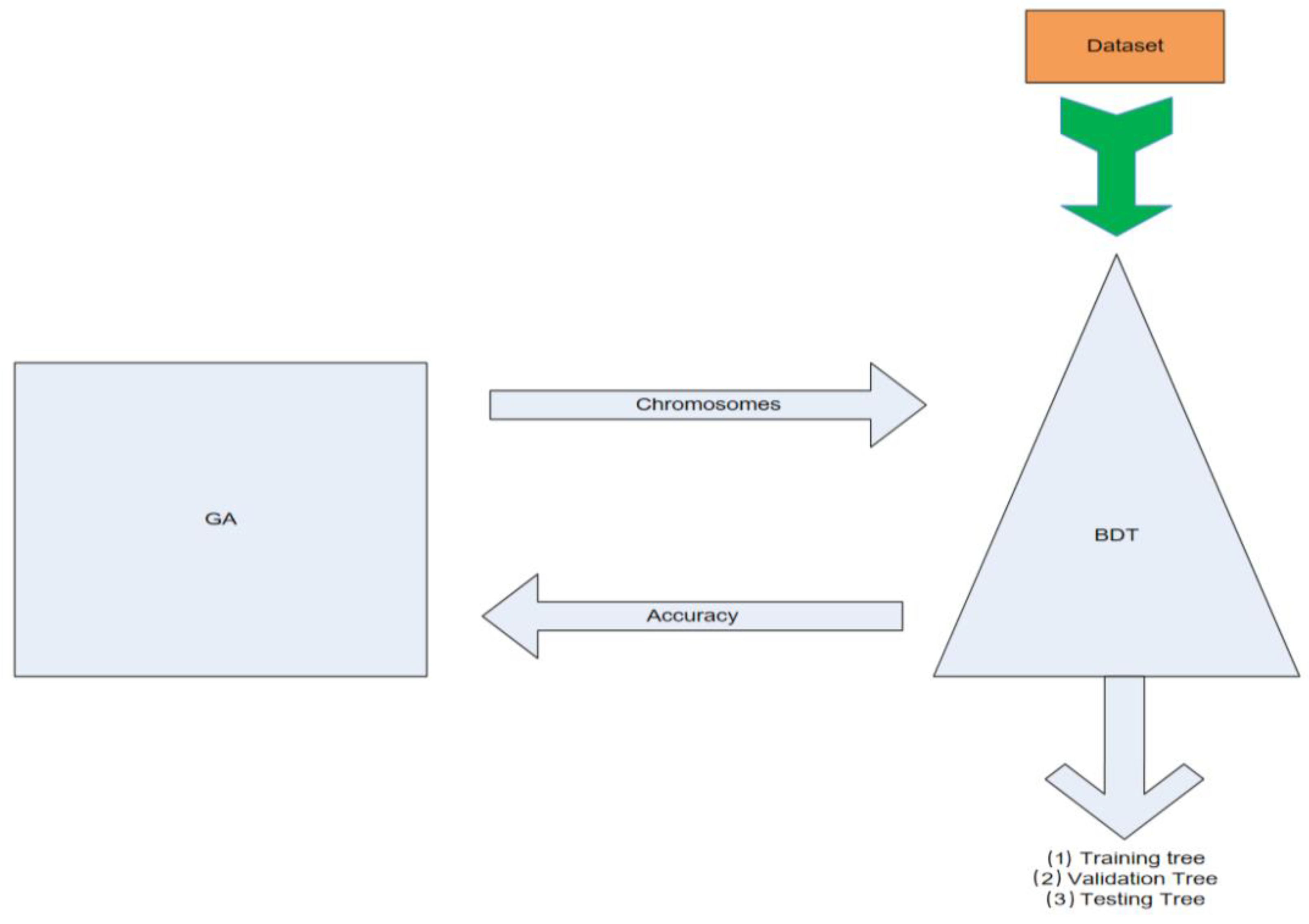
Figure 1. GA wrapper model. This figure demonstrates the overall wrapping classification and data exchange procedure of the binary decision trees and the genetic algorithm.
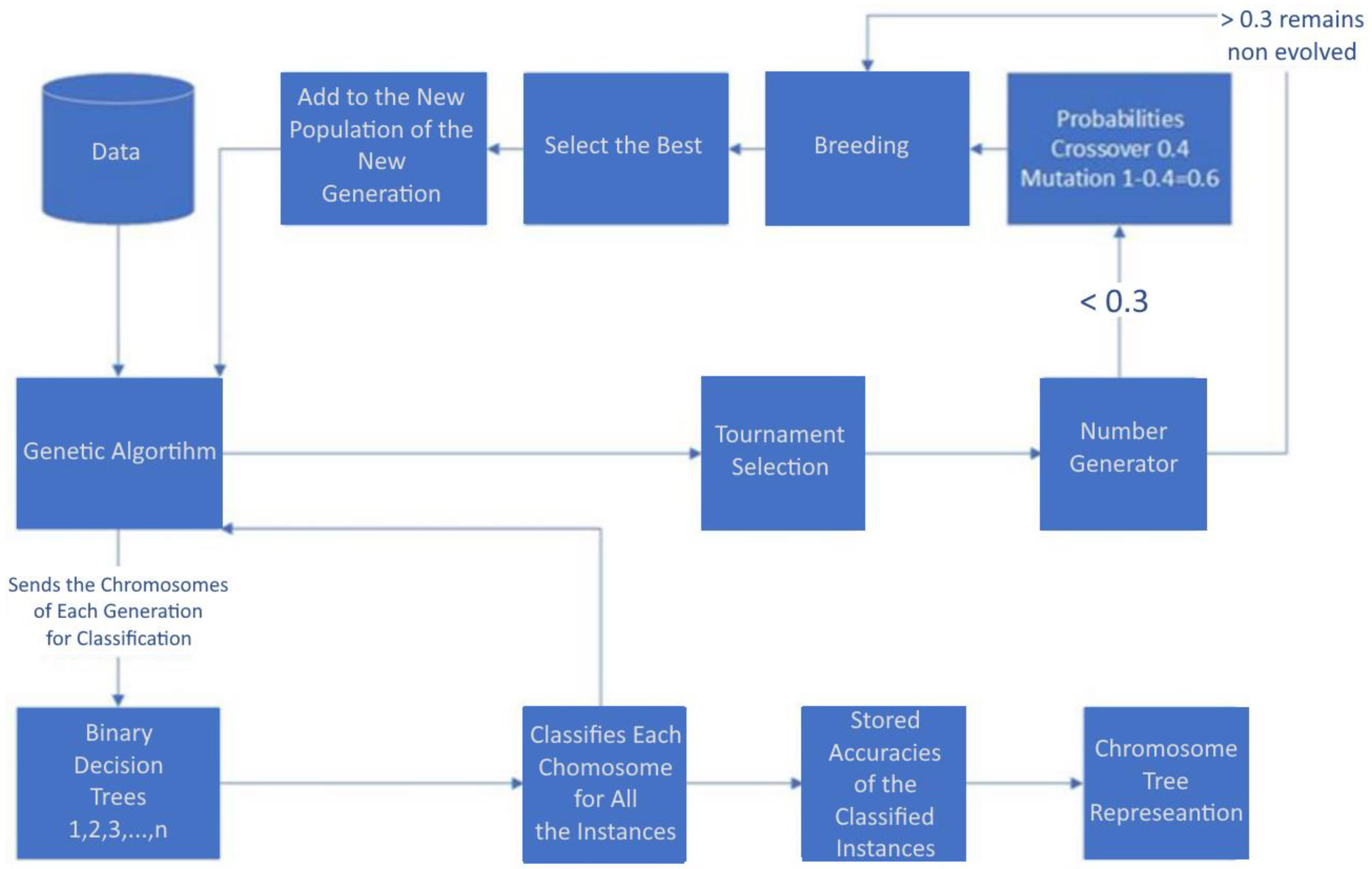
Informatics 10 00063 g001
Figure 2. Flowchart for the genetic algorithm wrapper.
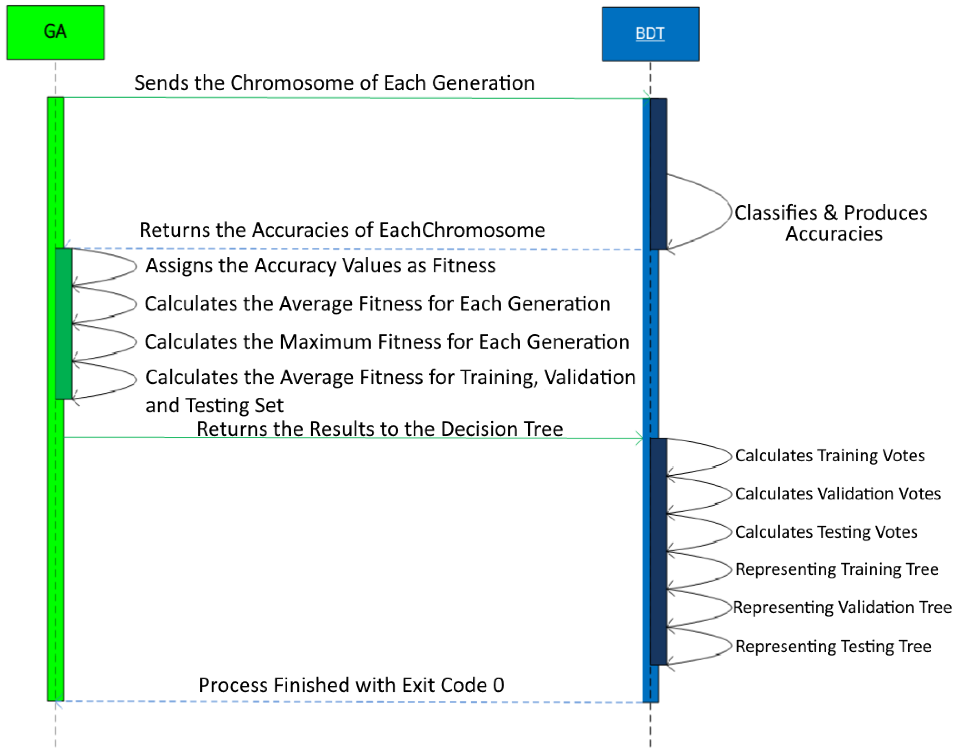
Informatics 10 00063 g002
Figure 3. Sequence diagram for binary decision tree and genetic algorithm communication.
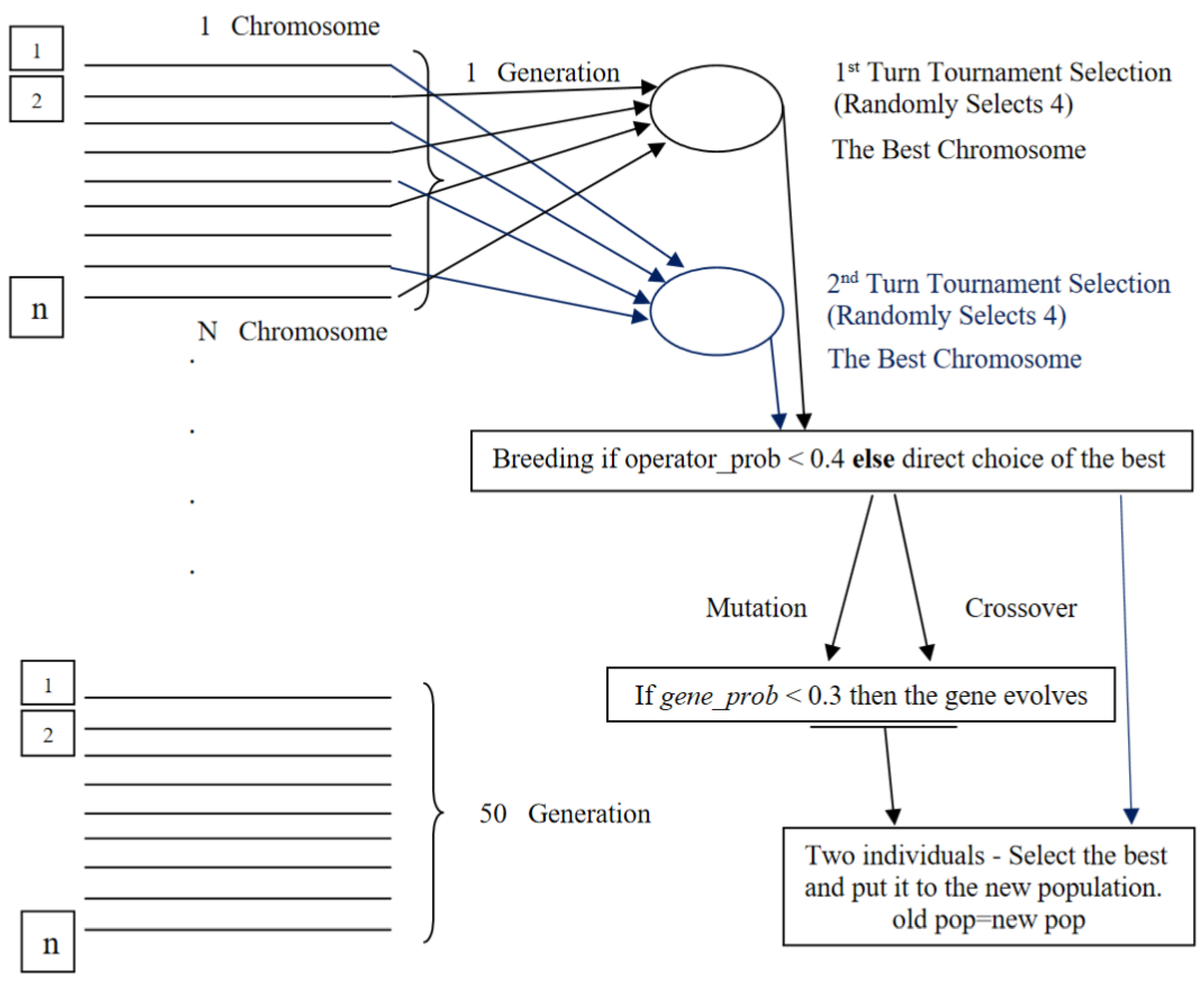
Informatics 10 00063 g003
Figure 4. Dataflow diagram for the GA Wrapper generic procedures.
Informatics 10 00063 g004
Figure 5. 
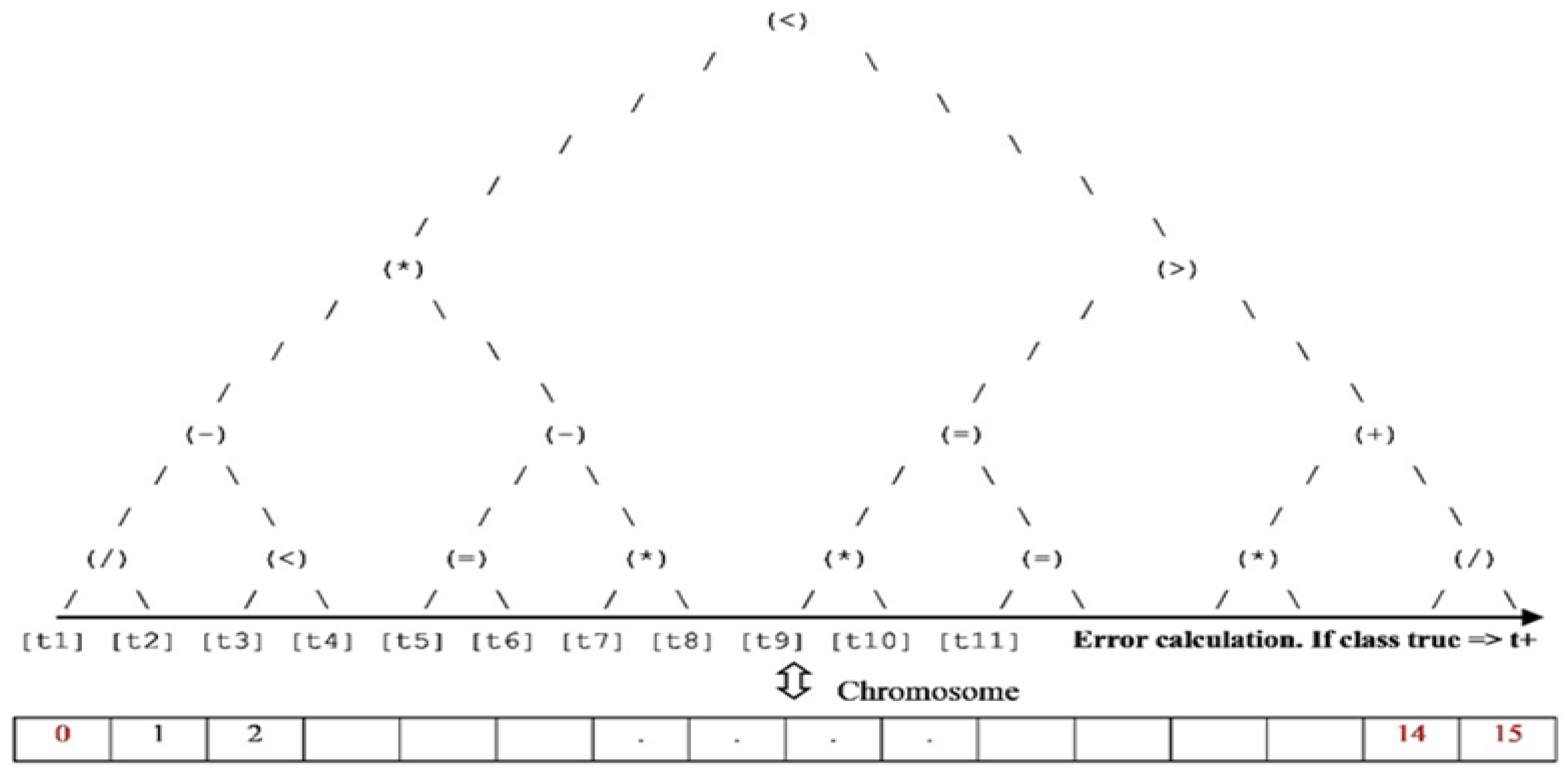
Optimal feature/chromosome representation. The gene positions are indicated with black color and the gene class numbers are indicated with red color.
Informatics 10 00063 g005
Figure 6. Best chromosome classification (7th run).
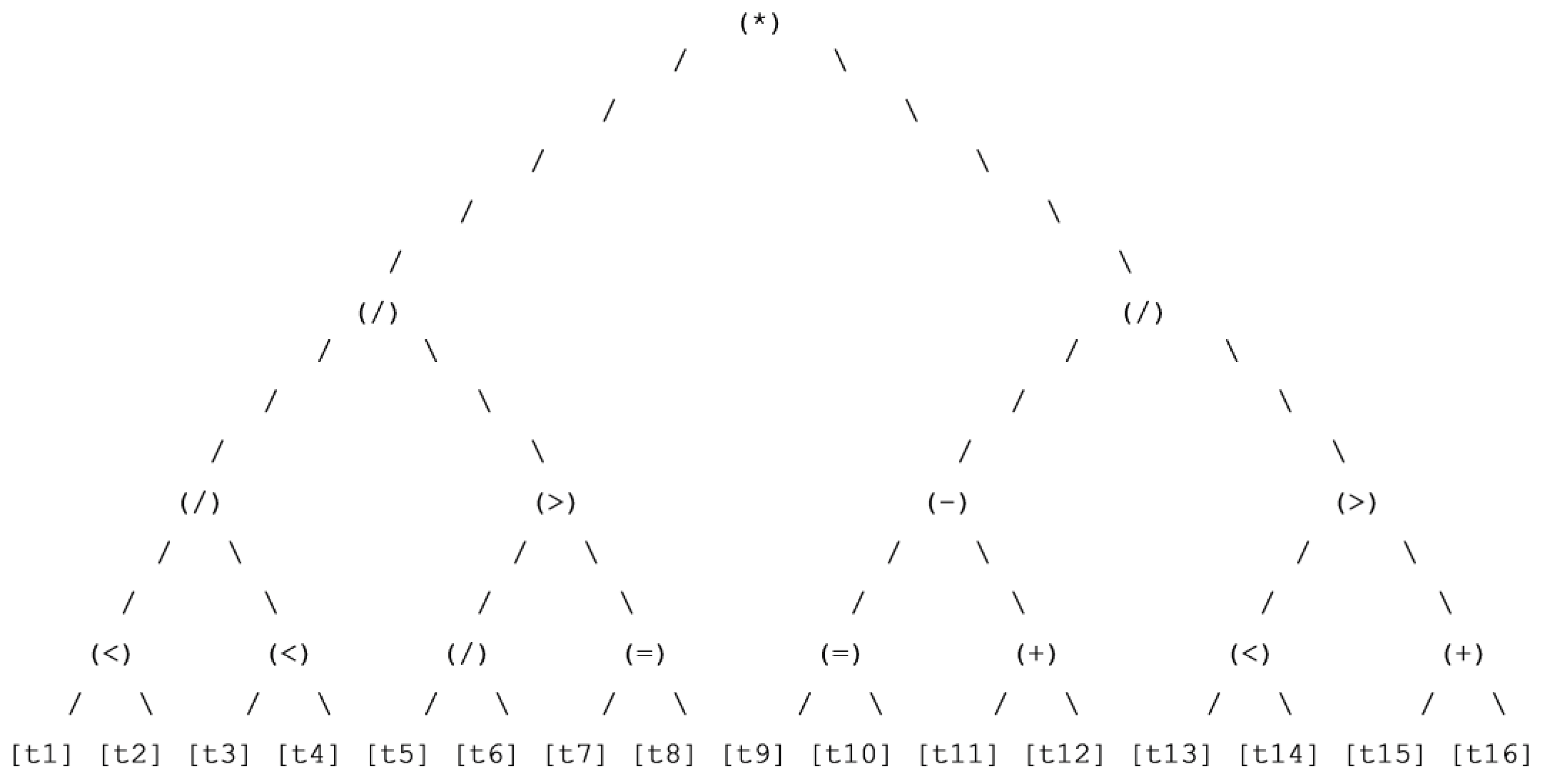
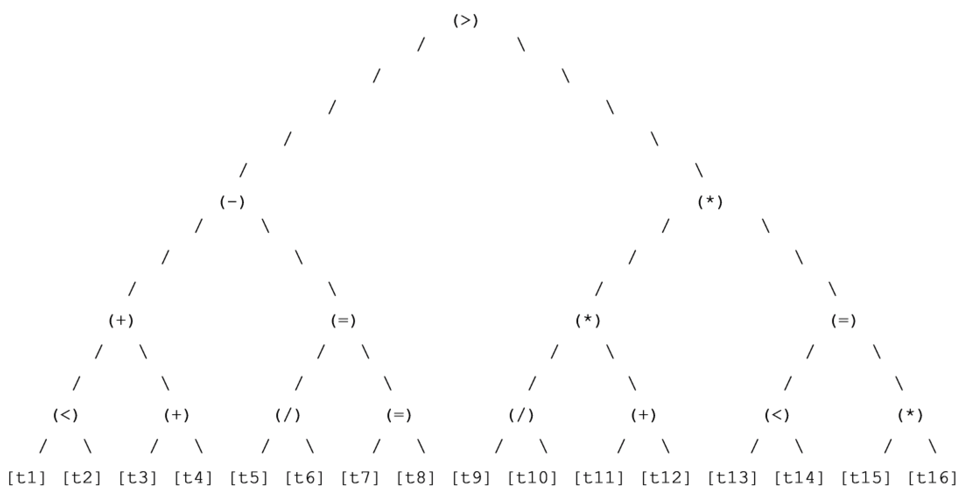
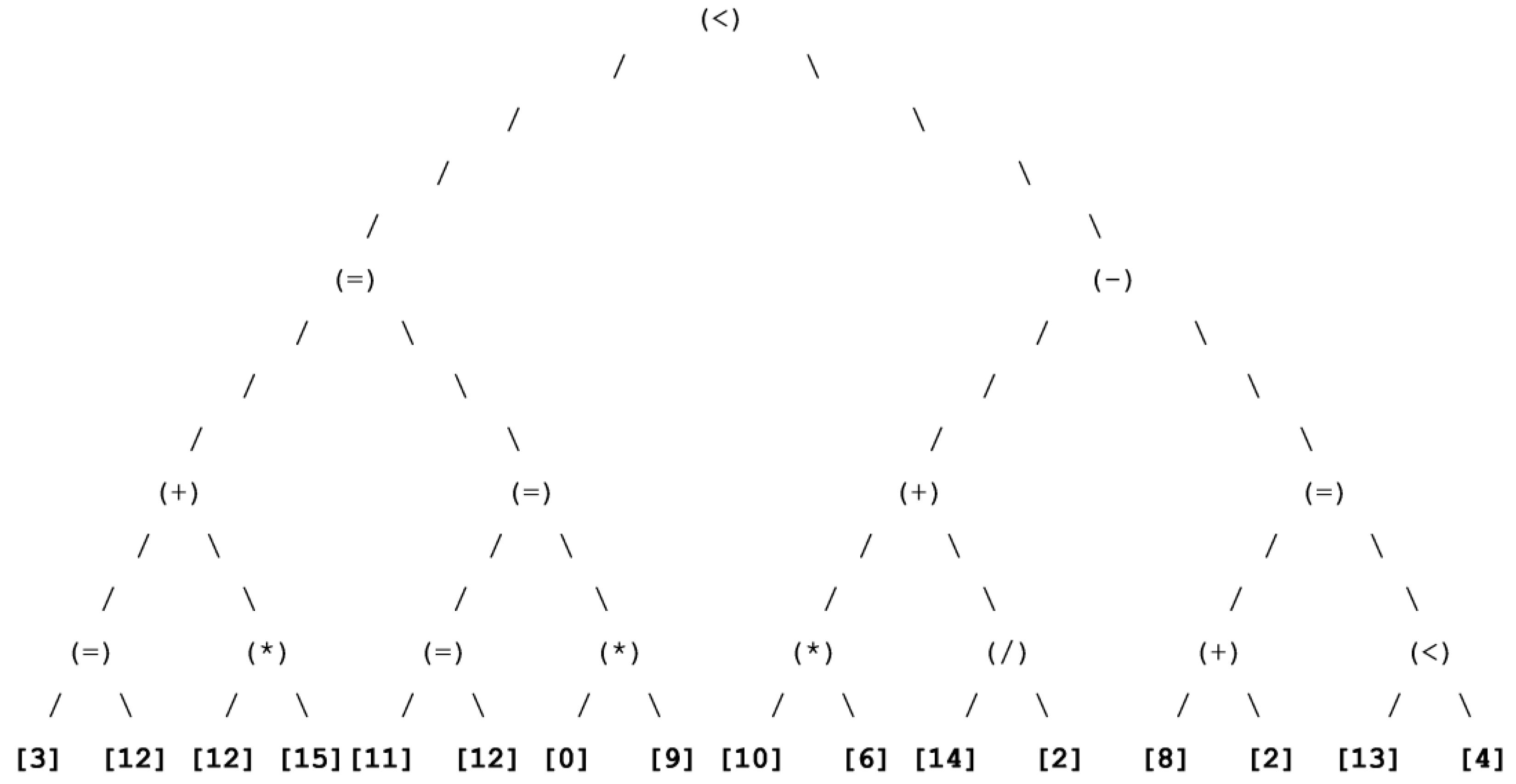
Informatics 10 00063 g006
Figure 7. 
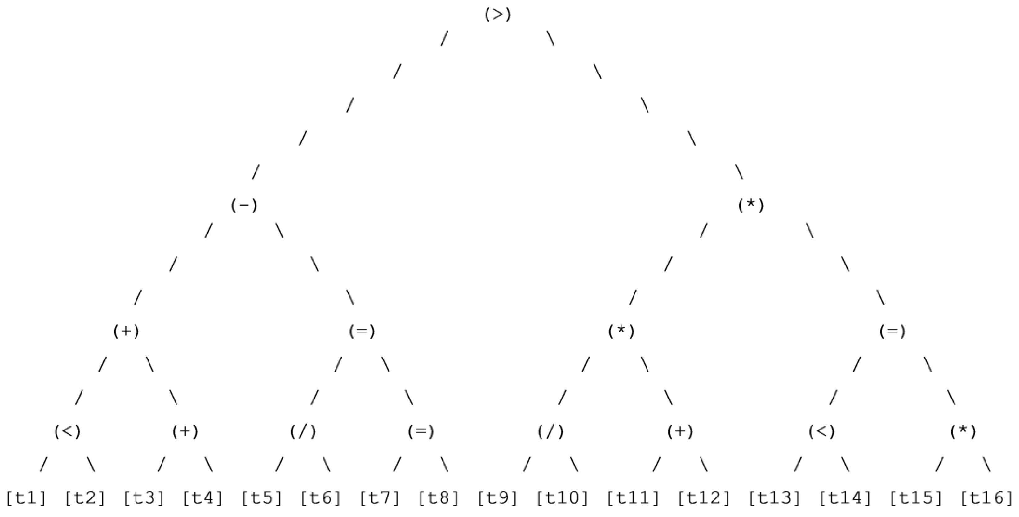
Dominant training BDT for wine classification.
Informatics 10 00063 g007
Figure 8. Dominant validation BDT for wine classification.
Informatics 10 00063 g008
Figure 9. Dominant testing BDT for wine classification.
Informatics 10 00063 g009
Figure 10. Best chromosome testing BDT for wine.
Informatics 10 00063 g010
Figure 11. 
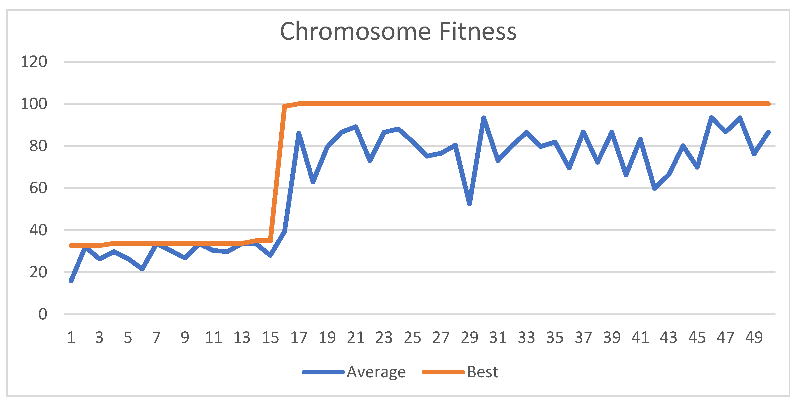
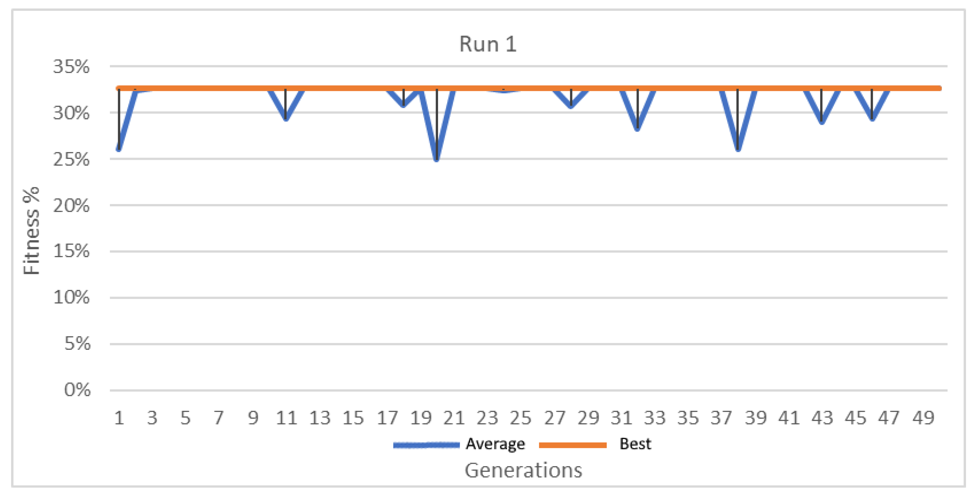
Best and average GA wrapper fitness run 1.
Informatics 10 00063 g011
Figure 12. 
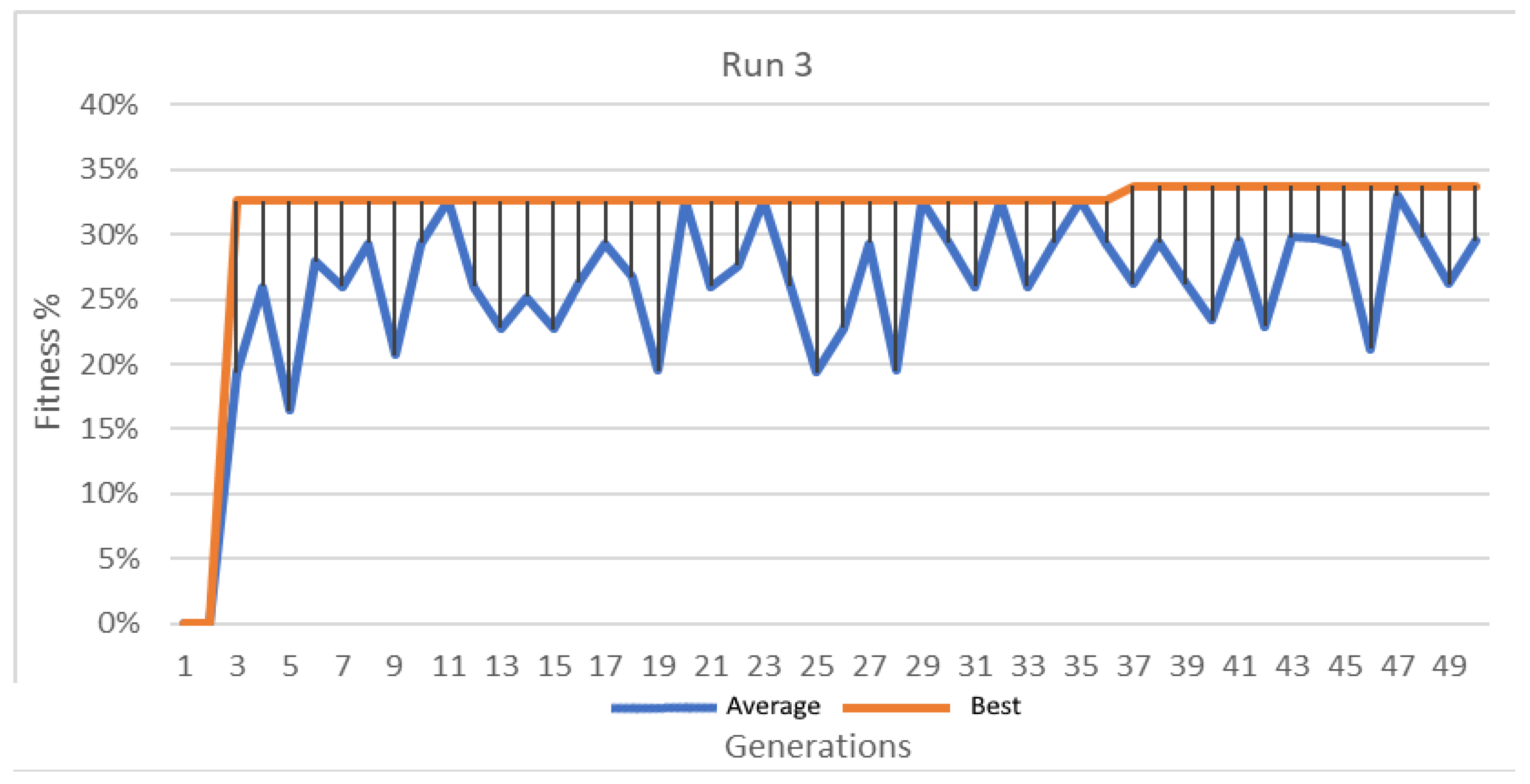
Best and average GA wrapper fitness run 3.
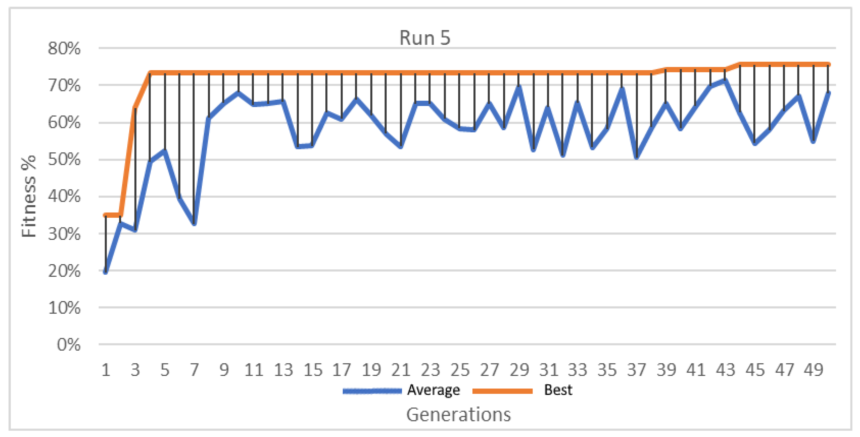
Informatics 10 00063 g012
Figure 13. Best and average GA wrapper fitness run 5.
Informatics 10 00063 g013
Figure 14. 
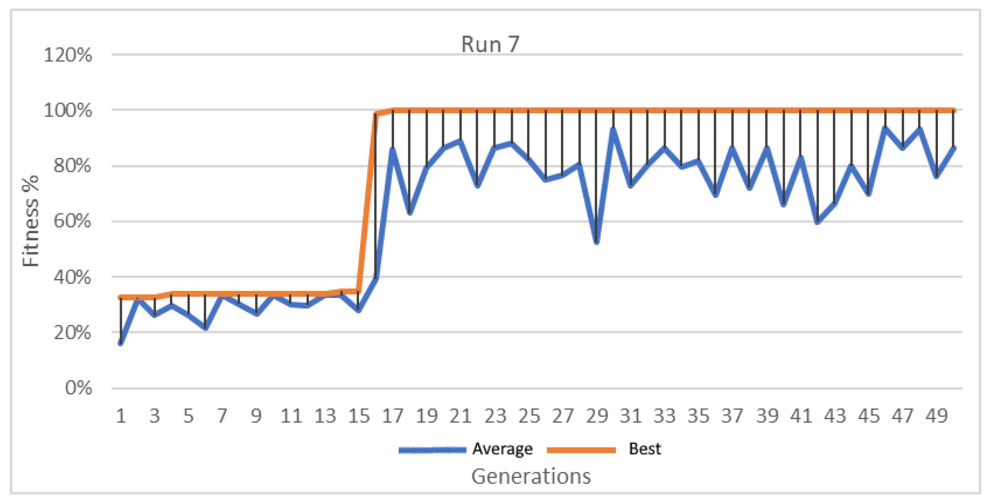
Best and average GA wrapper fitness run 7.
Informatics 10 00063 g014
Figure 15. 
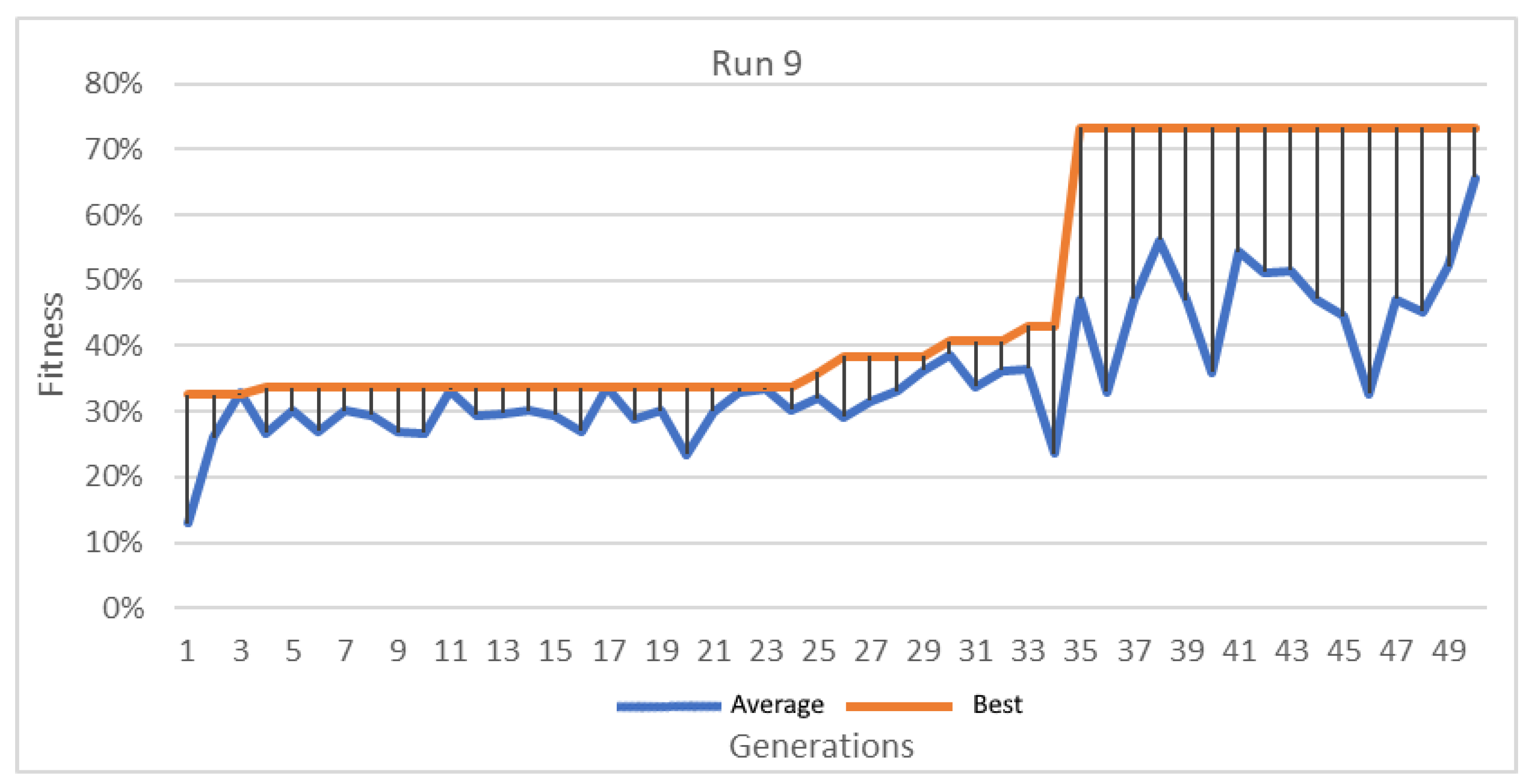
Best and average GA wrapper ritness run 9.
Informatics 10 00063 g015
Figure 16. 
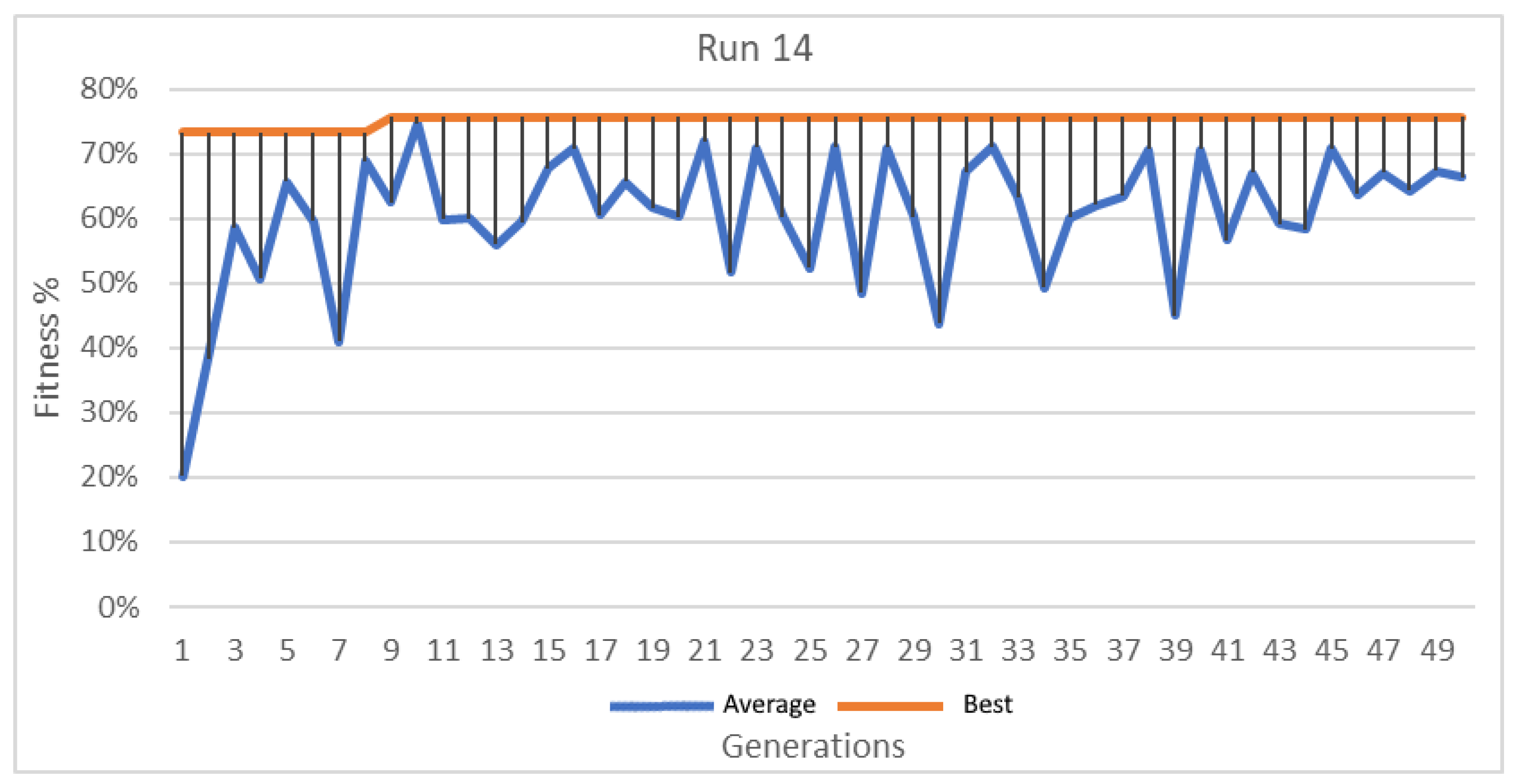
Best and average GA wrapper ritness run 14.
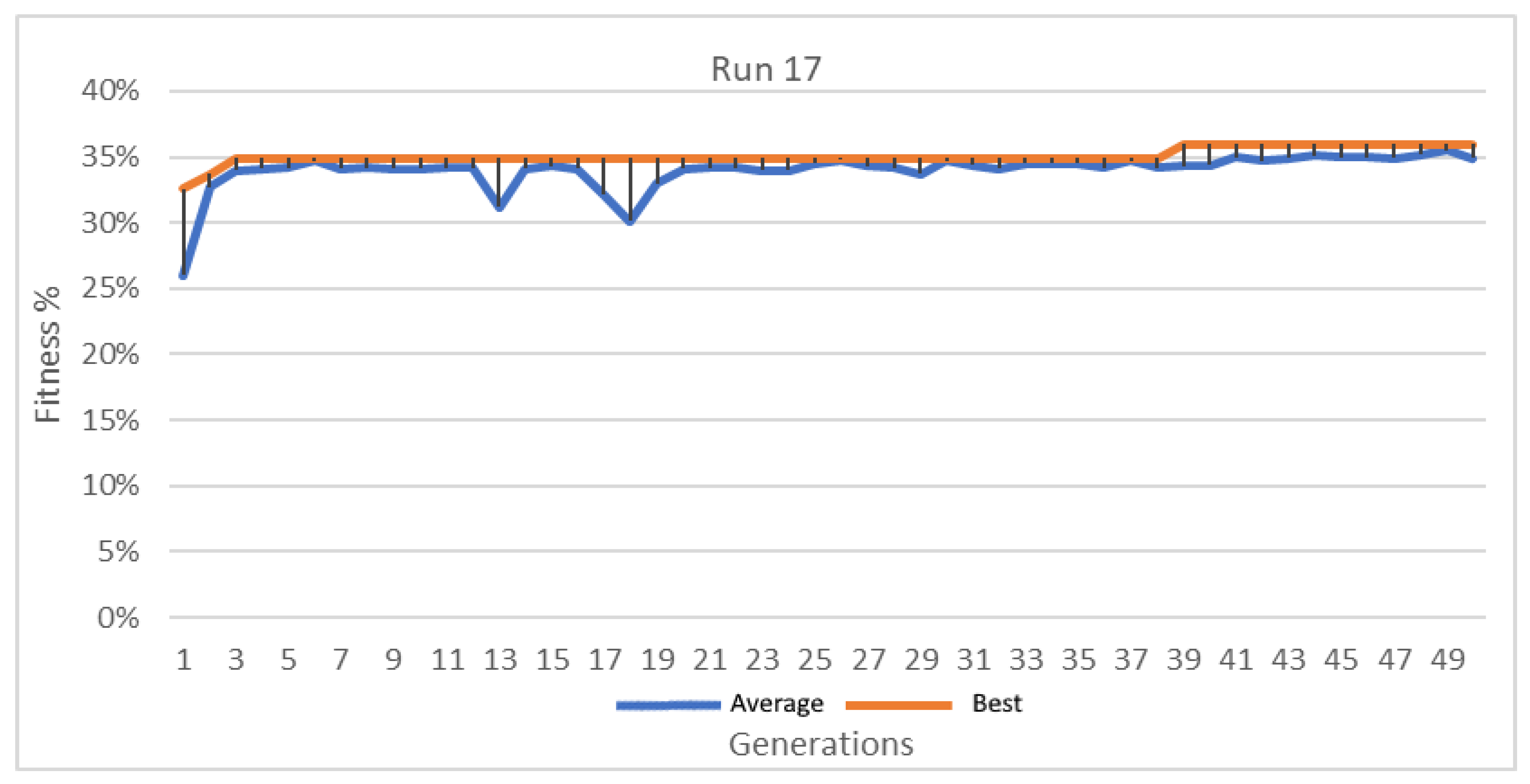
Informatics 10 00063 g016
Figure 17. Best and average GA wrapper fitness run 17.
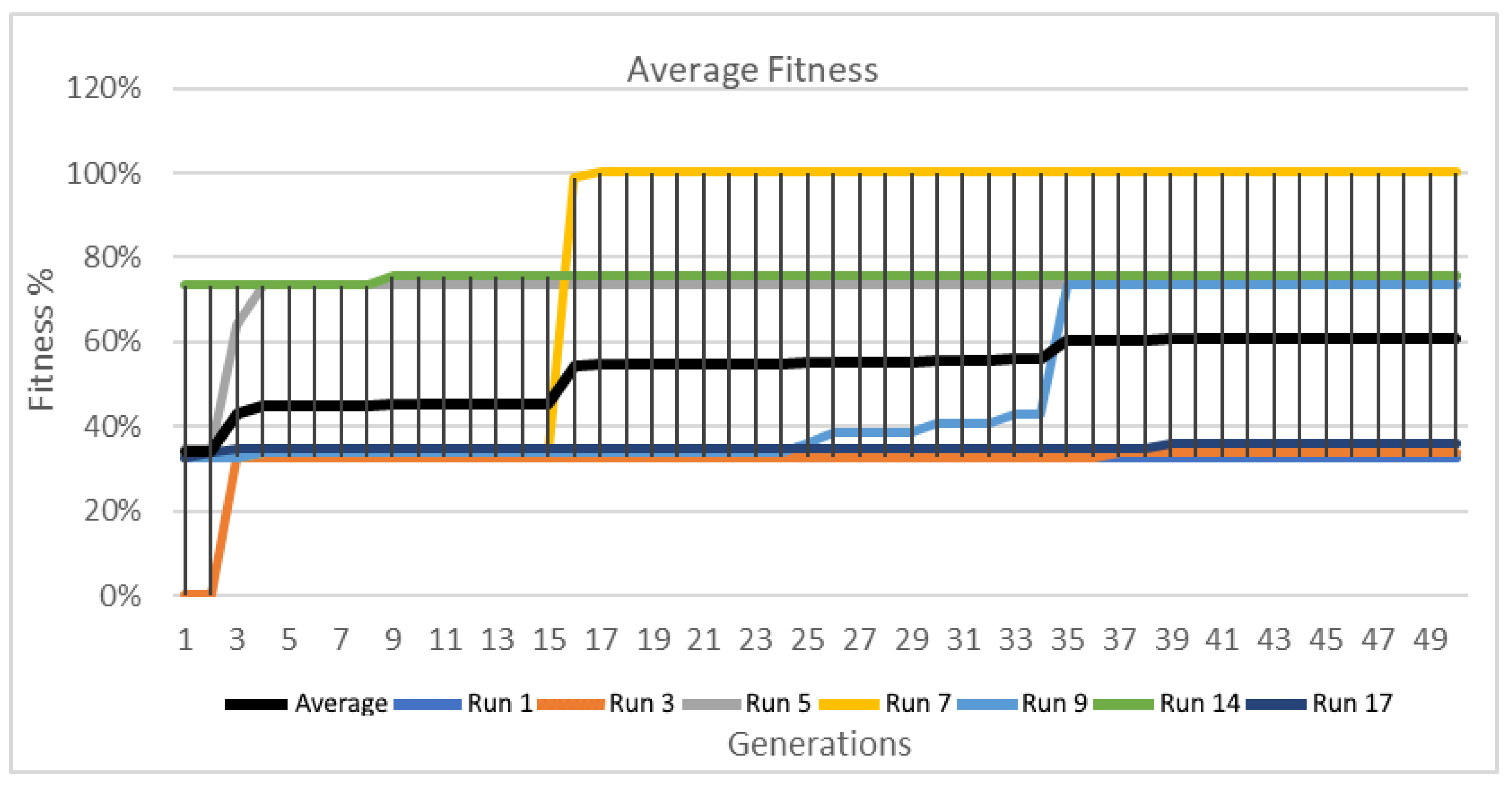
Informatics 10 00063 g017
Figure 18. GA wrapper average fitness.
Informatics 10 00063 g018
Figure 19. GA wrapper performance on wine data.
Informatics 10 00063 g019
Table 1. GA Wrapper Development Research Objectives.
NoResearch Objective (RO)Sub-Objectives
1GA Wrapper Model Design
  • Define the GA Wrapper Analysis
2.
Define The GA Wrapper Design
2GA Wrapper Model
Implementation
  • Genetic Algorithm Development
2.
Genetic Algorithm Training
3.
Genetic Algorithm Validation
4.
Genetic Algorithm Testing
5.
Genetic Algorithm Representation
3GA Wrapper Model
Performance
  • GA Wrapper on New Data
2.
Calculate Class Errors
3.
Calculate Generations Fitness
4.
Calculate Best Fitness
5.
Calculate Optimal BDTs
6.
Visualize Dominant BDTs
7.
Calculate Best Chromosome’s Gene Sequence
8.
Represent Generations’ Fitness Graphical
9.
Calculate and Represent Average Chromosome’s Gene Frequencies
10.
Generate Rules for Wine Cultivars
Table 2. Binary Decision Tree Pseudocode.
  • Function Decision_Tree(Atts,default,examples);
  • Atts ⟵ Attributes;
  • Default ⟵ default_typical_class;
  • Examples ⟵ Examples;
  • best_att ⟵ 0;
  • AttsValue[i] ⟵ Atts[1…N];
  • Subset[i] ⟵ 0;
  • subTree ⟵ 0;
  • Create Node StartNode;
  • If Examples have the same classification thendo
  • return classification;
  • If Examples is empty thendo
  • return Default classification;
    • best_Att ⟵ Find_best_Att(Atts,examples)
    • StartNode ⟵ best_att;
    • For any AttsV(i) of Atts do
    • Examples(i) ⟵ Best AttsValue[i] from Examples;
    • If subTree is not empty do
    • then
      • new_atts ⟵ atts-best_att;
      • subTree ⟵ create_Decision_Tree(subTree,new_atts);
      • attach subtree as child of StartNode;
    • else
      • create leaf node K;
      • K ⟵ default;
      • attach K as child of StartNode;
  • return StartNode;
Table 3. GA wrapper pseudocode.
//Cross-over probability ⟵ 40%
//Mutation Probability ⟵ 60%
//Tournament Selection ⟵ 4
//Gene Probability ⟵ 0.3
Init GA()
G ⟵ 100//Generations
P ⟵ 500//Population size
OP ⟵ 0.4//Operator probability
Init elitist[], parent[], offspring[], newPop[], pop[]
 
for g = 0 to G
  elitist = getTrainingElitist(pop)
  for b = 0 to P//Breeding loop
    for s = 0 to 2
      parent[s] ⟵ copy(select(pop))
    offspring ⟵ (getRandDouble() < OP)? crossOver(parent):mutate(parent)
    newPop[b] ⟵ (getTrainingFitness(offspring[0]) > getTrainingFitness(offspring[1]))? offspring[0]: offspring[1] 
 
  pop[getRandInt(P)] ⟵ elitist;
  pop ⟵ newPop;
Table 4. Wine dataset features.
FeaturesDescription
Title of DatabaseWine recognition data
Updated 21 September 1998 by C. Blake
Attribute13
Attributes ValuesContinuous
Missing Attribute ValuesNone
Class 159
Class 271
Class 348
Table 5. Wine dataset.
CultivarsGenes
Alcohol1st
Malic Acid2nd
Ash3rd
Alkalinity of Ash4th
Magnesium5th
Total Phenols6th
Flavonoids7th
Nonflavonoid Phenols8th
Proanthocyanins9th
Color Intensity10th
Hue11th
OD280/OD315 of Diluted Wines12th
Proline13th
Table 6. Best chromosome classification for the 7th run.
GeneGene OccurrenceClass
01Class[0] = 0.32558139534883723
Class[1] = 0.0
Class[2] = 0.0
32 Class [ 0 ] = 0.32558139534883723
Class [ 1 ] = 0.0
Class [ 2 ] = 7.946212766144101   ×   10 175
41 Class [ 0 ] = 0.32936722552731207
Class [ 1 ] = 5.936939424814535   ×   10 53
Class [ 2 ] = 9.23978228621407   ×   10 177
61 Class [ 0 ] = 0.0038298514596199077
Class [ 1 ] = 6.903417935830854   ×   10 55
Class [ 2 ] = 1.0743932890946594   ×   10 178
81 Class [ 0 ] = 4.453315650720823   ×   10 5
Class [ 1 ] = 8.027230157942853   ×   10 57
Class [ 2 ] = 1.2492945222030923   ×   10 180
91 Class [ 0 ] = 2.1585872418998667   ×   10 10
Class [ 1 ] = 1.3138540684740537   ×   10 33
Class [ 2 ] = 2.044778408520832   ×   10 157
101 Class [ 0 ] = 1.8563850280338853   ×   10 8
Class [ 1 ] = 1.1299144988876862   ×   10 31
Class [ 2 ] = 1.7585094313279154   ×   10 55
111 Class [ 0 ] = 1.5964911241091413   ×   10 6
Class [ 1 ] = 9.717264690434101   ×   10 30
Class [ 2 ] = 1.512318110942007   ×   10 153
121 Class [ 0 ] = 1.3729823667338616   ×   10 4
Class [ 1 ] = 8.356847633773327   ×   10 28
Class [ 2 ] = 1.3005935754101261   ×   10 151
131 Class [ 0 ] = 0.32558139534883723
Class [ 1 ] = 4.571263847550701   ×   10 20
Class [ 2 ] = 7.114352985929144   ×   10 144
143 Class [ 0 ] = 0.32936722552731207
Class [ 1 ] = 5.315423078547327   ×   10 22
Class [ 2 ] = 8.272503472010632   ×   10 146
151 Class [ 0 ] = 0.015457758436364094
Class [ 1 ] = 6.180724509938753   ×   10 24
Class [ 2 ] = 9.619190083733293   ×   10 148
Note: Numbers’ exponent of ten (E-###) are close to zero.
Table 7. Optimal decision trees for wine classification.
Training Votes Validation VotesTesting Votes
Tree[0] = 10,449Tree[0] = 3Tree[0] = 0
Tree[1] = 0Tree[1] = 0Tree[1] = 0
Tree[2] = 263,411Tree[2] = 225Tree[2] = 33 ⟵ max. no
Tree[3] = 1578Tree[3] = 0Tree[3] = 0
Tree[4] = 15,488Tree[4] = 0Tree[4] = 0
Tree[5] = 15,288Tree[5] = 0Tree[5] = 0
Tree[6] = 102,215Tree[6] = 184Tree[6] = 0
Tree[7] = 123,836Tree[7] = 38Tree[7] = 0
Tree[8] = 10,051Tree[8] = 0Tree[8] = 0
Tree[9] = 452,790 ⟵ max. no.Tree[9] = 264 ⟵ max. no.Tree[9] = 21
Table 8. Best chromosome gene frequency for class gender.
Gene PositionGene Name (Feature/Attribute)Gene VariablesOccurrences
0Class 1, Class 2, Class 3-1
1AlcoholReal0
2Malic AcidReal2
3AshReal1
4Alkalinity of AshReal1
5MagnesiumReal0
6Total PhenolsReal1
7FlavonoidsReal0
8Nonflavonoid PhenolsReal1
9ProanthocyaninsReal1
10Color IntensityReal1
11HueReal1
12OD280/OD315 of Diluted WinesReal3
13ProlineInteger1
14Additional Classes {1,2,3}-1
Table 9. 
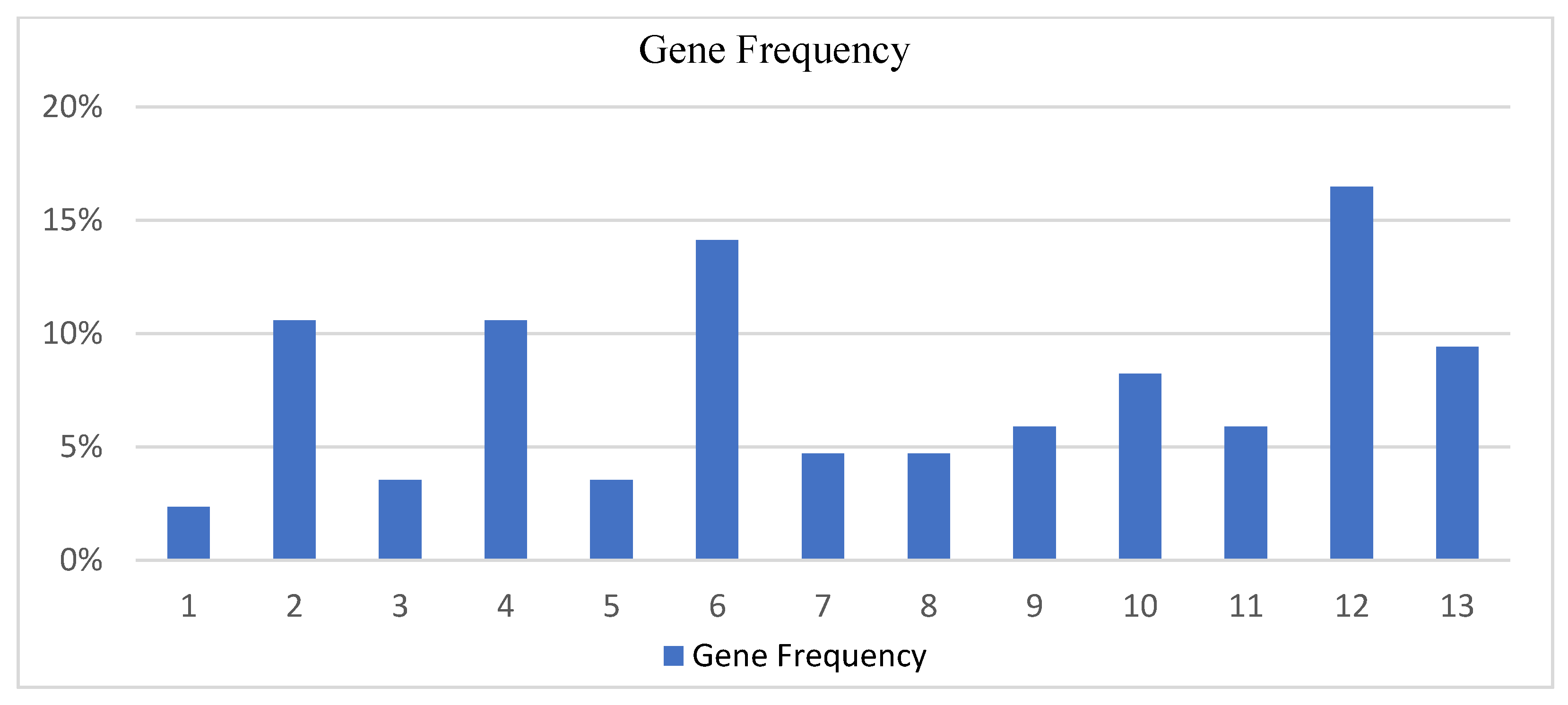
Average genes frequency from 7 runs for the wine origin dataset.
RunsGenes Average Frequency of Occurrence
Gene1st 2nd3rd4th 5th 6th 7thAvg. OccurrenceAvg. Occurrence %
101000100.2857142.35%
221103021.28571410.58%
300010110.4285713.52%
400121411.28571410.58%
500000300.4285713.52%
622401211.71428614.11%
711101000.5714294.70%
821000010.5714294.70%
911001110.7142865.88%
10112101118.23%
1102200010.7142865.88%
121204403216.47%
1310222011.1428579.41%
Disclaimer/Publisher’s Note: The statements, opinions and data contained in all publications are solely those of the individual author(s) and contributor(s) and not of MDPI and/or the editor(s). MDPI and/or the editor(s) disclaim responsibility for any injury to people or property resulting from any ideas, methods, instructions or products referred to in the content.

