Article

Optimal Surplus-Dependent Reinsurance under Regime-Switching in a Brownian Risk Model

by
Julia Eisenberg
1,*,
Lukas Fabrykowski
2 and
Maren Diane Schmeck
3
1
Department of Financial and Actuarial Mathematics, TU Wien, Wiedner Hauptstraße 8–10/E105-1, 1040 Vienna, Austria
2
Triangular IT Solutions e.U., 1220 Vienna, Austria
3
Center for Mathematical Economics, Bielefeld University, Universitätsstraße 25, 33615 Bielefeld, Germany
*
Author to whom correspondence should be addressed.
Risks 2021, 9(4), 73; https://doi.org/10.3390/risks9040073
Submission received: 10 February 2021 / Revised: 1 April 2021 / Accepted: 7 April 2021 / Published: 13 April 2021
(This article belongs to the Special Issue Interplay between Financial and Actuarial Mathematics)

Abstract

:
In this paper, we consider a company that wishes to determine the optimal reinsurance strategy minimising the total expected discounted amount of capital injections needed to prevent the ruin. The company’s surplus process is assumed to follow a Brownian motion with drift, and the reinsurance price is modelled by a continuous-time Markov chain with two states. The presence of regime-switching substantially complicates the optimal reinsurance problem, as the surplus-independent strategies turn out to be suboptimal. We develop a recursive approach that allows to represent a solution to the corresponding Hamilton–Jacobi–Bellman (HJB) equation and the corresponding reinsurance strategy as the unique limits of the sequence of solutions to ordinary differential equations and their first- and second-order derivatives. Via Ito’s formula, we prove the constructed function to be the value function. Two examples illustrate the recursive procedure along with a numerical approach yielding the direct solution to the HJB equation.

1. Introduction

Writing red numbers is generally considered a bad sign for the financial health of a (insurance) company. An old but also highly criticised concept to measure company’s riskiness is the ruin probability, i.e., the probability that the company’s surplus will become negative in finite time. There is a vast of literature on ruin probability in different settings and under various assumptions, see, for instance, Rolski et al. (1999); Asmussen and Albrecher (2010) and further reference therein.
As ruin probabilities do not take into account the time and the severity of ruin, the related concept of capital injections incorporating both features has been suggested in Pafumi (1998) in the discussion of Gerber and Shiu (1998). The risk is measured by the expected discounted amount of capital injections needed to keep the surplus non-negative. If the discounting rate, or rather the preference rate of the insurer, is positive, then the amount of capital injections is minimised if one injects just as much as it is necessary to shift the surplus to zero (but not above) and to inject just when the surplus becomes negative (but not before, anticipating a possible ruin), see, for instance, Eisenberg and Schmidli (2009).
A well-established way to reduce the risk of an insurance portfolio is to buy reinsurance. Finding the optimal or fair reinsurance in different settings is a popular and widely investigated topic in insurance mathematics, see, for instance, Azcue and Muler (2005); Ben Salah and Garrido (2018); Brachetta and Ceci (2020) and the references therein. However, the reinsurance premia are usually higher than the premia of the first insurer. Otherwise, it would create an arbitrage opportunity for the first insurer, who could transfer the entire risk to the reinsurer (i.e., the amount of the necessary capital injection is zero) and still receive a risk-free gain in from of the remaining premium payments. If we consider a model including both capital injections and reinsurance, the capital injection process will naturally depend on the chosen reinsurance strategy. That is, one can control the capital injections—representing the company’s riskiness—by reinsurance. In this context, the problem of finding a reinsurance strategy leading to a minimal possible value of expected discounted capital injections has been solved in Eisenberg and Schmidli (2009). There, the optimal reinsurance strategy is given by a constant, meaning that the insurance company is choosing a retention level once and forever. This result has been obtained under the assumption that the parameters describing the evolution of the insurer’s and reinsurer’s surplus never change. However, the reality offers a contrary picture. The state of economy has an enormous impact on the insurance/reinsurance companies, adding an exogeneously given source of uncertainty.
In financial literature, regime-switching models have become very popular because they take into account possible macroeconomic changes. Originally proposed by Hamilton to model stock returns, this class of models has been adopted also in insurance mathematics, see, e.g., Asmussen (1989); Bargès et al. (2013); Bäuerle and Kötter (2007); Gajek and Rudź (2020); Jiang and Pistorius (2012). In this connection, one should not forget the models containing hidden information. Reinsurance companies deciding over the price of their reinsurance products have to take into account the competition on the market and the consequences of adverse selection, see, for instance, Chiappori et al. (2006) and references therein.
In the present paper, we model the surplus of the first insurer by a Brownian motion with drift. The insurer is obligated to inject capital if the surplus becomes negative and is allowed to buy proportional reinsurance. In order to account for the macroeconomic changes that are assumed to happen in circles, we allow the price of the reinsurance—represented through a safety loading—to depend on the current regime of the economy. A continuous-time Markov chain with two states describes the length of the regimes and the switching intensity from one state into another. We target to find a reinsurance strategy that minimises the value of expected discounted capital injections where the discounting rate is a positive regime-independent constant. If the discounting rate would be assumed to be negative in one of the states, it might become optimal to inject capital even if the surplus is still positive (see, for instance, in Eisenberg and Krühner (2018)), which would substantially complicate the problem. For the same reason, we do not incorporate hidden information or moral hazard into this model
We solve the optimisation problem via the Hamilton–Jacobi–Bellman (HJB) equation, which is in this case a system of equations. Differently than it has been done in the one-regime case, we cannot guess the optimal strategy and prove the corresponding return function to solve the HJB equation. Instead, we solve the system of HJB equations recursively. First of all, the system of HJB equations is rewritten as a system of ordinary differential equations. Then, we assume that the value function, say in the second regime, is an exponential function and solve the corresponding ordinary differential equation for the first regime. The obtained solution is inserted into the ordinary differential equation for the second regime. Proceeding in this way, we obtain a monotone uniformly converging sequence of solutions, whose limit functions solve the original HJB equation. Here, it is of crucial importance to choose correctly the exponential of the starting function in the recursion. We present an equation system providing the only correct choice of the starting function.
The aim of the present paper is to develop an algorithm for finding a candidate for the value function. Like in the case with just one regime, the HJB equation is rewritten as a differential equation with boundary conditions. Here, we are facing a boundary value problem, i.e., the conditions are specified at different boundaries, with one boundary being even infinity. Therefore, using Volterra-type representations and comparison theorems, we prove the existence and uniqueness of a solution to the HJB equation. Ito’s formula allows one to show that the constructed solution is indeed the value function. We show that the optimal reinsurance strategies are increasing in one regime and decreasing in the other, depending on the parameters. This fact reflects the dependence of the strategies on the reinsurance prices along with the switching intensities. For instance, being in a regime with a low reinsurance price and a relative high switching intensity into a state with a high reinsurance price would produce a decreasing proportion of the self-insured risk.
As we do not get a closed form expressions for the value function and for the optimal strategies, we give a numerical illustration of both the algorithm and the value function. Here, we follow the approach of Auzinger et al. (2019).
The remainder of the paper is structured as follows. In Section 2, we give a mathematical formulation of the problem and present the Hamilton–Jacobi–Bellman equation. In Section 3, we shortly revise the case of constant controls and prove that those cannot be optimal except for the case when it is optimal to buy no reinsurance. In Section 4 and Section 5 we recursively construct a function solving the HJB equation and prove it to be the value function. Finally, we explore the problem numerically in Section 6 and conclude in Section 7.

2. The Model

In the following, we give a mathematical formulation of the problem and present the heuristically derived Hamilton–Jacobi–Bellman (HJB) equation. We are acting on a probability space ( Ω , F , P ) .
In the classical risk model, the surplus process of an insurance company is given by
X t = x + c t i = 1 N t Z i ,
where { N t } is a Poisson process with intensity λ and the claim sizes Z i are iid. with E [ Z 1 ] = μ and E [ Z 1 2 ] = μ 2 and independent of { N t } . Furthermore, x denotes the initial capital and c > 0 the premium rate. For further details on the classical risk model, see, e.g., Chapter 5.1 in Schmidli (2017).
The insurer can buy proportional reinsurance at a retention level 0 b 1 , i.e., for a claim Z i , the cedent pays b Z i , and the reinsurer pays the remaining claim ( 1 b ) Z i . Assume the expected value principle for the calculation of the insurance and reinsurance premia with safety loadings η > 0 and θ > 0 , respectively, where η < θ (see Chapter 1.10 in Schmidli (2017)) transforms the surplus of the insurer, denoted now by X b to
X b ( t ) = x + c ( b ) t i = 1 N t b Z i .
The new premium rate depends on the retention level and is given by c ( b ) = ( b ( 1 + θ ) ( θ η ) ) λ μ , being old premia reduced for the premia paid to the reinsurer (see, e.g., Chapter 5.7 in Schmidli (2017)).
Usually, optimisation problems can be tackled more easily if the surplus is given by a Brownian motion. Therefore, diffusion approximation of the classical risk model is a popular concept in optimisation problems in insurance. A diffusion approximation to (1) by adopting a dynamic reinsurance strategy B = { b t } , that is, the retention level b t changes continuously in time, is given by
X t B = x + θ 0 t b s d s λ μ ( θ η ) t + λ μ 2 0 t b s d W s ,
dfsuch that the first two moments of (1) and (2) remain the same; see, for instance, Appendix D.3 in Schmidli (2008) for details. In addition to buying reinsurance, the insurance company has to inject capital in order to keep the surplus non-negative. The process describing the accumulated capital injections up to time t under a reinsurance strategy B will be denoted by Y B = { Y t B } . The surplus process under a reinsurance strategy B and capital injections Y is given by
X t B , Y = X t B + Y t .
Further, we introduce a continuous-time Markov chain J = { J t } with state space S = { 1 , 2 } . We assume that J and W are independent, and that J has a strongly irreducible generator Q = [ q i j ] 2 × 2 , where q i j = q i i for i j , and we consider the filtration { F t } , generated by the pair ( W , J ) . That is, the economy can be in two different regimes, and accordingly the parameters in (2) are no longer constant, but depend on the state. In order to emphasise the dependence on the reinsurance price, we let the safety coefficient of the reinsurer depend on the current regime by letting all other variables unchanged. Thus, instead of (2), we now consider the process
X t B = x + 0 t θ J s b s λ μ ( θ J s η ) d s + 0 t λ μ 2 b s d W s ,
The set of admissible reinsurance strategies will be denoted by B and is formally defined as
B = { B = { b t } , b t [ 0 , 1 ] , b t F t adapted } .
We are interested in the minimal value of expected discounted capital injections by starting in state i with initial capital x over all admissible strategies, i.e., we minimise
V B ( i , x ) : = E i , x 0 e δ t d Y t B , ( i , x ) { 1 , 2 } × [ 0 , ) .
Here, and in the following, we use the common notation E [ . | X 0 = x , J 0 = i ] = E i , x [ . ] .
Our target is to find an admissible reinsurance strategy B such that the value function
V ( i , x ) : = inf B B V B ( i , x ) .
can be written as the return function corresponding to the strategy B , i.e., V ( i , x ) = V B ( i , x ) .
According to the theory of stochastic control, we expect the value function V is to solve the HJB equation (see Schmidli (2008) or Jiang and Pistorius (2012) for a model with Markov-switching)
inf b [ 0 , 1 ] λ μ 2 b 2 2 V ( i , x ) + λ μ θ i b θ i + η V ( i , x ) ( δ q i i ) V ( i , x ) q i i V ( j , x ) = 0 ,
The boundary condition V ( i , 0 ) = 1 arises from the requirement of smooth fit ( C 1 -fit) at zero. As we do not allow the surplus to become negative, it is clear that the value function for x < 0 fulfils V ( i , x ) = x + V ( i , 0 ) , i.e., we immediately inject as much capital as it is needed to shift the surplus process to zero, meaning V ( i , x ) = 1 . The second boundary condition lim x V ( i , x ) = 0 originates from the fact that a Brownian motion with a positive drift converges to infinity almost surely, i.e., for x the amount of expected discounted capital injections converges to 0, see, for instance, Rolski et al. (1999).
The HJB equation can be formally derived as the infinitesimal version of the dynamic programming principle, upon assuming that V has the regularity needed to apply Ito’s formula for Markov-modulated diffusion processes (as in the proof of Lemma 1 below); we refer to Chapter 2 in Schmidli (2008) for a textbook treatment.
It is clear that b ( i , x ) = μ θ i V ( i , x ) μ 2 V ( i , x ) 1 . If b < 1 , the HJB becomes for i , j { 1 , 2 } i j
μ 2 θ i 2 V ( i , x ) 2 2 μ 2 V ( i , x ) λ μ θ i η V ( i , x ) ( δ q i i ) V ( i , x ) q i i V ( j , x ) = 0 .
Technically, HJB Equation (5) is a system of 2 ordinary differential equations, coupled through the transition rates of the underlying Markov chain. It is a hard task to explicitly solve these equations and show that the solutions are decreasing and convex functions of the initial capital. Therefore, we use a recursive method to obtain the value function as a limit. However, first we look at the constant strategies and investigate why none of those can be optimal in the case of more than one regime.

3. Constant Strategies

It is known (see, for instance, Eisenberg and Schmidli (2009)) that in the one-regime case the optimal reinsurance strategy is given by a constant. In this section, we show that in the two-regime case a constant strategy (other than “no reinsurance at all”) cannot be optimal.
Let b 1 , b 2 [ 0 , 1 ) , then B ^ : = { b J t } is an admissible reinsurance strategy. Further, we let Y ^ and X ^ denote the capital injection process triggered by the reinsurance strategy B ^ and the surplus process under B ^ and after capital injections, respectively. Thus, for the return function V ^ ( i , x ) , corresponding to B ^ , it holds
V ^ ( i , x ) = E i , x 0 e δ t d Y ^ t .
Lemma 1.
If u ^ is a solution to the system of ODEs, i { 1 , 2 } , j i
λ μ 2 b i 2 2 u ^ ( i , x ) + λ μ ( θ i b i θ i + η ) u ^ ( i , x ) ( δ q i i ) u ^ ( i , x ) q i i u ^ ( j , x ) = 0 ,
with boundary conditions u ^ ( i , 0 ) = 1 , lim x u ^ ( i , x ) = 0 , then u ^ ( i , x ) = V ^ ( i , x ) .
Proof. 
First, we look at the Equation (6). A general solution to (6) fulfilling lim x u ^ ( i , x ) = 0 is given by
u ^ ( i , x ) = C i 1 e A 1 x + C i 2 e A 2 x , i { 1 , 2 } ,
where A 1 , A 2 < 0 . The coefficients are uniquely given by
C 11 A 1 2 λ μ 2 b 1 2 2 + A 1 λ μ ( θ 1 b 1 θ 1 + η ) ( δ q 11 ) q 11 C 21 = 0 , C 12 A 2 2 λ μ 2 b 1 2 2 + A 2 λ μ ( θ 1 b 1 θ 1 + η ) ( δ q 11 ) q 11 C 22 = 0 , C 21 A 1 2 λ μ 2 b 2 2 2 + A 1 λ μ ( θ 2 b 2 θ 2 + η ) ( δ q 22 ) q 22 C 11 = 0 , C 22 A 2 2 λ μ 2 b 2 2 2 + A 2 λ μ ( θ 2 b 2 θ 2 + η ) ( δ q 22 ) q 22 C 12 = 0 , C 11 A 1 + C 12 A 2 = 1 , C 21 A 1 + C 22 A 2 = 1 .
Now, arguing like in Shreve et al. (1984), we show that u ^ = V ^ . Using a generalised form of Itô’s formula, like it has been done, for instance, in Jiang and Pistorius (2012), we get
e δ t u ^ ( J t , X ^ t ) = u ^ ( J 0 , X ^ 0 ) + 0 t e δ s u ^ ( J s , X ^ s ) d W s + M t + 0 t e δ s { λ μ 2 b s 2 2 u ^ ( J s , X ^ s ) + λ μ ( θ J s b s θ J s + η ) u ^ ( J s , X ^ s ) ( δ q J s , J s ) u ^ ( J s , X ^ s ) q J s , J s u ^ 1 1 [ J s = 1 ] + 1 , X ^ s } d s + 0 t e δ s u ^ ( J s , X ^ s ) d Y ^ s
where M is a local martingale associated with the regime switching mechanism. That is, M is given by
M t = [ 0 , t ] × [ 0 , 2 ] u ^ ( X ^ s , j ) u ^ ( X ^ s , J s ) π ˜ ( d s , d j ) ,
where π ˜ = π ν is a compensated random measure as defined in Jacod and Shiryaev (2003). It holds
π ( d t , d j ) = s 0 1 1 [ Δ J s ( ω ) 0 ] 1 1 ( d t , d j ) ( s , J s ( ω ) ) , ν ( d t , d j ) = 1 1 [ Δ J t ( ω ) 0 ] q J t , j P ( d j ) d t ,
where P is the counting measure on { 1 , 2 } and 1 1 ( d t , d j ) ( s , J s ( ω ) ) is the Dirac measure at the point ( s , J s ( ω ) ) .
Note that M is bounded because
| u ^ ( j , X ^ s ) u ^ ( J s , X ^ s ) | max i { 1 , 2 } u ^ ( i , X ^ s ) ,
As u ^ is bounded, we can conclude that M is a martingale with expectation zero. Because u ^ is bounded we can conclude that also the stochastic integral is a martingale with expectation zero. Further, as u ^ solves Equation (6) with u ( i , 0 ) = 1 , building expectations on the both sides in (9) yields
E e δ t u ^ ( J t , X ^ t ) = u ^ ( i , x ) E 0 t e δ s d Y ^ s .
By the bounded convergence theorem, we can interchange limit t and expectations and get u ^ ( i , x ) = E 0 e δ s d Y ^ s .    □
Remark 1.
Note that it holds C i j 0 for all i , j { 1 , 2 } . If, for example, C 11 = 0 then we have from (8) that it must also hold C 21 = 0 and simultaneously
C 22 = 1 A 2 = C 12 , C 22 A 2 2 λ μ 2 b 1 2 2 + A 2 λ μ ( θ 1 b 1 θ 1 + η ) ( δ q 11 ) q 11 = 0 , C 22 A 2 2 λ μ 2 b 2 2 2 + A 2 λ μ ( θ 2 b 2 θ 2 + η ) ( δ q 22 ) q 22 = 0 ,
which leads to a contradiction.
Lemma 2.
The return function corresponding to a strategy B = { b J s } with b i [ 0 , 1 ) , i = 1 , 2 , does not solve HJB Equation (4).
Proof. 
We proof this lemma by contradiction. Assume that there is a strategy B = { b J s } with b i [ 0 , 1 ) , i = 1 , 2 , so that the corresponding return function, V ^ solves the HJB Equation (4), i.e.,
0 = inf b [ 0 , 1 ] λ μ 2 b 2 2 V ^ ( i , x ) + λ μ ( θ i b θ i + η ) V ^ ( i , x ) ( δ q i i ) V ^ ( i , x ) q i i V ^ ( j , x ) .
Subtracting Equation (6) from the latter, one finds
0 = inf b [ 0 , 1 ] λ μ 2 b 2 2 V ^ ( i , x ) + λ μ ( θ i b θ i + η ) V ^ ( i , x ) ( δ q i i ) V ^ ( i , x ) q i i V ^ ( j , x ) λ μ 2 b ^ i 2 2 V ^ ( i , x ) + λ μ ( θ i b ^ i θ i + η ) V ^ ( i , x ) ( δ q i i ) V ^ ( i , x ) q i i V ^ ( j , x ) ,
which is equivalent to
λ μ 2 b ^ 2 2 V ^ ( i , x ) + λ μ θ i b ^ i V ^ ( i , x ) = inf b [ 0 , 1 ] λ μ 2 b 2 2 V ^ ( i , x ) + λ μ θ i b i V ^ ( i , x ) .
Then, it should hold that b i = μ θ i μ 2 V ^ ( i , x ) V ^ ( i , x ) 1 . As we assumed b ^ i < 1 , for i = 1 , 2 , the expression μ θ i μ 2 V ^ ( i , x ) V ^ ( i , x ) should not depend on x. Keeping in mind the boundary conditions lim x V ^ ( i , x ) = 0 and V ( i , 0 ) = 1 , we get
V ^ ( i , x ) = e μ θ i μ 2 b ^ i x ,
which contradicts (7).    □

4. Recursion

In the following, we establish an algorithm that allows us to calculate the value function as a limit of a sequence of twice continuously differentiable, decreasing and convex functions. For simplicity, we let
Δ i : = λ μ 2 θ i 2 2 μ 2 + δ q i , B i : = Δ i λ μ ( θ i η ) , B ˜ i : = Δ i + q i λ μ ( θ i η ) .
We will see that the behaviour of the optimal reinsurance strategy will depend on the relations between B 1 , B ˜ 1 , B 2 and B ˜ 2 . As there are many possibilities to arrange the above quantities, we consider just one path, omitting considering the case of no reinsurance, in order not to complicate the explanations. However, the algorithm proposed below can be applied to any combination of parameters.
Assumption 1.
W.l.o.g. we assume that B 1 > B ˜ 1 > B 2 > B ˜ 2 > max { μ θ 2 μ 2 , μ θ 1 μ 2 } , which is equivalent to
1 B 1 < 1 B ˜ 1 < 1 B 2 < 1 B ˜ 2 < max μ 2 μ θ 2 , μ 2 μ θ 1 .
In the case of just one regime, the problem could be solved by conjecturing that the optimal strategy is constant and the corresponding return function is an exponential function. This allowed us to verify easily that the solution, say v, to Differential Equation (5) with q i i = 0 was strictly increasing, convex and fulfilled μ θ i v μ 2 v < 1 or, if the case maybe, the optimal strategy was not to buy reinsurance at all. In our case of two regimes, the situation changes as we have seen in Section 3. The return functions corresponding to the constant strategies do not solve the HJB equation in general.
As it is impossible to guess the optimal strategy and to subsequently check whether the return function corresponding to this strategy is the value function, we slightly change the solving procedure. At first, we look at the HJB equation in the form of Differential Equation (5), such has been done, for instance, in Eisenberg and Schmidli (2009). The next, very technical step is to solve the obtained differential equation and to check whether the solution, say f, fulfils μ θ i f ( i , x ) μ 2 f ( i , x ) ( 0 , 1 ) . Then, we show that the gained solution f is indeed the return function corresponding to the reinsurance strategy μ θ i f ( i , x ) μ 2 f ( i , x ) ( 0 , 1 ) . Thus, in this way we find an admissible strategy whose return function solves HJB Equation (4). Verification theorem proves this return function to be the value function.
In the following, we describe the steps of an algorithm allowing to get a strictly decreasing and convex solution to Differential Equation (5) under Assumption (11). The procedure consists in choosing a starting function, fixing, say i = 1 , and replacing the unknown function V ( 2 , x ) in (5) by the chosen starting function. Using the method of Højgaard and Taksar (1998), we show the existence and uniqueness of a solution. In the next step, now it holds i = 2 , the unknown function V ( 1 , x ) in (5) is replaced by the function obtained in the first step. Letting the number of steps go to infinity, we get a solution to (5). We will see that the starting value of the recursion plays a crucial role in obtaining a solution with the desired properties: convexity and monotonicity. Therefore, we start by explaining how to choose the starting function in Step 0.

4.1. Step 0

The solutions to the differential equations
λ μ 2 θ i 2 f ( x ) 2 μ 2 f ( x ) λ μ θ i η f ( x ) δ f ( x ) = 0 .
with boundary conditions lim x f ( x ) = 0 and f ( 0 ) = 1 are well known and given by 1 B ˜ i e B ˜ i x . Note that due to Assumption (11) it holds that μ θ i μ 2 B ˜ i < 1 .
The optimal strategy in the case of two regimes is not constant, see Section 3. However, we conjecture that the value function in the case of two regimes fulfils lim x V ( 1 , x ) V ( 1 , x ) = lim x V ( 2 , x ) V ( 2 , x ) [ 1 / B ˜ 1 , 1 / B ˜ 2 ] , i.e., the ratio of the first and second derivatives converges to the same value does not matter the initial regime state. One can see it as a sort of averaging of the optimal strategies from the one-regime cases. This means, for instance, that if in one-regime case the optimal reinsurance level was low in the first state and high in the second, in the two-regime case the optimal level in the first state will go up and go down in the second.
Mathematically, the above explanations are reflected in the starting function of our algorithm:
W 0 ( x ) : = 1 Λ e Λ x ,
where Λ fulfils
λ μ ( θ 1 η ) B 1 Λ 1 + q 11 Λ e α = 0 , λ μ ( θ 2 η ) B 2 Λ 1 + q 22 Λ e α = 0 .
It means that Λ and α are uniquely given by
Λ = B 1 + B 2 D 2 and α = ln B 1 B 2 + D 2 q 11 / λ μ ( θ 1 η ) , D : = ( B 1 B 2 ) 2 + 4 q 11 q 22 λ 2 μ 2 ( θ 1 η ) ( θ 2 η ) .
Remark 2.
It is a straightforward calculation to show Λ ( B ˜ 2 , B ˜ 1 ) and α > 0 using the definition of B i and Assumption (11).
Note that due to our assumption, it holds that μ θ i W 0 ( x ) μ 2 W 0 ( x ) < 1 .
We will see by establishing the algorithm below that Equation (14) for Λ will be crucial in order to obtain a well-defined solution to (5). The elaborated mathematical meaning and explanation of the Equation (14) will be demonstrated in the following steps.

4.2. Step 1

Assuming (11), we start investigating Differential Equation (5) and substitute the term q 11 V ( 2 , x ) by q 11 W 0 ( x ) defined in (13), i.e., we look now at the differential equation
λ μ 2 θ 1 2 f ( x ) 2 μ 2 f ( x ) λ μ θ 1 η f ( x ) ( δ q 11 ) f ( x ) q 11 W 0 ( x ) = 0 .
Although we know the function W 0 , differential Equation (16) still cannot be solved in a way that we could easily prove the solution to be strictly decreasing and convex. Therefore, we use the following technique, introduced in Højgaard and Taksar (1998).
We assume that there is a strictly increasing, bijective on R + function g such that the derivative of the solution f to (16) fulfils f ( g ( x ) ) = e x . Then, it holds
f ( g ( x ) ) = e x g ( x ) and f ( g ( x ) ) = e x g ( x ) 2 e x g ( x ) 3 .
Differentiating (16) yields
λ μ 2 θ 1 2 2 μ 2 2 f ( x ) f ( x ) 2 f ( x ) ( f ( x ) ) 2 θ 1 η f ( x ) ( δ q 11 ) f ( x ) q 11 W 0 ( x ) = 0 .
Changing the variable to g ( x ) leads to a new differential equation for the function g
λ μ 2 θ 1 2 2 μ 2 2 e x + e 3 x ( g ( x ) ) 2 1 + g ( x ) g ( x ) e 2 x / ( g ( x ) ) 2 λ μ θ 1 η e x g ( x ) + ( δ q 11 ) e x q 11 W 0 ( g ( x ) ) = 0 ,
which can be further simplified by multiplying by e x g ( x ) and inserting the definition of  B 1 :
λ μ 2 θ 1 2 2 μ 2 g ( x ) = λ μ ( θ 1 η ) g ( x ) B 1 1 + q 11 g ( x ) e Λ g ( x ) + x .
As the function g should be bijective, we will prove the existence and uniqueness of a solution to (17) on R + with the boundary conditions guaranteeing g ( R + ) = R + and g > 0 . In particular, the term e Λ g ( x ) + x determines the unique condition yielding g > 0 and lim x g ( x ) , namely, lim x g ( x ) = 1 / Λ .
In order to guide the reader through the auxiliary results below, we provide a roadmap identifying the key findings of Step 1.
Note that when investigating (17) we are looking at a boundary value problem. To show the existence and uniqueness of a solution, we will translate the boundary value problem into an initial value problem, i.e., we shift the condition g ( x ) 1 / Λ as x to x = 0 by using Volterra type representation for (17).
  • First, we show that if (17) has a solution, say g, with the boundary values g ( 0 ) = 0 and g ( n ) = 1 / Λ , for some n N , then g ( 0 ) 1 / B ˜ 1 , 1 / Λ .
  • In the second step, we show that there is a unique solution ξ n to (17) with the boundary conditions ξ n ( 0 ) = 0 and ξ n ( n ) = 1 / Λ .
  • We prove the existence of a solution g 1 to (17) with g ( 0 ) = 0 and lim x g 1 ( x ) = 1 / Λ .
  • It holds g 1 ( 0 ) ( 1 / B ˜ 1 , 1 / Λ ) and g 1 ( x ) > 0 .
  • The inverse function h 1 of g 1 fulfils h 1 ( Λ , B ˜ 1 ) and h 1 ( x ) < 0 .
  • h 1 ( x ) ( Λ x , B ˜ 1 x ) for all x > 0 and lim x h 1 ( x ) Λ x = α with α given in (15).
Lemma 3.
If there is a solution g to (17) with the boundary conditions g ( 0 ) = 0 , g ( n ) = 1 / Λ , for some n 1 , then it holds that
g ( 0 ) 1 / B ˜ 1 , 1 / Λ .
Proof. 
We prove the claim by contradiction. Let g be a solution to (17) with the boundary conditions g ( 0 ) = 0 , g ( n ) = 1 / Λ .
  • Assume for the moment that g ( 0 ) 1 / B ˜ 1 . Then,
    λ μ 2 θ 1 2 2 μ 2 g ( 0 ) = λ μ θ 1 η ( g ( 0 ) B ˜ 1 1 ) < 0 : if g ( 0 ) < 1 / B ˜ 1 , λ μ 2 θ 1 2 2 μ 2 g ( 0 ) = q 11 g ( 0 ) ( g ( 0 ) Λ + 1 ) < 0 : if g ( 0 ) = 1 / B ˜ 1 ,
    meaning that g ( x ) stays positive but below 1 / B ˜ 1 in an environment of 0. As B ˜ 1 > Λ , the function e Λ g ( x ) + x is increasing in an ε -environment of 0, i.e., e Λ g ( x ) + x > 1 , which means that
    λ μ 2 θ 1 2 2 μ 2 g ( x ) = ( g ( x ) B 1 1 ) λ μ θ 1 η + q 11 g ( x ) e Λ g ( x ) + x < ( g ( x ) B ˜ 1 1 ) λ μ θ 1 η < 0 .
    Thus, g will stay negative and g will never arrive at 1 / Λ > 1 / B ˜ 1 .
  • On the other hand, if g ( 0 ) 1 / Λ > 1 / B ˜ 1 , then in a similar way one concludes that g stays above 1 / Λ for all x ( 0 , n ] , contradicting g ( n ) = 1 / Λ .
  • Thus, we can conclude that g ( 0 ) 1 / B ˜ 1 , 1 / Λ .
   □
Lemma 4.
For every n 1 there is a unique solution ξ n ( x ) to (17) on [ 0 , n ] fulfilling ξ n ( 0 ) = 0 , ξ n ( n ) = 1 / Λ .
Proof. 
As the proof is very technical, we postpone it to Appendix A.    □
Lemma 5.
Let ξ n be the unique solution to (17) with the boundary conditions ξ n ( 0 ) = 0 and ξ n ( n ) = 1 / Λ . Then, ξ n ( x ) > 0 on [ 0 , ) .
Proof. 
See Appendix A.    □
Proposition 1.
There exists a unique solution g 1 to (17) with the boundary conditions g 1 ( 0 ) = 0 and lim x g 1 ( x ) = 1 / Λ , g 1 ( 1 / B ˜ 1 , 1 / Λ ) and g 1 > 0 on ( 0 , ) .
Proof. 
See Appendix A.    □
Remark 3.
Proposition 1 implies Λ g 1 ( x ) + x > 0 for all x > 0 . Moreover, due to Equation (14), it holds that
lim x ( Λ g 1 ( x ) + x ) = α .
where α is given in (15).
Note that the definition of g yields g ( x ) = f ( g ( x ) ) f ( g ( x ) ) . The boundary conditions imply lim x g ( x ) = and lim x g ( x ) = 0 . Thus, letting x in (17) and using (18), we get the first equation in (14). This provides the first idea and the meaning of the choice of  W 0 .
Corollary 1.
There is a strictly increasing and concave inverse function of g 1 on R + : g 1 1 ( x ) = : h 1 ( x ) . Further, it holds
  • h 1 fulfils h 1 ( x ) > 0 , h 1 ( Λ , B ˜ 1 ) , lim x h 1 ( x ) = Λ and h 1 ( x ) < 0 .
  • h 1 ( x ) Λ = 1 g ˜ 1 ( h 1 ( x ) ) Λ > 0 , i.e., h 1 ( x ) Λ x is strictly increasing with h 1 ( x ) > Λ x for x > 0 .
Proof. 
The function g 1 fulfils g 1 ( R + ) = R + and g 1 ( x ) > 0 for all x R + , i.e., g 1 is a bijective function, which implies the existence of an inverse function h 1 . All other properties follow from the properties of g 1 .    □
We can now let
W 1 ( x ) = x e h 1 ( y ) d y ,
i.e., W 1 ( x ) = e h 1 ( x ) . Note that W 1 is well defined due to Corollary 1 and solves Differential Equation (17) with the boundary conditions W 1 ( 0 ) = 1 and lim x W 1 ( x ) = 0 . In particular, due to (11) it holds μ θ 1 W 1 μ 2 W 1 < 1 .
In the following second step, we construct in a similar way a function g 2 .

4.3. Step 2

In the second step, we add the term q 22 g ( x ) W 1 ( g ( x ) ) e x to Differential Equation (12), i.e., we are looking at the differential equation
λ μ 2 θ 2 2 2 μ 2 g ( x ) = λ μ θ 2 η ( g ( x ) B 2 1 ) q 22 g ( x ) W 1 ( g ( x ) ) e x = λ μ θ 2 η ( g ( x ) B 2 1 ) + q 22 g ( x ) e h 1 ( g ( x ) ) + x .
Note that h 1 ( x ) C , which implies Lipschitz-continuity on compacts. The existence of a solution g 2 with the boundary conditions g 2 ( 0 ) = 0 and lim x g 2 ( x ) = 1 / Λ can be shown similar to Step 1.
The main findings of Step 2 are as follows:
  • There is a unique solution g 2 to (20) with the boundary conditions g 2 ( 0 ) = 0 and lim x g 2 ( x ) = 1 / Λ .
  • It holds that g 2 ( 0 ) ( 1 / Λ , 1 / B ˜ 2 ) and g 2 ( x ) < 0 .
  • The inverse function h 2 of g 2 fulfils h 2 ( B ˜ 2 , Λ ) and h 2 ( x ) > 0 .
  • h 2 ( x ) ( B ˜ 2 x , Λ x ) for all x > 0 .
In the following, we prove only the results that cannot be easily transferred from Step 1.
Lemma 6.
If there is a solution g 2 to Differential Equation (20) with the boundary conditions g 2 ( 0 ) = 0 and lim x g 2 ( x ) = 1 / Λ then g 2 ( 0 ) ( 1 / Λ , 1 / B ˜ 2 ) .
Proof. 
See Appendix A.    □
Lemma 7.
Let g 2 be the unique solution to Differential Equation (20) with the boundary conditions g 2 ( 0 ) = 0 and lim x g 2 ( x ) = 1 / Λ . Then, g 2 ( x ) < 0 for all x ( 0 , ) .
Proof. 
Lemma 6 yields g 2 ( 0 ) ( 1 / Λ , 1 / B ˜ 2 ) . It means (see (A1)) that g 2 ( 0 ) < 0 . Let x ^ : = inf { x > 0 : g 2 ( x ) = 0 } , then g 2 ( x ^ ) ( 1 / Λ , 1 / B ˜ 2 ) because if g 2 ( x ) = 1 / Λ and g 2 ( x ) < 0 then Lemma 6 gives lim x g 2 ( x ) 1 / Λ . Further, we also have
g 2 ( x ^ ) = q 22 g 2 ( x ^ ) g 2 ( x ^ ) h 1 ( g 2 ( x ^ ) ) + 1 e h 1 ( g 2 ( x ^ ) ) + x ^ > 0
because h 1 > Λ due to Corollary 1. Then, g 2 becomes positive, i.e., g 2 becomes increasing and stays increasing for g 2 > 1 / Λ , i.e., bounded away from 1 / Λ , which yields a contradiction.    □
Corollary 2.
Let h 2 ( x ) be the inverse function of g 2 ( x ) . Then, h 2 ( B ˜ 2 , Λ ) , h 2 > 0 , lim x h 2 ( x ) = Λ , h 2 ( x ) ( B ˜ 2 x , Λ x ) .
Proof. 
The proof is a direct consequence of Lemma 7.    □
Remark 4.
  • Let
    β : = lim x ( h 1 ( g 2 ( x ) ) + x ) .
    Then, due to Equation (14) it holds β = α .
  • Furthermore, it follows easily
    β = lim x ( h 1 ( g 2 ( x ) ) + x ) = lim x h 1 ( g 2 ( h 2 ( x ) ) ) + h 2 ( x ) = lim x h 1 ( x ) + Λ x Λ x + h 2 ( x ) ,
    and using (18) we get lim x ( h 1 ( x ) + Λ x ) = lim x ( x + Λ g 1 ( x ) ) = α .
    Therefore, we conclude
    lim x Λ x + h 2 ( x ) = β + α = 0
    as h 2 ( x ) Λ x , see Corollary 2
Remark 4 explains the second equation in (14), if we let x in Differential Equation (20).

4.4. Step 2m+1

In this step, we are searching for the function h 2 m + 1 as the inverse of the solution g 2 m + 1 to the differential equation U m ( g ) = 0 , where
U m ( g ) : = λ μ 2 θ 1 2 2 μ 2 g ( x ) λ μ θ 1 η ( g ( x ) B 1 1 ) q 11 g ( x ) e h 2 m ( g ( x ) ) + x .
The existence of a solution g 2 m + 1 can be proven similarly to Step 1. The boundary conditions are g 2 m + 1 ( 0 ) = 0 and lim x g 2 m + 1 ( x ) = 1 / Λ .
Our main target is to show that the obtained sequences of functions ( g 2 m + 1 ) , ( g 2 m + 1 ) and ( h 2 m + 1 ) are monotone. We carry out the proof by induction using as the induction step h 2 ( x ) < Λ x on ( 0 , ) , see Corollary 2 in Step 2.
The main findings of Step 2 m + 1 are summarised in the following remark.
Remark 5.
Similar to Step 1, we get for g 2 m + 1 and its inverse function h 2 m + 1 that
  • g 2 m + 1 ( 0 ) = h 2 m + 1 ( 0 ) = 0 ;
  • g 2 m + 1 ( 1 / B ˜ 1 , 1 / Λ ) , h 2 m + 1 ( Λ , B ˜ 1 ) ;
  • g 2 m + 1 ( x ) > 0 and h 2 m + 1 ( x ) < 0 ; and
  • lim x g 2 m + 1 ( x ) = 1 / Λ , lim x h 2 m + 1 ( x ) = Λ .
In Lemma 8 we show
  • g 2 m + 1 > g 2 m 1 on R + , g 2 m + 1 > g 2 m 1 and h 2 m + 1 < h 2 m 1 on ( 0 , ) .
Lemma 8.
Assume that the functions h 2 k obtained in Steps 2 k , 0 k m , fulfil
1.
h 2 k ( R + ) = R + , h 2 k ( 0 ) = 0 , h 2 k ( B ˜ 2 , Λ ) , h 2 k ( x ) Λ x , lim x h 2 k = Λ and h 2 k ( x ) > 0 , and
2.
h 2 k ( x ) < h 2 k 2 ( x ) for x > 0 .
Then, g 2 m + 1 > g 2 m 1 on R + , g 2 m + 1 > g 2 m 1 and h 2 m + 1 < h 2 m 1 on ( 0 , ) .
Proof. 
See Appendix A.    □
Remark 6.
Similar to Step 2, (22) we conclude by induction from lim x h 2 m ( g 2 m + 1 ( x ) ) + x = α that
lim x Λ x + h 2 m + 1 ( x ) = m β + ( m + 1 ) α = α
with α given in (15).

4.5. Step 2 m + 2

In Step 2 m + 2 , we are searching for the function h 2 m + 2 as the inverse of the solution g 2 m + 2 to the differential equation G m ( g 2 m + 2 ) = 0 , where
G m ( g ) = λ μ 2 θ 2 2 2 μ 2 g ( x ) λ μ θ 2 η ( g ( x ) Λ 1 ) q 22 g ( x ) e h 2 m + 1 ( g ( x ) ) + x .
The main findings of this Step are summarised below.
Remark 7.
Similar to Step 2 m + 1 , we get for g 2 m + 2 and its inverse function h 2 m + 2 :
  • g 2 m + 2 ( 0 ) = h 2 m + 2 ( 0 ) = 0 ;
  • g 2 m + 2 ( 1 / Λ , 1 / B ˜ 2 ) , h 2 m + 2 ( B ˜ 2 , Λ ) ;
  • g 2 m + 2 ( x ) < 0 and h 2 m + 2 ( x ) > 0 ;
  • lim x g 2 m + 2 ( x ) = 1 / Λ , lim x h 2 m + 2 ( x ) = Λ .
  • g 2 m + 1 > g 2 m 1 on R + , g 2 m + 1 > g 2 m 1 and h 2 m + 1 < h 2 m 1 on ( 0 , ) .
Remark 8.
Similar to Step 2 m + 1 , (24) we conclude by induction from lim x ( h 2 m + 1 ( g 2 m + 2 ( x ) ) + x ) = β = α that
lim x Λ x + h 2 m + 2 ( x ) = ( m + 1 ) β + ( m + 1 ) α = 0 .
Note that the choice of Λ and α given by (14) is the only choice leading to β = α . In this way, one makes sure that it holds lim x Λ x + h 2 m + 2 ( x ) = 0 also in the 2 m + 2 -th step, implying in this way 0 h 2 m + 2 ( x ) Λ x . A different choice of Λ and α would eliminate the upper boundary for h 2 m + 2 , destroying the well-definiteness of the limiting function lim m h 2 m + 2 .

5. The Value Function

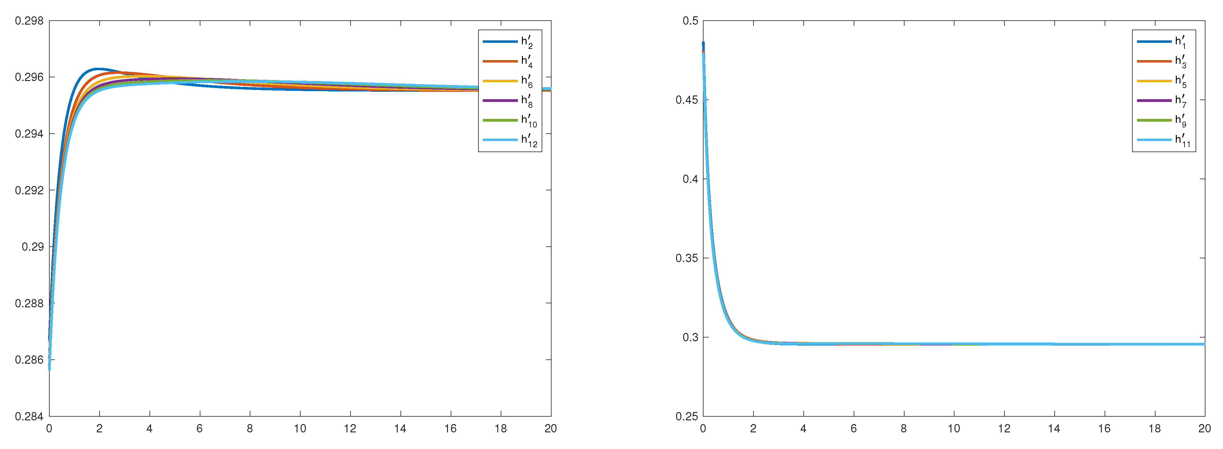
In this section, we first construct a candidate for the value function by letting m for the sequences ( g 2 m + 1 ) , ( g 2 m + 2 ) , ( g 2 m + 1 ) , ( g 2 m + 2 ) , ( h 2 m + 1 ) and ( h 2 m + 2 ) . Then, we prove the candidate to be the value function via a verification theorem.
We know from Remarks 5 and 7 that the sequences ( g 2 m + 1 ) , ( g 2 m + 2 ) , ( g 2 m + 1 ) , ( g 2 m + 2 ) , ( h 2 m + 1 ) and ( h 2 m + 2 ) are monotone and thus pointwise convergent. In the following lemma, we show that the convergence is uniform on compacts.
Lemma 9.
The sequences ( g 2 m + 1 ) , ( g 2 m ) , ( g 2 m + 1 ) , ( g 2 m ) , ( g 2 m + 1 ) , ( g 2 m ) , h 2 m , h 2 m + 1 converge uniformly on compacts to g 1 , g 2 , ( g 1 ) , ( g 2 ) , ( g 1 ) , ( g 2 ) , h 2 = g 2 1 , h 1 = g 1 1 , respectively.
Proof. 
Note first that Lemma 8 and Remark 7 yield the monotonicity of the sequences ( g 2 m + 1 ) , ( g 2 m ) , ( g 2 m + 1 ) , ( g 2 m ) , h 2 m and h 2 m + 1 . Therefore, these sequences converge pointwise implying the pointwise convergence of ( g 2 m + 1 ) and ( g 2 m ) .
In the following, we show that ( g 2 m + 1 ) , ( g 2 m + 1 ) , ( g 2 m + 1 ) and h 2 m + 1 converge uniformly on compacts.
Assume ( g 2 m + 1 ) , ( g 2 m + 1 ) , ( g 2 m + 1 ) and h 2 m + 1 converge pointwise to g 1 , w, u and χ , respectively. Note that it holds by definition of g 2 m + 1 : U m ( g 2 m + 1 ) = 0 with U m defined in (23). As g 2 m + 1 > 0 and g 2 m + 1 > 0 , see Step 2 m + 1 , it holds
λ μ 2 θ 1 2 2 μ 2 g 2 m + 1 ( x ) < λ μ θ 1 η ( g 2 m + 1 ( x ) B 1 1 ) .
Integrating both sides of the above inequality, yields
λ μ 2 θ 1 2 2 μ 2 g 2 m + 1 ( x ) g 2 m + 1 ( 0 ) = 0 x g 2 m + 1 ( y ) d y < 2 μ 2 λ μ θ 1 η λ μ 2 θ 1 2 0 x ( g 2 m + 1 ( y ) B 1 1 ) d y = 2 μ 2 λ μ θ 1 η λ μ 2 θ 1 2 g 2 m + 1 ( x ) B 1 x ,
which means that the sequence ( g 2 m + 1 ) is dominated by an integrable function. By Lebesgue’s convergence theorem 0 x g 2 m + 1 ( y ) d y converges pointwise to 0 x u ( y ) d y . Recall that 0 x u ( y ) d y is a continuous function of x and because of the uniqueness of the pointwise limit ( g 2 m + 1 ) converges pointwise to w = 0 x u ( y ) d y . That is, as ( g 2 m + 1 ) is a decreasing sequence, Dini’s theorem yields the uniform convergence of ( g 2 m + 1 ) to w on compacts.
With the same arguments we get that ( g 2 m + 1 ) converges uniformly to g 1 and it holds w = g 1 on compacts.
In a similar way, one can conclude that ( g 2 m ) and ( g 2 m ) converge uniformly on compacts to g 2 and g 2 , respectively. So that we can conclude, compare, for instance, (de Souza and Silva 2001, pp. 60, 297), that the sequence of the inverse functions ( h 2 m ) converges uniformly on compacts to h 2 , the inverse of g 2 .
As a consequence of Differential Equation U m ( g 2 m + 1 ) = 0 , also the sequence ( g 2 m + 1 ) converges uniformly to g 1 on compacts.    □
Lemma 10.
The limiting functions g 1 , g 2 , h 1 and h 2 fulfil on ( 0 , )
  • g i ( 0 ) = h i ( 0 ) = 0 ;
  • g 1 ( 1 / B ˜ 1 , 1 / Λ ) , h 1 ( Λ , B ˜ 1 ) ;
  • g 2 ( 1 / Λ , 1 / B ˜ 2 ) , h 2 ( B ˜ 2 , Λ ) ;
  • g 1 ( x ) > 0 and g 2 < 0 ;
  • h 1 ( x ) > 0 and h 2 ( x ) < 0 .
  • g 1 , g 2 , h 1 and h 2 fulfil on ( 0 , )
    λ μ 2 θ 1 2 2 μ 2 g 1 ( x ) = λ μ θ 1 η ( g 1 ( x ) B 1 1 ) + q 11 g 1 ( x ) e h 2 ( g 1 ( x ) ) + x , λ μ 2 θ 2 2 2 μ 2 g 2 ( x ) = λ μ θ 2 η ( g 2 ( x ) B 2 1 ) + q 22 g 2 ( x ) e h 1 ( g 2 ( x ) ) + x .
Proof. 
From Lemma 9, one gets immediately the above inequalities with ≥ and ≤ instead of > and < along with Differential Equation (26).
The strict inequalities follow easily using the methods presented in Step 1.    □
Lemma 11.
For i { 1 , 2 } it holds lim x g i ( x ) = 1 / Λ and lim x g i ( x ) = 0 .
Proof. 
Note that g 1 is increasing and g 2 is decreasing with g 1 1 / Λ , g 2 1 / Λ , h 1 Λ and h 2 Λ . It means
h 2 ( g 1 ( x ) ) g 1 ( x ) + 1 0 a n d h 1 ( g 2 ( x ) ) g 2 ( x ) + 1 0 ,
meaning that e h 2 ( g 1 ( x ) ) + x is increasing and e h 1 ( g 2 ( x ) ) + x is decreasing. If lim x g 1 ( x ) < 1 / Λ , then lim x e h 2 ( g 1 ( x ) ) + x = contradicting g 1 0 . If lim x g 2 ( x ) > 1 / Λ , then lim x e h 2 ( g 2 ( x ) ) + x = 0 leads to the contradiction lim x g 2 ( x ) > 0 .
lim x g i ( x ) = 0 is a direct consequence from the above.    □
Corollary 3.
It holds x e h i ( y ) d y < , i { 1 , 2 } .
Proof. 
As h 1 ( 0 ) = 0 = h 2 ( 0 ) and h 1 ( Λ , B ˜ 1 ) and h 2 ( B ˜ 2 , Λ ) we conclude h 1 ( Λ x , B ˜ 1 x ) and h 2 ( B ˜ 2 x , Λ x ) . Therefore,
x e h i ( y ) d y < x e B ˜ 2 y d y < .
   □
Definition 1.
We let for i { 1 , 2 }
V ˜ ( i , x ) : = x e h i ( y ) d y
and
b ( i , x ) : = μ θ i μ 2 h i ( x ) .
Lemma 12.
The function V ˜ and b defined in (27) and (28), respectively, fulfil
  • V ˜ ( i , x ) = e h i ( x ) , b ( i , x ) ( 0 , 1 ) .
  • V ˜ ( i , x ) solves the system of differential equations for i , j { 1 , 2 } with i j
    λ μ 2 b ( i , x ) 2 2 V ˜ ( i , x ) + λ μ ( θ i b ( i , x ) θ i + η ) V ˜ ( i , x ) ( δ q i i ) V ˜ ( i , x ) q i i V ˜ ( j , x ) = 0
    with the boundary conditions V ˜ ( i , 0 ) = 1 and lim x V ˜ ( i , x ) = 0 .
  • V ˜ ( i , x ) is the return function corresponding to the strategy b ( i , x ) .
Proof. 
  • It follows directly from (27), (28), (11), h 2 ( B ˜ 2 , Λ ) and h 1 ( Λ , B ˜ 1 ) .
  • The functions g 1 , g 2 , h 1 and h 2 solve the system of equations (26) with boundary conditions g 1 ( 0 ) = g 2 ( 0 ) = 0 , lim x g 1 ( x ) = lim x g 1 ( x ) = 1 / Λ and g 1 ( h 1 ( x ) ) = x , g 2 ( h 2 ( x ) ) = x .
    It holds V ˜ ( 1 , g i ( x ) ) = e x , i.e.,
    V ˜ ( i , g i ( x ) ) = e x g i ( x ) a n d V ˜ ( i , g i ( x ) ) = e x g i ( x ) 2 e x g i ( x ) g i ( x ) 3 .
    Substituting g i by V ˜ ( i , x ) in (26) yields the desired result.
  • Similar to Shreve et al. (1984) and Section 3, one gets that
    V ˜ ( i , x ) = E 0 e δ t d Y t b ,
    where { Y t B } describes the capital injection process corresponding to the strategy B = { b } with b defined in (28).
   □
Proposition 2.
The function V ˜ ( i , x ) defined in (27) is strictly decreasing, convex, fulfils V ( i , 0 ) = 1 , lim x V ( i , x ) = 0 and solves HJB Equation (4).
Proof. 
The proof follows easily from Lemma 12.    □
Theorem 1 (Verification Theorem).
The strategy B = { b } with
b ( i , x ) = μ θ i μ 2 h i ( x ) < 1
is the optimal strategy, and the corresponding return function V ˜ , given in (27), is the value function.
Proof. 
Let B = { b t } be an arbitrary admissible strategy and X B the surplus process under B and after the capital injections. Following the steps from lemma 1 we get
e δ ( t ) V ˜ ( J t , X t B ) = V ˜ ( J 0 , X 0 B ) + 0 t e δ s V ˜ ( J s , X s B ) d W s + M t + 0 t e δ s { λ μ 2 b s 2 2 V ˜ ( J s , X s B ) + λ μ ( θ J s b s θ J s + η ) V ˜ ( J s , X s B ) ( δ q J s , J s ) V ˜ ( J s , X s B ) q J s , J s V ˜ 1 1 [ J s = 1 ] + 1 , X s B } d s + 0 t e δ s V ˜ ( J s , X s B ) d Y s B
where M is again a martingale with expectation 0 as M is bounded
| V ˜ ( X s B , j ) V ˜ ( X s B , J s ) | max i { 1 , 2 } V 1 ( X s B , i ) ,
where V 1 is the return function corresponding to the strategy “no reinsurance”, i.e., b 1 . Because V ˜ is bounded we can conclude that also the stochastic integral is a martingale with expectation zero. Further, as V ˜ solves the HJB equation and is convex with V ( i , 0 ) = 1 , it follows that
λ μ 2 b s 2 2 V ˜ ( J s , X s B ) + λ μ ( θ J s b s θ J s + η ) V ˜ ( J s , X s B ) ( δ q J s , J s ) V ˜ ( J s , X s B ) q J s , J s V ˜ 1 1 [ J s = 1 ] + 1 , X s B 0
and V ˜ ( i , x ) 1 . Thus, building expectations on the both sides in (29) yields
E e δ t V ˜ ( J t , X t B ) V ˜ ( i , x ) E 0 t e δ s d Y s B .
By the bounded convergence theorem, we can interchange limit t and expectations and get V ˜ ( i , x ) E 0 e δ s d Y s B . For the strategy B = { b ( J s , X s ) } , we get the equality.    □

6. Numerical Illustrations

All numerical computations were performed on Matlab R2020b using the library bvpsuite2.01.
The package bvpsuite2.0 has been developed at the Institute for Analysis and Scientific Computing, Vienna University of Technology, and can be used—among other applications—for the numerical solution of boundary value problems in ordinary differential equations on semi-infinite intervals. The library uses collocation for the numerical solution of the underlying boundary value problems, which is a piecewise polynomial function which satisfies the given ODE at a finite number of nodes (collocation points). This approach shows advantageous convergence properties compared to other direct higher order methods.2
The subsequent example has an illustrative scope and aims solely at providing numerical evidence of the convergence of the recursive algorithm developed in the previous theoretical sections. In order to provide a clear numerical illustration of the results, the following choice of parameters turns out to be suitable: μ = 1 , λ = 1 , μ 2 = 4 , η = 0.3 , θ 1 = 0.33 , θ 2 = 0.8 , q 11 = 0.6 and q 22 = 0.4 .

6.1. Illustration of the Recursive Procedure

We start with illustrating the recursive procedure described in Section 4; that is, we consider the functions h 2 k and h 2 k + 1 and their convergence behaviour.
The fast convergence of each h i ( x ) Λ for x results in a very badly conditioned differential equation (in this example, Λ 0.295522 ). As a consequence, we had to truncate the solution interval and set the boundary conditions at x = 500 , i.e., h i ( 500 ) = Λ . The short horizon leads the solver to overshoot the solution at the beginning and to compensate later on, creating a characteristic initial “hump” for h 2 k + 1 , which is evened out more and more with each iteration. As a matter of fact, the larger k is, the more h 2 k + 1 is converging towards a concave shape. On the other hand, the convergence of h 2 k is faster, as for 6 iterations the functions are already very close to each other, see Figure 1.

6.2. Solving the HJB Directly

Differently than in the section above, the HJB Equation (4) is now solved directly using again bvpsuite2.0. The optimal reinsurance strategy b ( i , x ) and the ratio V ( i , x ) V ( i , x ) corresponding to the limit of the sequences ( h 2 m + 1 ) (for i = 1 ) and ( h 2 m ) (for i = 2 ) are illustrated in Figure 2.
In Figure 2, left picture, one sees that in both regimes the optimal reinsurance strategy is non-constant with respect to the surplus level. The red line representing the optimal strategy b ( 1 , x ) is decreasing and the strategy b ( 2 , x ) , in blue, is increasing. The reason for this behaviour is the relation B ˜ 1 > Λ > B ˜ 2 , where B ˜ 1 = 1.787083 and B ˜ 2 = 0.24 . The optimal strategies for the one-regime cases are
μ θ 1 μ 2 B ˜ 1 = 0.046165 < μ θ 1 μ 2 Λ = 0.350947
for the regime 1 and
μ θ 2 μ 2 B ˜ 2 = 0.83 > μ θ 1 μ 2 Λ = 0.676769
for regime 2, respectively. Thus, due to the possibility to change into a regime with a different reinsurance price, the optimal strategy changes.
In Figure 2, right picture, we see that the ratio V ( i , x ) V ( i , x ) converges for both regimes to the level 0.295522 = Λ , the value towards which the sequences h 2 k and h 2 k + 1 converge as can be seen in Section 6.1.
Using bvpsuite optimisation, each step of the iteration takes between 30 and 40 s to compute on a single 3GHz core.
These findings confirm the validity of the iterative algorithm developed in Section 4 and illustrated numerically in Section 6.1.

7. Conclusions

In this paper, we study the problem faced by an insurance company that aims at finding the optimal proportional reinsurance strategy minimising the expected discounted capital injections. We assume that the cost of entering the proportional reinsurance contract depends on the current busyness cycle of a two-state economy, and we model this by letting the safety loading of the reinsurance be modulated by a continuous-time Markov chain. This leads to an optimal reinsurance problem under regime switching. In order to simplify our explanations, we assume a certain relation between the crucial parameters of the two regimes. Considering all possible combinations would be space-consuming with just a marginal additional value.
Differently to Eisenberg and Schmidli (2009)—where no regime switching has been considered—we find that the optimal reinsurance cannot be independent of the current value of the surplus process, but should instead be given as a feedback strategy b , also depending on the current regime. However, due to the complex nature of the resulting HJB equation, determining an explicit expression for b 
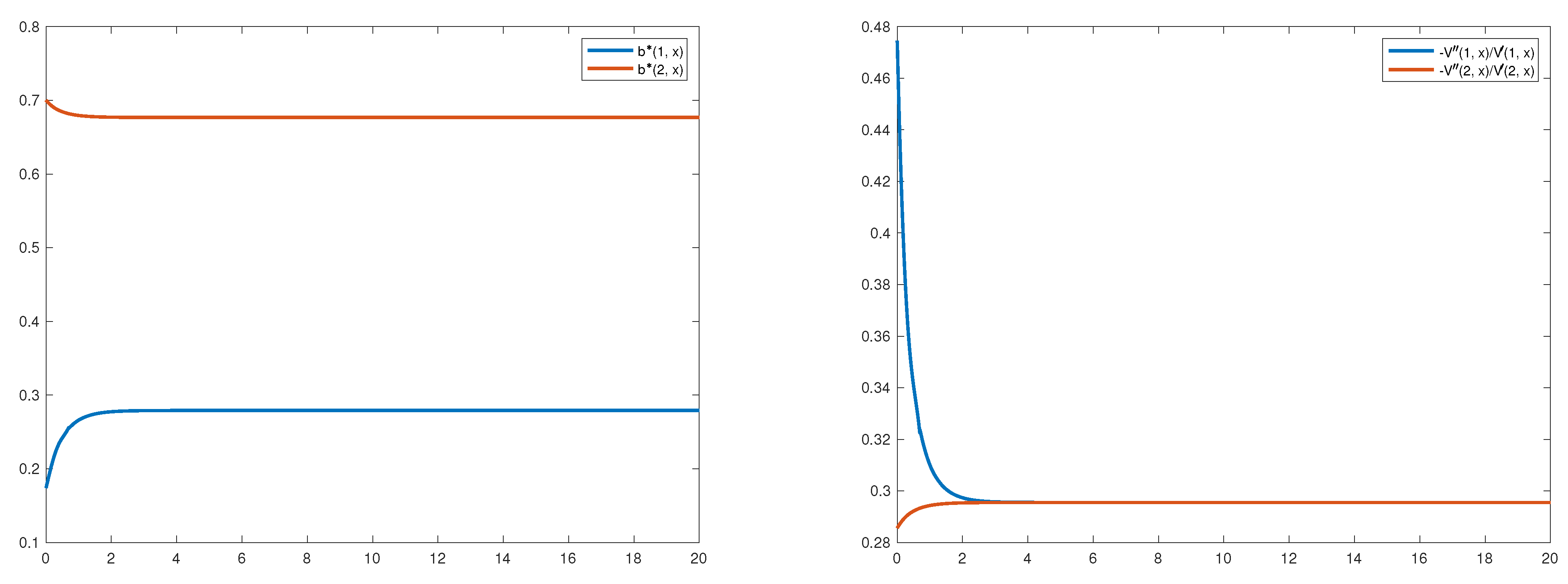
turns out to be a challenging task. For this reason, we develop a recursive algorithm that hinges on the construction of two sequences of functions converging uniformly to a classical solution to the HJB equation and simultaneously providing the optimal strategies for both regimes. The obtained optimal strategies are monotone with respect to the surplus level and converge for both regimes to the same explicitly calculated constant as the surplus goes to infinity. The algorithm is illustrated by a numerical example, where one can also see that the convergence to the solution of the HJB equation is quite fast.
The recursive scheme represents the main contribution of this paper and might also be applied (with necessary adjustments) to other optimisation problems containing regime-switching. For this reason, we retrace here the main steps and ideas of the algorithm.
The differential equation for the value function is first translated into a differential equation for an auxiliary function, transforming the derivative of the value function into an exponential function, using the method of Højgaard and Taksar (1998). In order to get a solution to the system of equations, say Equations (a) and (b), we solve the differential Equation (a) assuming that the solution to Equation (b) is given by an exponential function e Λ , which is the starting function of our algorithm. Then, we solve Equation (b) by inserting the solution to Equation (a) from the previous step. Proceeding in this manner, we obtain two sequences of uniformly converging functions whose limiting functions solve the original HJB equation system.
Note that we are facing a boundary value problem, i.e., the boundary conditions on the value function and its derivative, lim x V ( i , x ) = 0 and V ( i , 0 ) = 1 are given at different boundaries, with one boundary being infinity. Therefore, the usual Picard–Lindelöf approach does not work. Instead, we use Volterra form representations and comparison theorems to show the existence and uniqueness of a solution with the desired properties.
One of the crucial points in the above considerations is the starting function of the algorithm. It turns out that there is a uniquely given constant, Λ , allowing to obtain the desired properties of the limiting functions.
In particular, we show that the derivatives of the auxiliary functions lie in suitable intervals ( B ˜ 2 , Λ ) or ( Λ , B ˜ 1 ) , depending on the differential equation we are looking at.
Thus, we are able to show that the value function is twice continuously differentiable and the optimal strategy has a monotone character and converges for x to an explicitly calculated value.
It would be interesting to implement the considerations from Chiappori et al. (2006) to extend the presented model by hidden information, for instance, by introducing a hidden Markov chain governing the reinsurance price over the parameter θ . This topic will be one of the directions of our future research.

Author Contributions

J.E.: Conceptualisation, methodology, formal analysis, writing—original draft preparation abs writing—review and editing; supervision abs project administration. L.F.: visualisation abs numerical results. M.D.S.: Conceptualisation, minor methodology, minor formal analysis abs writing—original draft preparation. All authors have read and agreed to the published version of the manuscript.

Funding

The research of Julia Eisenberg was funded by the Austrian Science Fund (FWF), Project number V 603-N35. Maren Diane Schmeck acknowledges financial support by the German Research Foundation (DFG) through the Collaborative Research Centre 1283 “Taming uncertainty and profiting from randomness and low regularity in analysis, stochastics and their applications”.

Institutional Review Board Statement

Not applicable.

Informed Consent Statement

Not applicable.

Data Availability Statement

Not applicable.

Acknowledgments

The authors would like to thank the anonymous referees for their comments and suggestions that helped to considerably improve the paper.

Conflicts of Interest

The authors declare no conflict of interest.

Appendix A

Appendix A.1. Proofs of Step 1

Proof of Lemma 4.
Let n N and consider the differential Equation (17) on the interval [ 0 , n ] with the boundary conditions g ( 0 ) = 0 and g ( 0 ) = ϑ for some ϑ > 0 .
  • It is straightforward to show that Equation (17) can be written in form of a Volterra integral equation
    λ μ 2 θ 1 2 2 μ 2 g ( x ) = λ μ 2 θ 1 2 2 μ 2 ϑ + q 11 Λ x λ μ ( θ 1 η ) 2 x 2 + 0 x λ μ ( θ 1 η ) B 1 g ( z ) + q 11 Λ e Λ g ( z ) + z ( x z 1 ) d z
    Note that the function
    k ( x , z , y ) : = λ μ ( θ 1 η ) B 1 y + q 11 Λ e Λ y + z ( x z 1 )
    is Lipschitz continuous in y for x [ 0 , n ] . Then, the Theorem on Continuous Dependence, see Walter (Walter 1998, p. 148), yields the existence of a unique solution ξ n ( x ; ϑ ) to (17) on [ 0 , n ] with ξ n ( 0 ; ϑ ) = 0 and ξ n ( 0 ; ϑ ) = ϑ for every ϑ [ 1 / B ˜ 1 , 1 / Λ ] , where ξ ( x ; ϑ ) is continuous as a function of ( x ; ϑ ) .
    From Lemma 3, we know that ξ n ( n ; 1 / B ˜ 1 ) < 1 / Λ and ξ n ( n ; 1 / Λ ) > 1 / Λ . By the intermediate value theorem, there is a ϑ n ( 1 / B ˜ 1 , 1 / Λ ) leading to a solution ξ n ( x ; ϑ n ) with ξ n ( 0 ; ϑ n ) = 0 and ξ n ( n ; ϑ n ) = 1 / Λ .
  • Further, letting
    f ( x , y 1 , y 2 ) = f 1 ( x , y 1 , y 2 ) , f 2 ( x , y 1 , y 2 ) : = y 2 , 2 μ 2 λ μ ( θ 1 η ) λ μ 2 θ 1 2 ( B 1 y 2 1 ) + 2 μ 2 q 11 λ μ 2 θ 1 2 y 2 e Λ y 1 + x
    on D : = R + × 1 / B ˜ 1 , 1 / Λ × R we can rewrite Differential Equation (17) as a system of first-order equations:
    ( y 1 , y 2 ) = f ( x , y 1 , y 2 ) .
The Jacobi matrix J = ( c i j ) = ( d f i / d y j ) is then given by
J = 0 1 2 μ 2 q 11 λ μ 2 θ 1 2 y 2 Λ e Λ y 1 + x 2 μ 2 λ μ ( θ 1 η ) λ μ 2 θ 1 2 B 1 + 2 μ 2 q 11 λ μ 2 θ 1 2 e Λ y 1 + x .
On D, the Jacobi matrix J is essentially positive3 and irreducible4. We can conclude that by Hirsch’s Theorem, see Walter (Walter 1998, p. 112), for any ϑ < ϑ ˜ it holds ξ n ( x ; ϑ ) < ξ n ( x ; ϑ ˜ ) and ξ n ( x ; ϑ ) < ξ n ( x ; ϑ ˜ ) for all x ( 0 , n ] . Therefore, ξ n ( x ; ϑ n ) is the unique solution to (17) with the boundary conditions ξ n ( 0 ; ϑ n ) = 0 and ξ n ( n ; ϑ n ) = 1 / Λ . For simplicity, we will write for this unique solution just ξ n ( x ) . □
Proof of Lemma 5.
We know from Lemma 3 that ξ n ( 0 ) ( 1 / B ˜ 1 , 1 / Λ ) . Then, it holds that ξ n ( 0 ) > 0 and e Λ ξ n ( x ) + x is increasing as long as ξ n < 1 / Λ . Further, deriving (17) we get
λ μ 2 θ 1 2 2 μ 2 ξ n ( x ) = ξ n ( x ) B 1 λ μ θ 1 η + q 11 ξ n ( x ) e Λ ξ n ( x ) + x + q 11 ξ n ( x ) Λ ξ n ( x ) + 1 e Λ ξ n ( x ) + x .
Let x ^ : = inf { x > 0 : ξ n ( x ) = 0 } . Then, ξ n ( x ) > 0 and consequently ξ n ( x ) > 1 / B ˜ 1 on [ 0 , x ^ ) . If x ^ [ 0 , n ) , then
ξ n ( x ^ ) = q 11 ξ n ( x ^ ) Λ ξ n ( x ^ ) + 1 e Λ ξ n ( x ^ ) + x ^ < 0 : ξ n ( x ^ ) < 1 / Λ , > 0 : ξ n ( x ^ ) > 1 / Λ .
  • Thus, if ξ n ( x ^ ) < 1 / Λ , then ξ n ( x ^ ) < 0 and the second derivative ξ n becomes negative, implying that ξ n stays smaller than 1 / Λ on [ x ^ , n ] and contradicts ξ n ( n ) = 1 / Λ .
  • If ξ n ( x ^ ) > 1 / Λ , then ξ n ( x ^ ) > 0 contradicting ξ n ( x ^ ) = 0 .
  • If ξ n ( x ^ ) = 1 / Λ , then ξ n ( x ^ ) = 0 implying ξ n ( k ) ( x ^ ) = 0 for all k 4 . This means that ξ n ( x ) is a linear function on [ 0 , n ] , i.e., ξ n ( x ) is a constant and ξ n ( x ) 0 on [ 0 , n ] . Inserting this conjecture into Differential Equation (17) yields the contradiction.
If x ^ > n the claim follows with the arguments from Lemma 3. □
Proof of Proposition 1.
  • First, we show that the sequences ( ξ n ) and ( ξ n ) are decreasing.
    As it holds ξ n ( n ) = 1 / Λ for all n 1 , with Lemma 5 one gets ξ n ( x ) > 1 / Λ for x > n . This means, in particular, that ξ n + 1 ( n + 1 ) = 1 / Λ < ξ n ( n ) .
    We know that ξ n ( 0 ) = 0 = ξ n + 1 ( 0 ) . Assume now ξ n + 1 ( 0 ) ξ n ( 0 ) . The function
    F ( x , y 1 , y 2 ) = 2 μ 2 λ μ 2 θ 1 2 λ μ ( θ 1 η ) { y 2 B 1 1 } + q 11 y 2 e Λ y 1 + x
    is increasing in y 1 . Letting P f : = f F ( x , f , f ) Differential Equation (17) can be written as P ξ n = 0 = P ξ n + 1 . Comparison Theorem, see Walter (Walter 1998, p. 139), yields then ξ n ( x ) ξ n + 1 ( x ) on [ 0 , n + 1 ] leading to a contradiction.
    Thus, ξ n ( 0 ) > ξ n + 1 ( 0 ) for all n N and as a direct consequence of the same Comparison Theorem: ξ n ( x ) ξ n + 1 ( x ) and ξ n ( x ) ξ n + 1 ( x ) on compacts for all n N .
    Therefore, we can conclude that the sequences ( ξ n ) and ( ξ n ) are decreasing fulfilling ξ n ( 0 ) = 0 and ξ n ( n ) = 1 / Λ . Therefore, ( ξ n ) and ( ξ n ) converge pointwise to some functions g 1 and w, respectively, and due to Differential Equation (17), the sequence ( ξ n ) converges pointwise to some function u.
  • In the next step, we show that the sequences ( ξ n ) , ξ n and ( ξ n ) converge uniformly on compacts.
    As ξ n > 0 and ξ n > 0 , see Lemma 5, for all n 1 and all x 0 , it holds that
    λ μ 2 θ 1 2 2 μ 2 ξ n ( x ) = ( ξ n ( x ) B 1 1 ) λ μ θ 1 η + q 11 ξ n ( x ) e Λ ξ n ( x ) + x < ( ξ n ( x ) B 1 1 ) λ μ θ 1 η .
    Integrating both sides of the above inequality and using that ξ n ξ n + 1 , yields
    ξ n ( x ) ξ n ( 0 ) = 0 x ξ n ( y ) d y < 2 μ 2 λ μ θ 1 η λ μ 2 θ 1 2 0 x ( ξ 1 ( y ) B 1 1 ) d y = 2 μ 2 λ μ θ 1 η λ μ 2 θ 1 2 ξ 1 ( x ) B 1 x ,
    which means that the sequence ( ξ n ) is dominated by a locally integrable function. By Lebesgue’s convergence theorem 0 x ξ n ( y ) d y converges pointwise to 0 x u ( y ) d y . Recall that 0 x u ( y ) d y is a continuous function of x, and because of the uniqueness of the pointwise limit, ( ξ n ) converges pointwise to w = 0 x u ( y ) d y . That is, as ( ξ n ) is a decreasing sequence Dini’s theorem yields the uniform convergence of ( ξ n ) to w on compacts.
    With the same argument, we get that ( ξ n ) converges uniformly to g 1 and it holds w = g 1 on compacts. As a consequence of Differential Equation (17), ( ξ n ) converges uniformly to g 1 on compacts.
  • Now, we are ready to show that g 1 fulfils lim x g 1 ( x ) = 1 / Λ .
    Note that g 1 solves Equation (17). The function g 1 fulfils due to the properties of ( ξ n ) and ( ξ n ) : g 1 ( 0 ) = 0 , g 1 ( x ) 1 / B ˜ 1 and g 1 ( x ) 0 for all x 0 . It means that lim x g 1 ( x ) ( 1 / B ˜ 1 , ] . If lim x g 1 ( x ) > 1 Λ then there is an m N such that g 1 ( x ) > 1 Λ for x m . However, for ξ n with n > m it holds ξ n ( m ) < 1 Λ , meaning g 1 ( m ) 1 Λ . Then, we can conclude that lim x g 1 ( x ) 1 Λ .
    If lim x g 1 ( x ) < 1 Λ then lim x e Λ g 1 ( x ) + x = . However, the differential equation for g 1 yields
    λ μ 2 θ 1 2 2 μ 2 g 1 ( x ) = λ μ 2 θ 1 2 2 μ 2 g 1 ( x ) λ μ θ 1 η + ( δ q 1 ) g 1 ( x ) + q 11 g 1 ( x ) e Λ g 1 ( x ) + x a s x ,
    contradicting g 1 > 0 .
    Therefore, we conclude lim x g 1 ( x ) = 1 Λ . With the arguments from Lemma (5), we can conclude g 1 > 0 on ( 0 , ) and lim x g 1 ( x ) = 0 .

Appendix A.2. Proofs of Step 2

Proof of Lemma 6.
  • Assume for the moment that g 2 ( 0 ) = 1 / Λ . Then,
    λ μ 2 θ 2 2 2 μ 2 g 2 ( 0 ) = λ μ θ 2 η ( g 2 ( 0 ) B ˜ 2 1 ) < 0
    and h 1 ( 0 ) g 2 ( 0 ) + 1 < 0 . Therefore, g 2 ( x ) < 1 / Λ on ( 0 , ε ) and
    λ μ 2 θ 2 2 2 μ 2 g 2 ( x ) = λ μ θ 2 η ( g 2 ( x ) B 2 1 ) + q 22 g 2 ( x ) e h 1 ( g 2 ( x ) ) + x = λ μ θ 2 η ( g 2 ( x ) B 2 1 ) + q 22 g 2 ( x ) e h 1 ( g 2 ( x ) ) + Λ ξ n ( x ) Λ g 2 ( x ) + x ,
    As h 1 > Λ , it holds that h 1 ( x ) + Λ < 0 , and (22) gives lim x ( h 1 ( x ) + Λ x ) = α and consequently h 1 ( x ) + Λ x > α . Furthermore, as long as g 2 1 / Λ the function e Λ g 2 + x is increasing giving e Λ g 2 + x 1 . Thus, on ( 0 , ε ) ,
    λ μ 2 θ 2 2 2 μ 2 g 2 ( x ) < λ μ θ 2 η ( g 2 ( x ) B 2 1 ) + q 22 g 2 ( x ) e α e Λ g 2 ( x ) + x λ μ θ 2 η ( g 2 ( x ) B 2 1 ) + q 22 g 2 ( x ) e α .
    Because α > 0 , see (15), it holds that B 2 + q 22 e α > 0 , meaning that the rhs in the above inequality is strictly increasing in g 2 . Therefore, we can conclude using (15):
    λ μ 2 θ 2 2 2 μ 2 g 2 ( x ) < λ μ θ 2 η B 2 Λ 1 + q 22 Λ e α = 0 ,
    i.e., g 2 remains negative and the boundary value 1 / Λ would be never attained if g 2 ( 0 ) = 1 / Λ .
  • Assume now g 2 ( 0 ) = 1 / B ˜ 2 . Then, ξ n ( 0 ) = 0 and because h 1 ( 0 ) > Λ (Corollary 1) it holds
    λ μ 2 θ 2 2 2 μ 2 g 2 ( 0 ) = q 22 g 2 ( 0 ) g 2 ( 0 ) h 1 ( 0 ) + 1 > 0 .
    We conclude that g 2 > 0 and ξ n > 1 / B ˜ 2 on ( 0 , ε ) . However, if x ^ : = inf { x > ε : g 2 ( x ) = 0 } ( ε , ) it holds g 2 ( x ^ ) > 0 contradicting g 2 ( x ^ ) = 0 . Hence, g 2 will stay above 1 / B ˜ 2 .
  • By Hirsch’s Theorem, see Walter (Walter 1998, p. 112), for g 2 ( 0 ) ( 1 / Λ , 1 / B ˜ 2 ) it holds g 2 ( n ) 1 / Λ .

Appendix A.3. Proofs of Step 2m+1

Proof of Lemma 8.
Note first that h 2 and h 0 fulfil the above assumptions.
To prove the claim for a general m, we consider the difference of the differential equations U m ( g 2 m + 1 ) U m 1 ( g 2 m 1 ) = 0 :
λ μ 2 θ 1 2 2 μ 2 g 2 m + 1 ( x ) g 2 m 1 ( x ) = B 1 λ μ θ 1 η { g 2 m + 1 ( x ) g 2 m 1 ( x ) } + q 11 g 2 m + 1 ( x ) e h 2 m ( g 2 m + 1 ( x ) ) + x q 11 g 2 m 1 ( x ) e h 2 m 2 ( g 2 m 1 ( x ) ) + x .
  • If g 2 m + 1 ( 0 ) = g 2 m 1 ( 0 ) , then all k-th derivatives k N fulfil g 2 m + 1 ( k ) ( 0 ) = g 2 m 1 ( k ) ( 0 ) , implying g 2 m + 1 ( x ) = g 2 m 1 ( x ) for all x. As U m 1 ( g 2 m + 1 ) 0 because h 2 m < h 2 m 2 for x > 0 , we get a contradiction.
  • In this part, we show that g 2 m + 1 ( 0 ) < g 2 m 1 ( 0 ) is impossible.
    For that purpose, we use again the auxiliary functions introduced in Lemma 4, representing the solutions to differential equations with boundary conditions at 0 and at n N . We denote by ξ m 1 , n the solutions to U m 1 ( ξ m 1 , n ) = 0 with the boundary conditions ξ m 1 , n ( 0 ) = 0 and ξ m 1 , n ( n ) = 1 / Λ and by ξ m , n the solutions to U m ( ξ m , n ) = 0 with boundary conditions ξ m , n ( 0 ) = 0 and ξ m , n = 1 / Λ , for n N .
    Let n be arbitrary, but fixed and assume ξ m , n ( 0 ) < ξ m 1 , n ( 0 ) . Let further x ^ : = inf { x > 0 : ϕ n ( x ) = ψ n ( x ) } . Then, it holds ξ m , n ( x ) < ξ m 1 , n ( x ) and ξ m , n ( x ) < ξ m 1 , n ( x ) on ( 0 , x ^ ) . This means in particular, using the properties of h 2 m and h 2 m 2 , that h 2 m ( ξ m , n ( x ^ ) ) < h 2 m 2 ( ξ m 1 , n ( x ^ ) ) and consequently
    q 11 ξ m , n ( x ^ ) e h 2 m ( ξ m , n ( x ^ ) ) + x ^ q 11 ξ m 1 , n ( x ^ ) e h 2 m 2 ( ξ m 1 , n ( x ^ ) ) + x ^ < 0 .
    Equality (A2) then yields ξ m , n ( x ^ ) ξ m 1 , n ( x ^ ) < 0 , contradicting ξ m , n ( x ^ ) ξ m 1 , n ( x ^ ) = 0 .
    That is, we can conclude ξ m , n ( x ) ξ m 1 , n ( x ) < 0 for all x 0 . However, this contradicts ξ m 1 , n ( n ) = 1 / B 2 = ξ m , n ( n ) . Furthermore, we conclude ξ m 1 , n ( 0 ) > ξ m , n ( 0 ) leading via the uniform convergence, see Lemma 4, to g 2 m + 1 ( 0 ) g 2 m 1 ( 0 ) . As we excluded g 2 m + 1 ( 0 ) = g 2 m 1 ( 0 ) , it must hold g 2 m + 1 ( 0 ) > g 2 m 1 ( 0 ) .
  • We know already that it must hold g 2 m + 1 ( 0 ) > g 2 m 1 ( 0 ) .
    Let z ^ : = inf { x > 0 : g 2 m + 1 ( x ) < g 2 m 1 ( x ) } and assume that z ^ ( 0 , ) . At z ^ it holds then g 2 m + 1 ( z ^ ) g 2 m 1 ( z ^ ) = 0 and g 2 m + 1 ( z ^ ) g 2 m 1 ( z ^ ) 0 which, due to (A2), means
    0 λ μ 2 θ 1 2 2 μ 2 g 2 m + 1 ( z ^ ) g 2 m 1 ( z ^ ) = q 11 g 2 m + 1 ( z ^ ) e z ^ { e h 2 m ( g 2 m + 1 ( z ^ ) ) e h 2 m 2 ( g 2 m 1 ( z ^ ) ) } .
    Thus, h 2 m ( g 2 m + 1 ( z ^ ) ) h 2 m 2 ( g 2 m 1 ( z ^ ) ) .
    On the other hand, from Step 2 m we know that g 2 m ( x ) > g 2 m 2 on R + which is equivalent to
    h 2 m 2 ( g 2 m 2 ) > h 2 m ( g 2 m )
    on R + . As h 2 m , h 2 m 2 , g 2 m , g 2 m 2 > 0 , we can conclude that h 2 m 2 ( g 2 m 2 ) and h 2 m ( g 2 m ) are strictly increasing. For all x with h 2 m ( g 2 m + 1 ( x ) ) h 2 m 2 ( g 2 m 1 ( x ) ) , it holds that
    h 2 m 2 ( g 2 m 1 ( x ) ) = h 2 m 2 g 2 m 2 h 2 m 2 ( g 2 m 1 ( x ) ) > h 2 m g 2 m h 2 m ( g 2 m + 1 ( x ) ) = h 2 m ( g 2 m + 1 ( x ) ) .
    Thus, if additionally g 2 m 2 g 2 m , then
    d d x h 2 m 2 ( g 2 m 1 ( x ) ) > d d x h 2 m ( g 2 m + 1 ( x ) ) .
    This means in particular that g 2 m + 1 ( z ^ ) g 2 m 1 ( z ^ ) < 0 and consequently g 2 m + 1 ( x ) g 2 m 1 ( x ) < 0 for x > z ^ . As g 2 m + 1 ( z ^ ) g 2 m 1 ( z ^ ) = 0 , we obtained a contradiction to lim x g 2 m + 1 ( x ) g 2 m 1 ( x ) = 0 .

Notes

1.
2.
3.
c i j 0 for all i j .
4.
J cannot be transformed into a block upper triangle matrix via a permutation, i.e., there is no permutation matrix P leading to PJP 1 = a b 0 c .

References

  1. Asmussen, Søren. 1989. Risk theory in a Markovian environment. Scandinavian Actuarial Journal 1989: 69–100. [Google Scholar] [CrossRef]
  2. Asmussen, Søren, and Hansjorg Albrecher. 2010. Ruin Probabilities. London: World Scientific Publishing. [Google Scholar]
  3. Auzinger, Winfried, Merlin Fallahpour, Othmar Koch, and Ewa Weinmüller. 2019. Implementation of a Pathfollowing Strategy with an Automatic Step-Length Control: New MATLAB Package Bvpsuite2.0. ASC Report 31/2019. Wien: Institute for Analysis and Scientific Computing, Vienna University of Technology. [Google Scholar]
  4. Azcue, Pablo, and Nora Muler. 2005. Optimal reinsurance and dividend distribution policies in the Cramér–Lundberg model. Mathematical Finance 15: 261–308. [Google Scholar] [CrossRef]
  5. Bargès, Mathieu, Stéphane Loisel, and Xavier Venel. 2013. On finite-time ruin probabilities with reinsurance cycles influenced by large claims. Scandinavian Actuarial Journal 2013: 163–85. [Google Scholar] [CrossRef] [Green Version]
  6. Bäuerle, Nicole, and Mirko Kötter. 2007. Markov-modulated diffusion risk models. Scandinavian Actuarial Journal 2007: 34–52. [Google Scholar] [CrossRef] [Green Version]
  7. Ben Salah, Zied, and José Garrido. 2018. On fair reinsurance premiums; capital injections in a perturbed risk model. Insurance: Mathematics and Economics 82: 11–20. [Google Scholar] [CrossRef] [Green Version]
  8. Brachetta, Matteo, and Claudia Ceci. 2020. A BSDE-based approach for the optimal reinsurance problem under partial information. Insurance: Mathematics and Economics 95: 1–16. [Google Scholar] [CrossRef]
  9. Chiappori, Pierre-André, Bruno Jullien, Bernard Salanié, and Francois Salanie. 2006. Asymmetric information in insurance: General testable implications. RAND Journal of Economics 37: 783–98. [Google Scholar] [CrossRef]
  10. de Souza, Paulo Ney, and Jorge-Nuno Silva. 2001. Berkeley Problems in Mathematics. New York: Springer. [Google Scholar]
  11. Eisenberg, Julia, and Hanspeter Schmidli. 2009. Optimal control of capital injections by reinsurance in a diffusion approximation. Blätter DGVFM 30: 1–13. [Google Scholar] [CrossRef]
  12. Eisenberg, Julia, and Paul Krühner. 2018. The impact of negative interest rates on optimal capital injections. Insurance: Mathematics and Economics 82: 1–10. [Google Scholar] [CrossRef] [Green Version]
  13. Gajek, Lesław, and Marcin Rudź. 2020. General methods for bounding multidimensional ruin probabilities in regime-switching models. Stochastics, 1–16. [Google Scholar] [CrossRef]
  14. Gerber, Hans U., and Elias S. W. Shiu. 1998. On the time value of ruin. North American Actuarial Journal 2: 48–78. [Google Scholar] [CrossRef]
  15. Højgaard, Bjarne, and Michael Taksar. 1998. Optimal proportional reinsurance policies for diffusion models. Scandinavian Actuarial Journal 1998: 166–80. [Google Scholar] [CrossRef]
  16. Jacod, Jean, and Albert Shiryaev. 2003. Limit Theorems for Stochastic Processes, 2nd ed. Berlin: Springer. [Google Scholar]
  17. Jiang, Zhengjun, and Martijn Pistorius. 2012. Optimal dividend distribution under Markov regime switching. Finance and Stochastics 16: 449–76. [Google Scholar] [CrossRef] [Green Version]
  18. Pafumi, Gérard. 1998. “On the time value of ruin”, Hans U. Gerber and Elias S.W. Shiu, January 1998. North American Actuarial Journal 2: 75–76. [Google Scholar] [CrossRef]
  19. Rolski, Tomasz, Hanspeter Schmidli, Volker Schmidt, and Jozef L. Teugels. 1999. Stochastic Processes for Insurance & Finance. Hoboken: John Wiley & Sons Ltd. [Google Scholar]
  20. Schmidli, Hanspeter. 2008. Stochastic Control in Insurance. London: Springer. [Google Scholar]
  21. Schmidli, Hanspeter. 2017. Risk Theory. London: Springer. [Google Scholar]
  22. Shreve, Steven E., John P. Lehoczky, and Donald P. Gaver. 1984. Optimal consumption for general diffusions with absorbing and reflecting barriers. Siam Journal on Control and Optimization 22: 55–75. [Google Scholar] [CrossRef]
  23. Walter, Wolfgang. 1998. Ordinary Differential Equations. New York: Springer. [Google Scholar]
Figure 1. The functions h 2 k (left) and h 2 k 1 (right) for k = 1 , 2 , 3 , 4 , 5 , 6 .
Risks 09 00073 g001
Figure 2. The optimal reinsurance strategies (left) and the ratios V / V (right).
Risks 09 00073 g002
Publisher’s Note: MDPI stays neutral with regard to jurisdictional claims in published maps and institutional affiliations.

