Cumulative Prospect Theory Version with Fuzzy Values of Outcome Estimates

Abstract

Choosing solutions under risk and uncertainty requires the consideration of several factors. One of the main factors in choosing a solution is modeling the decision maker’s attitude to risk. The expected utility theory was the first approach that allowed to correctly model various nuances of the attitude to risk. Further research in this area has led to the emergence of even more effective approaches to solving this problem. Currently, the most developed theory of choice with respect to decisions under risk conditions is the cumulative prospect theory. This paper presents the development history of various extensions of the original expected utility theory, and the analysis of the main properties of the cumulative prospect theory. The main result of this work is a fuzzy version of the prospect theory, which allows handling fuzzy values of the decisions (prospects). The paper presents the theoretical foundations of the proposed version, an illustrative practical example, and conclusions based on the results obtained.

1. Introduction

The decision making theory is currently a powerful tool for the formal selection of optimal decisions under various initial conditions. Decision-making tasks can be divided into three large classes:

• Decision-making problems under certainty. The outcomes of alternative decisions coincide with the decisions themselves.
• Decision-making problems under risk conditions. The outcomes of alternative decisions depend on the decisions themselves and uncertain factors (random events). The probabilities of occurrence of relevant random events are given.
• Decision-making problems under conditions of uncertainty. The outcomes of alternative decisions depend on the decisions themselves and uncertain factors (random events). The probabilities of random events occurrence are not specified.

In decision-making problems under certainty, the Pareto concept of optimal solutions (Pareto set) is the main concept. In this set, decisions are not comparable in terms of the criteria values, and the choice of optimal decision is made based on the decision maker’s subjective preferences.

Many approaches to modeling decision maker (DM) preference systems have been proposed: additive and multiplicative weighted aggregation of criteria assessments, compromise programming, the TOPSIS method, and the analytical hierarchy process (AHP) (Uzhga-Rebrov 2016; Triantaphullou 2020; Kumar et al. 2017).

In decision-making problems under risk, the criterion for maximizing the expected value, the Hermejier criterion, the expected value maximization criterion, and the Hodja-Leman criterion are used (Uzhga-Rebrov 2016; Szpiro 2020).

In decision-making problems under uncertainty, the maximin (minimax) criterion and the Hurvitz criterion are used (Uzhga-Rebrov 2016).

The choice of decisions under risk assumes a linear dependence of the outcome’s utility on its criterion assessment. However, it has long been known that the utility of money, for example, increases nonlinearly with an increase in its amount. For the first time, D. Bernoulli tried to formalize this dependence. In 1738, he suggested that money’s importance (utility) does not increase strictly in proportion to its amount. Currently, effective methods have been developed for assessing the subjective DM utility on a set of criteria estimates with respect to the decisions.

The foundations of the expected utility theory (EUT) were laid by von Neumann and Morgenstern in 1947. Von Neumann and Morgenstern’s expected utility theory to be an axiomatic prescriptive theory. It is based on the assertion that all DMs are rational, risk-averse individuals. The utility function’s construction for the DM is based on its estimates of the deterministic equivalents. The EUT is very widespread. However, practice has shown that the DM does not always behave in accordance with the requirements of this theory. The accumulation of data about theory violations led to a revision of some of its assertions. The main of which is taking into account their DM probability of outcomes, which was excluded in the EUT.

Another impulse for the development of an alternative theory was the empirical, where the utility of outcomes depends on the ranks of the outcomes.

The accumulated experiences found its expression in the prospect theory. An initial version of this theory was presented by Kahneman and Tversky in 1979, and an in-depth version was presented in (Tversky and Kahneman 1992).

For almost all criteria in choosing decisions under the conditions of certainty and risk, their fuzzy versions have been proposed (Kaya et al. 2019; Chen et al. 2016; Aggarwal et al. 2019; Radionovs and Uzhga-Rebrovs 2016).

This work aims to present the evolution of the EUT to a cumulative prospect theory and to present and substantiate a version of this theory with fuzzy estimates of the outcomes of alternative decisions (prospects). Why is one of the goals the development of the prospects theory version to handle fuzzy outcome estimates? The reason is that, in practical decision-making tasks, there are often situations when, for various reasons, it is impossible to set unambiguous outcome estimates. It becomes necessary to correctly model the existing uncertainties. The application of fuzzy outcome estimates appears to be an appropriate approach to model these uncertainties. The paper by Uzhga-Rebrov and Kuleshova (2016) proposes a version of the prospect theory using fuzzy decision weights.

The present paper is a further step in the fuzzification of a prospect theory. In the proposed fuzzy version of the prospect theory, the uncertainty of the initial estimates is translated into uncertain estimates of the value function. The aggregation of fuzzy estimates is carried out according to the rules of the original prospect theory, taking into account the fuzzy nature of these estimates. The choice of the optimal perspective is made by comparing the resulting fuzzy estimates of the expected values.

This article is structured as follows. Section 2 presents the conceptual foundations of the probability weighting principle; Section 3 presents the basics of rank-dependent utility; Section 4 presents in detail the basics of the cumulative prospect theory; Section 5 presents a proposed version of this theory with fuzzy estimates of the prospects outcomes; Section 6 presents an illustrative example of the proposed fuzzy version; Section 7 is devoted to conclusions from the obtained results.

2. Probability Weighting

Following world practice, starting from this section, we will use different terminology. Instead of the concept of an alternative decision, we will use the wider concept of prospect. In the general case, a prospect can be understood as a set of outcomes of an alternative decision together with their estimates and probabilities of occurrence. In this sense, any alternative decision can be considered a prospect since every decision under risk is associated with many outcomes that depend on random events (states of nature).

From a decision-making perspective, the EUT is seen as a normative theory that indicates how individuals should act in risky choice situations. In Schoemaker’s paper (1982), it is stated that the EUT can be considered as a predictive or positivist theory. This is due to the fact that the theory exhibits high predictive accuracy compared to other competing approaches. However, the descriptive properties of this theory raise many questions. So, in theory, it is postulated that DM’s preferences and their attitude to risk do not depend on the probabilities of outcomes of alternative decisions. However, in works (Edwards 1954, 1962), using appropriate examples, it is shown that this is not true. Individuals under conditions of risky choices implicitly consider the probabilities of outcomes. Other convincing examples can be found in (Wakker 2010; Fehr-Duda and Epper 2012).

The main purpose of probability weighting is to replace the actual values of the outcome probabilities with values that reflect the subjective perception of these values when choosing alternatives under risk conditions.

Based on the processing of numerous empirical studies’ results, the following parametric forms of the probability weighting functions have been proposed.

1. Weighting function Karmakar (Karmakar 1979):

$$w(p)=\frac{p^{\gamma }}{p^{\gamma }+{\left(1+p\right)}^{\gamma }},0<\gamma <1.$$

(1)

2. Probability weighting function Prelec-I (Prelec 1998):

$$w(p)=\frac{1}{e^{{\left(-lnp\right)}^{\alpha }}},0<\alpha <1.$$

(2)

3. Probability weighting function Prelec-II (Prelec 1998):

$$w(p)=\frac{1}{e^{\beta {\left(-lnp\right)}^{\alpha }}},0<\alpha <1,\beta >0.$$

(3)

The values of the function parameters reflect the degree with which DM subjectively percept the probabilities and should be determined individually for each DM.

For the purposes of graphical representation, one can set different values of probabilities and parameters and receive displays of each option’s family of probability weighting functions.

Immediately after the concept of weighting probabilities emerged, attempts were made to use this concept to select optimal prospects. Historically, the first step was to use outcome estimates and weighted values of probabilities. Let there be a prospect $A=\left(k_1,p_1,\dots ,k_n,p_n\right)$. Then, the weighted expected value associated with this prospect is calculated as

$$K(A)={\displaystyle \sum _{i=1}^n{k}_i}w\left(p_i\right),$$

(4)

where $k_i$ is a quantitative estimate of $i\text{-}\mathrm{th}$ outcome; $w\left(p_i\right)$ is the subjective weight given to the probability $p_i$ of occurrence of $i\text{-}\mathrm{th}$ outcome.

If, instead of quantitative estimates of the prospect A outcomes, their transformations into utility estimates are used, then expression (4) takes the form

$$U(A)={\displaystyle \sum _{i=1}^{n}u\left(k_i\right)w\left(p_i\right)},$$

(5)

where $u\left(k_i\right)$ is the utility assessment of the $i\text{-}\mathrm{th}$ outcome; $w\left(p_i\right)$ is the subjective weight given to the probability of the $i\text{-}\mathrm{th}$ outcome being realized.

3. Rank Dependent Utility

The foundations of the rank-dependent utility theory were established in (Quiggin 1982). Let us sequentially consider the main theses of this theory.

In the approach of subjectively weighted probabilities (expression (5)), the generalized utility of a prospect depends both on the estimates of the utility of its outcomes and on the weighted values of the outcomes’ probabilities. As noted earlier, probability weights reflect the individual’s subjective perception of the corresponding values of outcome probabilities. Obviously, the same values of probabilities will give the same weighted values of these probabilities for different prospects in the real prospect choosing problem. These weighted values are completely independent from the estimates of the outcomes or the estimates of the utility of the outcomes and are determined only by the values of the corresponding probabilities and the shape of the probability weighting function. Such explicit independence of the weighted values of probabilities from the prospect outcomes estimates can lead to the following problem. Let’s assume that the following two prospects are given (see Figure 1).

These prospects have the same estimates of the probabilities of all outcomes and the same estimates of outcomes (1) and (2). Only the estimates for the outcome (3) differ. Obviously, based on a simple comparison of prospects, prospect B should be preferred. We get the same result if we calculate the expected values, expected utilities, or weighted utilities for both prospects. In any case, in this example, individual outcome estimates and individual values with respect to the probabilities of the outcomes of the prospects (or the weights of these probabilities) are used to select the best prospect.

However, the following idea arises. Since the outcome (3) of prospect B is preferred to the outcome (3) of prospect A, it may be necessary to somehow additionally evaluate the greater attractiveness of this outcome in addition to its assessment and the value of the probability of its occurrence. In other words, it seems attractive to assess the significance of a prospect outcome not only on the basis of these outcome estimates but also depending on the place that this outcome holds in the overall hierarchy of outcomes.

Before moving on to discussing the possibility of implementing this attractive idea, we will introduce two important concepts.

Analyzing the prospect A outcome data presented in Figure 1, the following conclusions can be drawn regarding prospect A:

• the probability of getting a win greater than 40 is equal 0, since prospect A has no gain with such an estimate;
• the probability of getting a win greater than 30 is equal to $p(1)=0.40$, since such a gain is ensured by outcome (1);
• the probability of getting a win greater than 15 is equal to $p(1)+p(2)=0.40+0.40=0.80$ since any of the outcomes, (1) or (2), provides such a gain;
• the probability of getting a win greater than 0 equals $p(1)+p(2)=p(3)=0.40+0.40+0.20=1.00$, since the occurrence of any from prospect outcomes leads to a positive gain.

Similar conclusions can be drawn with respect to prospect B.

Considering the specifics of the above-defined probabilities, they are called good news probabilities. Denoting these probabilities by $p^{*}$, we have

$p^{*}(1)=0;$

$p^{*}(2)=0.40;$

$p^{*}(3)=0.80.$

By analogy, consider the probabilities of getting a win that is less than a win for this outcome:

• the probability of getting a win less than 40 is $p(2)+p(3)=0.40+0.20=0.60$;
• the probability of getting a win less than 30 is $p(3)=0.20.$

Considering the specifics of the probabilities thus defined, they are called the bad news probabilities.

To better understand the concept of good and bad news probabilities, consider a generalized prospect $A=\left(k_1,p_1,\dots ,k_n,p_n\right)$. Let’s assume that the outcomes of this prospect are ordered in a descending order of their estimates: $k_1>k_2>\dots >k_n$. If in the original presentation of a prospect, its outcomes are not ordered in the way presented above, this can be done without influencing subsequent conclusions. If in the original presentation of a prospect there are outcomes with the same estimates, they are combined into one outcome with the same estimate and probability of occurrence $p(i)+p(j)$. A conditional prospect $A=\left(k_1,p_1,\dots ,k_n,p_n\right)$ with $k_1>k_2>\dots >k_n$ and the probabilities of good and bad news for that perspective are graphically depicted in Figure 2.

Note that the outcomes of the prospect are ordered by the values of their estimates but not by the values of the probabilities. This fact is explicitly reflected in Figure 2, where the columns representing the probabilities of the prospect’s outcomes have different heights.

From Figure 2, it becomes clear that the good news probability for the $i\text{-}\mathrm{th}$ prospect outcome can be calculated as

$$p_i^{*}={\displaystyle \sum _{j=1}^{i-1}{p}_j},k_j>k_i.$$

(6)

Similarly, the bad news probability for the $i\text{-}\mathrm{th}$ prospect outcome can be calculated as

$$p_i^{**}={\displaystyle \sum _{j=i+1}^n{p}_j},k_j<k_i.$$

(7)

Let’s call the rank of the $i\text{-}\mathrm{th}$ outcome its probability of good news for that outcome. Denoting this rank through $r_i$, we have

$$r_i=p_i^{*},i=1,\dots ,n.$$

(8)

Let us define the concept of the weight of a decision. Decision weight is the coefficient by which the estimates of outcomes are multiplied when determining the aggregate estimate for the prospect. If we are talking about the standard maximization of the expected value, then the probabilities of realizing the outcomes of the alternative decision act as the decision weights. The same applies to the definition of expected utility. In the theory of weighted expected utility, the decision weights are the weighted values of the outcomes’ probabilities.

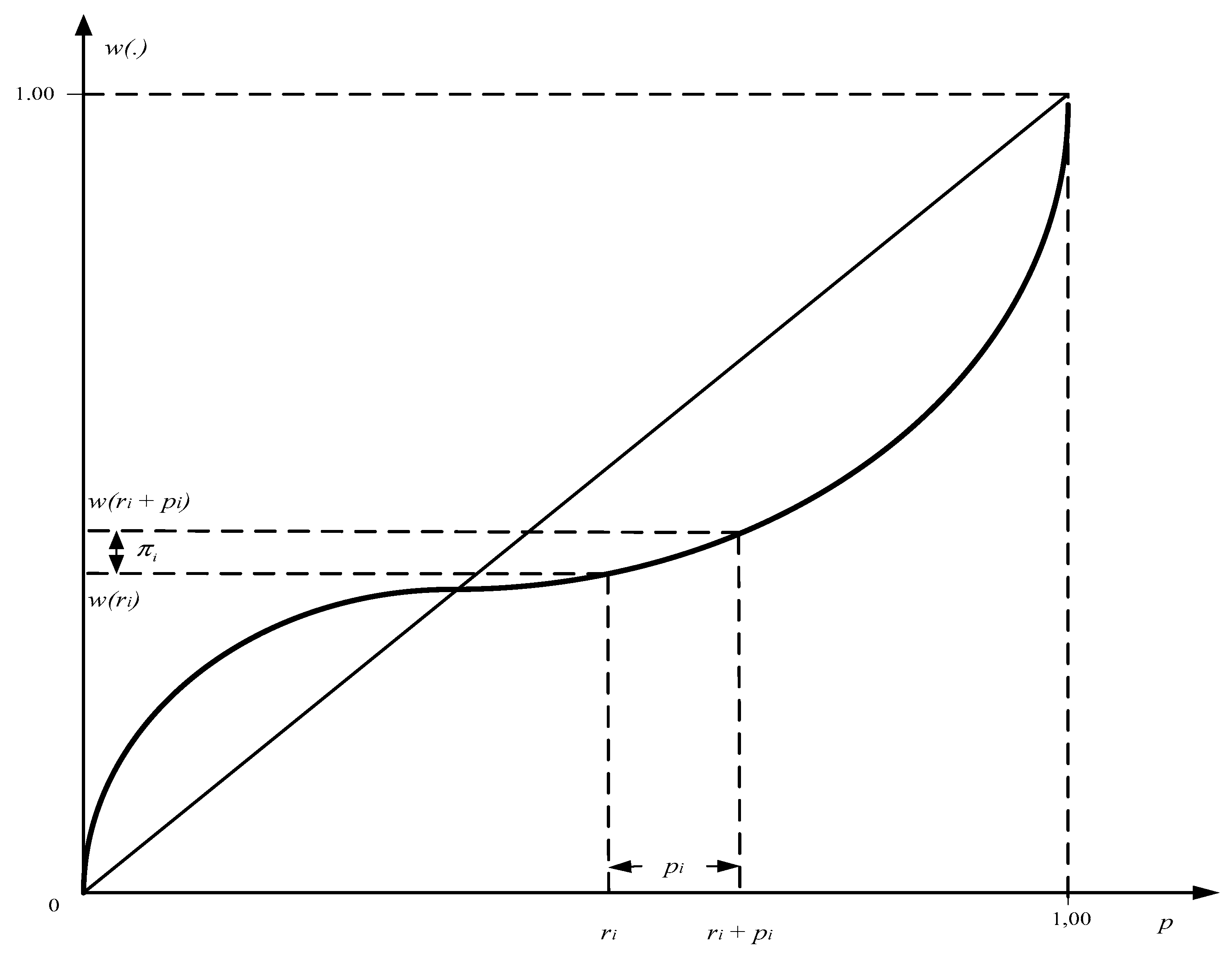
In the theory of rank-dependent utility, the relationship between the decision weights and the probabilities of the corresponding outcomes is quite complex. To clarify this relationship, let us turn to Figure 3 (the idea of the figure is borrowed from (Wakker 2010)).

In this figure, the point $r_i$ schematically represents the rank of the $i\text{-}\mathrm{th}$ outcome on the probability scale. The point $r_i+p_i$ schematically represents the sum of the rank $r_i$ and the probability of the realization of $i\text{-}\mathrm{th}$ outcome $p_i$. Using the graph of the probability weighting function $w(p)$, on the vertical scale of the weights, we determine the values $w\left(r_i\right)$, $w\left(r_i+p_i\right)$, corresponding to the points $r_i$ and $r_i+p_i$.

The decision weight of the $i\text{-}\mathrm{th}$ outcome is determined as

$${\pi }_i=\pi \left(p_i\right)=w\left(r_i+p_i\right)$$

(9)

Let’s assume, there is a prospect $A=\left(x_1,p_1,\dots ,x_n,p_n\right)$, $x_1>x_2>\dots >x_n$. For each $i\text{-}\mathrm{th}$ outcome, $i=1,\dots ,n$, their estimates are known in the utility scale $u\left(k_i\right)$, and the decision weight ${\pi }_i$, as determined by expression (9). Then, the weighted value of the rank-dependent utility for this prospect is calculated by the expression

$$U_{RD}\left(A\right)={\displaystyle \sum _{i=1}^{n}u\left(k_i\right){\pi }_i={\displaystyle \sum _{i=1}^{n}u\left(k_i\right)}}\left[w\left(p_i+\dots +p_n\right)-w\left(p_{i-1}+\dots +p_1\right)\right]$$

(10)

4. Cumulative Prospect Theory

The prospect theory is currently the most advanced descriptive theory of prospect selection. The first version of the theory was presented in (Kahneman and Tversky 1979). This version in scientific literature is usually called the original prospect theory. The cumulative prospect theory was presented in (Tversky and Kahneman 1992). It is a significant extension of the original prospect theory. This theory combines the principles of expected utility theory, probability weighting, and rank-dependent utility.

The authors in their theory propose to use the following parameterized form of the value function:

$$\begin{gathered} fork>0v(k)=k^{\theta }; \\ fork=0v(k)=0; \\ fork<0v(k)=-\lambda {(k)}^{{\theta }^{\prime }}, \end{gathered}$$

(11)

where $k$—the value of the evaluation criterion; $\theta ,{\theta }^{\prime }$—function parameters; $\lambda$—parameter characterizing loss aversion. The authors suggest using the value $\lambda =2.25$.

Note that the concept of a value function in this context is fully consistent with the concept of a utility function in expected utility theory.

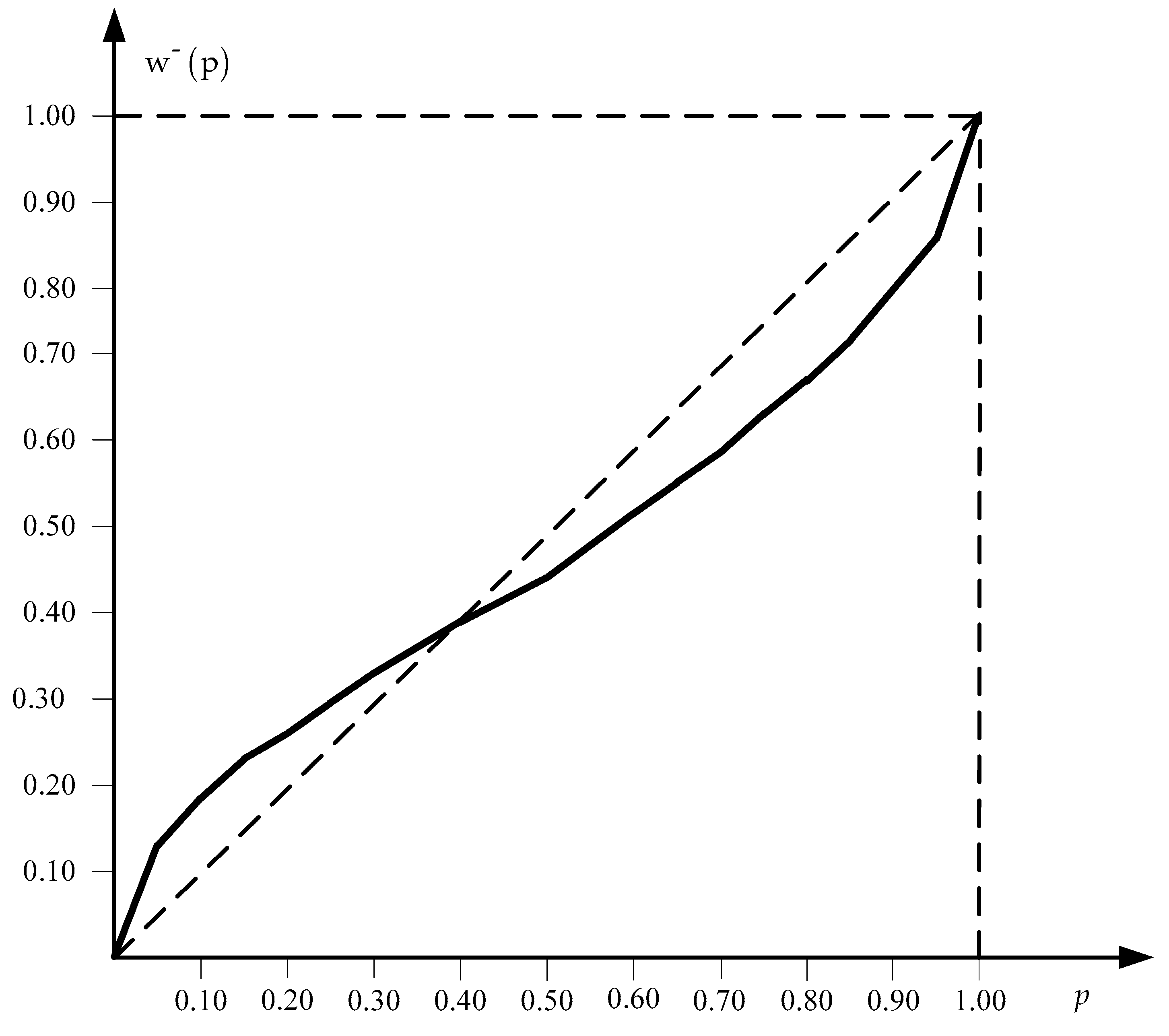
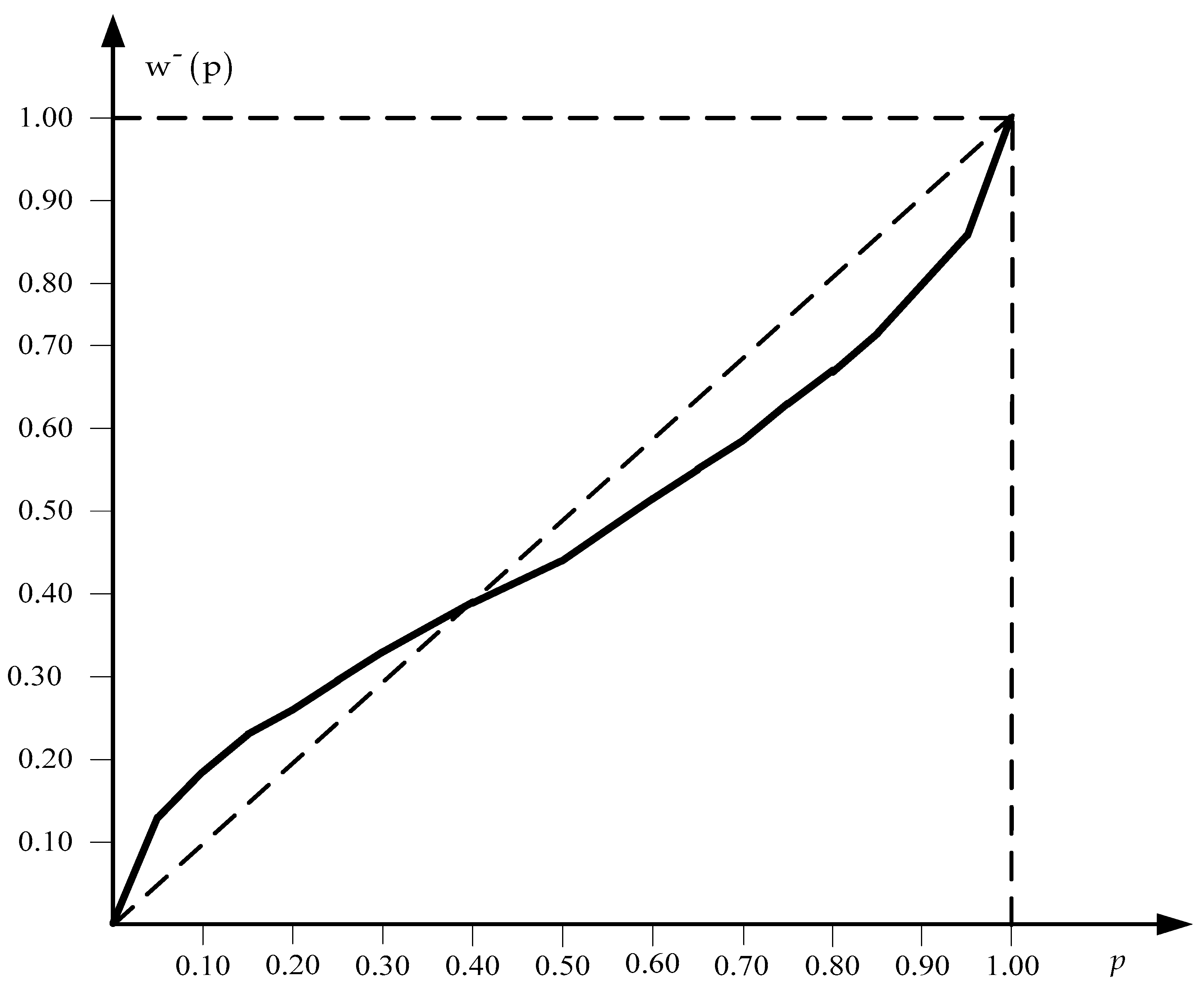
The authors propose to use the following probability weighting functions for outcomes’ probabilities with positive and negative estimates:

$$w^{+}(p)=\frac{p^{\gamma }}{{\left(p^{\gamma }+{\left(1-p\right)}^{\gamma }\right)}^{\frac{1}{\gamma }}},\gamma =0.61.$$

(12)

$$w^{-}(p)=\frac{p^{\sigma }}{{\left(p^{\sigma }+{\left(1-p\right)}^{\sigma }\right)}^{\frac{1}{\sigma }}},\sigma =0.69.$$

(13)

The graphs of these functions are shown in Figure 4.

How can the generalized value of the prospect be calculated within the framework of the cumulative prospect theory? Let a prospect $A=\left(k_1,p_1,\dots ,k_n,p_n\right)$ be given, the outcomes of which are regulated in a decreasing order of their estimates:

$$k_1\ge k_2\ge \dots \ge k_r\ge 0\ge k_{r+1}\ge k_{r+2}\ge \dots \ge k_n$$

(14)

Note that compared to the rank-dependent utility theory, this theory allows negative outcome estimates.

Using the probabilities’ weighting functions $w^{+}(p)$, $w^{-}(p)$, and the values of the outcomes’ probabilities, the decision weights’ values for the outcomes are calculated by the expressions:

$$fori\le r{\pi }_i^{+}=w^{+}\left(p_i+\dots +p_1\right)-w^{+}\left(p_{i-1}+\dots +p_1\right),{\pi }_1^{+}=w^{+}\left(p_1\right);$$

(15)

$$forj>r{\pi }_j^{-}=w^{-}\left(p_j+\dots +p_n\right)-w^{-}\left(p_{j+1}+\dots +p_n\right),{\pi }_n^{-}=w^{-}\left(p_n\right).$$

(16)

Then the generalized value of prospect A value is calculated by the expression

$$V_{PT}\left(A\right)={\displaystyle \sum _{i=1}^{r}v\left(k_i\right)}{\pi }_i^{+}+{\displaystyle \sum _{j=i+1}^{n}v\left(k_j\right){\pi }_j^{-}},$$

(17)

where ${\pi }_i^{+}$ is the decision weight of the $i\text{-}\mathrm{th}$ outcome with a positive estimate, calculated by expression (15);

${\pi }_j^{-}$ is the decision weight of the $j\text{-}\mathrm{th}$ outcome with a negative estimate, calculated by expression (16);

$v\left(k_i\right)$, $v\left(k_j\right)$—estimate of the $i\text{-}\mathrm{th}$ and $j\text{-}\mathrm{th}$ outcome values, respectively.

5. Cumulative Prospect Theory’s Version with Fuzzy Outcome Estimates

The fuzzy sets theory’s basics were laid in the paper by Zadeh (1965). A fuzzy number is a fuzzy set, which is defined on a real number set. At present, the theory of fuzzy sets has a very widespread application in various fields of human activity (Klir and Yuan 1995; Chen and Ku 2008; Dutta and Dash 2018; Zimmermann 2001; Gupta and Ragade 1977; Singh et al. 2013).

In general, the membership function graph of a fuzzy number can form an arbitrary shape, which satisfies the following restrictions: any fuzzy number is a convex fuzzy set with a membership function, whose membership values are strictly monotonically increasing than strictly monotonically decreasing with increasing values on the used quantitative scale. Additionally, L-functions are possible, whose membership values are strictly monotonically increasing or strictly monotonically decreasing with increasing values on the used quantitative scale. The most common fuzzy numbers have membership functions with graphs of triangular and trapezoidal shapes.

In the present paper, to model the uncertainties associated with the outcome estimates, normal triangular fuzzy numbers are used (the maximum value of the membership function equals 1); however, all subsequent interpretations and conclusions will also be valid for normal trapezoidal fuzzy numbers. The use of generalized fuzzy numbers, as well as intuitionistic fuzzy number and fuzzy number type 2 have been considered inappropriate for the purposes of this paper.

The choice of the optimal perspective in the proposed version of the fuzzy prospect theory is based on the comparison of the resulting fuzzy estimates. Numerous methods have been proposed for comparing fuzzy numbers. These methods can be divided into the following general groups:

• A group of methods that use the distance values from the centroids of fuzzy numbers to certain original points (Wang et al. 2006; Cheng 1998).
• A group of methods that use the specific areas as an evaluation function (Rao and Shankar 2012; Wang and Lee 2008).
• A group of methods that use the concepts of maximum and minimum values (Chou et al. 2011).

A specific method for comparing fuzzy numbers is presented in (Ganesh and Jayakumar 2014).

Other methods for comparing fuzzy numbers are also offered. Using the appropriate method allows estimating the distances between the fuzzy numbers at any of their relative position on the measurement scale.

Theoretical basics for a simple comparison of fuzzy numbers can be found in (Buckley 2006).

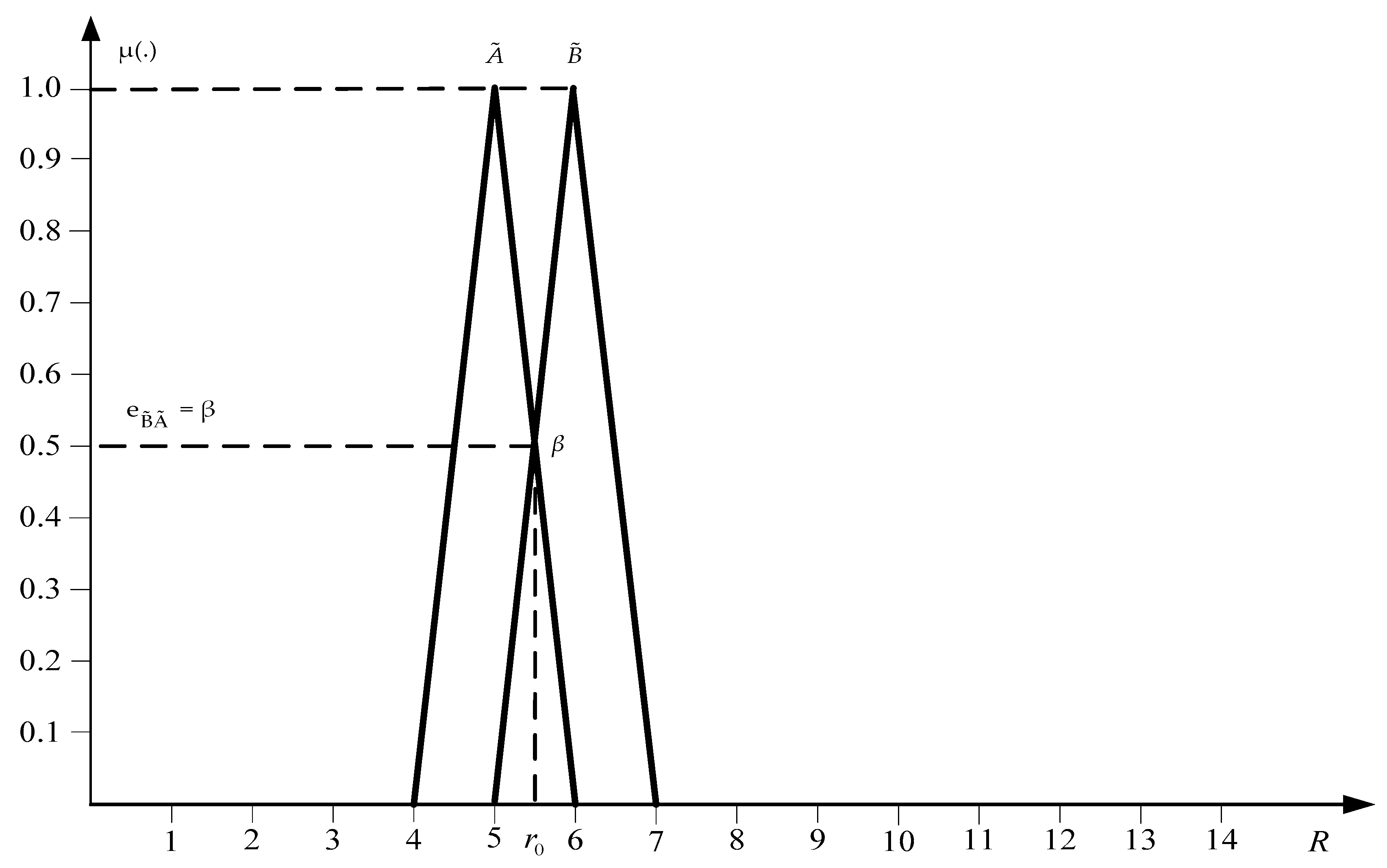
In this paper, we use a simple method, the essence of which is as follows. Let’s turn to Figure 5.

This figure graphically represents two fuzzy numbers $\tilde{A}$ and $\tilde{B}$. It is necessary to determine which of these fuzzy numbers is greater. For this, two estimated values are calculated: $e_{\tilde{A}\tilde{B}}$, $e_{\tilde{B}\tilde{A}}$. The value $e_{\tilde{B}\tilde{A}}$ is calculated by the expression

$$e_{\tilde{B}\tilde{A}}=ma{x}_{p>r}\left\{min\left({\mu }_{\tilde{A}}(p)\right),{\mu }_{\tilde{B}}(r)\right\},p,r\in R.$$

(18)

Expression (18) sets the requirement of what core of fuzzy number $\tilde{B}$ should settle to the right of fuzzy number $\tilde{A}$’s core.

Obviously, $e_{\tilde{B}\tilde{A}}=1$ for fuzzy numbers, $\tilde{A}$ and $\tilde{B}$, in Figure 5. This value is reached at a point $r_0=6$.

The value $e_{\tilde{A}\tilde{B}}$ is defined as the value of the membership function for the point $\beta$, at which the graphs of the membership functions $\mu \left(\tilde{A}\right)$, $\mu \left(\tilde{B}\right)$ intersect. The number $\beta$ is interpreted as the degree to which $\tilde{A}$ is greater than $\tilde{B}$ (Buckley 2006, pp. 17–18). The fuzzy number $\tilde{B}$ is greater than the fuzzy number $\tilde{A}$ to the degree $\beta$ if

$$\tilde{B}>\tilde{A}\to e_{\tilde{B}\tilde{A}}=1,e_{\tilde{A}\tilde{B}}\le \beta .$$

(19)

Value of $\beta$ is assessed subjectively. In this paper, $\beta =0.5$ as a compromise.

Cumulative prospect theory is designed to select optimal prospects when the initial data are presented in a clear deterministic form. However, in real circumstances, it is not always possible to provide deterministic estimates of outcomes. Interval or fuzzy estimates can be used to model the existing uncertainty. This paper presents a version of the cumulative prospect theory with fuzzy outcome estimates.

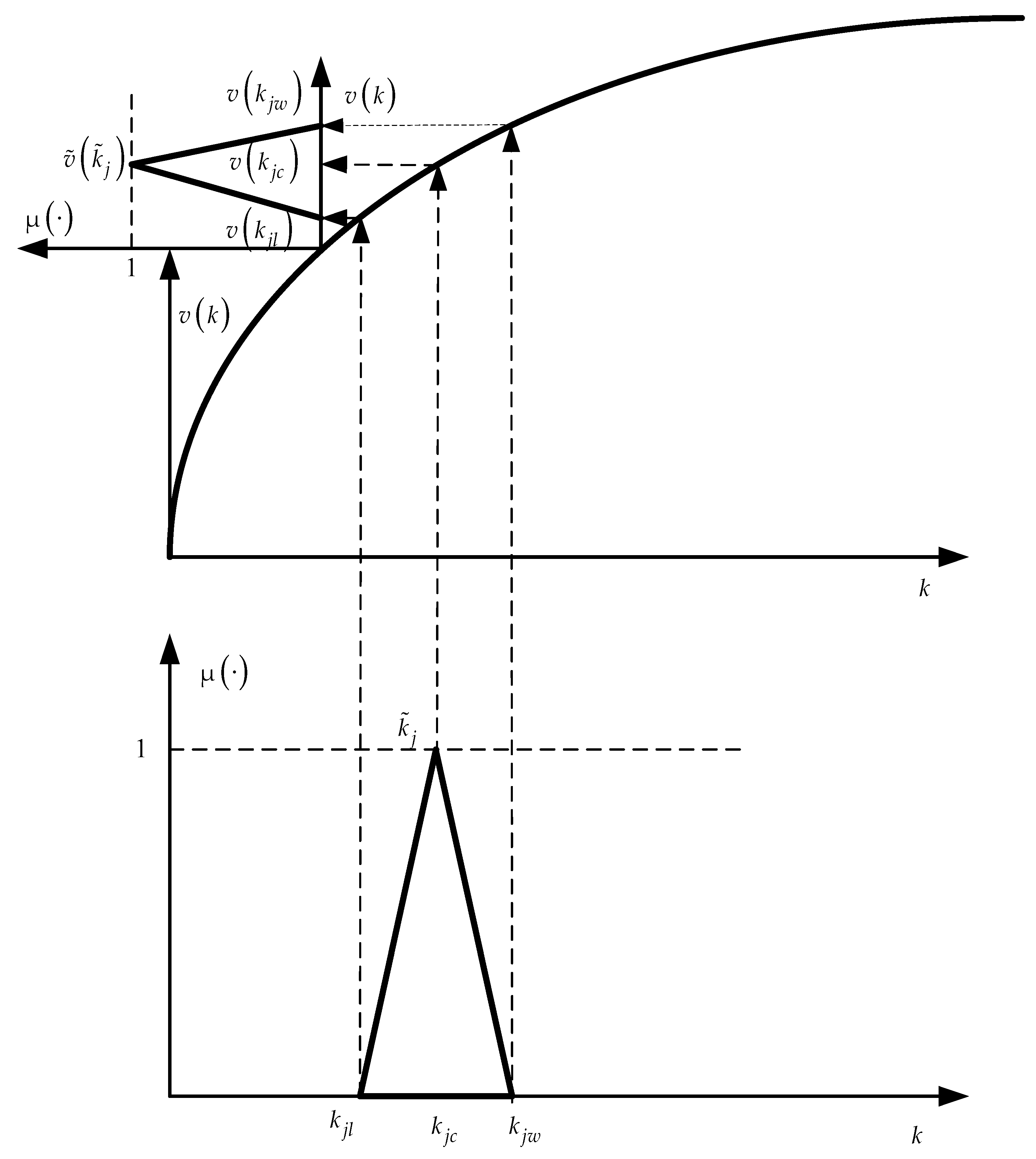
Let the outcome estimates be given in the form of fuzzy numbers ${\tilde{k}}_j=\left(k_{jl},k_{jc},k_{jw}\right)$, $j=1,\dots ,n$, where $k_{jl}$ is the lower limit of the fuzzy number ${\tilde{k}}_j$ support, $k_{jc}$ is the value of the estimate corresponding to the membership function value $\mu \left({\tilde{k}}_j\right)=1$, $k_{jw}$ is the upper limit of the fuzzy number ${\tilde{k}}_j$ support. A fuzzy outcomes’ estimates should satisfy the following requirements: (a) minimal lower bound for any positive fuzzy number is greater or equal to 0; (b) maximal right bound for any negative fuzzy number is smaller or equal to 0. Fuzzy numbers (−a, 0, 0), (0, 0, b) are also possible, where $a$ is the left support boundary and $b$ is the right support boundary for the corresponding fuzzy number.

As the cumulative prospect theory uses value estimates instead of outcome estimates, we must transform fuzzy estimates ${\tilde{k}}_j$ into fuzzy estimates $\tilde{v}\left({\tilde{k}}_j\right)$. The scheme of such a transformation for a positive fuzzy value ${\tilde{k}}_j$ is shown in Figure 6. This transformation is based on the extension principle formulated in (Zadeh 1965) and developed in subsequent works by the author. For negative values of outcome estimates, their transformation is performed in exactly the same way.

Using the given fuzzy number ${\tilde{k}}_j$ and the graph of the function $v\left(k\right)$, we define the characteristic points $v\left(k_{jl}\right)$, $v\left(k_{jc}\right)$, $v\left(k_{jw}\right)$ and the corresponding fuzzy number $\tilde{v}\left({\tilde{k}}_j\right)$. In exactly the same way, fuzzy value estimates for other prospect outcomes are determined.

Then the fuzzy value of the generalized value for prospect A can be calculated by the expression

$${\tilde{V}}_{PT}\left(A\right)={\displaystyle \sum _{i=1}^r\tilde{v}\left({\tilde{k}}_i\right)}{\pi }_i^{+}+{\displaystyle \sum _{j=r+1}^n\tilde{v}\left({\tilde{k}}_j\right){\pi }_j^{-}},$$

(20)

Where ${\pi }_i^{+}$—the decision weight of the $i\text{-}\mathrm{th}$ outcome with a positive estimate, calculated by expression (15);

${\pi }_j^{-}$—the decision weight of the $j\text{-}\mathrm{th}$ outcome with a negative estimate, calculated by expression (16);

$\tilde{v}\left({\tilde{k}}_i\right)$, $\tilde{v}\left({\tilde{k}}_j\right)$—fuzzy estimates of the value of the $i\text{-}\mathrm{th}$ and $j\text{-}\mathrm{th}$ outcomes.

6. Illustrative Example

There are two prospects: A and B (see Figure 7).

The value function is given in the form $v\left(k\right)=k^{0.05}$, $k>0$, $v\left(k\right)=-2.25\left(v\left(k\right)\right)$. The probability weighting functions are given by expressions (12), (13). It is necessary to choose the optimal prospect based on the generalized fuzzy estimate (18).

Using the above expressions for the value function, we calculate fuzzy estimates of the prospects’ outcome values:

Prospect A:	Prospect B:
$\tilde{v}(1)=(1.232,1.237,1.241)$	$\tilde{v}\left(1\right)=\left(1.222,1.227,1.232\right)$
$\tilde{v}\left(2\right)=\left(1.210,1.216,1.222\right)$	$\tilde{v}\left(2\right)=\left(1.195,1.203,1.210\right)$
$\tilde{v}\left(3\right)=\left(1.194,1.203,1.210\right)$	$\tilde{v}\left(3\right)=\left(1.175,1.185,1.195\right)$
$v\left(4\right)=\left(-2.644,-2.614,-2.576\right)$	$\tilde{v}\left(4\right)=\left(-2.576,-2.524,-2.439\right)$
$\tilde{v}\left(5\right)=\left(-2.689,-2.666,-2.644\right)$	$\tilde{v}\left(5\right)=\left(-2.643,-2.614,-2.576\right)$
$\tilde{v}\left(6\right)=\left(-2.722,-2.704,-2.686\right)$	$\tilde{v}\left(6\right)=\left(-2.772,-2.706,-2.688\right)$

Using expressions (15), (16), we calculate the values of the decision weights. When calculating the decision weights, the weights of the relevant probabilities are calculated using expressions (12), (13).

- prospect A:

$${\pi }_1^{+}=w^{+}\left(p_1\right)=w^{+}\left(0.10\right)=0.185;$$

$$\begin{gathered} {\pi }_2^{+}=w^{+}\left(p_1+p_2\right)-w^{+}\left(p_1\right)=w^{+}\left(0.10+0.20\right)-w^{-}\left(0.10\right)= \\ =w^{+}\left(0, 30\right)-w^{+}\left(0, 10\right)=0.318-0.185=0.133; \end{gathered}$$

$$\begin{gathered} {\pi }_3^{+}=w^{+}\left(p_1+p_2+p_3\right)-w^{+}\left(p_1+p_2\right)=w^{+}\left(0.10+0.20+0.20\right)-w^{+}\left(0.10+0.20\right)= \\ =w^{+}\left(0.50\right)-w^{+}\left(0.30\right)=0.421-0.318=0.103; \end{gathered}$$

$$\begin{gathered} {\pi }_4^{-}=w^{-}\left(p_4+p_5+p_6\right)-w^{-}\left(p_5+p_6\right)=w^{-}\left(0.30+0.10+0.10\right)-w^{-}\left(0.10+0.10\right)= \\ =w^{-}\left(0.50\right)-w^{-}\left(0.20\right)=0.453-0.257=0.196; \end{gathered}$$

$$\begin{gathered} {\pi }_5^{-}=w^{-}\left(p_5+p_6\right)-w^{-}\left(p_6\right)=w^{-}\left(0.10+0.10\right)-w^{-}\left(0.10\right)= \\ =w^{-}\left(0.20\right)-w^{-}\left(0.10\right)=0.257-0.170=0.087; \end{gathered}$$

$${\pi }_6^{-}=w^{-}\left(p_6\right)=w^{-}\left(0.10\right)=0.170.$$

- prospect B:

$${\pi }_1^{+}=w^{+}\left(p_1\right)=w^{+}\left(0.20\right)=0.261;$$

$$\begin{gathered} {\pi }_2^{+}=w^{+}\left(p_1+p_2\right)-w^{+}\left(p_1\right)=w^{+}\left(0.20+0.20\right)-w^{-}\left(0.20\right)= \\ =w^{+}\left(0.40\right)-w^{+}\left(0.20\right)=0.370-0.261=0.109; \end{gathered}$$

$$\begin{gathered} {\pi }_3^{+}=w^{+}\left(p_1+p_2+p_3\right)-w^{+}\left(p_1+p_2\right)=w^{+}\left(0.20+0.20+0.10\right)-w^{+}\left(0.20+0.20\right)= \\ =w^{+}\left(0.50\right)-w^{+}\left(0.40\right)=0.421-0.370=0.051; \end{gathered}$$

$$\begin{gathered} {\pi }_4^{-}=w^{-}\left(p_4+p_5+p_6\right)-w^{-}\left(p_5+p_6\right)=w^{-}\left(0.20+0.20+0.10\right)-w^{-}\left(0.20+0.10\right)= \\ =w^{-}\left(0.50\right)-w^{-}\left(0.30\right)=0.453-0.327=0.126; \end{gathered}$$

$$\begin{gathered} {\pi }_5^{-}=w^{-}\left(p_5+p_6\right)-w^{-}\left(p_6\right)=w^{-}\left(0.20+0.10\right)-w^{-}\left(0.10\right)= \\ =w^{-}\left(0.30\right)-w^{-}\left(0.10\right)=0.327-0.170=0.157; \end{gathered}$$

$${\pi }_6^{-}=w^{-}\left(p_6\right)=w^{-}\left(0.10\right)=0.170.$$

Using expression (18) we calculate the generalized fuzzy value estimates for both prospects.

$$\begin{array}{l}{\tilde{V}}_{PT}\left(A\right)=\left(1.232,1.237,1.241\right)*0.185+\left(1.210,1.216,1.222\right)*0.133+\\ +\left(1.194,1.203,1.210\right)*0.103-+\left(-2.644,-2.614,-2.576\right)*0.196-\\ +\left(-2.689,-2.666,-2.644\right)*0.087+\left(-2.722,-2.704,-2.666\right)*0.17=\\ =\left(0.548,0.553,0.556\right)-\left(1.215,1.205,1.192\right)=\left(-0.667,-0.652,-0.636\right).\end{array}$$

$$\begin{array}{l}{\tilde{V}}_{PT}\left(B\right)=\left(1.222,1.227,1.232\right)*0.261+\left(1.195,1.203,1.210\right)*0.109+\\ +\left(1.175,1.185,1.195\right)*0.051+\left(-2.576,-2.524,-2.435\right)*0.126-\\ +\left(-2.643,-2.614,-2.576\right)*0.157+\left(-2.722,-2.706,-2.686\right)*0.170=\\ \left(0.509,0.512,0.516\right)-\left(1.203,1.189,1.168\right)=\left(-0.694,-0.577,-0.652\right).\end{array}$$

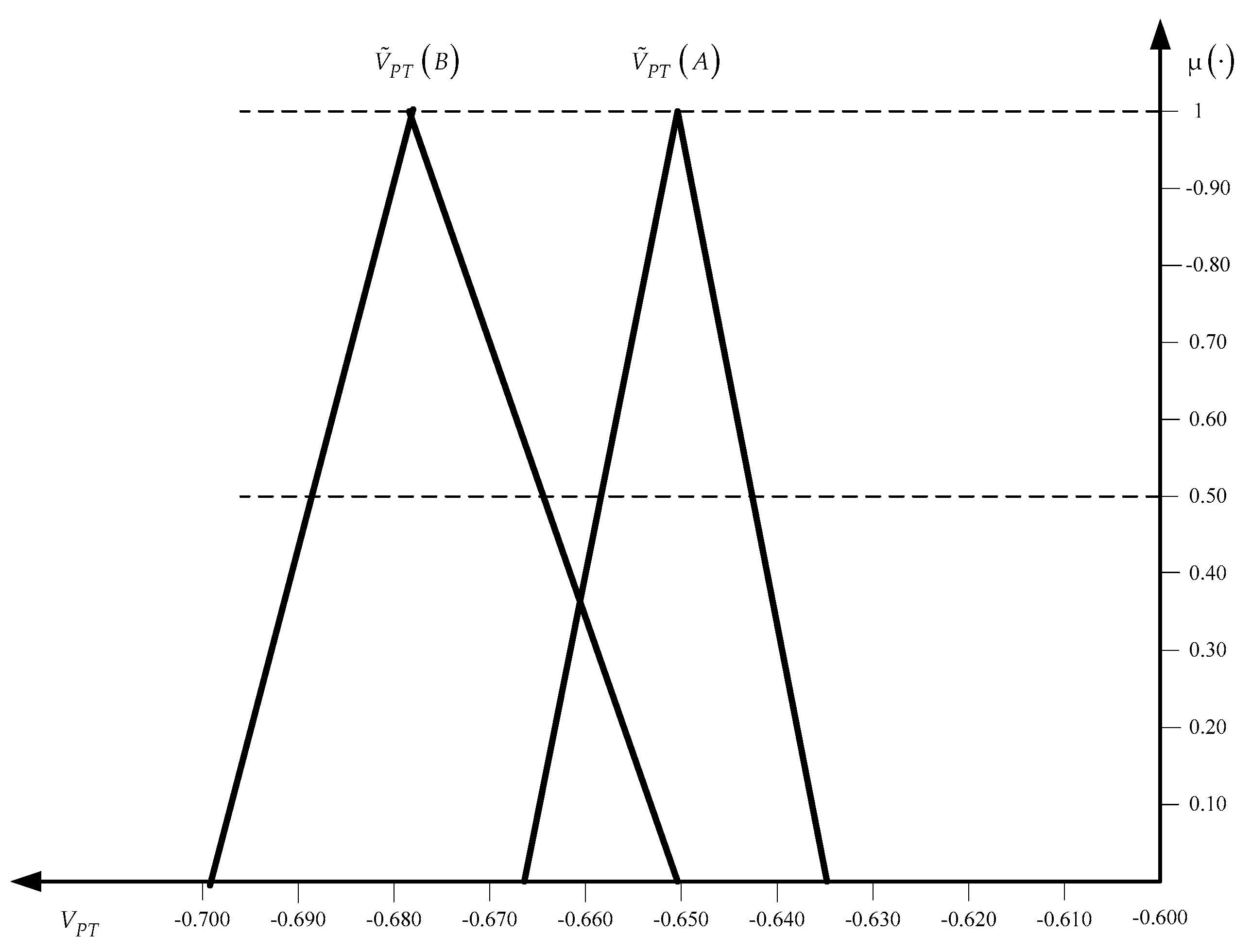
To choose the optimal prospect, it is necessary to compare the fuzzy numbers ${\tilde{V}}_{PT}\left(A\right)$, ${\tilde{V}}_{PT}\left(B\right)$.

In Figure 8, the graphs of the membership functions of the fuzzy numbers ${\tilde{V}}_{PT}\left(A\right)$, ${\tilde{V}}_{PT}\left(B\right)$ are presented.

Using the above approach to compare fuzzy numbers, it can be unambiguously concluded that prospect A is optimal.

It should be noted that fuzzy value estimates are always asymmetrical; hence, the resulting fuzzy estimates are also always asymmetrical. It allows a reliable comparison to be implemented.

7. Conclusions

The expected utility theory (von Neuman and Morgenstern 1947) has made a significant contribution to the development of effective methods for choosing decisions under risk and uncertainty. In subsequent years, this theory has evolved, with the end result of a cumulative prospect theory. Why could the expected utility theory not satisfy decision-makers? The fact is that the attitude of decision-makers (DM) towards risk is the most important factor in choosing the best decisions in the face of risk and uncertainty. In the expected utility theory, the risk attitude of DM is modeled only in the form of the utility function. Practical research has shown that in addition to possible losses, many other factors affect the attitude to risk. Taking these factors into account led to the development of extensions of the expected utility theory. In the probability weighting approach, the attitude to the risk of loss is modeled in the form of the utility function. Additionally, using the probability weighting function, the attitude of DM to risk is modeled on the set of outcome probabilities. In the theory of rank-dependent utility, using decision weights, the attitude to risk of DM is modeled on a set of estimates of the prospect’s outcomes.

In this paper, we have devoted a significant amount to describing the predecessors of the prospect theory. This is because without understanding the previous extensions, it is impossible to understand and explain the prospect theory.

The prospect theory, in its most advanced form, includes everything accumulated by previous versions regarding the modeling of DM risk attitudes. The modern form of the cumulative prospect theory is based on numerous psychological studies by the authors (Kahneman 2002), (Kahneman and Tversky 1984), (Kahneman et al. 1991), (Kahneman et al. 2008), (Tversky and Kahneman 1974, 1981, 1986, 1991). Therefore, the theory handles all risk factors correctly. The authors proposed their own version of the probability weighting function, which is widely used in by decision analysts. Their proposed parametric forms of value functions for the estimates of prospect’s positive and negative outcomes have also received overall recognition. The theory includes the concepts of decision weights, first formulated in the theory of rank-dependent utility.

For many approaches to choosing a decision, their fuzzy versions are presented. This is especially true for multi-criteria approaches to the decision choice. There is a version of the fuzzy expected utility theory where the utility function is not formed, but the utility is presented in the form of fuzzy categories, which are then used to calculate the expected utility of the alternatives.

This approach is inapplicable to the prospect theory since its value functions have a parametric form. Therefore, in this paper, a version of the prospect theory is proposed, provided that the outcomes’ estimates are given in a fuzzy form. Such estimates can be used in situations where it is impossible to set deterministic estimates for various reasons.

The transformation of fuzzy estimates into fuzzy estimates of values is carried out based on the value functions. Figure 6 shows a graphical interpretation of this transformation. However, in practice, the definition of fuzzy values’ estimates is performed by calculating the characteristic points of fuzzy numbers $\tilde{v}\left({\tilde{k}}_j\right)$, using the characteristic values of fuzzy estimates ${\tilde{k}}_j$ and analytical expressions of value functions (11). This transformation is based on the extension principle of L.A. Zadeh (Zadeh 1965) and is a variant of fuzzy functions, the components of which are fuzzy numbers.

Let us analyze the results obtained in this work. First, the results of transformation show that negative fuzzy values prevail. This is exclusively related to the nature of the value functions (11). In prospect theory, the negative values’ estimates play a more important role than their positive estimates. This is a reflection of the loss aversion in individuals. To choose the optimal prospect, such asymmetry of fuzzy estimates is not of importance. In the above illustrated example, both generalized fuzzy estimates are negative, which did not affect the choice of the optimal prospect.

Fuzzy value estimates are robust estimates. Otherwise, the degree of fuzziness of the initial estimates has little effect on the degree of fuzziness of the resulting fuzzy value estimates. This fact is a positive characteristic of the proposed version.