Modelling Volatile Time Series with V-Transforms and Copulas

Abstract

An approach to the modelling of volatile time series using a class of uniformity-preserving transforms for uniform random variables is proposed. V-transforms describe the relationship between quantiles of the stationary distribution of the time series and quantiles of the distribution of a predictable volatility proxy variable. They can be represented as copulas and permit the formulation and estimation of models that combine arbitrary marginal distributions with copula processes for the dynamics of the volatility proxy. The idea is illustrated using a Gaussian ARMA copula process and the resulting model is shown to replicate many of the stylized facts of financial return series and to facilitate the calculation of marginal and conditional characteristics of the model including quantile measures of risk. Estimation is carried out by adapting the exact maximum likelihood approach to the estimation of ARMA processes, and the model is shown to be competitive with standard GARCH in an empirical application to Bitcoin return data.

1. Introduction

In this paper, we show that a class of uniformity-preserving transformations for uniform random variables can facilitate the application of copula modelling to time series exhibiting the serial dependence characteristics that are typical of volatile financial return data. Our main aims are twofold: to establish the fundamental properties of v-transforms and show that they are a natural fit to the volatility modelling problem; to develop a class of processes using the implied copula process of a Gaussian ARMA model that can serve as an archetype for copula models using v-transforms. Although the existing literature on volatility modelling in econometrics is vast, the models we propose have some attractive features. In particular, as copula-based models, they allow the separation of marginal and serial dependence behaviour in the construction and estimation of models.

A distinction is commonly made between genuine stochastic volatility models, as investigated by Taylor (1994) and Andersen (1994), and GARCH-type models as developed in a long series of papers by Engle (1982), Bollerslev (1986), Ding et al. (1993), Glosten et al. (1993) and Bollerslev et al. (1994), among others. In the former an unobservable process describes the volatility at any time point while in the latter volatility is modelled as a function of observable information describing the past behaviour of the process; see also the review articles by Shephard (1996) and Andersen and Benzoni (2009). The generalized autoregressive score (GAS) models of Creal et al. (2013) generalize the observation-driven approach of GARCH models by using the score function of the conditional density to model time variation in key parameters of the time series model. The models of this paper have more in common with the observation-driven approach of GARCH and GAS but have some important differences.

In GARCH-type models, the marginal distribution of a stationary process is inextricably linked to the dynamics of the process as well as the conditional or innovation distribution; in most cases, it has no simple closed form. For example, the standard GARCH mechanism serves to create power-law behaviour in the marginal distribution, even when the innovations come from a lighter-tailed distribution such as Gaussian (Mikosch and Stărică 2000). While such models work well for many return series, they may not be sufficiently flexible to describe all possible combinations of marginal and serial dependence behaviour encountered in applications. In the empirical example of this paper, which relates to log-returns on the Bitcoin price series, the data appear to favour a marginal distribution with sub-exponential tails that are lighter than power tails and this cannot be well captured by standard GARCH models. Moreover, in contrast to much of the GARCH literature, the models we propose make no assumptions about the existence of second-order moments and could also be applied to very heavy-tailed situations where variance-based methods fail.

Let $X_1,\dots ,X_n$ be a time series of financial returns sampled at (say) daily frequency and assume that these are modelled by a strictly stationary stochastic process $\left(X_t\right)$ with marginal distribution function (cdf) $F_X$. To match the stylized facts of financial return data described, for example, by Campbell et al. (1997) and Cont (2001), it is generally agreed that $\left(X_t\right)$ should have limited serial correlation, but the squared or absolute processes $\left(X_t^2\right)$ and $\left(\right|X_t\left|\right)$ should have significant and persistent positive serial correlation to describe the effects of volatility clustering.

In this paper, we refer to transformed series like $\left(\right|X_t\left|\right)$, in which volatility is revealed through serial correlation, as volatility proxy series. More generally, a volatility proxy series $\left(T\left(X_t\right)\right)$ is obtained by applying a transformation $T:\mathbb{R}\mapsto \mathbb{R}$ which (i) depends on a change point ${\mu }_T$ that may be zero, (ii) is increasing in $X_t-{\mu }_T$ for $X_t\ge {\mu }_T$ and (iii) is increasing in ${\mu }_T-X_t$ for $X_t\le {\mu }_T$.

Our approach in this paper is to model the probability-integral transform (PIT) series $\left(V_t\right)$ of a volatility proxy series. This is defined by $V_t=F_{T\left(X\right)}\left(T\left(X_t\right)\right)$ for all t, where $F_{T\left(X\right)}$ denotes the cdf of $T\left(X_t\right)$. If $\left(U_t\right)$ is the PIT series of the original process $\left(X_t\right)$, defined by $U_t=F_X\left(X_t\right)$ for all t, then a v-transform is a function describing the relationship between the terms of $\left(V_t\right)$ and the terms of $\left(U_t\right)$. Equivalently, a v-transform describes the relationship between quantiles of the distribution of $X_t$ and the distribution of the volatility proxy $T\left(X_t\right)$. Alternatively, it characterizes the dependence structure or copula of the pair of variables $(X_t,T\left(X_t\right))$. In this paper, we show how to derive flexible, parametric families of v-transforms for practical modelling purposes.

To gain insight into the typical form of a v-transform, let $x_1,\dots ,x_n$ represent the realized data values and let $u_1,\dots ,u_n$ and $v_1,\dots ,v_n$ be the samples obtained by applying the transformations $v_t=F_n^{\left(\right|X\left|\right)}\left(\right|x_t\left|\right)$ and $u_t=F_n^{\left(X\right)}\left(x_t\right)$, where $F_n^{\left(X\right)}\left(x\right)=\frac{1}{n+1}{\sum }_{t=1}^n{I}_{\{x_t\le x\}}$ and $F_n^{\left(\right|X\left|\right)}\left(x\right)=\frac{1}{n+1}{\sum }_{t=1}^n{I}_{\left\{\right|x_t|\le x\}}$ denote scaled versions of the empirical distribution functions of the $x_t$ and $|x_t|$ samples, respectively. The graph of $(u_t,v_t)$ gives an empirical estimate of the v-transform for the random variables $(X_t,|X_t\left|\right)$. 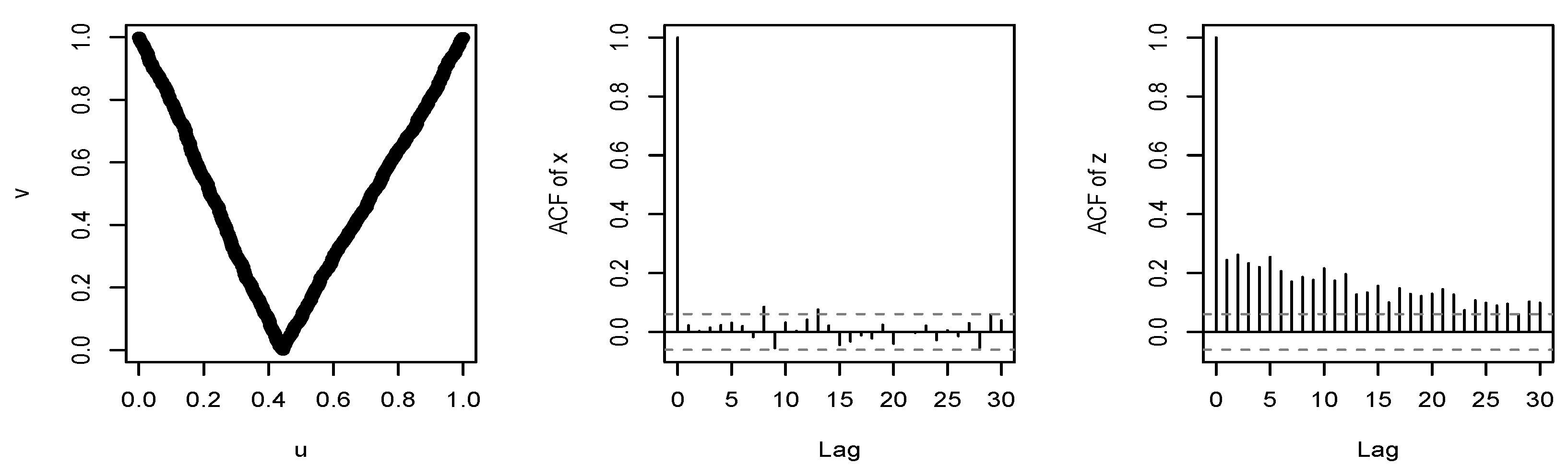In the left-hand plot of Figure 1 we show the relationship for a sample of $n=1043$ daily log-returns of the Bitcoin price series for the years 2016–2019. Note how the empirical v-transform takes the form of a slightly asymmetric ‘V’.

Figure 1. Scatterplot of $v_t$ against $u_t$ (left), sample acf of raw data $x_t$ (centre) and sample acf of $z_t={\Phi }^{-1}\left(v_t\right)$ (right). The transformed data are defined by $v_t=F_n^{\left(\right|X\left|\right)}\left(\right|x_t\left|\right)$ and $u_t=F_n^{\left(X\right)}\left(x_t\right)$ where $F_n^{\left(X\right)}$ and $F_n^{\left(\right|X\left|\right)}$ denote versions of the empirical distribution function of the $x_t$ and $|x_t|$ values, respectively. The sample size is $n=1043$ and the data are daily log-returns of the Bitcoin price for the years 2016–2019.

The right-hand plot of Figure 1 shows the sample autocorrelation function (acf) of the data given by $z_t={\Phi }^{-1}\left(v_t\right)$ where $\Phi$ is the standard normal cdf. This reveals a persistent pattern of positive serial correlation which can be modelled by the implied ARMA copula. This pattern is not evident in the acf of the raw $x_t$ data in the centre plot.

To construct a volatility model for $\left(X_t\right)$ using v-transforms, we need to specify a process for $\left(V_t\right)$. In principle, any model for a series of serially dependent uniform variables can be applied to $\left(V_t\right)$. In this paper, we illustrate concepts using the Gaussian copula model implied by the standard ARMA dependence structure. This model is particularly tractable and allows us to derive model properties and fit models to data relatively easily.

There is a large literature on copula models for time series; see, for example, the review papers by Patton (2012) and Fan and Patton (2014). While the main focus of this literature has been on cross-sectional dependencies between series, there is a growing literature on models of serial dependence. First-order Markov copula models have been investigated by Chen and Fan (2006), Chen et al. (2009) and Domma et al. (2009) while higher-order Markov copula models using D-vines are applied by Smith et al. (2010). These models are based on the pair-copula apporoach developed in Joe (1996),  Bedford and Cooke (2001, 2002) and Aas et al. (2009). However, the standard bivariate copulas that enter these models are not generally effective at describing the typical serial dependencies created by stochastic volatility, as observed by Loaiza-Maya et al. (2018).

The paper is structured as follows. In Section 2, we provide motivation for the paper by constructing a symmetric model using the simplest example of a v-transform. The general theory of v-transforms is developed in Section 3 and is used to construct the class of VT-ARMA processes and analyse their properties in Section 4. Section 5 treats estimation and statistical inference for VT-ARMA processes and provides an example of their application to the Bitcoin return data; Section 6 presents the conclusions. Proofs may be found in the Appendix A.

2. A Motivating Model

Given a probability space $(\Omega ,\mathcal{F},\mathbb{P})$, we construct a symmetric, strictly stationary process ${\left(X_t\right)}_{t\in \mathbb{N}\backslash \left\{0\right\}}$ such that, under the even transformation $T\left(x\right)=\left|x\right|$, the serial dependence in the volatility proxy series $\left(T\left(X_t\right)\right)$ is of ARMA type. We assume that the marginal cdf $F_X$ of $\left(X_t\right)$ is absolutely continuous and the density $f_X$ satisfies $f_X\left(x\right)=f_X(-x)$ for all $x>0$. Since $F_X$ and $F_{\left|X\right|}$ are both continuous, the properties of the probability-integral (PIT) transform imply that the series $\left(U_t\right)$ and $\left(V_t\right)$ given by $U_t=F_X\left(X_t\right)$ and $V_t=F_{\left|X\right|}\left(\right|X_t\left|\right)$ both have standard uniform marginal distributions. Henceforth, we refer to $\left(V_t\right)$ as the volatility PIT process and $\left(U_t\right)$ as the series PIT process.

Any other volatility proxy series that can be obtained by a continuous and strictly increasing transformation of the terms of $\left(\right|X_t\left|\right)$, such as $\left(X_t^2\right)$, yields exactly the same volatility PIT process. For example, if ${\tilde{V}}_t=F_{X^2}\left(X_t^2\right)$, then it follows from the fact that $F_{X^2}\left(x\right)=F_{\left|X\right|}\left(\sqrt[+]{x}\right)$ for $x\ge 0$ that ${\tilde{V}}_t=F_{X^2}\left(X_t^2\right)=F_{\left|X\right|}\left(\right|X_t\left|\right)=V_t$. In this sense, we can think of classes of equivalent volatility proxies, such as $\left(\right|X_t\left|\right)$, $\left(X_t^2\right)$, $(exp|X_t\left|\right)$ and $(ln(1+|X_t\left|\right))$. In fact, $\left(V_t\right)$ is itself an equivalent volatility proxy to $\left(\right|X_t\left|\right)$ since $F_{\left|X\right|}$ is a continuous and strictly increasing transformation.

The symmetry of $f_X$ implies that $F_{\left|X\right|}\left(x\right)=2F_X\left(x\right)-1=1-2F_X(-x)$ for $x\ge 0$. Hence, we find that

$$V_t=F_{\left|X\right|}\left(\right|X_t\left|\right)=\left\{\begin{array}{c}\begin{array}{ccc}\hfill F_{\left|X\right|}(-X_t)& =1-2F_X\left(X_t\right)=1-2U_t,\hfill & \hfill \mathrm{if}{X}_t<0\\ \hfill F_{\left|X\right|}\left(X_t\right)& =2F_X\left(X_t\right)-1=2U_t-1,\hfill & \hfill \mathrm{if}{X}_t\ge 0\end{array}\hfill \end{array}\right.$$

which implies that the relationship between the volatility PIT process $\left(V_t\right)$ and the series PIT process $\left(U_t\right)$ is given by

$$V_t=\mathcal{V}\left(U_t\right)=|2U_t-1|$$

(1)

where $\mathcal{V}\left(u\right)=|2u-1|$ is a perfectly symmetric v-shaped function that maps values of $U_t$ close to 0 or 1 to values of $V_t$ close to 1, and values close to $0.5$ to values close to 0. $\mathcal{V}$ is the canonical example of a v-transform. It is related to the so-called tent-map transformation $\mathcal{T}\left(u\right)=2min(u,1-u)$ by $\mathcal{V}\left(u\right)=1-\mathcal{T}\left(u\right)$.

Given $\left(V_t\right)$, let the process $\left(Z_t\right)$ be defined by setting $Z_t={\Phi }^{-1}\left(V_t\right)$ so that we have the following chain of transformations:

$$\begin{array}{cccc}\hfill X_t\stackrel{\hspace{1em}{F}_X\hspace{1em}}{\to }& U_t\stackrel{\hspace{1em}\mathcal{V}\hspace{1em}}{\to }& V_t\stackrel{\hspace{1em}{\Phi }^{-1}\hspace{1em}}{\to }\hfill & Z_t.\end{array}$$

(2)

We refer to $\left(Z_t\right)$ as a normalized volatility proxy series. Our aim is to construct a process $\left(X_t\right)$ such that, under the chain of transformations in (2), we obtain a Gaussian ARMA process $\left(Z_t\right)$ with mean zero and variance one. We do this by working back through the chain.

The transformation $\mathcal{V}$ is not an injection and, for any $V_t>0$, there are two possible inverse values, $\frac{1}{2}(1-V_t)$ and $\frac{1}{2}(1+V_t)$. However, by randomly choosing between these values, we can ‘stochastically invert’ $\mathcal{V}$ to construct a random variable $U_t$ such that $\mathcal{V}\left(U_t\right)=V_t$, This is summarized in Lemma 1, which is a special case of a more general result in Proposition 4.

Lemma 1.

Let V be a standard uniform variable. If $V=0$, set $U=\frac{1}{2}$. Otherwise, let $U=\frac{1}{2}(1-V)$ with probability 0.5 and $U=\frac{1}{2}(1+V)$ with probability 0.5. Then, U is uniformly distributed and $\mathcal{V}\left(U\right)=V$.

This simple result suggests Algorithm 1 for constructing a process $\left(X_t\right)$ with symmetric marginal density $f_X$ such that the corresponding normalized volatility proxy process $\left(Z_t\right)$ under the absolute value transformation (or continuous and strictly increasing functions thereof) is an ARMA process. We describe the resulting model as a VT-ARMA process.

Algorithm 1:

Generate $\left(Z_t\right)$ as a causal and invertible Gaussian ARMA process of order $(p,q)$ with mean zero and variance one. Form the volatility PIT process $\left(V_t\right)$ where $V_t=\Phi \left(Z_t\right)$ for all t. Generate a process of iid Bernoulli variables $\left(Y_t\right)$ such that $\mathbb{P}(Y_t=1)=0.5$. Form the PIT process $\left(U_t\right)$ using the transformation $U_t=0.5{(1-V_t)}^{I_{\{Y_t=0\}}}{(1+V_t)}^{I_{\{Y_t=1\}}}$. Form the process $\left(X_t\right)$ by setting $X_t=F_X^{-1}\left(U_t\right)$.

It is important to state that the use of the Gaussian process $\left(Z_t\right)$ as the fundamental building block of the VT-ARMA process in Algorithm 1 has no effect on the marginal distribution of $\left(X_t\right)$, which is $F_X$ as specified in the final step of the algorithm. The process $\left(Z_t\right)$ is exploited only for its serial dependence structure, which is described by a family of finite-dimensional Gaussian copulas; this dependence structure is applied to the volatility proxy process.

Figure 2 shows a symmetric VT-ARMA(1,1) process with ARMA parameters ${\alpha }_1=0.95$ and ${\beta }_1=-0.85$; such a model often works well for financial return data. Some intuition for this observation can be gained from the fact that the popular GARCH(1,1) model is known to have the structure of an ARMA(1,1) model for the squared data process; see, for example, McNeil et al. (2015) (Section 4.2) for more details.

Figure 2. Realizations of length $n=500$ of $\left(X_t\right)$ and $\left(Z_t\right)$ for a VT-ARMA(1,1) process with a marginal Student t distribution with $\nu =3$ degrees of freedom and ARMA parameters $\alpha =0.95$ and $\beta =-0.85$. ACF plots for $\left(X_t\right)$ and $\left(\right|X_t\left|\right)$ are also shown.

3. V-Transforms

To generalize the class of v-transforms, we admit two forms of asymmetry in the construction described in Section 2: we allow the density $f_X$ to be skewed; we introduce an asymmetric volatility proxy.

Definition 1

(Volatility proxy transformation and profile). Let $T_1$ and $T_2$ be strictly increasing, continuous and differentiable functions on ${\mathbb{R}}^{+}=[0,\infty )$ such that $T_1\left(0\right)=T_2\left(0\right)$. Let ${\mu }_T\in \mathbb{R}$. Any transformation $T:\mathbb{R}\to \mathbb{R}$ of the form

$$T\left(x\right)=\left\{\begin{array}{cc}{T}_1({\mu }_T-x)\hfill & x\le {\mu }_T\hfill \\ T_2(x-{\mu }_T)\hfill & x>{\mu }_T\hfill \end{array}\right.$$

(3)

is a volatility proxy transformation. The parameter ${\mu }_T$ is the change point of T and the associated function $g_T:{\mathbb{R}}^{+}\to {\mathbb{R}}^{+}$, $g_T\left(x\right)=T_2^{-1}\circ T_1\left(x\right)$ is the profile function of T.

By introducing ${\mu }_T$, we allow for the possibility that the natural change point may not be identical to zero. By introducing different functions $T_1$ and $T_2$ for returns on either side of the change point, we allow the possibility that one or other may contribute more to the volatility proxy. This has a similar economic motivation to the leverage effects in GARCH models (Ding et al. 1993); falls in equity prices increase a firm’s leverage and increase the volatility of the share price.

Clearly, the profile function of a volatility proxy transformation is a strictly increasing, continuous and differentiable function on ${\mathbb{R}}^{+}$ such that $g_T\left(x\right)=0$. In conjunction with ${\mu }_T$, the profile contains all the information about T that is relevant for constructing v-transforms. In the case of a volatility proxy transformation that is symmetric about ${\mu }_T$, the profile satisfies $g_T\left(x\right)=x$.

The following result shows how v-transforms $V=\mathcal{V}\left(U\right)$ can be obtained by considering different continuous distributions $F_X$ and different volatility proxy transformations T of type (3).

Proposition 1.

Let X be a random variable with absolutely continuous and strictly increasing cdf $F_X$ on $\mathbb{R}$ and let T be a volatility proxy transformation. Let $U=F_X\left(X\right)$ and $V=F_{T\left(X\right)}\left(T\left(X\right)\right)$. Then, $V=\mathcal{V}\left(U\right)$ where

$$\mathcal{V}\left(u\right)=\left\{\begin{array}{cc}{F}_X\left({\mu }_T+g_T\left({\mu }_T-F_X^{-1}\left(u\right)\right)\right)-u,\hfill & u\le F_X\left({\mu }_T\right)\hfill \\ u-F_X\left({\mu }_T-g_T^{-1}\left(F_X^{-1}\left(u\right)-{\mu }_T\right)\right),\hfill & u>F_X\left({\mu }_T\right).\hfill \end{array}\right.$$

(4)

The result implies that any two volatility proxy transformations T and $\tilde{T}$ which have the same change point ${\mu }_T$ and profile function $g_T$ belong to an equivalence class with respect to the resulting v-transform. This generalizes the idea that $T\left(x\right)=\left|x\right|$ and $T\left(x\right)=x^2$ give the same v-transform in the symmetric case of Section 2. Note also that the volatility proxy transformations $T^{\left(V\right)}$ and $T^{\left(Z\right)}$ defined by

$$\begin{array}{ccc}\hfill T^{\left(V\right)}\left(x\right)& =& F_{T\left(X\right)}\left(T\left(x\right)\right)=\mathcal{V}\left(F_X\left(x\right)\right)\hfill \\ \hfill T^{\left(Z\right)}\left(x\right)& =& {\Phi }^{-1}\left(T^{\left(V\right)}\left(x\right)\right)={\Phi }^{-1}\left(\mathcal{V}\left(F_X\left(x\right)\right)\right)\hfill \end{array}$$

(5)

are in the same equivalence class as T since they share the same change point and profile function.

Definition 2

(v-transform and fulcrum). Any transformation $\mathcal{V}$ that can be obtained from Equation (4) by choosing an absolutely continuous and strictly increasing cdf $F_X$ on $\mathbb{R}$ and a volatility proxy transformation T is a v-transform. The value $\delta =F_X\left({\mu }_T\right)$ is the fulcrum of the v-transform.

3.1. A Flexible Parametric Family

In this section, we derive a family of v-transforms using construction (4) by taking a tractable asymmetric model for $F_X$ using the construction proposed by Fernández and Steel (1998) and by setting ${\mu }_T=0$ and $g_T\left(x\right)=k{x}^{\xi }$ for $k>0$ and $\xi >0$. This profile function contains the identity profile $g_T\left(x\right)=x$ (corresponding to the symmetric volatility proxy transformation) as a special case, but allows cases where negative or positive returns contribute more to the volatility proxy. The choices we make may at first sight seem rather arbitrary, but the resulting family can in fact assume many of the shapes that are permissible for v-transforms, as we will argue.

Let $f_0$ be a density that is symmetric about the origin and let $\gamma >0$ be a scalar parameter. Fernandez and Steel suggested the model

$$f_X(x;\gamma )=\left\{\begin{array}{cc}\frac{2\gamma }{1+{\gamma }^2}{f}_0\left(\gamma x\right)\hfill & x\le 0\hfill \\ \frac{2\gamma }{1+{\gamma }^2}{f}_0\left(\frac{x}{\gamma }\right)\hfill & x>0.\hfill \end{array}\right.$$

(6)

This model is often used to obtain skewed normal and skewed Student distributions for use as innovation distributions in econometric models. A model with $\gamma >1$ is skewed to the right while a model with $\gamma <1$ is skewed to the left, as might be expected for asset returns. We consider the particular case of a Laplace or double exponential distribution $f_0\left(x\right)=0.5exp(-|x\left|\right)$ which leads to particularly tractable expressions.

Proposition 2.

Let $F_X(x;\gamma )$ be the cdf of the density (6) when $f_0\left(x\right)=0.5exp(-|x\left|\right)$. Set ${\mu }_T=0$ and let $g_T\left(x\right)=k{x}^{\xi }$ for $k,\xi >0$. The v-transform (4) is given by

$${\mathcal{V}}_{\delta ,\kappa ,\xi }\left(u\right)=\left\{\begin{array}{cc}1-u-(1-\delta )exp\left(-\kappa {\left(-ln\left(\frac{u}{\delta }\right)\right)}^{\xi }\right)\hfill & u\le \delta ,\hfill \\ u-\delta exp\left(-{\kappa }^{-1/\xi }{\left(-ln\left(\frac{1-u}{1-\delta }\right)\right)}^{1/\xi }\right)\hfill & u>\delta ,\hfill \end{array}\right.$$

(7)

where $\delta =F_X\left(0\right)={(1+{\gamma }^2)}^{-1}\in (0,1)$ and $\kappa =k/{\gamma }^{\xi +1}>0$.

It is remarkable that (7) is a uniformity-preserving transformation. If we set $\xi =1$ and $\kappa =1$, we get

$${\mathcal{V}}_{\delta }\left(u\right)=\left\{\begin{array}{cc}(\delta -u)/\delta \hfill & u\le \delta ,\hfill \\ (u-\delta )/(1-\delta )\hfill & u>\delta \hfill \end{array}\right.$$

(8)

which obviously includes the symmetric model ${\mathcal{V}}_{0.5}\left(u\right)=|2u-1|$. The v-transform ${\mathcal{V}}_{\delta }\left(u\right)$ in (8) is a very convenient special case, and we refer to it as the linear v-transform.

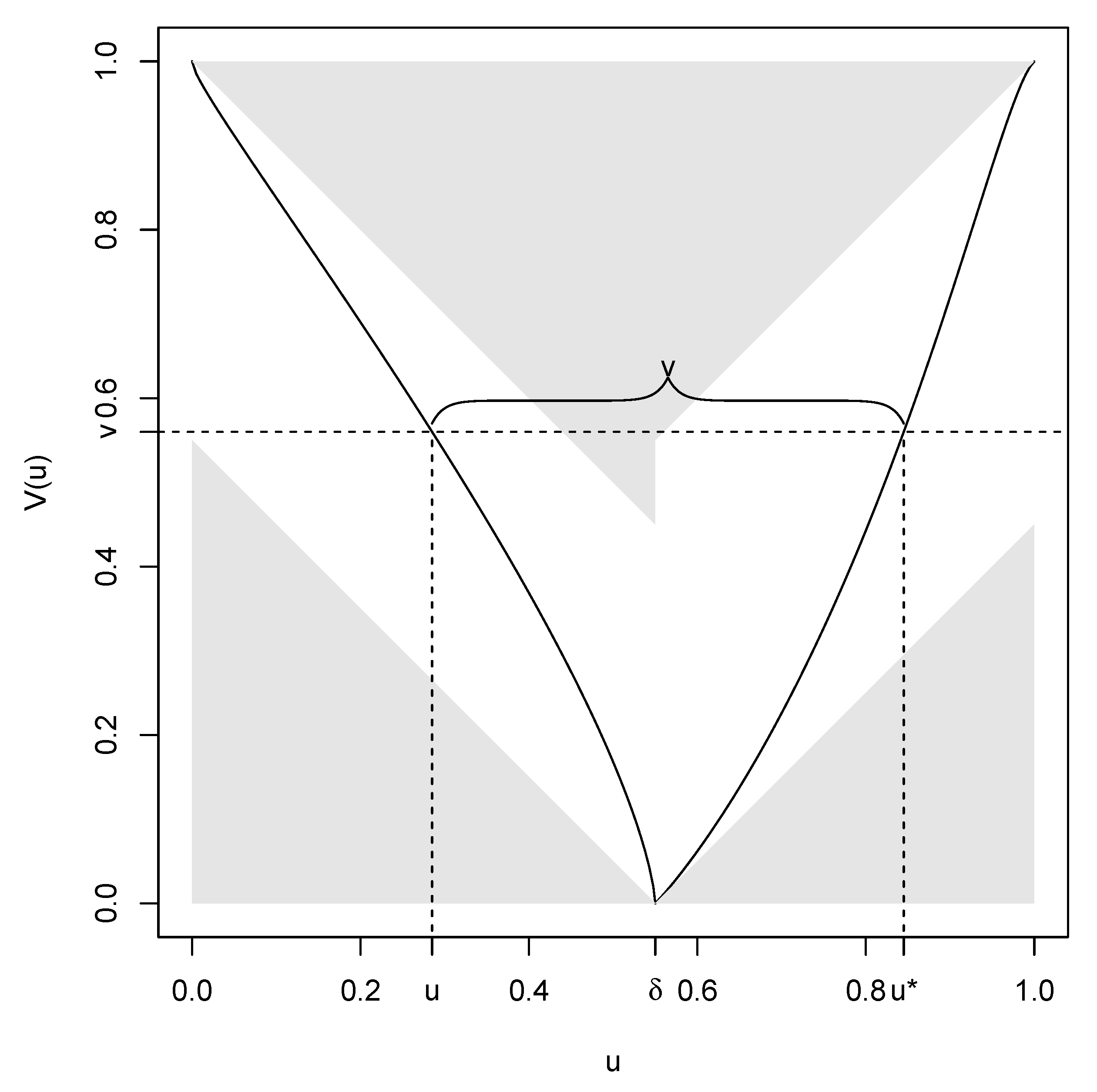
In Figure 3, we show the v-transform ${\mathcal{V}}_{\delta ,\kappa ,\xi }$ when $\delta =0.55$, $\kappa =1.4$ and $\xi =0.65$. We will use this particular v-transform to illustrate further properties of v-transforms and find a characterization.

Figure 3. An asymmetric v-transform from the family defined in (7). For any v-transform, if $v=\mathcal{V}\left(u\right)$ and $u^{*}$ is the dual of u, then the points $(u,0)$, $(u,v)$, $(u^{*},0)$ and $(u^{*},v)$ form the vertices of a square. For the given fulcrum $\delta$, a v-transform can never enter the gray shaded area of the plot.

3.2. Characterizing v-Transforms

It is easily verified that any v-transform obtained from (4) consists of two arms or branches, described by continuous and strictly monotonic functions; the left arm is decreasing and the right arm increasing. See Figure 3 for an illustration. At the fulcrum $\delta$, we have $\mathcal{V}\left(\delta \right)=0$. Every point $u\in [0,1]\backslash \left\{\delta \right\}$ has a dual point $u^{*}$ on the opposite side of the fulcrum such that $\mathcal{V}\left(u^{*}\right)=\mathcal{V}\left(u\right)$. Dual points can be interpreted as the quantile probability levels of the distribution of X that give rise to the same level of volatility.

We collect these properties together in the following lemma and add one further important property that we refer to as the square property of a v-transform; this property places constraints on the shape that v-transforms can take and is illustrated in Figure 3.

Lemma 2.

A v-transform is a mapping $\mathcal{V}:[0,1]\to [0,1]$ with the following properties:

1. 

$\mathcal{V}\left(0\right)=\mathcal{V}\left(1\right)=1$;

2. 

There exists a point δ known as the fulcrum such that $0<\delta <1$ and $\mathcal{V}\left(\delta \right)=0$;

3. 

$\mathcal{V}$ is continuous;

4. 

$\mathcal{V}$ is strictly decreasing on $[0,\delta ]$ and strictly increasing on $[\delta ,1]$;

5. 

Every point $u\in [0,1]\backslash \left\{\delta \right\}$ has a dual point $u^{*}$ on the opposite side of the fulcrum satisfying $\mathcal{V}\left(u\right)=\mathcal{V}\left(u^{*}\right)$ and $|u^{*}-u|=\mathcal{V}\left(u\right)$ (square property).

It is instructive to see why the square property must hold. Consider Figure 3 and fix a point $u\in [0,1]\backslash \left\{\delta \right\}$ with $\mathcal{V}\left(u\right)=v$. Let $U\sim U(0,1)$ and let $V=\mathcal{V}\left(U\right)$. The events $\left\{V\le v\right\}$ and $\left\{min(u,u^{*})\le U\le max(u,u^{*})\right\}$ are the same and hence the uniformity of V under a v-transform implies that

$$v=\mathbb{P}(V\le v)=\mathbb{P}(min(u,u^{*})\le U\le max(u,u^{*}))=|u^{*}-u|.$$

(9)

The properties in Lemma 2 could be taken as the basis of an alternative definition of a v-transform. In view of (9), it is clear that any mapping $\mathcal{V}$ that has these properties is a uniformity-preserving transformation. We can characterize the mappings $\mathcal{V}$ that have these properties as follows.

Theorem 1.

A mapping $\mathcal{V}:[0,1]\to [0,1]$ has the properties listed in Lemma 2 if and only if it takes the form

$$\mathcal{V}\left(u\right)=\left\{\begin{array}{cc}(1-u)-(1-\delta )\Psi \left(\frac{u}{\delta }\right)\hfill & u\le \delta ,\hfill \\ u-\delta {\Psi }^{-1}\left(\frac{1-u}{1-\delta }\right)\hfill & u>\delta ,\hfill \end{array}\right.$$

(10)

where Ψ is a continuous and strictly increasing distribution function on $[0,1]$.

Our arguments so far show that every v-transform must have the form (10). It remains to verify that every uniformity-preserving transformation of the form (10) can be obtained from construction (4), and this is the purpose of the final result of this section. This allows us to view Definition 2, Lemma 2, and the characterization (10) as three equivalent approaches to the definition of v-transforms.

Proposition 3.

Let $\mathcal{V}$ be a uniformity-preserving transformation of the form (10) and $F_X$ a continuous distribution function. Then, $\mathcal{V}$ can be obtained from construction (4) using any volatility proxy transformation with change point ${\mu }_T=F_X^{-1}\left(\delta \right)$ and profile

$$g_T\left(x\right)=F_X^{-1}\left(F_X({\mu }_T-x)+\mathcal{V}\left(F_X({\mu }_T-x)\right)\right)-{\mu }_T,x\ge 0.$$

(11)

Henceforth, we can view (10) as the general equation of a v-transform. Distribution functions $\Psi$ on $[0,1]$ can be thought of as generators of v-transforms. Comparing (10) with (7), we see that our parametric family ${\mathcal{V}}_{\delta ,\kappa ,\xi }$ is generated by $\Psi \left(x\right)=exp(-\kappa (-{(lnx)}^{\xi }))$. This is a 2-parameter distribution whose density can assume many different shapes on the unit interval including increasing, decreasing, unimodal, and bathtub-shaped forms. In this respect, it is quite similar to the beta distribution which would yield an alternative family of v-transforms. The uniform distribution function $\Psi \left(x\right)=x$ gives the family of linear v-transforms ${\mathcal{V}}_{\delta }$.

In applications, we construct models starting from the building blocks of a tractable v-transform $\mathcal{V}$ such as (7) and a distribution $F_X$; from these, we can always infer an implied profile function $g_T$ using (11). The alternative approach of starting from $g_T$ and $F_X$ and constructing $\mathcal{V}$ via (4) is also possible but can lead to v-transforms that are cumbersome and computationally expensive to evaluate if $F_X$ and its inverse do not have simple closed forms.

3.3. V-Transforms and Copulas

If two uniform random variables are linked by the v-transform $V=\mathcal{V}\left(U\right)$, then the joint distribution function of $(U,V)$ is a special kind of copula. In this section, we derive the form of the copula, which facilitates the construction of stochastic processes using v-transforms.

To state the main result, we use the notation ${\mathcal{V}}^{-1}$ and ${\mathcal{V}}^{\prime }$ for the the inverse function and the gradient function of a v-transform $\mathcal{V}$. Although there is no unique inverse ${\mathcal{V}}^{-1}\left(v\right)$ (except when $v=0$), the fact that the two branches of a v-transform mutually determine each other allows us to define ${\mathcal{V}}^{-1}\left(v\right)$ to be the inverse of the left branch of the v-transform given by ${\mathcal{V}}^{-1}:[0,1]\to [0,\delta ],{\mathcal{V}}^{-1}\left(v\right)=inf\{u:\mathcal{V}\left(u\right)=v\}$. The gradient ${\mathcal{V}}^{\prime }\left(u\right)$ is defined for all points $u\in [0,1]\backslash \left\{\delta \right\}$, and we adopt the convention that ${\mathcal{V}}^{\prime }\left(\delta \right)$ is the left derivative as $u\to \delta$.

Theorem 2.

Let V and U be random variables related by the v-transform $V=\mathcal{V}\left(U\right)$.

1. 

The joint distribution function of $(U,V)$ is given by the copula

$$C(u,v)=\left(U\le u,V\le v\right)=\left\{\begin{array}{cc}0\hfill & u<{\mathcal{V}}^{-1}\left(v\right)\hfill \\ u-{\mathcal{V}}^{-1}\left(v\right)\hfill & {\mathcal{V}}^{-1}\left(v\right)\le u<{\mathcal{V}}^{-1}\left(v\right)+v\hfill \\ v\hfill & u\ge {\mathcal{V}}^{-1}\left(v\right)+v.\hfill \end{array}\right.$$

(12)

2. 

Conditional on $V=v$, the distribution of U is given by

$$U=\left\{\begin{array}{cc}{\mathcal{V}}^{-1}\left(v\right)\hfill & \mathit{with}\mathit{probability}\Delta \left(v\right)\mathit{if}v\ne 0\hfill \\ {\mathcal{V}}^{-1}\left(v\right)+v\hfill & \mathit{with}\mathit{probability}1-\Delta \left(v\right)\mathrm{if}v\ne 0\hfill \\ \delta \hfill & \mathit{if}v=0\hfill \end{array}\right.$$

(13)

where

$$\Delta \left(v\right)=-\frac{1}{{\mathcal{V}}^{\prime }\left({\mathcal{V}}^{-1}\left(v\right)\right)}.$$

(14)

3. 

$\mathbb{E}\left(\Delta \left(V\right)\right)=\delta$.

Remark 1.

In the case of the symmetric v-transform $\mathcal{V}\left(u\right)=|1-2u|$, the copula in (12) takes the form $C(u,v)=max(min(u+\frac{v}{2}-\frac{1}{2},v),0)$. We note that this copula is related to a special case of the tent map copula family $C_{\theta }^{\mathcal{T}}$ in Rémillard (2013) by $C(u,v)=u-C_1^{\mathcal{T}}(u,1-v)$.

For the linear v-transform family, the conditional probability $\Delta \left(v\right)$ in (14) satisfies $\Delta \left(v\right)=\delta$. This implies that the value of V contains no information about whether U is likely to be below or above the fulcrum; the probability is always the same regardless of V. In general, this is not the case and the value of V does contain information about whether U is large or small.

Part (2) of Theorem 2 is the key to stochastically inverting a v-transform in the general case. Based on this result, we define the concept of stochastic inversion of a v-transform. We refer to the function $\Delta$ as the conditional down probability of $\mathcal{V}$.

Definition 3

(Stochastic inversion function of a v-transform). Let $\mathcal{V}$ be a v-transform with conditional down probability Δ. The two-place function ${\mathcal{V}}^{-1}:[0,1]\times [0,1]\to [0,1]$ defined by

$${\mathcal{V}}^{-1}(v,w)=\left\{\begin{array}{cc}{\mathcal{V}}^{-1}\left(v\right)\hfill & ifw\le \Delta \left(v\right)\hfill \\ v+{\mathcal{V}}^{-1}\left(v\right)\hfill & ifw>\Delta \left(v\right).\hfill \end{array}\right.$$

(15)

is the stochastic inversion function of $\mathcal{V}$.

The following proposition, which generalizes Lemma 1, allows us to construct general asymmetric processes that generalize the process of Algorithm 1.

Proposition 4.

Let V and W be iid $U(0,1)$ variables and let $\mathcal{V}$ be a v-transform with stochastic inversion function $\mathcal{V}$. If $U={\mathcal{V}}^{-1}(V,W)$, then $\mathcal{V}\left(U\right)=V$ and $U\sim U(0,1)$.

In Section 4, we apply v-transforms and their stochastic inverses to the terms of time series models. To understand the effect this has on the serial dependencies between random variables, we need to consider multivariate componentwise v-transforms of random vectors with uniform marginal distributions and these can also be represented in terms of copulas. We now give a result which forms the basis for the analysis of serial dependence properties. The first part of the result shows the relationship between copula densities under componentwise v-transforms. The second part shows the relationship under the componentwise stochastic inversion of a v-transform; in this case, we assume that the stochastic inversion of each term takes place independently given $\mathit{V}$ so that all serial dependence comes from $\mathit{V}$.

Theorem 3.

Let $\mathcal{V}$ be a v-transform and let $\mathit{U}={(U_1,\dots ,U_d)}^{\prime }$ and $\mathit{V}={(V_1,\dots ,V_d)}^{\prime }$ be vectors of uniform random variables with copula densities $c_{\mathit{U}}$ and $c_{\mathit{V}}$, respectively.

1. 

If $\mathit{V}={(\mathcal{V}\left(U_1\right),\dots ,\mathcal{V}\left(U_d\right))}^{\prime }$, then

$$c_{\mathit{V}}(v_1,\dots ,v_d)=\sum _{j_1=1}^2\cdots \sum _{j_d=1}^2{c}_{\mathit{U}}(u_{1j_1},\dots ,u_{d{j}_d})\prod _{i=1}^d\Delta {\left(v_i\right)}^{I_{\{j_i=1\}}}{\left(1-\Delta \left(v_i\right)\right)}^{I_{\{j_i=2\}}}$$

(16)

where $u_{i1}={\mathcal{V}}^{-1}\left(v_i\right)$ and $u_{i2}={\mathcal{V}}^{-1}\left(v_i\right)+v_i$ for all $i\in \{1,\dots ,d\}$.

2. 

If $\mathit{U}={({\mathcal{V}}^{-1}(V_1,W_1),\dots ,{\mathcal{V}}^{-1}(V_d,W_d))}^{\prime }$ where $W_1,\dots ,W_d$ are iid uniform random variables that are also independent of $V_1,\dots ,V_d$, then

$$c_{\mathit{U}}(u_1,\dots ,u_d)=c_{\mathit{V}}(\mathcal{V}\left(u_1\right),\dots ,\mathcal{V}\left(u_d\right)).$$

(17)

4. VT-ARMA Copula Models

In this section, we study some properties of the class of time series models obtained by the following algorithm, which generalizes Algorithm 1. The models obtained are described as VT-ARMA processes since they are stationary time series constructed using the fundamental building blocks of a v-transform $\mathcal{V}$ and an ARMA process.

We can add any marginal behaviour in the final step, and this allows for an infinitely rich choice. We can, for instance, even impose an infinite-variance or an infinite-mean distribution, such as the Cauchy distribution, and still obtain a strictly stationary process for $\left(X_t\right)$. We make the following definitions.

Definition 4

(VT-ARMA and VT-ARMA copula process). Any stochastic process $\left(X_t\right)$ that can be generated using Algorithm 2 by choosing an underlying ARMA process with mean zero and variance one, a v-transform $\mathcal{V}$, and a continuous distribution function $F_X$ is a VT-ARMA process. The process $\left(U_t\right)$ obtained at the penultimate step of the algorithm is a VT-ARMA copula process.

Algorithm 2:

Generate $\left(Z_t\right)$ as a causal and invertible Gaussian ARMA process of order $(p,q)$ with mean zero and variance one. Form the volatility PIT process $\left(V_t\right)$ where $V_t=\Phi \left(Z_t\right)$ for all t. Generate iid $U(0,1)$ random variables $\left(W_t\right)$. Form the series PIT process $\left(U_t\right)$ by taking the stochastic inverses $U_t={\mathcal{V}}^{-1}(V_t,W_t)$. Form the process $\left(X_t\right)$ by setting $X_t=F_X^{-1}\left(U_t\right)$ for some continuous cdf $F_X$.

Figure 4 gives an example of a simulated process using Algorithm 2 and the v-transform ${\mathcal{V}}_{\delta ,\kappa ,\xi }$ in (7) with $\kappa =0.9$ and MA parameter $\xi =1.1$. The marginal distribution is a heavy-tailed skewed Student distribution of type (6) with degrees-of-freedom $\nu =3$ and skewness $\gamma =0.8$, which gives rise to more large negative returns than large positive returns. The underlying time series model is an ARMA(1,1) model with AR parameter $\alpha =0.95$ and MA parameter $\beta =-0.85$. See the caption of the figure for full details of parameters.

Figure 4. Top left: realization of length $n=500$ of $\left(X_t\right)$ for a process with a marginal skewed Student distribution (parameters: $\nu =3$, $\gamma =0.8$, $\mu =0.3$, $\sigma =1$) a v-transform of the form (7) (parameters: $\delta =0.50$, $\kappa =0.9$, $\xi =1.1$) and an underlying ARMA process ($\alpha =0.95$, $\beta =-0.85$, ${\sigma }_{ϵ}=0.95$). Top right: the underlying ARMA process $\left(Z_t\right)$ in gray with the conditional mean $\left({\mu }_t\right)$ superimposed in black; horizontal lines at ${\mu }_t=0.5$ (a high value) and ${\mu }_t=-0.5$ (a low value). The corresponding conditional densities are shown in the bottom figures with the marginal density as a dashed line.

In the remainder of this section, we concentrate on the properties of VT-ARMA copula processes $\left(U_t\right)$ from which related properties of VT-ARMA processes $\left(X_t\right)$ may be easily inferred.

4.1. Stationary Distribution

The VT-ARMA copula process $\left(U_t\right)$ of Definition 4 is a strictly stationary process since the joint distribution of $(U_{t_1},\dots ,U_{t_k})$ for any set of indices $t_1<\cdots <t_k$ is invariant under time shifts. This property follows easily from the strict stationarity of the underlying ARMA process $\left(Z_t\right)$ according to the following result, which uses Theorem 3.

Proposition 5.

Let $\left(U_t\right)$ follow a VT-ARMA copula process with v-transform $\mathcal{V}$ and an underlying ARMA(p,q) structure with autocorrelation function $\rho \left(k\right)$. The random vector $(U_{t_1},\dots ,U_{t_k})$ for $k\in \mathbb{N}$ has joint density $c_{P(t_1,\dots ,t_k)}^{\mathrm{Ga}}(\mathcal{V}\left(u_1\right),\dots ,\mathcal{V}\left(u_k\right))$, where $c_{P(t_1,\dots ,t_k)}^{\mathrm{Ga}}$ denotes the density of the Gaussian copula $C_{P(t_1,\dots ,t_k)}^{\mathrm{Ga}}$ and $P(t_1,\cdots ,t_k)$ is a correlation matrix with $(i,j)$ element given by $\rho \left(\right|t_j-t_i\left|\right)$.

An expression for the joint density facilitates the calculation of a number of dependence measures for the bivariate marginal distribution of $(U_t,U_{t+k})$. In the bivariate case, the correlation matrix of the underlying Gaussian copula $C_{P(t,t+k)}^{\mathrm{Ga}}$ contains a single off-diagonal value $\rho \left(k\right)$ and we simply write $C_{\rho \left(k\right)}^{\mathrm{Ga}}$. The Pearson correlation of $(U_t,U_{t+k})$ is given by

$$\begin{array}{cc}\hfill \rho (U_t,U_{t+k})& =12{\int }_0^1{\int }_0^1{u}_1{u}_2{c}_{\rho \left(k\right)}^{\mathrm{Ga}}\left(\mathcal{V}\left(u_1\right),\mathcal{V}\left(u_2\right)\right)\mathrm{d}{u}_1\mathrm{d}{u}_2-3.\hfill \end{array}$$

(18)

This value is also the value of the Spearman rank correlation ${\rho }_S(X_t,X_{t+k})$ for a VT-ARMA process $\left(X_t\right)$ with copula process $\left(U_t\right)$ (since the Spearman’s rank correlation of a pair of continuous random variables is the Pearson correlation of their copula). The calculation of (18) typically requires numerical integration. However, in the special case of the linear v-transform ${\mathcal{V}}_{\delta }$ in (8), we can get a simpler expression as shown in the following result.

Proposition 6.

Let $\left(U_t\right)$ be a VT-ARMA copula process satisfying the assumptions of Proposition 5 with linear v-transform ${\mathcal{V}}_{\delta }$. Let $\left(Z_t\right)$ denote the underlying Gaussian ARMA process. Then,

$$\begin{array}{ccc}\hfill \rho (U_t,U_{t+k})& =& {(2\delta -1)}^2{\rho }_S(Z_t,Z_{t+k})=\frac{6{(2\delta -1)}^{2}arcsin\left(\frac{\rho \left(k\right)}{2}\right)}{\pi }.\hfill \end{array}$$

(19)

For the symmetric v-transform ${\mathcal{V}}_{0.5}$, Equation (19) obviously yields a correlation of zero so that, in this case, the VT-ARMA copula process $\left(U_t\right)$ is a white noise with an autocorrelation function that is zero, except at lag zero. However, even a very asymmetric model with $\delta =0.4$ or $\delta =0.6$ gives $\rho (U_t,U_{t+k})=0.04{\rho }_S(Z_t,Z_{t+k})$ so that serial correlations tend to be very weak.

When we add a marginal distribution, the resulting process $\left(X_t\right)$ has a different auto-correlation function to $\left(U_t\right)$, but the same rank autocorrelation function. The symmetric model of Section 2 is a white noise process. General asymmetric processes $\left(X_t\right)$ are not perfect white noise processes but have only very weak serial correlation.

4.2. Conditional Distribution

To derive the conditional distribution of a VT-ARMA copula process, we use the vector notation ${\mathit{U}}_t={(U_1,\dots ,U_t)}^{\prime }$ and ${\mathit{Z}}_t={(Z_1,\dots ,Z_t)}^{\prime }$ to denote the history of processes up to time point t and ${\mathit{u}}_t$ and ${\mathit{z}}_t$ for realizations. These vectors are related by the componentwise transformation ${\mathit{Z}}_t={\Phi }^{-1}\left(\mathcal{V}\left({\mathit{U}}_t\right)\right)$. We assume that all processes have a time index set given by $t\in \{1,2,\dots \}$.

Proposition 7.

For $t>1$, the conditional density $f_{U_t\mid {\mathit{U}}_{t-1}}(u\mid {\mathit{u}}_{t-1})$ is given by

$$f_{U_t\mid {\mathit{U}}_{t-1}}(u\mid {\mathit{u}}_{t-1})=\frac{\varphi \left(\frac{{\Phi }^{-1}\left(\mathcal{V}\left(u\right)\right)-{\mu }_t}{{\sigma }_{ϵ}}\right)}{{\sigma }_{ϵ}\varphi \left({\Phi }^{-1}\left(\mathcal{V}\left(u\right)\right)\right)}$$

(20)

where ${\mu }_t=\mathbb{E}(Z_t\mid {\mathit{Z}}_{t-1}={\Phi }^{-1}\left(\mathcal{V}\left({\mathit{u}}_{t-1}\right)\right))$ and ${\sigma }_{ϵ}$ is the standard deviation of the innovation process for the ARMA model followed by $\left(Z_t\right)$.

When $\left(Z_t\right)$ is iid white noise ${\mu }_t=0$, ${\sigma }_{ϵ}=1$ and (20) reduce to the uniform density $f_{U_t\mid {\mathit{U}}_{t-1}}(u\mid {\mathit{u}}_{t-1})=1$ as expected. In the case of the first-order Markov AR(1) model $Z_t={\alpha }_1{Z}_{t-1}+{ϵ}_t$, the conditional mean of $Z_t$ is ${\mu }_t={\alpha }_1{\Phi }^{-1}\left(\mathcal{V}\left(u_{t-1}\right)\right)$ and ${\sigma }_{ϵ}^2=1-{\alpha }_1^2$. The conditional density (20) can be easily shown to simplify to $f_{U_t\mid U_{t-1}}(u\mid u_{t-1})=c_{{\alpha }_1}^{\mathrm{Ga}}\left(\mathcal{V}\left(u\right),\mathcal{V}\left(u_{t-1}\right)\right)$ where $c_{{\alpha }_1}^{\mathrm{Ga}}\left(\mathcal{V}\left(u_1\right),\mathcal{V}\left(u_2\right)\right)$ denotes the copula density derived in Proposition 5. In this special case, the VT-ARMA model falls within the class of first-order Markov copula models considered by Chen and Fan (2006), although the copula is new.

If we add a marginal distribution $F_X$ to the VT-ARMA copula model to obtain a model for $\left(X_t\right)$ and use similar notational conventions as above, the resulting VT-ARMA model has conditional density

$$f_{X_t\mid {\mathit{X}}_{t-1}}(x\mid {\mathit{x}}_{t-1})=f_X\left(x\right)f_{U_t\mid {\mathit{U}}_{t-1}}(F_X\left(x\right)\mid F_X\left({\mathit{x}}_{t-1}\right))$$

(21)

with $f_{U_t\mid {\mathit{U}}_{t-1}}$ as in (20). An interesting property of the VT-ARMA process is that the conditional density (21) can have a pronounced bimodality for values of ${\mu }_t$ in excess of zero that is in high volatility situations where the conditional mean of $Z_t$ is higher than the marginal mean value of zero; in low volatility situations, the conditional density appears more concentrated around zero. This phenomenon is illustrated in Figure 4. The bimodality in high volatility situations makes sense: in such cases, it is likely that the next return will be large in absolute value and relatively less likely that it will be close to zero.

The conditional distribution function of $\left(X_t\right)$ is $F_{X_t\mid {\mathit{X}}_{t-1}}(x\mid {\mathit{x}}_{t-1})=F_{U_t\mid {\mathit{U}}_{t-1}}(F_X\left(x\right)\mid F_X\left({\mathit{x}}_{t-1}\right))$ and hence the $\psi$-quantile $x_{\psi ,t}$ of $F_{X_t\mid {\mathit{X}}_{t-1}}$ can be obtained by solving

$$\psi =F_{U_t\mid {\mathit{U}}_{t-1}}(F_X\left(x_{\psi ,t}\right)\mid F_X\left({\mathit{x}}_{t-1}\right)).$$

(22)

For $\psi <0.5$, the negative of this value is often referred to as the conditional $(1-\psi )$-VaR (value-at-risk) at time t in financial applications.

5. Statistical Inference

In the copula approach to dependence modelling, the copula is the object of central interest and marginal distributions are often of secondary importance. A number of different approaches to estimation are found in the literature. As before, let $x_1,\dots ,x_n$ represent realizations of variables $X_1,\dots ,X_n$ from the time series process $\left(X_t\right)$.

The semi-parametric approach developed by Genest et al. (1995) is very widely used in copula inference and has been applied by Chen and Fan (2006) to first-order Markov copula models in the time series context. In this approach, the marginal distribution $F_X$ is first estimated non-parametrically using the scaled empirical distribution function $F_n^{\left(X\right)}$ (see definition in Section 1) and the data are transformed onto the $(0,1)$ scale. This has the effect of creating pseudo-copula data $u_t=\mathrm{rank}\left(x_t\right)/(n+1)$ where $\mathrm{rank}\left(x_t\right)$ denotes the rank of $x_t$ within the sample. The copula is fitted to the pseudo-copula data by maximum likelihood (ML).

As an alternative, the inference-functions-for-margins (IFM) approach of Joe (2015) could be applied. This is also a two-step method although in this case a parametric model ${\widehat{F}}_X$ is estimated under an iid assumption in the first step and the copula is fitted to the data $u_t={\widehat{F}}_X\left(x_t\right)$ in the second step.

The approach we adopt for our empirical example is to first use the semi-parametric approach to determine a reasonable copula process, then to estimate marginal parameters under an iid assumption, and finally to estimate all parameters jointly using the parameter estimates from the previous steps as starting values.

We concentrate on the mechanics of deriving maximum likelihood estimates (MLEs). The problem of establishing the asymptotic properties of the MLEs in our setting is a difficult one. It is similar to, but appears to be more technically challenging than, the problem of showing consistency and efficiency of MLEs for a Box-Cox-transformed Gaussian ARMA process, as discussed in Terasaka and Hosoya (2007). We are also working with a componentwise transformed ARMA process, although, in our case, the transformation $\left(X_t\right)\to \left(Z_t\right)$ is via the nonlinear, non-increasing volatility proxy transformation $T^{\left(Z\right)}\left(x\right)$ in (5), which is not differentiable at the change point ${\mu }_T$. We have, however, run extensive simulations which suggests good behaviour of the MLEs in large samples.

5.1. Maximum Likelihood Estimation of the VT-ARMA Copula Process

We first consider the estimation of the VT-ARMA copula process for a sample of data $u_1,\dots ,u_n$. Let ${\mathit{\theta }}^{\left(V\right)}$ and ${\mathit{\theta }}^{\left(A\right)}$ denote the parameters of the v-transform and ARMA model, respectively. It follows from Theorem 3 (part 2) and Proposition 5 that the log-likelihood for the sample $u_1,\dots ,u_n$ is simply the log density of the Gaussian copula under componentwise inverse v-transformation. This is given by

$$\begin{array}{cc}\hfill L({\mathit{\theta }}^{\left(V\right)},{\mathit{\theta }}^{\left(A\right)}\mid u_1,\dots ,u_n)& =L^{*}({\mathit{\theta }}^{\left(A\right)}\mid {\Phi }^{-1}\left({\mathcal{V}}_{{\mathit{\theta }}^{\left(V\right)}}\left(u_1\right)\right),\dots ,{\Phi }^{-1}\left({\mathcal{V}}_{{\mathit{\theta }}^{\left(V\right)}}\left(u_n\right)\right))\hfill \\ \hfill & -\sum _{t=1}^{n}ln\varphi \left({\Phi }^{-1}\left({\mathcal{V}}_{{\mathit{\theta }}^{\left(V\right)}}\left(u_t\right)\right)\right)\hfill \end{array}$$

(23)

where the first term $L^{*}$ is the log-likelihood for an ARMA model with a standard N(0,1) marginal distribution. Both terms in the log-likelihood (23) are relatively straightforward to evaluate.

The evaluation of the ARMA likelihood $L^{*}({\mathit{\theta }}^{\left(A\right)}\mid z_1,\dots ,z_n)$ for parameters ${\mathit{\theta }}^{\left(A\right)}$ and data $z_1,\dots ,z_n$ can be accomplished using the Kalman filter. However, it is important to note that the assumption that the data $z_1,\dots ,z_n$ are standard normal requires a bespoke implementation of the Kalman filter, since standard software always treats the error variance ${\sigma }_{ϵ}^2$ as a free parameter in the ARMA model. In our case, we need to constrain ${\sigma }_{ϵ}^2$ to be a function of the ARMA parameters so that $var\left(Z_t\right)=1$. For example, in the case of an ARMA(1,1) model with AR parameter ${\alpha }_1$ and MA parameter ${\beta }_1$, this means that ${\sigma }_{ϵ}^2={\sigma }_{ϵ}^2({\alpha }_1,{\beta }_1)=(1-{\alpha }_1^2)/(1+2{\alpha }_1{\beta }_1+{\beta }_1^2)$. The constraint on ${\sigma }_{ϵ}^2$ must be incorporated into the state-space representation of the ARMA model.

Model validation tests for the VT-ARMA copula can be based on residuals

$$r_t=z_t-{\widehat{\mu }}_t,z_t={\Phi }^{-1}({\mathcal{V}}_{{\widehat{\mathit{\theta }}}^{\left(V\right)}}\left(u_t\right))$$

(24)

where $z_t$ denotes the implied realization of the normalized volatility proxy variable and where an estimate ${\widehat{\mu }}_t$ of the conditional mean ${\mu }_t=\mathbb{E}(Z_t\mid {\mathit{Z}}_{t-1}={\mathit{z}}_t)$ may be obtained as an output of the Kalman filter. The residuals should behave like an iid sample from a normal distribution.

Using the estimated model, it is also possible to implement a likelihood-ratio (LR) test for the presence of stochastic volatility in the data. Under the null hypothesis that ${\mathit{\theta }}^{\left(A\right)}=\mathbf{0}$, the log-likelihood (23) is identically equal to zero. Thus, the size of the maximized log-likelihood $L({\widehat{\mathit{\theta }}}^{\left(V\right)},{\widehat{\mathit{\theta }}}^{\left(A\right)};u_1,\dots ,u_n)$ provides a measure of the evidence for the presence of stochastic volatility.

5.2. Adding a Marginal Model

If $F_X$ and $f_X$ denote the cdf and density of the marginal model and the parameters are denoted ${\mathit{\theta }}^{\left(M\right)}$, then the full log-likelihood for the data $x_1,\dots ,x_n$ is simply

$$\begin{array}{cc}{L}^{\mathrm{full}}(\mathit{\theta }\mid x_1,\dots ,x_n)\hfill & =\sum _{t=1}^{n}ln{f}_X(x_t;{\mathit{\theta }}^{\left(M\right)})\hfill \\ \hfill & \hfill +L\left({\mathit{\theta }}^{\left(V\right)},{\mathit{\theta }}^{\left(A\right)}\mid F_X(x_1;{\mathit{\theta }}^{\left(M\right)}),\dots ,F_X(x_n;{\mathit{\theta }}^{\left(M\right)})\right)\end{array}$$

(25)

where the first term is the log-likelihood for a sample of iid data from the marginal distribution $F_X$ and the second term is (23).

When a marginal model is added, we can recover the implied form of the volatility proxy transformation using Proposition 3. If $\widehat{\delta }$ is the estimated fulcrum parameter of the v-transform, then the estimated change point is ${\widehat{\mu }}_T=F_X^{-1}(\widehat{\delta };{\widehat{\mathit{\theta }}}^{\left(M\right)})$ and the implied profile function is

$$\begin{array}{ccc}\hfill {\widehat{g}}_T\left(x\right)& =& {\widehat{F}}_X^{-1}\left({\widehat{F}}_X({\widehat{\mu }}_T-x)-{\mathcal{V}}_{{\widehat{\mathit{\theta }}}^{\left(V\right)}}\left({\widehat{F}}_X({\widehat{\mu }}_T-x)\right)\right)-{\widehat{\mu }}_T.\hfill \end{array}$$

(26)

Note that is is possible to force the change point to be zero in a joint estimation of marginal model and copula by imposing the constraint $F_X(0;{\mathit{\theta }}^{\left(M\right)})=\delta$ on the fulcrum and marginal parameters during the optimization. However, in our experience, superior fits are obtained when these parameters are unconstrained.

5.3. Example

We analyse $n=1043$ daily log-returns for the Bitcoin price series for the period 2016–2019; values are multiplied by 100. We first apply the semi-parametric approach of Genest et al. (1995) using the log-likelihood (23) which yields the results in Table 1. Different models are referred to by VT(n)-ARMA(p, q), where $(p,q)$ refers to the ARMA model and n indexes the v-transform: 1 is the linear v-transform ${\mathcal{V}}_{\delta }$ in (8); 3 is the three-parameter transform ${\mathcal{V}}_{\delta ,\kappa ,\xi }$ in (7); 2 is the two-parameter v-transform given by ${\mathcal{V}}_{\delta ,\kappa }:={\mathcal{V}}_{\delta ,\kappa ,1}$. In unreported analyses, we also tried the three-parameter family based on the beta distribution, but this had negligible effect on the results.

Table 1. Analysis of daily Bitcoin return data 2016–2019. Parameter estimates, standard errors (below estimates) and information about the fit: SW denotes Shapiro–Wilks p-value; L is the maximized value of the log-likelihood and AIC is the Akaike information criterion.

Model	${\mathit{\alpha }}_1$	${\mathit{\beta }}_1$	$\mathit{\delta }$	$\mathit{\kappa }$	$\mathit{\xi }$	SW	L	AIC
VT(1)-ARMA(1,0)	0.283		0.460			0.515	37.59	−71.17
	0.026		0.001
VT(1)-ARMA(1,1)	0.962	−0.840	0.416			0.197	92.91	−179.81
	0.012	0.028	0.004
VT(2)-ARMA(1,1)	0.965	−0.847	0.463	0.920		0.385	94.73	−181.45
	0.011	0.026	0.001	0.131
VT(3)-ARMA(1,1)	0.962	−0.839	0.463	0.881	0.995	0.407	94.82	−179.64
	0.012	0.028	0.001	0.123	0.154

The column marked L gives the value of the maximized log-likelihood. All values are large and positive showing strong evidence of stochastic volatility in all cases. The model VT(1)-ARMA(1,0) is a first-order Markov model with linear v-transform. The fit of this model is noticeably poorer than the others suggesting that Markov models are insufficient to capture the persistence of stochastic volatility in the data. The column marked SW contains the p-value for a Shapiro–Wilks test of normality applied to the residuals from the VT-ARMA copula model; the result is non-significant in all cases.

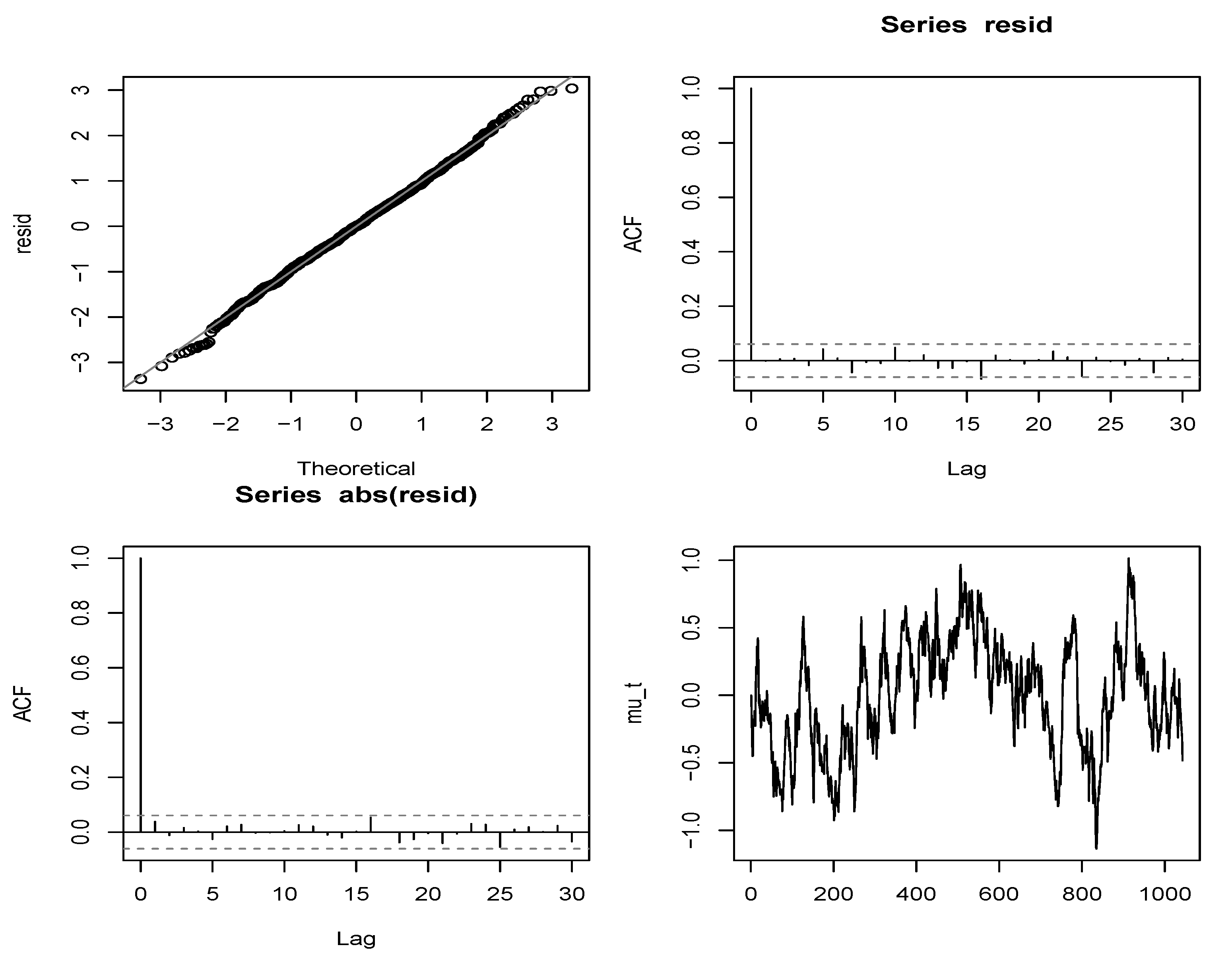
According to the AIC values, the VT(2)-ARMA(1,1) is the best model. We experimented with higher order ARMA processes, but this did not lead to further significant improvements. Figure 5 provides a visual of the fit of this model. The pictures in the panels show the QQplot of the residuals against normal, acf plots of the residuals and squared residuals and the estimated conditional mean process $\left({\widehat{\mu }}_t\right)$, which can be taken as an indicator of high and low volatility periods. The residuals and absolute residuals show very little evidence of serial correlation and the QQplot is relatively linear, suggesting that the ARMA filter has been successful in explaining much of the serial dependence structure of the normalized volatility proxy process.

Figure 5. Plots for a VT(2)-ARMA(1,1) model fitted to the Bitcoin return data: QQplot of the residuals against normal (upper left); acf of the residuals (upper right); acf of the absolute residuals (lower left); estimated conditional mean process $\left({\mu }_t\right)$ (lower right).

We now add various marginal distributions to the VT(2)-ARMA(1,1) copula model and estimate all parameters of the model jointly. We have experimented with a number of location-scale families including Student-t, Laplace (double exponential), and a double-Weibull family which generalizes the Laplace distribution and is constructed by taking back-to-back Weibull distributions. Estimation results are presented for these three distributions in Table 2. All three marginal distributions are symmetric around their location parameters $\mu$, and no improvement is obtained by adding skewness using the construction of Fernández and Steel (1998) described in Section 3.1; in fact, the Bitcoin returns in this time period show a remarkable degree of symmetry. In the table, the shape and scale parameters of the distributions are denoted $\eta$ and $\sigma$, respectively; in the case of Student, an infinite-variance distribution with degree-of-freedom parameter $\eta =1.94$ is fitted, but this model is inferior to the models with Laplace and double-Weibull margins; the latter is the favoured model on the basis of AIC values.

Table 2. VT(2)-ARMA(1,1) model with three different margins: Student-t, Laplace, double Weibull. Parameter estimates, standard errors (alongside estimates) and information about the fit: SW denotes Shapiro–Wilks p-value; L is the maximized value of the log-likelihood and AIC is the Akaike information criterion.

	Student		Laplace		dWeibull
${\alpha }_1$	0.954	0.012	0.953	0.012	0.965	0.021
${\beta }_1$	−0.842	0.026	−0.847	0.025	−0.847	0.035
$\delta$	0.478	0.001	0.480	0.002	0.463	0.000
$\kappa$	0.790	0.118	0.811	0.129	0.939	0.138
$\eta$	1.941	0.005			0.844	0.022
$\mu$	0.319	0.002	0.315	0.002	0.192	0.001
$\sigma$	2.427	0.003	3.194	0.004	2.803	0.214
SW	0.585		0.551		0.376
L	−2801.696		−2791.999		−2779.950
AIC	5617.392		5595.999		5573.899

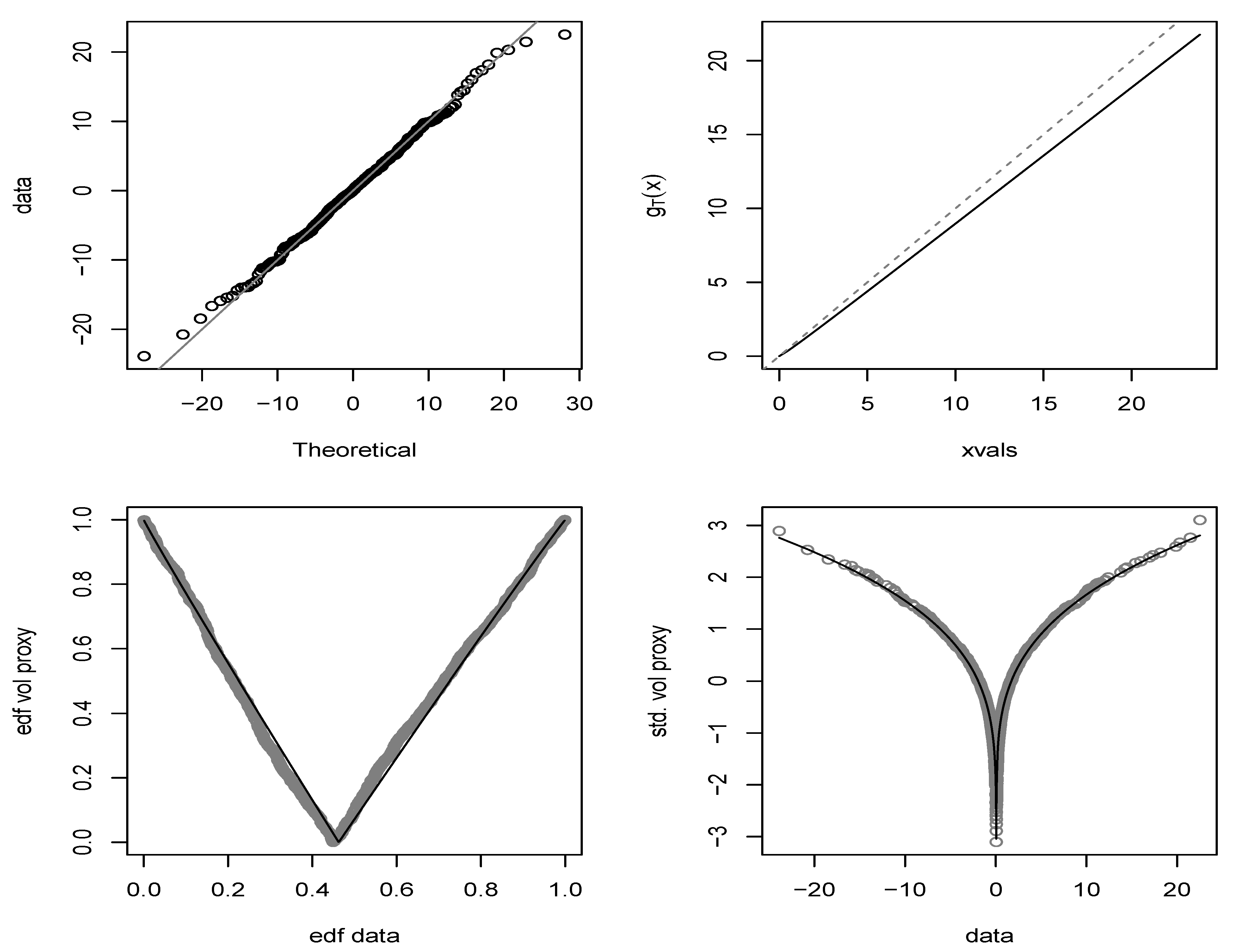
Figure 6 shows some aspects of the joint fit for the fully parametric VT(2)-ARMA(1,1) model with double-Weibull margin. A QQplot of the data against the fitted marginal distribution confirms that the double-Weibull is a good marginal model for these data. Although this distribution is sub-exponential (heavier-tailed than exponential), its tails do not follow a power law and it is in the maximum domain of attraction of the Gumbel distribution (see, for example, McNeil et al. 2015, Chapter 5).

Figure 6. Plots for a VT(2)-ARMA(1,1) model combined with a double Weibull marginal distribution fitted to the Bitcoin return data: QQplot of the data against fitted double Weibull model (upper left); estimated volatility proxy profile function $g_T$ (upper right); estimated v-transform (lower left); implied relationship between data and volatility proxy variable (lower right).

Using (26), the implied volatility proxy profile function ${\widehat{g}}_T$ can be constructed and is found to lie just below the line $y=x$ as shown in the upper-right panel. The change point is estimated to be ${\widehat{\mu }}_T=0.06$. We can also estimate an implied volatility proxy transformation in the equivalence class defined by ${\widehat{g}}_T$ and ${\widehat{\mu }}_T$. We estimate the transformation $T=T^{\left(Z\right)}$ in (5) by taking $\widehat{T}\left(x\right)={\Phi }^{-1}({\mathcal{V}}_{{\widehat{\mathit{\theta }}}^{\left(V\right)}}(F_X(x;{\widehat{\mathit{\theta }}}^{\left(M\right)})))$. In the lower-left panel of Figure 6, we show the empirical v-transform formed from the data $(x_t,\widehat{T}\left(x_t\right))$ together with the fitted parametric v-transform ${\mathcal{V}}_{{\widehat{\mathit{\theta }}}^{\left(V\right)}}$. We recall from Section 1 that the empirical v-transform is the plot $(u_t,v_t)$ where $u_t=F_n^{\left(X\right)}\left(x_t\right)$ and $v_t=F_n^{\left(\widehat{T}\left(X\right)\right)}(\widehat{T}\left(x_t\right))$. The empirical v-transform and the fitted parametric v-transform show a good degree of correspondence. The lower-right panel of Figure 6 shows the volatility proxy transformation $\widehat{T}\left(x\right)$ as a function of x superimposed on the points $(x_t,{\Phi }^{-1}\left(v_t\right))$. Using the curve, we can compare the effects of, for example, a log-return (× 100) of −10 and a log-return of 10. For the fitted model, these are 1.55 and 1.66 showing that the up movement is associated with slightly higher volatility.

As a comparison to the VT-ARMA model, we fit standard GARCH(1,1) models using Student-t and generalized error distributions for the innovations; these are standard choices available in the popular rugarch package in R. The generalized error distribution (GED) contains normal and Laplace as special cases as well as a model that has a similar tail behaviour to Weibull; note, however, that, by the theory of Mikosch and Stărică (2000), the tails of the marginal distribution of the GARCH decay according to a power law in both cases. The results in Table 3 show that the VT(2)-ARMA(1,1) models with Laplace and double-Weibull marginal distributions outperform both GARCH models in terms of AIC values.

Table 3. Comparison of three VT(2)-ARMA(1,1) models with different marginal distributions with two GARCH(1,1) models with different innovation distributions.

	Parameters	AIC
VT-ARMA (Student)	7	5617.39
VT-ARMA (Laplace)	6	5596.00
VT-ARMA (dWeibull)	7	5573.90
GARCH (Student)	5	5629.02
GARCH (GED)	5	5611.53

Figure 7 shows the in-sample 95% conditional value-at-risk (VaR) estimate based on the VT(2)-ARMA(1,1) model which has been calculated using (22). For comparison, a dashed line shows the corresponding estimate for the GARCH(1,1) model with GED innovations.

Figure 7. Plot of estimated 95% value-at-risk (VaR) for Bitcoin return data superimposed on log returns. Solid line shows VaR estimated using the VT(2)-ARMA(1,1) model combined with a double-Weibull marginal distribution; the dashed line shows VaR estimated using a GARCH(1,1) model with GED innovation distribution.

Finally, we carry out an out-of-sample comparison of conditional VaR estimates using the same two models. In this analysis, the models are estimated daily throughout the 2016–2019 period using a 1000-day moving data window and one-step-ahead VaR forecasts are calculated. The VT-ARMA model gives 47 exceptions of the 95% VaR and 11 exceptions of the 99% VaR, compared with expected numbers of 52 and 10 for a 1043 day sample, while the GARCH model leads to 57 and 12 exceptions; both models pass binomial tests for these exception counts. In a follow-up paper (Bladt and McNeil 2020), we conduct more extensive out-of-sample backtests for models using v-transforms and copula processes and show that they rival and often outperform forecast models from the extended GARCH family.

6. Conclusions

This paper has proposed a new approach to volatile financial time series in which v-transforms are used to describe the relationship between quantiles of the return distribution and quantiles of the distribution of a predictable volatility proxy variable. We have characterized v-transforms mathematically and shown that the stochastic inverse of a v-transform may be used to construct stationary models for return series where arbitrary marginal distributions may be coupled with dynamic copula models for the serial dependence in the volatility proxy.

The construction was illustrated using the serial dependence model implied by a Gaussian ARMA process. The resulting class of VT-ARMA processes is able to capture the important features of financial return series including near-zero serial correlation (white noise behaviour) and volatility clustering. Moreover, the models are relatively straightforward to estimate building on the classical maximum-likelihood estimation of an ARMA model using the Kalman filter. This can be accomplished in the stepwise manner that is typical in copula modelling or through joint modelling of the marginal and copula process. The resulting models yield insights into the way that volatility responds to returns of different magnitude and sign and can give estimates of unconditional and conditional quantiles (VaR) for practical risk measurement purposes.

There are many possible uses for VT-ARMA copula processes. Because we have complete control over the marginal distribution, they are very natural candidates for the innovation distribution in other time series models. For example, they could be applied to the innovations of an ARMA model to obtain ARMA models with VT-ARMA errors; this might be particularly appropriate for longer interval returns, such as weekly or monthly returns, where some serial dependence is likely to be present in the raw return data.

Clearly, we could use other copula processes for the volatility PIT process $\left(V_t\right)$. The VT-ARMA copula process has some limitations: the radial symmetry of the underlying Gaussian copula means that the serial dependence between large values of the volatility proxy must mirror the serial dependence between small values; moreover, this copula does not admit tail dependence in either tail and it seems plausible that very large values of the volatility proxy might have a tendency to occur in succession.

To extend the class of models based on v-transforms, we can look for models for the volatility PIT process $\left(V_t\right)$ with higher dimensional marginal distributions given by asymmetric copulas with upper tail dependence. First-order Markov copula models as developed in Chen and Fan (2006) can give asymmetry and tail dependence, but they cannot model the dependencies at longer lags that we find in empirical data. D-vine copula models can model higher-order Markov dependencies and Bladt and McNeil (2020) show that this is a promising alternative specification for the volatility PIT process.

Appendix A.1. Proof of Proposition 1

We observe that, for $x\ge 0$,

$$F_{T\left(X\right)}\left(x\right)=\mathbb{P}({\mu }_T-T_1^{-1}\left(x\right)\le X_t\le {\mu }_T+T_2^{-1}\left(x\right))=F_X({\mu }_T+T_2^{-1}\left(x\right))-F_X({\mu }_T-T_1^{-1}\left(x\right)).$$

$\{X_t\le {\mu }_T\}\iff \{U\le F_X\left({\mu }_T\right)\}$ and in this case

$$\begin{array}{cc}\hfill V=F_{T\left(X\right)}\left(T\left(X_t\right)\right)=F_{T\left(X\right)}\left(T_1({\mu }_T-X_t)\right)& =F_X({\mu }_T+T_2^{-1}\left(T_1({\mu }_T-X_t)\right))-F_X\left(X_t\right)\hfill \\ \hfill & =F_X\left({\mu }_T+g_T\left({\mu }_T-F_X^{-1}\left(U\right)\right)\right)-U.\hfill \end{array}$$

$\{X_t>{\mu }_T\}\iff \{U>F_X\left({\mu }_T\right)\}$ and in this case

$$\begin{array}{cc}\hfill V=F_{T\left(X\right)}\left(T\left(X_t\right)\right)=F_{T\left(X\right)}\left(T_2(X_t-{\mu }_T)\right)& =F_X\left(X_t\right)-F_X({\mu }_T-T_1^{-1}\left(T_2(X_t-{\mu }_T)\right))\hfill \\ \hfill & =U-F_X\left({\mu }_T-g_T^{-1}\left(F_X^{-1}\left(U\right)-{\mu }_T\right)\right).\hfill \end{array}$$

Appendix A.2. Proof of Proposition 2

The cumulative distribution function $F_0\left(x\right)$ of the double exponential distribution is equal to $0.5e^x$ for $x\le 0$ and $1-0.5e^{-x}$ if $x>0$. It is straightforward to verify that

$$F_X(x;\gamma )=\left\{\begin{array}{cc}\delta e^{\gamma x}\hfill & x\le 0\hfill \\ 1-(1-\delta )e^{-\frac{x}{\gamma }}\hfill & x>0\hfill \end{array}\right.\mathrm{and}{F}_X^{-1}(u;\gamma )=\left\{\begin{array}{cc}\frac{1}{\gamma }ln\left(\frac{u}{\delta }\right)\hfill & u\le \delta \hfill \\ -\gamma ln\left(\frac{1-u}{1-\delta }\right)\hfill & u>\delta .\hfill \end{array}\right.$$

When $g_T\left(x\right)=k{x}^{\xi }$, we obtain for $u\le \delta$ that

$$\begin{array}{cc}\hfill {\mathcal{V}}_{\delta ,\kappa ,\xi }\left(u\right)=F_X\left(\frac{k}{{\gamma }^{\xi }}\left(ln{\left(\frac{\delta }{u}\right)}^{\xi }\right);\gamma \right)-u& =1-u-(1-\delta )exp\left(-\frac{k}{{\gamma }^{\xi +1}}{\left(-ln\left(\frac{u}{\delta }\right)\right)}^{\xi }\right).\hfill \end{array}$$

For $u>\delta$, we make a similar calculation.

Appendix A.3. Proof of Theorem 1

It is easy to check that Equation (10) fulfills the list of properties in Lemma 2. We concentrate on showing that a function that has these properties must be of the form (10). It helps to consider the picture of a v-transform in Figure 3. Consider the lines $v=1-u$ and $v=\delta -u$ for $u\in [0,\delta ]$. The areas above the former and below the latter are shaded gray.

The left branch of the v-transform must start at $(0,1)$, end at $(\delta ,0)$, and lie strictly between these lines in $(0,\delta )$. Suppose, on the contrary, that $v=\mathcal{V}\left(u\right)\le \delta -u$ for $u\in (0,\delta )$. This would imply that the dual point $u^{*}$ given by $u^{*}=u+v$ satisfies $u^{*}\le \delta$ which contradicts the requirement that $u^{*}$ must be on the opposite side of the fulcrum. Similarly, if $v=\mathcal{V}\left(u\right)\ge 1-u$ for $u\in (0,\delta )$, then $u^{*}\ge 1$ and this is also not possible; if $u^{*}=1$, then $u=0$, which is a contradiction.

Thus, the curve that links $(0,1)$ and $(\delta ,0)$ must take the form

$$\mathcal{V}\left(u\right)=(\delta -u)\Psi \left(\frac{u}{\delta }\right)+(1-u)\left(1-\Psi \left(\frac{u}{\delta }\right)\right)=(1-u)-(1-\delta )\Psi \left(\frac{u}{\delta }\right)$$

where $\Psi \left(0\right)=0$, $\Psi \left(1\right)=1$ and $0<\Psi \left(x\right)<1$ for $x\in (0,1)$. Clearly, $\Psi$ must be continuous to satisfy the conditions of the v-transform. It must also be strictly increasing. If it were not, then the derivative would satisfy ${\mathcal{V}}^{\prime }\left(u\right)\ge -1$, which is not possible: if at any point $u\in (0,\delta )$, we have ${\mathcal{V}}^{\prime }\left(u\right)=-1$, then the opposite branch of the v-transform would have to jump vertically at the dual point $u^{*}$, contradicting continuity; if ${\mathcal{V}}^{\prime }\left(u\right)>-1$, then $\mathcal{V}$ would have to be a decreasing function at $u^{*}$, which is also a contradiction.

Thus, $\Psi$ fulfills the conditions of a continuous, strictly increasing distribution function on $[0,1]$, and we have established the necessary form for the left branch equation. To find the value of the right branch equation at $u>\delta$, we invoke the square property. Since $\mathcal{V}\left(u\right)=\mathcal{V}\left(u^{*}\right)=\mathcal{V}(u-\mathcal{V}\left(u\right))$, we need to solve the equation $x=\mathcal{V}(u-x)$ for $x\in [0,1]$ using the formula for the left branch equation of $\mathcal{V}$. Thus, we solve $x=1-u+x-(1-\delta )\Psi \left(\frac{u-x}{\delta }\right)$ for x, and this yields the right branch equation as asserted.

Appendix A.4. Proof of Proposition 3

Let $g_T\left(x\right)$ be as given in (11) and let $u\left(x\right)=F_X({\mu }_T-x)$. For $x\in {\mathbb{R}}^{+}$, $u\left(x\right)$ is a continuous, strictly decreasing function of x starting at $u\left(0\right)=\delta$ and decreasing to 0. Since $\Psi$ is a cumulative distribution function, it follows that

$$u^{*}\left(x\right)=u\left(x\right)+\mathcal{V}\left(u\left(x\right)\right)=1-(1-\delta )\Psi \left(\frac{u\left(x\right)}{\delta }\right)$$

is a continuous, strictly increasing function starting at $u^{*}\left(0\right)=\delta$ and increasing to 1. Hence, $g_T\left(x\right)=F_X^{-1}\left(u^{*}\left(x\right)\right)-{\mu }_T$ is continuous and strictly increasing on ${\mathbb{R}}^{+}$ with $g_T\left(0\right)=0$ as required of the profile function of a volatility proxy transformation. It remains to check that, if we insert (11) in (4), we recover $\mathcal{V}\left(u\right)$, which is straightforward.

Appendix A.5. Proof of Theorem 2

• For any $0\le v\le 1$, the event $\{U\le u,V\le v\}$ has zero probability for $u<{\mathcal{V}}^{-1}\left(v\right)$. For $u\ge {\mathcal{V}}^{-1}\left(v\right)$, we have

  $$\{U\le u,V\le v\}=\{{\mathcal{V}}^{-1}\left(v\right)\le U\le min(u,{\mathcal{V}}^{-1}\left(v\right)+v)\}$$

  and hence $\mathbb{P}\left(U\le u,V\le v\right)=min(u,{\mathcal{V}}^{-1}\left(v\right)+v)-{\mathcal{V}}^{-1}\left(v\right)$ and (12) follows.
• We can write $\mathbb{P}\left(U\le u,V\le v\right)=C(u,v)$, where C is the copula given by (12). It follows from the basic properties of a copula that

  $$\mathbb{P}\left(U\le u,V=v\right)=\frac{\mathrm{d}}{\mathrm{d}v}C(u,v)=\left\{\begin{array}{cc}0\hfill & u<{\mathcal{V}}^{-1}\left(v\right)\hfill \\ -\frac{\mathrm{d}}{\mathrm{d}v}{\mathcal{V}}^{-1}\left(v\right)\hfill & {\mathcal{V}}^{-1}\left(v\right)\le u<{\mathcal{V}}^{-1}\left(v\right)+v\hfill \\ 1\hfill & u\ge {\mathcal{V}}^{-1}\left(v\right)+v\hfill \end{array}\right.$$
  This is the distribution function of a binomial distribution, and it must be the case that $\Delta \left(v\right)=-\frac{\mathrm{d}}{\mathrm{d}v}{\mathcal{V}}^{-1}\left(v\right)$. Equation (14) follows by differentiating the inverse.
• Finally, $\mathbb{E}\left(\Delta \left(V\right)\right)=\delta$ is easily verified by making the substitution $x={\mathcal{V}}^{-1}\left(v\right)$ in the integral $\mathbb{E}\left(\Delta \left(V\right)\right)=-{\int }_0^1\frac{1}{{\mathcal{V}}^{\prime }\left({\mathcal{V}}^{-1}\left(v\right)\right)}\mathrm{d}v$.

Appendix A.6. Proof of Proposition 4

It is obviously true that $\mathcal{V}\left({\mathcal{V}}^{-1}(v,W)\right)=v$ for any W. Hence, $\mathcal{V}\left(U\right)=\mathcal{V}\left({\mathcal{V}}^{-1}(V,W)\right)=V$. The uniformity of U follows from the fact that

$$\mathbb{P}\left({\mathcal{V}}^{-1}(V,W)={\mathcal{V}}^{-1}\left(v\right)\mid V=v\right)=\mathbb{P}\left(W\le \Delta \left(v\right)\mid V=v\right)=\mathbb{P}(W\le \Delta \left(v\right))=\Delta \left(v\right).$$

Hence, the pair of random variables $(U,V)$ has the conditional distribution (13) and is distributed according to the copula C in (12).

Appendix A.7. Proof of Theorem 3

• Since the event $\{V_i\le v_i\}$ is equal to the event $\{{\mathcal{V}}^{-1}\left(v_i\right)\le U_i\le {\mathcal{V}}^{-1}\left(v_i\right)+v_i\}$, we first compute the probability of a box $[a_1,b_1]\times \cdots \times [a_d,b_d]$ where $a_i={\mathcal{V}}^{-1}\left(v_i\right)\le {\mathcal{V}}^{-1}\left(v_i\right)+v_i=b_i$. The standard formula for such probabilities implies that the copulas $C_{\mathit{V}}$ and $C_{\mathit{U}}$ are related by

  $$C_{\mathit{V}}(v_1,\dots ,v_d)=\sum _{j_1=1}^2\cdots \sum _{j_d=1}^2{(-1)}^{j_1+\cdots +j_d}{C}_{\mathit{U}}(u_{1j_1},\dots ,u_{d{j}_d});$$

  see, for example, McNeil et al. (2015), p. 221. Thus, the copula densities are related by

  $$c_{\mathit{V}}(v_1,\dots ,v_d)=\sum _{j_1=1}^2\cdots \sum _{j_d=1}^2{c}_{\mathit{U}}(u_{1j_1},\dots ,u_{d{j}_d})\prod _{i=1}^d\frac{\mathrm{d}}{\mathrm{d}{v}_i}{(-1)}^{j_i}{u}_{i{j}_i},$$

  and the result follows if we use (14) to calculate that

  $$\frac{\mathrm{d}}{\mathrm{d}{v}_i}{(-1)}^j{u}_{ij}=\left\{\begin{array}{cc}\frac{\mathrm{d}}{\mathrm{d}{v}_i}\left(-{\mathcal{V}}^{-1}\left(v_i\right)\right)=\Delta \left(v_i\right)\hfill & \mathrm{if}j=1,\hfill \\ \frac{\mathrm{d}}{\mathrm{d}{v}_i}\left(v_i+{\mathcal{V}}^{-1}\left(v_i\right)\right)=1-\Delta \left(v_i\right)\hfill & \mathrm{if}j=2.\hfill \end{array}\right.$$
• For the point $(u_1,\dots ,u_d)\in {[0,1]}^d$, we consider the set of events $A_i\left(u_i\right)$ defined by

  $$A_i\left(u_i\right)=\left\{\begin{array}{cc}\left\{U_i\le u_i\right\}\hfill & \mathrm{if}{u}_i\le \delta \hfill \\ \left\{U_i>u_i\right\}\hfill & \mathrm{if}{u}_i>\delta \hfill \end{array}\right.$$
  The probability $\mathbb{P}(A_1\left(u_1\right),\dots ,A_d\left(u_d\right))$ is the probability of an orthant defined by the point $(u_1,\dots ,u_d)$ and the copula density at this point is given by

  $$c_{\mathit{U}}(u_1,\dots ,u_d)={(-1)}^{{\sum }_{i=1}^d{I}_{\{u_i>\delta \}}}\frac{{\mathrm{d}}^d}{\mathrm{d}{u}_1\cdots \mathrm{d}{u}_d}\mathbb{P}\left(\bigcap _{i=1}^d{A}_i\left(u_i\right)\right).$$
  The event $A_i\left(u_i\right)$ can be written

  $$A_i\left(u_i\right)=\left\{\begin{array}{cc}\left\{V_i\ge \mathcal{V}\left(u_i\right),W_i\le \Delta \left(V_i\right)\right\}\hfill & \mathrm{if}{u}_i\le \delta \hfill \\ \left\{V_i>\mathcal{V}\left(u_i\right),W_i>\Delta \left(V_i\right)\right\}\hfill & \mathrm{if}{u}_i>\delta \hfill \end{array}\right.$$

  and hence we can use Theorem 2 to write

  $$\begin{array}{c}\hfill \mathbb{P}\left(\bigcap _{i=1}^d{A}_i\left(u_i\right)\right)={\int }_{\mathcal{V}\left(u_1\right)}^1\cdots {\int }_{\mathcal{V}\left(u_d\right)}^1{c}_{\mathit{V}}(v_1,\dots ,v_d)\prod _{i=1}^d\Delta {\left(v_i\right)}^{I_{\{u_i\le \delta \}}}{(1-\Delta \left(v_i\right))}^{I_{\{u_i>\delta \}}}\mathrm{d}{v}_1\cdots \mathrm{d}{v}_d.\end{array}$$
  The derivative is given by

  $$\begin{array}{c}\hfill \frac{{\mathrm{d}}^d}{\mathrm{d}{u}_1\cdots \mathrm{d}{u}_d}P\left(\bigcap _{i=1}^d{A}_i\left(u_i\right)\right)={(-1)}^d{c}_{\mathit{V}}(\mathcal{V}\left(u_1\right),\dots ,\mathcal{V}\left(u_d\right))\prod _{i=1}^{d}p{\left(u_i\right)}^{I_{\{u_i\le \delta \}}}{(1-p\left(u_i\right))}^{I_{\{u_i>\delta \}}}{\mathcal{V}}^{\prime }\left(u_i\right)\end{array}$$

  where $p\left(u_i\right)=\Delta \left(\mathcal{V}\left(u_i\right)\right)$ and hence we obtain

  $$c_{\mathit{U}}(u_1,\dots ,u_d)=c_{\mathit{V}}(\mathcal{V}\left(u_1\right),\dots ,\mathcal{V}\left(u_d\right))\prod _{i=1}^d{(-p\left(u_i\right))}^{I_{\{u_i\le \delta \}}}{(1-p\left(u_i\right))}^{I_{\{u_i>\delta \}}}{\mathcal{V}}^{\prime }\left(u_i\right).$$
  It remains to verify that each of the terms in the product is identically equal to 1. For $u_i\le \delta$, this follows easily from (14) since $-p\left(u_i\right)=-\Delta \left(\mathcal{V}\left(u_i\right)\right)=1/{\mathcal{V}}^{\prime }\left(u_i\right)$. For $u_i>\delta$, we need an expression for the derivative of the right branch equation. Since $\mathcal{V}\left(u_i\right)=\mathcal{V}(u_i-\mathcal{V}\left(u_i\right))$, we obtain

  $${\mathcal{V}}^{\prime }\left(u_i\right)={\mathcal{V}}^{\prime }(u_i-\mathcal{V}\left(u_i\right))(1-{\mathcal{V}}^{\prime }\left(u_i\right))={\mathcal{V}}^{\prime }\left(u_i^{*}\right)(1-{\mathcal{V}}^{\prime }\left(u_i\right))⟹{\mathcal{V}}^{\prime }\left(u_i\right)=\frac{{\mathcal{V}}^{\prime }\left(u_i^{*}\right)}{1+{\mathcal{V}}^{\prime }\left(u_i^{*}\right)}$$

  implying that

  $$1-p\left(u_i\right)=1-\Delta \left(\mathcal{V}\left(u_i\right)\right)=1-\Delta \left(\mathcal{V}\left(u_i^{*}\right)\right)=1+\frac{1}{{\mathcal{V}}^{\prime }\left(u_i^{*}\right)}=\frac{1+{\mathcal{V}}^{\prime }\left(u_i^{*}\right)}{{\mathcal{V}}^{\prime }\left(u_i^{*}\right)}=\frac{1}{{\mathcal{V}}^{\prime }\left(u_i\right)}.$$

Appendix A.8. Proof of Proposition 5

Let $V_t=\mathcal{V}\left(U_t\right)$ and $Z_t={\Phi }^{-1}\left(V_t\right)$ as usual. The process $\left(Z_t\right)$ is an ARMA process with acf $\rho \left(k\right)$ and hence $(Z_{t_1},\dots ,Z_{t_k})$ are jointly standard normally distributed with correlation matrix $P(t_1,\dots ,t_k)$. This implies that the joint distribution function of $(V_{t_1},\dots ,V_{t_k})$ is the Gaussian copula with density $c_{P(t_1,\dots ,t_k)}^{\mathrm{Ga}}$ and hence by Part 2 of Theorem 3 the joint distribution function of $(U_{t_1},\dots ,U_{t_k})$ is the copula with density $c_{P(t_1,\dots ,t_k)}^{\mathrm{Ga}}(\mathcal{V}\left(u_1\right),\dots ,\mathcal{V}\left(u_k\right))$.

Appendix A.9. Proof of Proposition 6

We split the integral in (18) into four parts. First, observe that, by making the substitutions $v_1=\mathcal{V}\left(u_1\right)=1-u_1/\delta$ and $v_2=\mathcal{V}\left(u_2\right)=1-u_2/\delta$ on $[0,\delta ]\times [0,\delta ]$, we get

$$\begin{array}{cc}\hfill {\int }_0^{\delta }{\int }_0^{\delta }{u}_1{u}_2{c}_{\rho \left(k\right)}^{\mathrm{Ga}}\left(\mathcal{V}\left(u_1\right),\mathcal{V}\left(u_2\right)\right)\mathrm{d}{u}_1\mathrm{d}{u}_2& ={\delta }^4{\int }_0^1{\int }_0^1(1-v_1)(1-v_2)c_{\rho \left(k\right)}^{\mathrm{Ga}}\left(v_1,v_2\right)\mathrm{d}{v}_1\mathrm{d}{v}_2\hfill \\ \hfill & ={\delta }^4\mathbb{E}\left((1-V_t)(1-V_{t+k})\right)\hfill \\ \hfill & ={\delta }^4\left(1-\mathbb{E}\left(V_t\right)-\mathbb{E}\left(V_{t+k}\right)+\mathbb{E}\left(V_t{V}_{t+k}\right)\right)={\delta }^4\mathbb{E}\left(V_t{V}_{t+k}\right)\hfill \end{array}$$

where $(V_t,V_{t+k})$ has joint distribution given by the Gaussian copula $C_{\rho \left(k\right)}^{\mathrm{Ga}}$. Similarly, by making the substitutions $v_1=\mathcal{V}\left(u_1\right)=1-u_1/\delta$ and $v_2=\mathcal{V}\left(u_2\right)=(u_2-\delta )/(1-\delta )$ on $[0,\delta ]\times [\delta ,1]$, we get

$$\begin{array}{l}{\displaystyle {\int }_0^{\delta }{\int }_{\delta }^1{u}_1{u}_2{c}_{\rho \left(k\right)}^{\mathrm{Ga}}\left(\mathcal{V}\left(u_1\right),\mathcal{V}\left(u_2\right)\right)\mathrm{d}{u}_1\mathrm{d}{u}_2}\hfill \\ ={\int }_0^1{\int }_0^1{\delta }^2(1-\delta )(1-v_1)\left(\delta +(1-\delta )v_2\right)c_{\rho \left(k\right)}^{\mathrm{Ga}}\left(v_1,v_2\right)\mathrm{d}{v}_1\mathrm{d}{v}_2\hfill \\ ={\delta }^3(1-\delta )\mathbb{E}(1-V_t)+{\delta }^2{(1-\delta )}^2\mathbb{E}\left((1-V_t)V_{t+k}\right)=\frac{{\delta }^2(1-\delta )}{2}-{\delta }^2{(1-\delta )}^2\mathbb{E}\left(V_t{V}_{t+k}\right)\hfill \end{array}$$

and the same value is obtained on the quadrant $[\delta ,1]\times [0,\delta ]$. Finally, making the substitutions $v_1=\mathcal{V}\left(u_1\right)=(u_1-\delta )/(1-\delta )$ and $v_2=\mathcal{V}\left(u_2\right)=(u_2-\delta )/(1-\delta )$ on $[\delta ,1]\times [\delta ,1]$, we get

$$\begin{array}{l}{\displaystyle {\int }_{\delta }^1{\int }_{\delta }^1{u}_1{u}_2{c}_{\rho \left(k\right)}^{\mathrm{Ga}}\left(\mathcal{V}\left(u_1\right),\mathcal{V}\left(u_2\right)\right)\mathrm{d}{u}_1\mathrm{d}{u}_2}\\ ={\int }_0^1{\int }_0^1{(1-\delta )}^2\left(\delta +(1-\delta )v_1\right)\left(\delta +(1-\delta )v_2\right)c_{\rho \left(k\right)}^{\mathrm{Ga}}\left(v_1,v_2\right)\mathrm{d}{v}_1\mathrm{d}{v}_2\hfill \\ ={\int }_0^1{\int }_0^1{(1-\delta )}^2\left({\delta }^2+\delta (1-\delta )v_1+\delta (1-\delta )v_2+{(1-\delta )}^2{v}_1{v}_2\right)c_{\rho \left(k\right)}^{\mathrm{Ga}}\left(v_1,v_2\right)\mathrm{d}{v}_1\mathrm{d}{v}_2\hfill \end{array}$$

$$\begin{array}{cc}\hfill & ={\delta }^2{(1-\delta )}^2+\delta {(1-\delta )}^3\mathbb{E}\left(V_t\right)+\delta {(1-\delta )}^3\mathbb{E}\left(V_{t+k}\right)+{(1-\delta )}^4\mathbb{E}\left(V_t{V}_{t+k}\right)\hfill \\ \hfill & =\delta {(1-\delta )}^2+{(1-\delta )}^4\mathbb{E}\left(V_t{V}_{t+k}\right)\hfill \end{array}$$

Collecting all of these terms together yields

$$\begin{array}{cc}\hfill {\int }_0^1{\int }_0^1{u}_1{u}_2{c}_{\rho \left(k\right)}^{\mathrm{Ga}}\left(\mathcal{V}\left(u_1\right),\mathcal{V}\left(u_2\right)\right)\mathrm{d}{u}_1\mathrm{d}{u}_2& =\delta (1-\delta )+{(2\delta -1)}^2\mathbb{E}\left(V_t{V}_{t+k}\right)\hfill \end{array}$$

and, since ${\rho }_S(Z_t,Z_{t+k})=12\mathbb{E}\left(V_t{V}_{t+k}\right)-3$, it follows that

$$\begin{array}{cc}\hfill \rho (U_t,U_{t+k})=12\mathbb{E}\left(U_t{U}_{t+k}\right)-3& =12{\int }_0^1{\int }_0^1{u}_1{u}_2{c}_{\rho \left(k\right)}^{\mathrm{Ga}}\left(\mathcal{V}\left(u_1\right),\mathcal{V}\left(u_2\right)\right)\mathrm{d}{u}_1\mathrm{d}{u}_2-3\hfill \\ \hfill & =12\delta (1-\delta )+12{(2\delta -1)}^2\mathbb{E}\left(V_t{V}_{t+k}\right)-3\hfill \\ & =12\delta (1-\delta )+{(2\delta -1)}^2\left({\rho }_S(Z_t,Z_{t+k})+3\right)-3\hfill \\ \hfill & ={(2\delta -1)}^2{\rho }_S(Z_t,Z_{t+k}).\hfill \end{array}$$

The value of Spearman’s rho ${\rho }_S(Z_t,Z_{t+k})$ for the bivariate Gaussian distribution is well known; see, for example, McNeil et al. (2015).

Appendix A.10. Proof of Proposition 7

The conditional density satisfies

$$\begin{array}{ccc}\hfill f_{U_t\mid {\mathit{U}}_{t-1}}(u\mid {\mathit{u}}_{t-1})& =& \frac{c_{{\mathit{U}}_t}(u_1,\dots ,u_{t-1},u)}{c_{{\mathit{U}}_{t-1}}(u_1,\dots ,u_{t-1})}=\frac{c_{P(1,\dots ,t)}^{\mathrm{Ga}}(\mathcal{V}\left(u_1\right),\dots ,\mathcal{V}\left(u_{t-1}\right),\mathcal{V}\left(u\right))}{c_{P(1,\dots ,t-1)}^{\mathrm{Ga}}(\mathcal{V}\left(u_1\right),\dots ,\mathcal{V}\left(u_{t-1}\right))}.\hfill \end{array}$$

The Gaussian copula density is given in general by

$$c_P^{\mathrm{Ga}}(v_1,\dots ,v_d)=\frac{f_{\mathit{Z}}\left({\Phi }^{-1}\left(v_1\right),\dots ,{\Phi }^{-1}\left(v_d\right)\right)}{{\prod }_{i=1}^d\varphi \left({\Phi }^{-1}\left(v_i\right)\right)}$$

where $\mathit{Z}$ is a multivariate Gaussian vector with standard normal margins and correlation matrix P. Hence, it follows that we can write

$$\begin{array}{ccc}\hfill f_{U_t\mid {\mathit{U}}_{t-1}}(u\mid {\mathit{u}}_{t-1})& =& \frac{f_{{\mathit{Z}}_t}\left({\Phi }^{-1}\left(\mathcal{V}\left(u_1\right)\right),\dots ,{\Phi }^{-1}\left(\mathcal{V}\left(u_{t-1}\right)\right),{\Phi }^{-1}\left(\mathcal{V}\left(u\right)\right)\right)}{f_{{\mathit{Z}}_{t-1}}\left({\Phi }^{-1}\left(\mathcal{V}\left(u_1\right)\right),\dots ,{\Phi }^{-1}\left(\mathcal{V}\left(u_{t-1}\right)\right)\right)\varphi \left({\Phi }^{-1}\left(\mathcal{V}\left(u\right)\right)\right)}\hfill \\ & =& \frac{f_{Z_t\mid {\mathit{Z}}_{t-1}}\left({\Phi }^{-1}\left(\mathcal{V}\left(u\right)\right)\mid {\Phi }^{-1}\left(\mathcal{V}\left({\mathit{u}}_{t-1}\right)\right)\right)}{\varphi \left({\Phi }^{-1}\left(\mathcal{V}\left(u\right)\right)\right)}\hfill \end{array}$$

where $f_{Z_t\mid {\mathit{Z}}_{t-1}}$ is the conditional density of the ARMA process, from which (20) follows easily.