Article

Pricing, Risk and Volatility in Subordinated Market Models

by
Jean-Philippe Aguilar
1,*,
Justin Lars Kirkby
2 and
Jan Korbel
3,4,5,6
1
Covéa Finance, Quantitative Research Team, 8-12 rue Boissy d’Anglas, FR75008 Paris, France
2
School of Industrial and Systems Engineering, Georgia Institute of Technology, Atlanta, GA 30318, USA
3
Section for the Science of Complex Systems, Center for Medical Statistics, Informatics, and Intelligent Systems (CeMSIIS), Medical University of Vienna, Spitalgasse 23, 1090 Vienna, Austria
4
Complexity Science Hub Vienna, Josefstädterstrasse 39, 1080 Vienna, Austria
5
Faculty of Nuclear Sciences and Physical Engineering, Czech Technical University, 11519 Prague, Czech Republic
6
The Czech Academy of Sciences, Institute of Information Theory and Automation, Pod Vodárenskou Věží 4, 182 00 Prague 8, Czech Republic
*
Author to whom correspondence should be addressed.
Risks 2020, 8(4), 124; https://doi.org/10.3390/risks8040124
Submission received: 26 October 2020 / Revised: 11 November 2020 / Accepted: 13 November 2020 / Published: 17 November 2020
(This article belongs to the Special Issue Risks: Feature Papers 2020)

Abstract

:
We consider several market models, where time is subordinated to a stochastic process. These models are based on various time changes in the Lévy processes driving asset returns, or on fractional extensions of the diffusion equation; they were introduced to capture complex phenomena such as volatility clustering or long memory. After recalling recent results on option pricing in subordinated market models, we establish several analytical formulas for market sensitivities and portfolio performance in this class of models, and discuss some useful approximations when options are not far from the money. We also provide some tools for volatility modelling and delta hedging, as well as comparisons with numerical Fourier techniques.

1. Introduction

In this opening section, we provide a general introduction to the class of subordinated market models; we also present the key points investigated in the paper, as well as the work’s overall structure.

1.1. Time Subordination in Financial Modelling

Among the most striking patterns that are observable in financial time series are the phenomena of regime switching, clustering, and long memory or autocorrelation (see e.g., Cont (2007) and references therein). Such stylized facts have been evidenced for several decades, Mandelbrot famously remarking in Mandelbrot (1963) that large price changes tend to cluster together (“large changes tend to be followed by large changes, of either sign, and small changes tend to be followed by small changes”), thus creating periods of market turbulence (high volatility) alternating with periods of relative calm (low volatility). These empirical observations can be described, among other approaches, by agent based models focusing on economic interpretation, such as Lux and Marchesi (2000); Niu and Wang (2013), by tools from statistical mechanics and econophysics (Krawiecki et al. 2002), or by the introduction of multifractals (Calvet and Fischer 2008).
Another prominent approach to describe this subtle volatility behavior consists of introducing a time change in the stochastic process driving the market prices. Besides stochastic volatility, time changed market models also capture several stylized facts, like non-Normality of returns (the presence of jumps, asymmetry) and negative correlation between the returns and their volatility (see a complete overview in Carr and Wu (2004)). They are motivated by the observation that market participants do not operate uniformly through a trading period, but, on the contrary, the volume, and frequency of transactions greatly vary over time. Following the terminology of Geman (2009), the time process is called the stochastic clock, or business time, while the stochastic process for the underlying market (a Brownian motion, or a more general Lévy process) is said to evolve in operational time.
Historically, the first introduction of a time change in a diffusion process goes back to Bochner (1949); it was first applied to financial modeling in Clark (1973) in the context of the cotton futures market and for a continuous-time change. During the late 1990s and early 2000s, the approach was extended to discontinuous time changes, with the introduction of subordinators (i.e., non-negative Lévy processes, see the theoretical details in Bertoin (1999)). In other words, the business time now admits increasing staircase-like realizations, describing peak periods of activity (following, for instance, earning announcements, central bank reports, or major political events) alternating with less busy periods. Perhaps the best-known subordinators are the Gamma process, like in the Variance Gamma (VG) model by Madan et al. (1998), and the inverse Gaussian process, like in the Normal inverse Gaussian (NIG) model by Barndorff-Nielsen (1997). Let us also mention that subordination has been successfully applied in many other fields of applied science. For instance, Gamma subordination has been employed for modeling the deterioration of production equipment in order to optimize their maintenance (see de Jonge et al. (2017) and references therein), and inverse Gaussian subordination was originally introduced in Barndorff-Nielsen (1977) to model the influence of wind on dunes and beach sands.
Recently, a new type of time subordination, based on fractional calculus, has emerged. Indeed, Lévy processes are closely related to fractional calculus because, for many of them (including stable and tempered stable processes), their probability densities satisfy a space fractional diffusion equation (see details and applications to option pricing in Cartea and del-Castillo-Negrete (2007) and in Luchko et al. (2019)). By also allowing the time derivative to be fractional, as, e.g., in Jizba et al. (2018); Kleinert and Korbel (2016); Korbel and Luchko (2016); Tarasov (2019); Tomovski et al. (2020), it provides a new type of subordinated models: while the order of the space fractional derivative controls the heavy tail behavior of the distribution of returns, the order of the time fractional derivative acts as a temporal subordination parameter whose purpose is to capture time-related phenomena, such as temporal risk redistribution. This model, which we shall refer to as the fractional diffusion (FD) model, is an alternative to time-change models, or to subordinated random walks (Gorenflo et al. 2006).
Regarding the practical implementation and valuation of financial derivatives within subordinated market models, the literature is dominated by numerical techniques. In time changed models notably, tools from Fourier transform (Lewis 2001) or Fast Fourier transform (Carr and Madan 1999), and their many refinements, such as the COS method by Fang and Osterlee (2008) or the PROJ method by Kirkby (2015). These methods are popular, notably because such models’ characteristic functions are known in relatively simple closed-forms. Similarly, Cui et al. (2019) provides a numerical pricing framework for a general time changed Markov processes, and Li and Linetsky (2014) employs eigenfunction expansion techniques. However, recently, closed-form pricing formulas have been derived, for the VG model in Aguilar (2020a) and for the NIG model in Aguilar (2020b). The technique has also been employed in the FD model, for vanilla payoffs in Aguilar et al. (2018) and for more exotic options in Aguilar (2020c).
In this paper, we extend these pricing tools to the calculation of risk sensitivities and to profit-and-loss (P&L) explanation, and we provide comparisons between time changed models (such as the NIG and the VG models) and the FD model. Like for the pricing case, risk sensitivities in the context of time changed market models (and of Lévy market models in general) are traditionally evaluated by means of numerical methods based on Fourier inversion (Eberlein et al. 2010; Takahashi and Yamazaki 2008); in the present paper, we will therefore show that they can be expressed in a tractable way, under the form of fast convergent series whose terms explicitly depend on the model parameters. This will allow for us to construct and compare the performance of option based portfolios, and discuss, both quantitatively and qualitatively, the impact on the parameters on risks and P&L. Related topics, such as volatility modeling, will also be discussed.

1.2. Contributions of the Paper

Our purpose in the present work is to investigate and provide details on the following key points:
(a)
demonstrate that the recent pricing formulas for the VG, NIG and FD models are precise and fast converging, and can be successfully used for other applications (e.g., calculations of volatility curve);
(b)
provides efficient closed-form formulas for first and second-order risk sensitivities (Delta, Gamma) and compare them with numerical techniques; and,
(c)
deduce from these formulas several practical features regarding delta-hedging policies and portfolio performance.

1.3. Structure of the Paper

The paper is organized as follows: in Section 2 we recall some fundamental concepts on Lévy processes and option pricing and, in Section 3, we introduce the class of subordinated market models and their main implications in financial modeling.Subsequently, in Section 4, we mention the various closed pricing formulas that have been obtained for this class of models. Approximating these formulas when options are not far from the money, we establish formulas for computing the market volatility in this configuration, thus generalizing the usual Black-Scholes implied volatility. In Section 5 (resp. Section 6), we derive the expressions for the first (resp. second) order market sensitivities, and for the P&L of a delta-hedged portfolio; the impact of the subordination parameter is discussed, and a comparison with numerical techniques is provided. Last, Section 7 is dedicated to concluding remarks.

2. Exponential Lévy Processes

Let us start by recalling some fundamentals on Lévy processes (see full details in Sato (1999) and in Cont and Tankov (2004) for their applications to financial modeling) and, following the classical setup of Schoutens (2003), how they are implemented for the purpose of option pricing.

2.1. Basics of Lévy Processes

Let ( Ω , F , { F t } t 0 , P ) be a probability space that is equipped with its natural filtration. Recall that a Lévy process { X t } t 0 is a stochastically continuous process satisfying X 0 = 0 ( P -almost surely), and whose increments are independent and stationary. This implies that the characteristic function Ψ ( u , t ) : = E P [ e i u X t ] of a Lévy process has a semi-group structure and it admits an infinitesimal generator ψ ( u ) , called Lévy symbol or characteristic exponent, which satisfies
Ψ ( u , t ) = e t ψ ( u ) , ψ ( u ) : = log Ψ ( u , 1 ) .
The characteristic exponent is entirely determined by the triplet ( a , b , Π ( d x ) ) , which corresponds to Lévy–Khintchine representation
ψ ( u ) = a i u 1 2 b 2 u 2 + + e i u x 1 i u x 𝟙 { | x | < 1 } Π ( d x ) ,
where a is the drift and is b the Brownian (or diffusion) component. The measure Π ( d x ) , assumed to be concentrated on R \ { 0 } and satisfy
+ min ( 1 , x 2 ) Π ( d x ) < ,
is called the Lévy measure of the process, and determines its tail behavior and the distribution of jumps. When Π ( R ) < , one speaks of a process with finite activity (or intensity); this is the case for jump-diffusion processes, like in the Kou Model (Kou 2002) or the Merton model (Merton 1976), where only a finite number of jumps can occur on each time interval. When Π ( R ) = , one speaks of a process with infinite activity (or intensity); this class is far richer, because an infinite number of jumps can occur on any finite time interval and, as a consequence, no Brownian component b is even needed to generate a very complex dynamics. A prominent model with infinite activity is the Variance Gamma process, introduced in Madan et al. (1998). When Π ( R ) = 0 (i.e., the process has only positive jumps), one speaks of a subordinator.
An important class of Lévy measures, which will be of particular interest to us in this paper, corresponds to the so-called class of tempered stable processes:
Π ( d x ) : = c + e λ + x x 1 + α + 𝟙 { x > 0 } + c e λ | x | | x | 1 + α 𝟙 { x < 0 } d x .
This class contains several sub-classes, such as the tempered stable subordinators ( c = 0 ) or the stable processes ( λ + = λ = 0 ). When c + = c : = C , α + = α : = Y , λ : = G and λ + : = M , one speaks of a CGMY process (introduced in Carr et al. (2002)). By requiring the further restriction that Y = 0 , we obtain the Variance Gamma process of Madan et al. (1998); the symmetric case G = M was considered earlier in Madan and Seneta (1990). We also note that the CGMY (and VG) models are members of the KoBoL family, see Boyarchenko and Levendorskiĭ (2000).

2.2. Exponential Lévy Motions

Let T > 0 and S : t [ 0 , T ] S t be the market price of some financial asset, seen as the realization of a time dependent random variable { S t } t [ 0 , T ] on the canonical space Ω = R + . We assume that there exists a risk-neutral measure Q under which the instantaneous variations of S t can be written down as:
d S t S t = ( r q ) d t + d X t
where r R is the risk-free interest rate and q 0 is the dividend yield (both being assumed to be deterministic and continuously compounded), and where { X t } t [ 0 , T ] is a Lévy process. Under the dynamics (5), the terminal market price is given by
S T = S t e ( r q + ω ) τ + X τ ,
where τ : = T t is the time horizon and ω is the martingale adjustment (also called convexity adjustment, or compensator), which is determined by the martingale condition
E Q [ S T | F t ] = e ( r q ) τ S t .
Given the form of the exponential process (6), the condition (7) is equivalent to:
ω = ψ ( i ) = log E P e X 1 .

2.3. Option Pricing

Given a path-independent payoff function P , i.e., a positive function depending only on the terminal value S T of the market price and on some strike parameters K 1 , , K N > 0 , then the value at time t of a contingent claim delivering a payoff P at its maturity is equal to the following risk-neutral expectation:
C = E Q e r τ P ( S T , K 1 , , K n ) | F t .
If the Lévy process { X t } t [ 0 , T ] admits a density f ( x , t ) , then the conditional expectation (9) can be achieved by integrating all possible realizations for the payoff over the Lévy density, thus resulting in:
C = e r τ + P ( S t e ( r q + ω ) τ + x , K 1 , , K n ) f ( x , τ ) d x .

3. Subordinated Models

In this section, we introduce the class of subordinated market models, which is, models for which time is driven by a particular subordinator. We also provide a review of their main financial applications.

3.1. Exponential VG Model

3.1.1. Model Characteristics

In the exponential VG model by (Madan et al. 1998), one chooses the Lévy process in (5) to be a VG process; this process is defined by
X t ( V G ) : = θ G t + σ W G t
where W t is the standard Wiener process, and γ ( t , 1 , ν ) is a Gamma process (i.e., a process whose increments γ ( t + h , 1 , ν ) γ ( t , 1 , ν ) follow a Gamma distribution with mean 1 × h and variance ν × h ). It follows from definition (11) that the VG process is actually distributed according to a so-called Normal variance–mean mixture (see Barndorff-Nielsen et al. (1982)), where the mixing distribution is the Gamma distribution; this distribution materializes the business time, and it is a particular case of a tempered stable subordinator, as it admits the following Lévy measure (see Sato (1999) for instance):
Π G ( d x ) = 1 ν e 1 ν x x 𝟙 { x > 0 } d x .
It follows from (12) that Π G ( R ) = , which means that the Gamma process has infinite activity; note also that the Gamma measure (12) is concentrated around 0, which means that most jumps in the business time are small, and become bigger in the high ν regime. The VG process is actually a tempered stable process itself (and, more precisely, a CGMY process), its Lévy measure admitting the following representation:
Π V G ( d x ) = e θ x σ 2 ν | x | e θ 2 σ 2 + 2 ν σ | x | d x .
Note that (13) is symmetric around the origin when θ = 0 (i.e., positive and negative jumps in asset prices occur with the same probability). The density function of the VG process is obtained by integrating the normal density conditionally to the Gamma time-change, and it reads:
f V G ( x , t ) = 2 e θ x σ 2 ν t ν 2 π σ Γ ( t ν ) x 2 2 σ 2 ν + θ 2 t 2 ν 1 4 K t ν 1 2 1 σ 2 2 σ 2 ν + θ 2 | x |
where K a ( X ) denotes the modified Bessel function of the second kind, sometimes also called MacDonald function (see definition and properties in Abramowitz and Stegun (1972)). The Lévy symbol is known in the exact form:
ψ V G ( u ) = 1 ν log 1 i θ ν u + σ 2 ν 2 u 2 ,
allowing for a simple representation for the VG martingale adjustment:
ω V G = ψ V G ( i ) = 1 ν log 1 θ ν σ 2 ν 2 .
Remark 1.
Note that, when θ = 0 and ν , then ω V G σ 2 2 , which is the usual Gaussian adjustment, and, in this limit, the exponential VG model degenerates into the Black–Scholes model (Black and Scholes 1973). The limiting regime, VG ( σ , ν , 0 ) ν 0 BS ( σ ) , is illustrated in Figure 1 for decreasing ν. In particular, ν directly controls the excess kurtosis for the VG model.

3.1.2. Financial Applications

As already noted, the presence of the subordination parameter ν is particularly attractive for modeling time-induced phenomena, as it allows for a non-uniform passage of time. When ν is small, realizations of the Gamma subordinator are quasi-linear, which corresponds to a situation where the business time is the same as the operational time. On the contrary, for bigger values of ν , realizations of the Gamma process are highly discontinuous and staircase-like (because the process is non decreasing), capturing the alternation of intense and quieter trading periods.
The exponential VG model has been successfully tested on real market data and shown to perform better than Black–Scholes or Jump-Diffusion models in multiple situations, e.g., for European-style options on the HSI index in Lam et al. (2002) or for currency options in Madan and Dual (2005). Several extensions of the model have been subsequently developed, such as the generalization of the subordination to a bivariate or multivariate Brownian motion (Luciano and Schoutens 2006; Semeraro 2008) (with an application to basket options calibration in Linders and Stassen (2015)). Other recent extensions include the possibility of negative jumps in the linear drift rate of the price process in Ivanov (2018). Last, let us also mention that the exponential VG model has also found its way to applications in other fields of quantitative finance, such as credit risk in Fiorani et al. (2007).

3.2. Exponential NIG Model

3.2.1. Model Characteristics

In the exponential NIG model (see Barndorff-Nielsen (1997)), one chooses the Lévy process in (5) to be the NIG process, defined by
X t ( N I G ) = β δ 2 I t + δ W I t
where { I t } t [ 0 , T ] follows an Inverse Gamma distribution of shape δ α 2 β 2 and mean rate 1. α > 0 is a tail or steepness parameter controlling the kurtosis of the NIG distribution; the large α regime gives birth to light tails, while small α corresponds to heavier tails. β ( α , α 1 ) is the skewness parameter: β < 0 (resp. β > 0 ) implies that the distribution is skewed to the left (resp. the right), and β = 0 that the distribution is symmetric. δ > 0 is the scale parameter and it plays an analogous role to the variance term σ 2 in the Normal distribution. Let us mention that a location parameter μ R can also be incorporated, but it has no impact on option prices (see e.g., Aguilar (2020b)), and, therefore, we will assume that it is equal to 0. Let us also note that, again, we are in the presence of a tempered stable subordination, as the Lévy measure of the Inverse Gamma process { I t } t [ 0 , T ] satisfies
Π I G ( d x ) = e δ 2 ( α 2 β 2 ) 2 x x 3 2 𝟙 { x > 0 } d x ,
while the Lévy measure of the NIG process itself is given by
Π N I G ( d x ) : = α δ π e β x K 1 ( α | x | ) | x | d x .
It follows from definition (17) that, like in the VG case, the NIG process is also distributed according to a Normal variance-mean mixture, where the mixing distribution is now the IG distribution; this mixture is a particular case of the more general class of hyperbolic processes (see discussion and applications to finance in Eberlein and Keller (1995)), the mixing distributions in that case being the Generalized Inverse Gaussian (GIG) distribution. The probability density function for the NIG process is obtained by an integration of the Normal density over the IG distribution and it reads
f N I G ( x , t ) : = α δ t π e δ t α 2 β 2 + β ( x μ t ) K 1 α ( δ t ) 2 + ( x μ t ) 2 ( δ t ) 2 + ( x μ t ) 2 ,
and its Lévy symbol is given by
ψ N I G ( u ) = δ α 2 ( β + i u ) 2 α 2 β 2 .
It follows that the NIG convexity adjustment reads
ω N I G = ψ N I G ( i ) = δ α 2 ( β + 1 ) 2 α 2 β 2 .
Remark 2.
When α (large steepness regime), then ω N I G σ 2 2 ( 1 + 2 β ) where σ 2 : = δ α ; when, furthermore, β = 0 (symmetric process) then one recovers the usual Gaussian adjustment σ 2 2 and the exponential NIG model degenerates into the Black–Scholes model.

3.2.2. Financial Applications

The exponential NIG model has been proved to provide a distinguished fitting to financial data many times. Let us mention, among others, initial tests for daily returns on Danish and German markets in Rydberg (1997) and, subsequently, on the FTSE All-share index (also known as “Actuaries index”) in Venter and de Jongh (2002). More recently, the impact of high-frequency trading has also been taken into account, and calibrations have been performed on intraday returns, e.g., in Figueroa-López et al. (2012) for different sampling frequencies. Like in the VG case, multivariate extensions have also been considered (see Luciano and Semeraro (2010) and references therein), and applications to credit risk have also been provided (Luciano 2009).
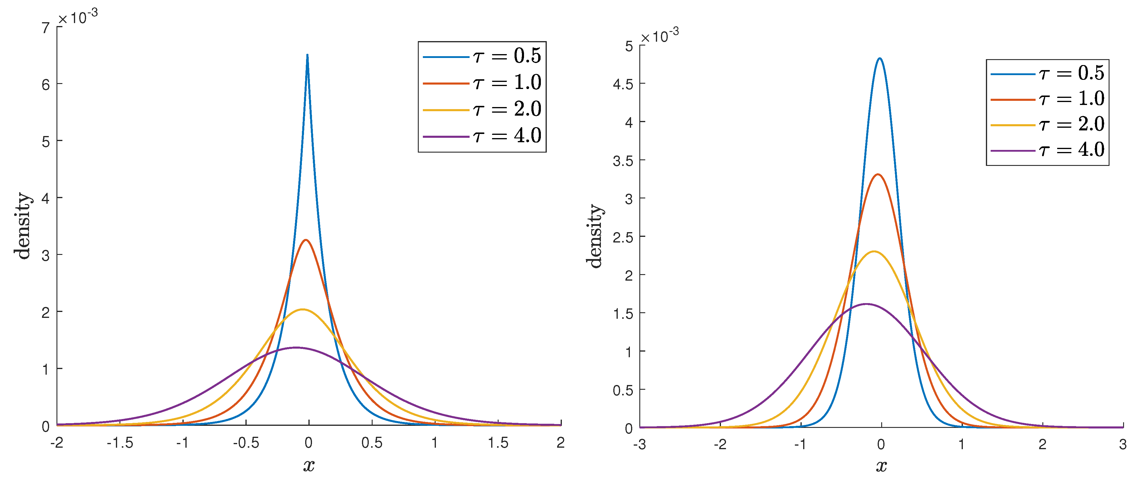
In Figure 2, we display the log-return density for a VG and NIG example, each being recovered from their characteristic functions while using the method of Kirkby (2015). While both models exhibit heavy-tails, the VG model is characterized by a pronounced cusp, especially for shorter maturities. This near singular behavior presents challenges for Fourier pricing methods, and techniques, such as spectral filtering, have been proposed as a remedy Cui et al. (2017); Phelan et al. (2019); Ruijter et al. (2015). In contrast, the closed form pricing formulas presented here exhibit smooth exponential convergence without special handling, as demonstrated in Section 4.

3.3. Fractional Diffusion Model

The FD model by Kleinert and Korbel (2016); Korbel and Luchko (2016) aims at generalizing the Lévy stable model by introducing a time-fractional derivative in the equation governing the probability densities, whose order will be interpreted as a subordination parameter. Before introducing the model and its characteristics, we briefly recall some basics of stable distributions and their link with fractional calculus.

3.3.1. Lévy-Stable Processes and Fractional Derivatives

Taking λ + = λ = 0 and α + = α : = α ( 0 , 2 ) in (4) yields the Lévy measure of the stable (or α -stable) process { X t ( s t a b l e ) } t [ 0 , T ] :
Π s t a b l e ( x ) = c | x | 1 + α 𝟙 { x < 0 } + c + x 1 + α 𝟙 { x > 0 } .
It is known that, when using Feller’s parametrization,
σ α : = ( c + + c ) Γ ( α ) cos π α 2 β : = c + c c + + c
then the Lévy symbol of the stable process can be written as
ψ s t a b l e ( u ) = σ α | u | α 1 i β tan α π 2 sgn u + i a u
where the drift term a equals the expectation E Q [ X t ( s t a b l e ) ] as soon as α ( 1 , 2 ) , that is, for the class of stable Paretian distributions. This class is the one with the greatest financial meaning and historical importance, with initial calibrations going back to Mandelbrot (1963) with α 1.7 for cotton prices; see a comprehensive overview of these distributions in Zolotarev (1986), and of their financial applications in Mittnik and Rachev (2000). However, we may note that, due to the polynomial decay of (23) on the positive axis, the moment generating function and moments of all order do not exist unless c + = 0 , or, equivalently, in terms of the parametrization (24), β = 1 . This condition, which is known as the maximal negative asymmetry (or skewness) hypothesis, is the key assumption in the Finite Moment Log Stable (FMLS) model by Carr and Wu (2003); it follows from (25) that the FMLS martingale adjustment is
ω F M L S = σ 2 α cos π α 2 = 1 π Γ 1 α 2 Γ 1 + α 2 σ 2 α
where we have introduced the 2 normalization, so as to recover the Gaussian adjustment when α = 2 , and where the second equality is a consequence of the reflection formula for the Gamma function; in the limiting case α = 2 , the stable distribution degenerates into the Normal one, and, therefore, the FMLS model recovers the Black–Scholes model.
Another consequence of the characteristic exponent (25) with β = 1 is that the FMLS probability density f F M L S ( x , t ) satisfies the space fractional diffusion equation
f F M L S t + ω α D x α f F M L S ( x , t ) = 0 , x R , t [ 0 , T ] ,
where D x α : = α 2 D x α is a particular case of the Riesz–Feller derivative defined (via its Fourier transform) by
θ D x α f ^ ( u ) = | k | α e i ( sign u ) θ π / 2 f ^ ( u ) , | θ | min { α , α 2 } .
Remark 3.
When θ = 0 , the Riesz–Feller derivative is simply called Riesz derivative (as the operator inverse to the Riesz potential, see all details and definitions e.g., in the classical monograph Samko et al. (1993)); the choice θ = α 2 in Equation (27) is the fractional calculus analogue to the maximal negative asymmetry hypothesis β = 1 . When α = 2 then the Riesz-Feller derivative degenerates into the usual second derivative; in that case, (27) becomes the usual heat equation, whose fundamental solution (the heat kernel) is the probability density of the Wiener process.

3.3.2. Model Characteristics

The FD model generalizes the FMLS model, by allowing the time derivative in the Equation (27) for the probability density to be fractional as well:
* D t γ + ω F D D x α f F D ( x , t ) = 0 , x R , t [ 0 , T ] ,
where α ( 1 , 2 ] , γ ( 0 , α ] and * D γ t denotes the Caputo fractional derivative (see the definitions and properties in Li et al. (2011) for instance); when γ = 1 , it coincides with the usual first-order derivative.
The fundamental solution to (29) has been determined in Mainardi et al. (2001) and admits the following Mellin–Barnes representation
f F D ( x , t ) = 1 α x c i c + i G + * ( s ) 𝟙 { x > 0 } + G * ( s ) 𝟙 { x < 0 } | x | ( μ α , γ t γ ) 1 α s d s 2 i π ,
where we have defined
G + * ( s ) : = Γ ( 1 s ) Γ ( 1 γ s α ) , G * ( s ) : = Γ s α Γ 1 s α Γ ( 1 s ) Γ 1 γ α s Γ α 1 α s Γ 1 α 1 α s .
By analogy with (10), the price of a contingent claim C delivering a path independent payoff P at its maturity is defined to be
C = e r τ + P ( S t e ( r q + ω F D ) τ + x , K 1 , , K n ) f F D ( x , τ ) d x
and the martingale adjustment is defined in terms of the cumulant generating function by
ω F D = log + e x f F D ( x , 1 ) d x .
It has been shown in Aguilar et al. (2018) that ω F D can be conveniently expressed in the form of a series
ω F D = log n = 0 ( 1 ) n n ! Γ ( 1 + α n ) Γ ( 1 + γ α n ) ω F M L S n
where ω F M L S is the FMLS martingale adjustment that is defined in (26), and under the condition that γ ( 1 1 α , α ) ; using a first-order Taylor expansion for log ( 1 + u ) and the expression (26), we obtain the useful approximation:
ω F D = 1 π Γ ( 1 + α ) Γ 1 α 2 Γ 1 + α 2 Γ ( 1 + γ α ) σ 2 α + O σ 2 α .
Remark 4.
When α = 2 , we are left with
ω F D = σ 2 Γ ( 1 + 2 γ ) + O σ 4
which coincides with the Black–Scholes adjustment σ 2 2 when γ = 1 ; we call the situation α = 2 and γ ( 0 , 2 ] the “subordinated Black-Scholes” (sub-BS) model. This is a slight abuse of terminology, because we are not directly in the presence of a subordinating process (i.e., a non decreasing Lévy process) like in the VG and the NIG cases; subordination is achieved here via the introduction of a fractional time derivative whose order γ acts as a supplementary degree of freedom in the time dynamics. When γ = 1 , then the sub-BS model recovers the Black–Scholes model, like the VG model with ν 0 and the NIG model with α ; we summarize the situation in Table 1.

3.3.3. Financial Applications

The purpose of the FD model is to allow more flexibility in the risk redistribution of returns. When the tail index α departs from 2, the model shifts the returns towards more significant losses due to the presence of the left fat tail. Similarly, when the order of the fractional derivative γ is different from 1, the risk is shifted either towards shorter ( γ < 1 ) or longer ( γ > 1 ) maturities: for instance, when γ < 1 , the prices of short term options increase while the prices of long term options slightly decrease (see details, e.g., in Korbel and Luchko (2016)). This behavior is particularly relevant in periods of stressed market conditions: for instance, it has been observed during the 2020 market turmoils (consecutive to the COVID19 pandemics) that short-term implied volatility on the Euro Stoxx 50 index had increased sharply while remaining more stable for long-term options. Several calibrations have been made, notably on market data from turbulent times; in particular, in Kleinert and Korbel (2016), the FD model has been calibrated on data from S&P 500 options traded during November 2008. Such calibrations have shown that α could be quite different from 2: typically, α 1.6–1.7, that turns out to be quite remote from the log-normal hypothesis ( α = 2 ), but relatively close to the initial Mandelbrot estimate for the stable law on cotton futures market (Mandelbrot 1963). Moreover, it has been noted that both fractional parameters α and γ appeared to vary simultaneously and in the same direction, leaving the diffusion scaling exponent γ / α relatively stable.

4. Pricing and Volatility Modelling

In this section, we first recall the pricing formulas that were obtained in recent works for the VG, NIG, and FD models, in the case of a European option C delivering a payoff equal to [ S T K ] + at maturity. Then, we discuss some volatility properties when asset prices are not far from the money. In all of the following, we will denote the forward strike price and the log-forward moneyness by
F : = K e r τ , k : = log S t K + ( r q ) τ .
We will also use the notations
k V G : = k + ω V G τ , k N I G : = k + ω N I G τ , k F D : = k + ω F D τ
and, in the specific case of the VG model, we will denote
τ ν : = τ ν 1 2 σ ν : = σ ν 2 .
We will assume that the underlying VG (resp. NIG) processes are symmetric, which is, θ = 0 (resp. β = 0 ); this is to simplify the notations, but also because symmetric time-changed models extend the Black–Scholes setup (see Table 1). Therefore, we will be better able to compare the results with usual formulas known in the Black-Scholes model. We will also assume that τ ν Q ; note that this condition is not restrictive, due to the density of Q in R : if τ ν Q , it is easy to make τ ν irrational by adding an arbitrary small perturbation, for instance, τ ν τ ν + e / 10 10 ). Last, whenever the exponential NIG model is concerned, we will always assume that
| k N I G | δ τ < 1
to ensure the convergence of the series. Please note that this condition is automatically satisfied when options are not far from the money because, in this case, k N I G is small. When S t is far from K, condition (40) necessitates a restriction on options maturities in order to be satisfied; for a typical set of parameters, maturities shorter than two or three months should be excluded, which remains a reasonable limitation (see details in Aguilar (2020b)).
For convenience, we summarize the pricing formulas for a European call option.
Formula 1
(European call: pricing formulas).
(i) The value at time t of a European call option in the exponential VG model is:
-
(OTM price) If k V G < 0 ,
C V G ( k V G , σ ν ) = F 2 Γ ( τ ν ) n 1 = 0 n 2 = 1 ( 1 ) n 1 n 1 ! Γ ( n 1 + n 2 + 1 2 + τ ν ) Γ ( n 1 + n 2 2 + 1 ) k V G σ ν n 1 σ ν n 2 + 2 Γ ( 2 n 1 n 2 1 2 τ ν ) Γ ( n 1 + 1 2 τ ν ) k V G σ ν 2 n 1 + 1 + 2 τ ν ( k V G ) n 2 .
-
(ITM price) If k V G > 0 ,
C V G + ( k V G , σ ν ) = S t e q τ F C V G ( k V G , σ ν ) .
-
(ATM price) If k V G = 0 ,
C V G ( k V G , σ ν ) = C V G + ( k V G , σ ν ) = F 2 Γ ( τ ν ) n = 1 Γ ( n + 1 2 + τ ν ) Γ ( n 2 + 1 ) σ ν n .
(ii) The value at time t of a European call option in the exponential NIG model is:
C N I G = F α e α δ τ π n 1 = 0 n 2 = 1 k N I G n 1 n 1 ! Γ ( 1 + n 1 + n 2 2 ) K n 1 n 2 + 1 2 ( α δ τ ) δ τ 2 α n 1 + n 2 + 1 2 .
(iii) The value at time t of a European call option in the FD model is:
C F D = F α n 1 = 0 n 2 = 1 k F D n 1 n 1 ! Γ ( 1 + γ n 1 + n 2 α ) ( ω F D τ γ ) n 1 + n 2 α .
Proof. 
(i) is proved in Aguilar (2020a), (ii) is proved in Aguilar (2020b) and (iii) in Aguilar et al. (2018). □
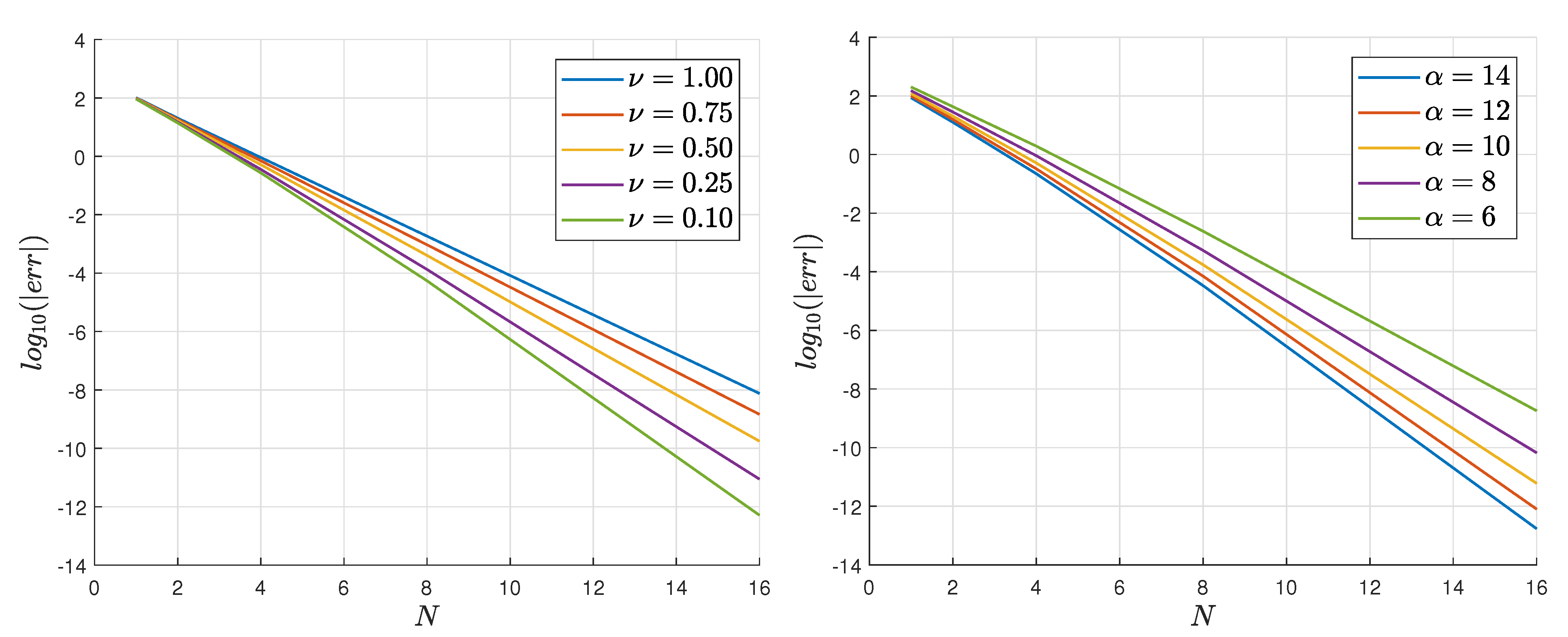
The pricing formulas in Formula (1) converge exponentially fast to the true prices, as exhibited in Figure 3 for the VG model (Left). The reference prices are obtained with N = 50 terms, and they are verified by the method of Kirkby (2015). Recalling Remark 1, VG ( σ , ν , 0 ) ν 0 BS ( σ ) , and fewer terms are required to accurately price the option as ν 0 . A nearly identical convergence profile is observed for NIG (Right), displayed for several values of α . Recalling that NIG ( α , 0 , δ ) α BS ( δ / α ) (see Table 1), we again see that fewer terms are required in order to accurately price under NIG for larger α .

4.1. At-the-Money Forward Approximations

Let us assume that options are at-the-money forward (ATMF), that is, S t = F (or, equivalently, k = 0 ). If we approximate the European call price in the exponential VG model by the first term of the series (41), which is, the term for n 1 = 0 , n 2 = 1 , we obtain (recall that Γ ( 3 / 2 ) = π / 2 ):
C V G = S t 2 π Γ ( 1 2 + τ ν ) Γ ( τ ν ) σ ν .
Using the Stirling approximation for the Gamma function, we know that
Γ 1 2 + τ ν Γ τ ν ν 0 τ ν ,
and, therefore, in the low variance regime, we recover the well-known approximation for the ATMF Black–Scholes price
C B S S t 2 π σ τ .
The approximation (48) is often known to market practitioners under the form C 0.4 S σ τ , because 1 / 2 π = 0.399 , and it was first derived in Brenner and Subrahmanyam (1994).
In a similar way, the ATMF price in the exponential NIG model can be approximated by the first term of the series (44), resulting in
C N I G = S t δ τ e α δ τ π K 0 ( α δ τ ) .
Using the large argument behavior of the Bessel function (see Abramowitz and Stegun (1972))
K 0 ( α δ τ ) α π 2 α δ τ e α δ τ ,
it is immediate to see that (49) also recovers the approximation (48) in the large steepness regime, with σ 2 : = δ / α . Likewise, in the FD model, the ATMF price is approximated by the first term of the series (45), resulting in
C F D = S t α 1 Γ ( 1 + γ α ) ( ω F D τ γ ) 1 α .
Taking α = 2 and using (36), the ATMF price in the sub-BS model becomes
C s u b B S = S t 2 1 Γ ( 1 + γ 2 ) Γ ( 1 + 2 γ ) σ τ γ 2
which recovers (48) when γ 1 .

4.2. Implied Volatility

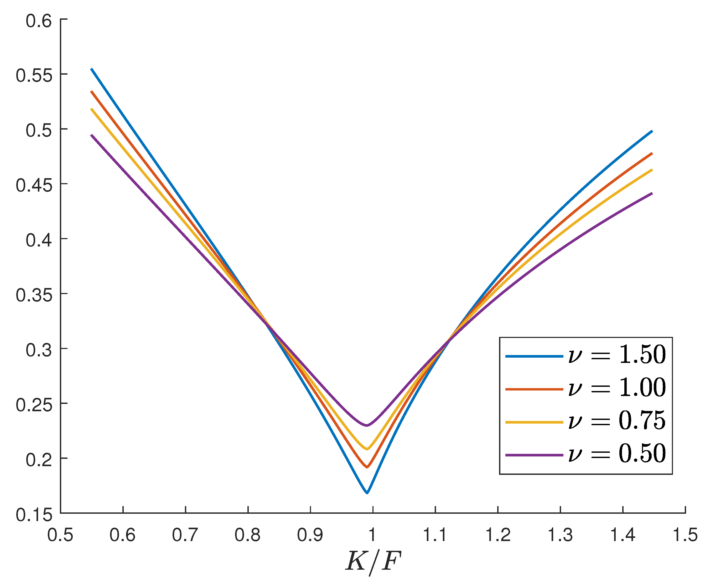
One key benefit of the subordinated models is their ability to capture the heavy-tails that were observed in financial markets. For the VG model, ν directly controls the tail-heaviness, as illustrated in Figure 4. In particular, large values of ν lead to steep implied volatility smiles. The ATMF prices that are obtained in Section 4.1 are helpful to approximate the implied volatility σ I of the subordinated models, when S t is close to F. Denoting by C t the market price of an ATMF European call option at time t and inverting (46), we immediately see that the VG implied volatility is
σ V G = 2 π ν Γ ( τ ν ) Γ ( 1 2 + τ ν ) C t S t ,
and, similarly, inverting Equation (52), the sub-BS implied volatility is
σ s u b B S = 2 Γ ( 1 + 2 γ ) Γ ( 1 + γ 2 ) τ γ 2 C t S t .
As expected, VG and sub-BS both implied volatilities recover the BS implied volatility in their limiting regimes ( ν 0 and γ 1 ):
σ B S = 2 π τ C t S t .
In the NIG case, things are a bit more complicated, because one has to solve
S t δ τ e α δ τ π K 0 ( α δ τ ) = C t
for which there is no exact solution in an analytical form. Nevertheless, an analytical approximation can be determined by using Hankel’s expression for the Bessel function (see Andrews (1992) or any monograph on special functions), which goes, as follows: define, for ρ R ,
a 0 ( ρ ) = 1 a k ( ρ ) = ( 4 ρ 2 1 2 ) ( 4 ρ 2 3 2 ) ( 4 ρ 2 ( 2 k 1 ) 2 ) k ! 8 k , k 1 ,
then, for large z and fixed ρ , we have:
K ρ ( z ) = z π 2 z e z k = 0 a k ( ρ ) z k .
In particular, when 4 ρ 2 1 = 0 , i.e., when ρ = 1 2 , all the a k ( ρ ) are null in definition (57) when k 1 , and we are left with:
K 1 2 ( z ) = π 2 z e z
for all z. Using (58) up to k = 1 for z = α δ τ and inserting into (56), we are left with the quadratic equation
X 2 α 2 π C t S t X 1 8 = 0 ( X : = α δ τ ) ,
whose positive solution reads
X = 1 2 α 2 π C t S t + 2 π α 2 C t 2 S t 2 + 1 2 .
Taylor expanding for large α and turning back to the δ variable, we obtain
δ = 2 π α τ C t 2 S t 2 + 1 4 α τ + O 1 α 3
which, at first order, recovers (55) for σ 2 : = δ / α . We summarize these results in Table 2.

5. First-Order Sensitivities

The sensitivity of a contingent claim C to the underlying asset, often denoted Delta or Δ , is defined by Δ : = C / S t ; by deriving Formula (1) with respect to S t and re-arranging the terms, we obtain the following expressions for European options in subordinated market models:
Formula 2
(European call: Delta).
(i) The Delta at time t of a European call option in the exponential VG model is:
-
(OTM sensitivity) If k V G < 0 ,
Δ V G ( k V G , σ ν ) = F 2 S t Γ ( τ ν ) n 1 = 0 n 2 = 1 ( 1 ) n 1 n 1 ! n 1 Γ ( n 1 + n 2 + 1 2 + τ ν ) Γ ( n 1 + n 2 2 + 1 ) k V G σ ν n 1 1 σ ν n 2 1 + 2 Γ ( 2 n 1 n 2 2 τ ν ) Γ ( n 1 + 1 2 τ ν ) k V G σ ν 2 n 1 + 1 + 2 τ ν ( k V G ) n 2 1 .
-
(ITM sensitivity) If k V G > 0 ,
Δ V G + ( k V G , σ ν ) = e q τ Δ V G ( k V G , σ ν ) .
-
(ATM sensitivity) If k V G = 0 ,
Δ V G ( k V G , σ ν ) = Δ V G + ( k V G , σ ν ) = F 2 S t Γ ( τ ν ) n = 1 Γ ( n 2 + τ ν ) Γ ( n + 1 2 ) σ ν n 1 .
(ii) The Delta at time t of a European call option in the exponential NIG model is:
Δ N I G = F α e α δ τ S t π n 1 = 0 n 2 = 1 k N I G n 1 n 1 ! Γ ( n 1 + n 2 + 1 2 ) K n 1 n 2 2 + 1 ( α δ τ ) δ τ 2 α n 1 + n 2 2 .
(iii) The Delta at time t of a European call option in the FD model is:
Δ F D = F α S t n 1 = 0 n 2 = 0 k F D n 1 n 1 ! Γ ( 1 + γ n 1 + n 2 α ) ( ω F D τ γ ) n 1 + n 2 α .
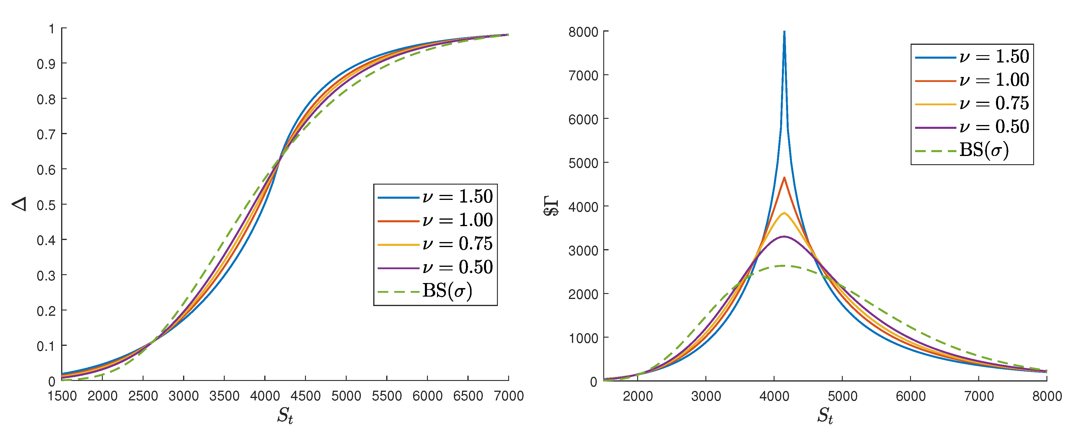
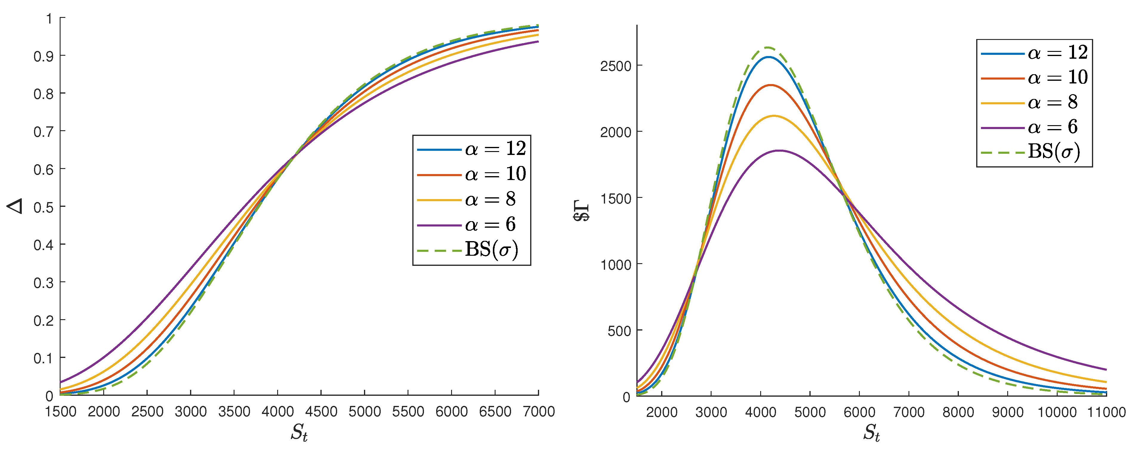
For illustration, in Figure 5 we compare the Delta of VG ( σ , ν , 0 ) while using Formula (2) with that of BS ( σ ) . Similarly, we compare the Dollar Gamma using Formula (3). Figure 6 provides a comparison for NIG ( α , 0 , δ ) . For both models, we can see the substantial impact of the heavy-tailed assumption and its implications for hedging. In the next section, we discuss delta hedging in more detail, and provide some simplified approximations for the ATMF case.

5.1. Delta Hedging

The leading term for the Delta of the European option in the exponential VG case is given for n 1 = n 2 = 1 in (63) and it reads:
Δ V G = F 2 S t Γ ( τ ν ) Γ 1 2 + τ ν 2 Γ ( 3 3 τ ν ) Γ ( 1 2 τ ν ) k V G σ ν 3 + 2 τ ν ;
In the ATMF situation ( S t = F , i.e., k = 0 ), we can re-write the martingale adjustment and Taylor expand for small σ
k V G = ω V G τ = σ 2 2 τ + O σ 4
and, recalling τ ν = τ ν 1 2 , we obtain
Δ V G = 1 2 + O σ 4 ( τ ν + 1 ) .
It is interesting to note that, in the ATMF situation, Δ V G 1 2 , which is, it suffices to be long one unit of the asset S and short two units of an European call written on this asset, to offset the impact of the variations of S on a portfolio; this fact is well-known in the usual Black–Scholes theory, and is therefore preserved in the exponential VG model. The same observation actually also holds for the exponential NIG model: indeed, the leading term in the series (66) (obtained for n 1 = 0 , n 2 = 1 ) reads
F α e α δ τ S t π K 1 2 ( α δ τ ) δ τ 2 α = F 2 S t
where we have used the particular value of the Bessel function of index 1 2 (59) in order to simplify the expression; when F = S t , we obtain Δ N I G = 1 2 , which, again, turns out to be similar to the usual Black–Scholes behavior. This effect is clearly illustrated in Figure 5 and Figure 6. We can conclude that in both the exponential VG and NIG models, the presence of a time subordination does not modify the delta hedging policy, at least when options are not far from the money. In contrast, the option Gamma is significantly influenced by time subordination, and it is discussed further in Section 6.
In the FD model, things are a bit different; keeping only the leading term ( n 1 = n 2 = 0 ) in (67) yields
Δ F D = F α S t S t F 1 α
which explicitly depends on the tail parameter α and resumes to 1 2 in the sub-BS model, for any subordination parameter γ . Again, the subordination parameter plays no role in the delta-hedging policy of the portfolio, which is entirely governed by the tail parameter α ; in other words, it suffices to be long one unit of the underlying asset S and short α European calls to offset the effect of the variations of S on the portfolio’s value.

5.2. Comparisons with Numerical Techniques

In this subsection, we show that the series formulas for the first order sensitivity Δ provided by Formula (2) are a very efficient alternative to Fourier-based computations. Such calculations are typically based on a representation for the price of an European call in terms of Arrau–Debreu securities (see e.g., Lewis (2001))
E Q e r τ ( S T K ) + | S t = S t e q τ Π 1 K e r τ Π 2 ,
where e q τ Π 1 is the option’s Delta. This quantity is known to admit a convenient representation in the Fourier space:
Δ = e q τ Π 1 = 1 2 + 1 π 0 R e e i u k Ψ ˜ ( u i , τ ) i u d u
where k is the log forward moneyness defined in (37), and the “risk-neutralized” characteristic function is defined by:
Ψ ˜ ( u , t ) : = e i u ω t Ψ ( u , t ) = e ( i u ω + ψ ( u ) ) t
In the case of the exponential VG and NIG models, the integral in (74) can be easily carried out by inserting the expressions for the Lévy symbol ψ ( u ) and the martingale adjustment ω , and by evaluating the integral by any classical recursive algorithm (such as a simple trapezoidal rule, for instance). In Table 3, we compare the results of such numerical evaluations, with several truncations of the series in Formula (2), and for various market configurations. We can observe that the convergence is extremely accurate and fast, notably in the ATM region: this is because, in that case, k 0 , which tends to accelerate the overall convergence of the series.

6. Second-Order Sensitivities and Portfolio Performance

6.1. Gamma, Dollar Gamma

The second order derivative of a contingent claim C with respect to S t is often denoted by Γ : = 2 C / S t 2 . It is closely related to the performance, or Profit and Loss (P&L) of a portfolio: if t 2 > t 1 are two trading days, then the P&L between t 1 and t 2 is
P & L = Θ Δ t + market P & L , Δ t : = t 2 t 1 ,
where Θ is the time sensitivity of the portfolio, and the market P&L is, at order 2:
market P & L : = Δ ( Δ S t ) + 1 2 Γ ( Δ S t ) 2 Δ S t : = S t 2 S t 1 .
Assuming that the portfolio has been delta-hedged, then we are left with
market P & L = $ Γ Δ S t S t 2
where the Dollar Gamma has been defined by $ Γ : = 1 2 S t 2 Γ ; relation (78) is widely employed in financial engineering, because it allows for expressing the performance of the portfolio as a simple function of the realized variance of the underlying S. In the usual Black–Scholes theory, it is well known that the Dollar Gamma of the European call is
$ Γ B S = S t 2 σ 2 π τ .
Remarkably, as shown by Formula (3), the Gamma of European options admits a simple form in subordinated market models: while the series expansion for the price or the first-order sensitivity is expressed in terms of a double sum, the Gamma can be expressed as a sum over a single index.
Formula 3
(European call: Gamma).
(i) The Gamma at time t of a European call option in the exponential VG model is:
-
(OTM sensitivity) If k V G < 0 ,
Γ V G ( k V G , σ ν ) = F 2 S t 2 σ ν Γ ( τ ν ) n = 0 ( 1 ) n n ! Γ ( n 2 + τ ν ) Γ ( n + 1 2 ) k V G σ ν n + 2 Γ ( 2 n 2 τ ν ) Γ ( n + 1 2 τ ν ) k V G σ ν 2 n + 2 τ ν .
-
(ITM sensitivity) If k V G > 0 ,
Γ V G + ( k V G , σ ν ) = Γ V G ( k V G , σ ν ) .
-
(ATM sensitivity) If k V G = 0 ,
Γ V G ( k V G , σ ν ) = Γ V G + ( k V G , σ ν ) = F 2 π S t 2 σ ν Γ ( τ ν ) Γ ( τ ν 1 2 ) Γ ( τ ν ) .
(ii) The Gamma at time t of a European call option in the exponential NIG model is:
Γ N I G = F α e α δ τ S t 2 π n = 0 k N I G n n ! Γ ( n + 1 2 ) K n 2 + 1 ( α δ τ ) δ τ 2 α n 2 .
(iii) The Gamma at time t of a European call option in the FD model is:
Γ F D = F α S t 2 n = 0 k F D n n ! Γ ( 1 γ α ( n + 1 ) ) ( ω F D τ γ ) n + 1 α .
Proof. 
The formulas are all straightforward to obtain, by deriving the series in Formula (2) with respect to S t and making an appropriate change of variables. For instance, in the NIG case, we have
Γ N I G = F α e α δ τ S t 2 π n 1 = 0 n 2 = 1 k N I G n 1 n 1 ! Γ ( n 1 + n 2 + 1 2 ) K n 1 n 2 2 + 1 ( α δ τ ) δ τ 2 α n 1 + n 2 2 + n 1 = 1 n 2 = 1 k N I G n 1 1 ( n 1 1 ) ! Γ ( n 1 + n 2 + 1 2 ) K n 1 n 2 2 + 1 ( α δ τ ) δ τ 2 α n 1 + n 2 2 .
Performing the change of variables n ˜ 1 : = n 1 + 1 , n ˜ 2 n 2 + 1 in the second sum shows that only the terms for n ˜ 2 = 0 survive; renaming n ˜ 1 : = n yields Formula (83). □

6.2. Properties and Particular Cases

Let us discuss some useful approximations and qualitative properties of Formula (3). First, in the VG case, the leading term ( n = 0 ) in (80) is
F 2 S t 2 σ ν Γ ( τ ν ) Γ ( τ ν ) π + 2 Γ ( 2 τ ν ) Γ ( 1 2 τ ν ) k V G σ ν 2 τ ν .
Taylor expanding the VG martingale adjustment for small ν and assuming that we are not far from the money forward ( S t F ), we have
k V G ν 0 k σ 2 2 τ S t F σ 2 2 τ ,
therefore, the Gamma writes, at first order:
Γ V G = 1 2 π S t σ ν Γ ( τ ν 1 2 ) Γ ( τ ν )
and the Dollar Gamma immediately follows:
$ Γ V G = S t 4 π σ ν Γ ( τ ν 1 2 ) Γ ( τ ν ) .
While using the functional relation Γ ( z + 1 ) = z Γ ( z ) and the Stirling approximation (47), we have:
Γ ( τ ν 1 2 ) Γ ( τ ν ) = 1 τ ν 1 2 Γ ( τ ν + 1 2 ) Γ ( τ ν ) ν 0 ν τ
and, therefore, we obtain the behavior of (89) in the low variance regime:
$ Γ V G ν 0 S t 2 σ 2 π τ ,
thus recovering the Black–Scholes Dollar Gamma (79) in this limit. It is interesting to note that, contrary to the first order sensitivity Delta (70), which appeared to be independent of ν ; this is no longer the case with the second order sensitivity Gamma (89) that explicitly depends on the subordination parameter. In other words, while the subordination parameter does not modify the Delta Hedging policy of the portfolio (when not far from the money), it directly impacts its performance. This observation also holds in the exponential NIG model; indeed, the leading term in (83) for S t F reads
Γ N I G = α e α δ τ π S t K 1 ( α δ τ )
and therefore the Dollar Gamma is
$ Γ N I G = α S t e α δ τ 2 π K 1 ( α δ τ ) .
Using the asymptotic behavior for large argument (58) for the Bessel function, we know that
K 1 ( α δ τ ) α π 2 α δ τ e α δ τ
and, therefore
$ Γ N I G α S t 2 σ 2 π τ , σ 2 : = δ α ,
recovering the Black–Scholes Dollar Gamma (79). Last in the FD model, the leading term in the series (84) for S t F is
Γ F D = 1 α S t ( ω F D τ γ ) 1 α Γ ( 1 γ α ) ,
and, in the sub-BS model ( α = 2 ), using the approximation (36) for the martingale adjustment,
Γ s u b B S = 1 2 S t Γ ( 1 + 2 γ ) Γ ( 1 γ 2 ) σ τ γ 2 .
Therefore, the Dollar Gamma in the sub-BS model is
$ Γ s u b B S = S t 4 Γ ( 1 + 2 γ ) Γ ( 1 γ 2 ) σ τ γ 2 .
and, in the non fractional limit ( γ 1 ), we have, again,
$ Γ s u b B S γ 1 S t 2 σ 2 π τ .
In Table 4, we summarize these observations, as well as the properties that are discussed for the first-order sensitivity in Section 5.

7. Concluding Remarks

In this article, we have provided a review of several subordinated market models and recalled their main properties. We have also recalled recent formulas while used for European option pricing in this context. Our main conclusions are the following:
(a)
The pricing formulas are smooth and fast converging, and provide excellent agreement with efficient numerical techniques (such as the PROJ method). Moreover, these formulas can provide useful approximations for at-the-money options, and allow for the construction of volatility curves.
(b)
We have derived several analytical formulas for risk sensitivities and shown that they also provide excellent agreement with standard numerical (Fourier) evaluations.
(c)
Thanks to these formulas, we were able to show that the presence of a time subordination in the VG, NIG, and FD models has a minimal impact on the delta hedging policy of an at-the-money option, but, on the contrary, has a direct impact on the P&L of the delta hedged portfolio.
Future work should include extending the pricing and sensitivities formulas to path-dependent instruments or to options written on several assets. It would also be interesting to determine whether these analytical results could be extended if the risk-neutral hypothesis is replaced, for instance, by approaches based on optimal quadratic hedging or utility functions.

Author Contributions

J.-P.A. and J.L.K. performed conceptualization and calculations and prepared the original manuscript draft. J.-P.A., J.L.K. and J.K. reviewed and finalized the manuscript. All authors have read and agreed to the published version of the manuscript.

Funding

J. K. acknowledges support from Grant Agency of the Czech Republic, grant No. 19-16066S, and grant No. 20-17295S.

Conflicts of Interest

The authors declare no conflict of interest.

References

  1. Abramowitz, Milton, and Irene Stegun. 1972. Handbook of Mathematical Functions. Mineola: Dover Publications. [Google Scholar]
  2. Aguilar, Jean-Philippe. 2020a. Some pricing tools for the Variance Gamma model. International Journal of Theoretical and Applied Finance 23: 2050025. [Google Scholar] [CrossRef]
  3. Aguilar, Jean-Philippe. 2020b. Explicit option valuation in the exponential NIG model. arXiv arXiv:2006.04659. [Google Scholar]
  4. Aguilar, Jean-Philippe. 2020c. Pricing Path-Independent Payoffs with Exotic Features in the Fractional Diffusion Model. Fractal Fract 4: 2. [Google Scholar] [CrossRef] [Green Version]
  5. Aguilar, Jean-Philippe, Cyril Coste, and Jan Korbel. 2018. Series representation of the pricing formula for the European option driven by space-time fractional diffusion. Fractional Calculus and Applied Analysis 21: 981–1004. [Google Scholar] [CrossRef] [Green Version]
  6. Andrews, Larry. 1992. Special Functions of Mathematics for Engineers. New York: McGraw & Hill. [Google Scholar]
  7. Barndorff-Nielsen, Ole. 1977. Exponentially decreasing distributions for the logarithm of particle size. Proceedings of the Royal Society of London 353: 401–19. [Google Scholar]
  8. Barndorff-Nielsen, Ole, John Kent, and Michael Sørensen. 1982. Normal Variance-Mean Mixtures and z Distributions. International Statistical Review 50: 145–59. [Google Scholar] [CrossRef]
  9. Barndorff-Nielsen, Ole. 1997. Normal inverse Gaussian distributions and stochastic volatility models. Scandinavian Journal of Statistics 24: 1–133. [Google Scholar] [CrossRef]
  10. Bertoin, Jean. 1999. Subordinators: Examples and Applications. In Lectures on Probability Theory and Statistics. Lecture Notes in Mathematics. Edited by Bernard Pierre. Berlin and Heidelberg: Springer, vol. 1717. [Google Scholar]
  11. Black, Fischer, and Myron Scholes. 1973. The Pricing of Options and Corporate Liabilities. The Journal of Political Economy 81: 637–54. [Google Scholar] [CrossRef] [Green Version]
  12. Bochner, Salomon. 1949. Diffusion equation and stochastic processes. Proceedings of the National Academy of Science of the United States of America 35: 368–70. [Google Scholar]
  13. Boyarchenko, Svetlana, and Sergei Levendorskiĭ. 2000. Option pricing for truncated Lévy Processes. International Journal of Theoretical and Applied Finance 3: 549–52. [Google Scholar] [CrossRef]
  14. Brenner, Menahem, and Marti G. Subrahmanyam. 1994. A simple approach to option valuation and hedging in the Black-Scholes Model. Financial Analysts Journal 50: 25–28. [Google Scholar] [CrossRef]
  15. Calvet, Laurent, and Adlai Fischer. 2008. Multifractal Volatility: Theory, Forecasting and Pricing. Burlington: Academic Press. [Google Scholar]
  16. Carr, Peter, and Dilip Madan. 1999. Option valuation using the Fast Fourier Transform. Journal of Computational Finance 2: 61–73. [Google Scholar] [CrossRef] [Green Version]
  17. Carr, Peter, Hélyette Geman, Dilip Madan, and Marc Yor. 2002. The Fine Structure of Asset Returns: An Empirical Investigation. Journal of Business 75: 305–32. [Google Scholar] [CrossRef] [Green Version]
  18. Carr, Peter, and Liurn Wu. 2003. The Finite Moment Log Stable Process and Option Pricing. The Journal of Finance 58: 753–77. [Google Scholar] [CrossRef] [Green Version]
  19. Carr, Peter, and Liuren Wu. 2004. Time-changed Lévy processes and option pricing. Journal of Financial Economics 71: 113–41. [Google Scholar] [CrossRef] [Green Version]
  20. Cartea, Alavaro, and Diego del-Castillo-Negrete. 2007. Fractional diffusion models of option prices in markets with jumps. Physica A 374: 749–63. [Google Scholar] [CrossRef] [Green Version]
  21. Cont, Rama, and Peter Tankov. 2004. Financial Modelling with Jump Processes. New York: Chapman & Hall. [Google Scholar]
  22. Cont, Rama. 2007. Volatility Clustering in Financial Markets: Empirical Facts and Agent-Based Models. In Long Memory in Economics. Edited by Teyssière Gilles and Kirman Alan. Berlin and Heidelberg: Springer. [Google Scholar]
  23. Clark, Peter K. 1973. A subordinated stochastic process model with fixed variance for speculative prices. Econometrica 41: 135–55. [Google Scholar] [CrossRef]
  24. Cui, Zhenyu, Justin L. Kirkby, and Duy Nguyen. 2017. Equity-linked annuity pricing with cliquet-style guarantees in regime-switching and stochastic volatility models with jumps. Insurance: Mathematics and Economics 74: 46–62. [Google Scholar] [CrossRef]
  25. Cui, Zhenyu, Justin L. Kirkby, and Duy Nguyen. 2019. A general framework for time-changed Markov processes and applications. European Journal of Operational Research 273: 785–800. [Google Scholar] [CrossRef]
  26. de Jonge, Bram, Ruud Teunter, and Tiedo Tinga. 2017. The influence of practical factors on the benefits of condition-based maintenance over time-based maintenance. Reliability Engineering & System Safety 158: 21–30. [Google Scholar]
  27. Eberlein, Ernst, and Ulrich Keller. 1995. Hyperbolic distributions in finance. Bernoulli 1: 281–99. [Google Scholar] [CrossRef]
  28. Eberlein, Ernst, Kathrin Glau, and Antonis Papapantoleon. 2010. Analysis of Fourier Transform Valuation Formulas and Applications. Applied Mathematical Finance 17: 211–40. [Google Scholar] [CrossRef] [Green Version]
  29. Fang, Fang, and Cornelis W. Oosterlee. 2008. A novel pricing method for European options based on Fourier cosine series expansions. SIAM Journal on Scientific Computing 31: 826–48. [Google Scholar] [CrossRef] [Green Version]
  30. Figueroa-López, José E., Steven R. Lancette, Kiseop Lee, and Yanhui Mi. 2012. Estimation of NIG and VG models for high frequency financial data. In Handbook of Modeling High-Frequency Data in Finance. Edited by Viens Frederi, Mariani Maria and Florescu Ionut. Hoboken: John Wiley & Sons. [Google Scholar]
  31. Fiorani, Filippo, Elisa Luciano, and Patrizia Semeraro. 2007. Single and Joint Default in a Structural Model with Purely Discontinuous Assets. Carlo Alberto Notebooks Working Paper 41. Available online: https://EconPapers.repec.org/RePEc:cca:wpaper:41 (accessed on 8 November 2020).
  32. Geman, Hélyette. 2009. Stochastic Clock and Financial Markets. Handbook of Numerical Analysis 15: 649–63. [Google Scholar]
  33. Gorenflo, Rudolf, Francesco Mainardi, and Alessandro Vivoli. 2006. Discrete and Continuous Random Walk Models for Space-Time Fractional Diffusion. Journal of Mathematical Sciences 132: 614–28. [Google Scholar] [CrossRef]
  34. Ivanov, Roman. 2018. Option pricing in the variance-gamma model under the drift jump. International Journal of Theoretical and Applied Finance 21: 1–19. [Google Scholar] [CrossRef]
  35. Jizba, Petr, Jan Korbel, Hynek Lavička, Martin Prokš, Václav Svoboda, and Christian Beck. 2018. Transition between superstatistical regimes: Validity, breakdown and applications. Physica A 493: 29–46. [Google Scholar] [CrossRef] [Green Version]
  36. Kirkby, Justin L. 2015. Efficient Option Pricing by Frame Duality with the Fast Fourier Transform. SIAM Journal on Financial Mathematics 6: 713–47. [Google Scholar] [CrossRef]
  37. Kleinert, Hagen, and Jan Korbel. 2016. Option Pricing Beyond Black-Scholes Based on Double-Fractional Diffusion. Physica A 449: 200–14. [Google Scholar] [CrossRef] [Green Version]
  38. Korbel, Jan, and Yuri Luchko. 2016. Modeling of financial processes with a space-time fractional diffusion equation of varying order. Fractional Calculus and Applied Analysis 19: 1414–33. [Google Scholar] [CrossRef]
  39. Kou, Steven. 2002. A jump-diffusion model for option pricing. Management Science 48: 1086–101. [Google Scholar] [CrossRef] [Green Version]
  40. Krawiecki, Andrzej, Janusz A. Holyst, and Dirk Helbing. 2002. Volatility Clustering and Scaling for Financial Time Series due to Attractor Bubbling. Physical Review Letters 89: 158701. [Google Scholar] [CrossRef] [PubMed] [Green Version]
  41. Lam, Kin, Eric Chang, and Matthew C. Lee. 2002. An empirical test of the variance gamma option pricing model. Pacific-Basin Finance Journal 10: 267–85. [Google Scholar] [CrossRef]
  42. Lewis, Alan. 2001. A Simple Option Formula for General Jump-Diffusion and Other Exponential Lévy Processes. SSRN. SSRN 282110. Available online: https://ssrn.com/abstract=282110 (accessed on 8 November 2020).
  43. Li, Changpin, Deliang Qian, and YangQuan Chen. 2011. On Riemann-Liouville and Caputo Derivatives. Discrete Dynamics in Nature and Society 2011: 562494. [Google Scholar] [CrossRef] [Green Version]
  44. Li, Lingfei, and Vadim Linetsky. 2014. Time-Changed Ornstein-Uhlenbeck processes and their applications in commodity derivative models. Mathematical Finance 24: 289–330. [Google Scholar] [CrossRef] [Green Version]
  45. Linders, Daniel, and Ben Stassen. 2015. The multivariate Variance Gamma model: Basket option pricing and calibration. Quantitative Finance 16: 555–72. [Google Scholar] [CrossRef]
  46. Luchko, Yuri, Jean-Philippe Aguilar, and Jan Korbel. 2019. Applications of the Fractional Diffusion Equation to Option Pricing and Risk Calculations. Mathematics 7: 796. [Google Scholar]
  47. Luciano, Elisa, and Wim Schoutens. 2006. A multivariate jump-driven financial asset model. Quantitative Finance 6: 385–402. [Google Scholar] [CrossRef] [Green Version]
  48. Luciano, Elisa. 2009. Business Time and New Credit Risk Models. Convegno Economia e Incertezza. Available online: https://ideas.repec.org/p/icr/wpmath/16-2010.html#download (accessed on 1 October 2020).
  49. Luciano, Elisa, and Patrizia Semeraro. 2010. Multivariate time changes for Lévy asset models: Characterization and calibration. Journal of Computational and Applied Mathematics 223: 1937–53. [Google Scholar] [CrossRef] [Green Version]
  50. Lux, Thomas, and Michele Marchesi. 2000. Volatility Clustering in Financial Markets: A MicroSimulation of Interacting Agents. International Journal of Theoretical and Applied Finance 3: 675–702. [Google Scholar] [CrossRef]
  51. Madan, Dilip, Peter Carr, and Eric Chang. 1998. The Variance Gamma Process and Option Pricing. European Finance Review 2: 79–105. [Google Scholar] [CrossRef] [Green Version]
  52. Madan, Dilip, and Eugene Seneta. 1990. The Variance Gamma (V.G.) Model for Share Market Returns. The Journal of Business 63: 511–24. [Google Scholar] [CrossRef]
  53. Madan, Dilip, and Elton A. Daal. 2005. An Empirical Examination of the Variance Gamma Model for Foreign Currency Options. The Journal of Business 78: 2121–52. [Google Scholar]
  54. Mainardi, Francesco, Yuri Luchko, and Gianni Pagnini. 2001. The fundamental solution of the space-time fractional diffusion equation. Fractional Calculus and Applied Analysis 4: 153–92. [Google Scholar]
  55. Mandelbrot, Benoit. 1963. The Variation of Certain Speculative Prices. The Journal of Business 36: 384–419. [Google Scholar] [CrossRef]
  56. Merton, Robert. 1976. Option pricing when underlying stock returns are discontinuous. Journal of Financial Economics 3: 125–44. [Google Scholar] [CrossRef] [Green Version]
  57. Mittnik, Svetlozar, and Stefan Rachev. 2000. Stable Paretian Models in Finance. Hoboken: John Wiley & Sons. [Google Scholar]
  58. Niu, Hongli, and Jun Wang. 2013. Volatility clustering and long memory of financial time series and financial price model. Digital Signal Processing 23: 489–98. [Google Scholar] [CrossRef]
  59. Phelan, Carolyn E., Daniele Marazzina, Gianluca Fusai, and Guido Germano. 2019. Hilbert transform, spectral filters and option pricing. Annals of Operations Research 282: 273–98. [Google Scholar] [CrossRef] [Green Version]
  60. Ruijter, Marjon, Mark Versteegh, and Cornelis W. Oosterlee. 2015. On the application of spectral filters in a Fourier option pricing technique. Journal of Computational Finance 19: 76–106. [Google Scholar] [CrossRef] [Green Version]
  61. Rydberg, Tina Hviid. 1997. The Normal inverse Gaussian Lévy process: Simulation and approximation. Communications in Statistics. Stochastic Models 13: 887–910. [Google Scholar] [CrossRef]
  62. Samko, Stefan, Anatoly A. Kilbas, and Oleg Marichev. 1993. Fractional Integrals and Derivatives, Theory and Applications. Yverdon: Gordon and Breach Science Publishers. [Google Scholar]
  63. Sato, Ken-iti. 1999. Lévy Processes and Infinitely Divisible Distributions. Cambridge: Cambridge University Press. [Google Scholar]
  64. Schoutens, Wim. 2003. Lévy Processes in Finance: Pricing Financial Derivatives. Hoboken: Wiley & Sons. [Google Scholar]
  65. Semeraro, Patrizia. 2008. A multivariate Variance Gamma model for financial applications. International Journal of Theoretical and Applied Finance 11: 1–18. [Google Scholar] [CrossRef]
  66. Takahashi, Akihiko, and Akira Yamazaki. 2008. Efficient static replication of European options under exponential Lévy models. The Journal of Futures Markets 29: 1–15. [Google Scholar] [CrossRef] [Green Version]
  67. Tarasov, Vasily E. 2019. On history of mathematical economics: Application of fractional calculus. Mathematics 7: 509. [Google Scholar] [CrossRef] [Green Version]
  68. Tomovski, Živorad, Johan L. A. Dubbeldam, and Jan Korbel. 2020. Applications of Hilfer-Prabhakar operator to option pricing financial model. Fractional Calculus and Applied Analysis 23: 996–1012. [Google Scholar] [CrossRef]
  69. Venter, Johannes, and Riaan de Jongh. 2002. Risk estimation using the Normal inverse Gaussian distribution. The Journal of Risks 2: 1–25. [Google Scholar] [CrossRef]
  70. Zolotarev, Vladimir. 1986. One-dimensional Stable Distributions. Providence: American Mathematical Soc. [Google Scholar]
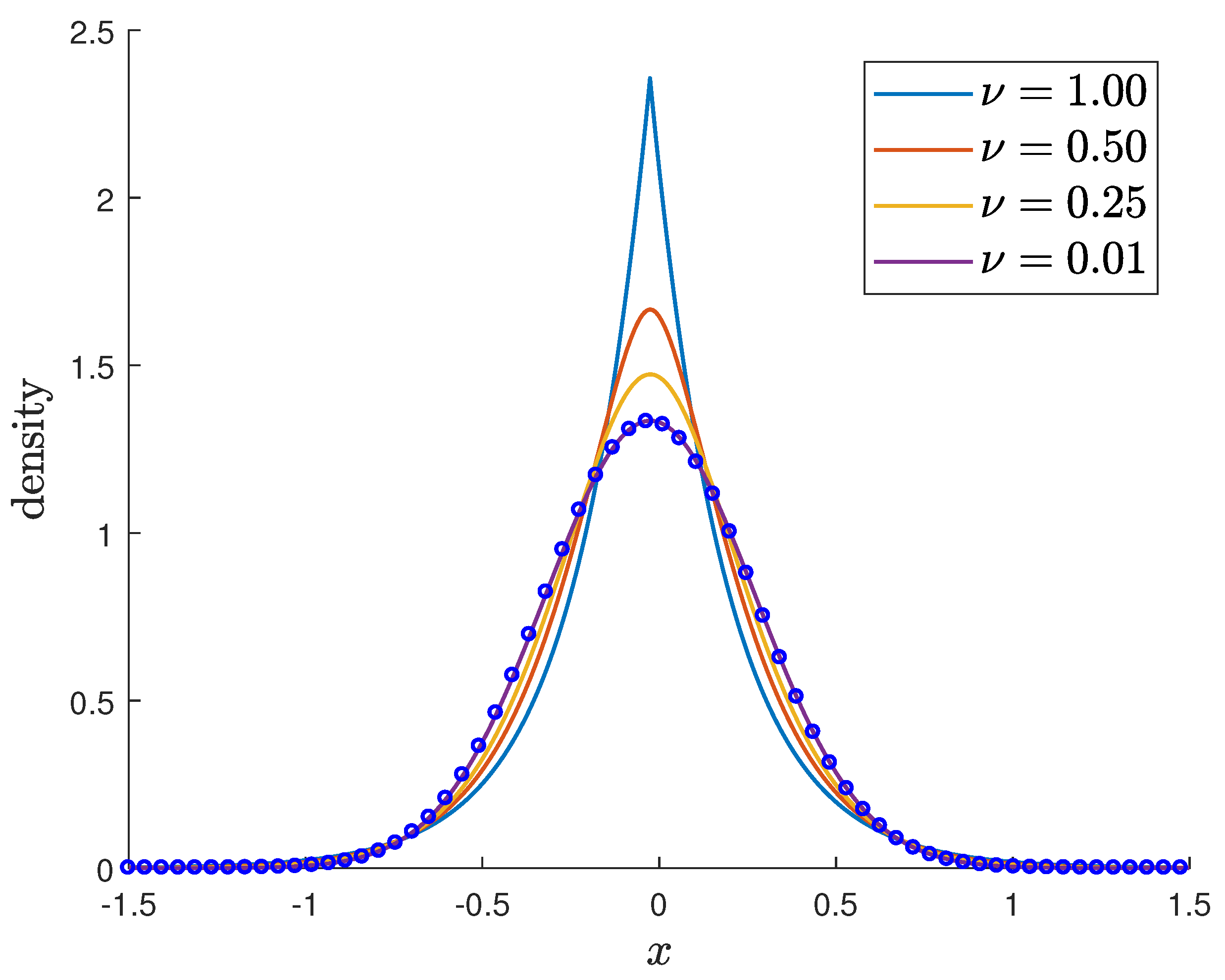
Figure 1. Black–Scholes (circles) as the limit of VG ( σ , ν , 0 ) ν 0 BS ( σ ) .
Risks 08 00124 g001
Figure 2. Log-return densities for several maturities τ , for the VG ( 0.3 , 0.5 , 0 ) model (Left) and the NIG ( 9.0 , 0 , 1.2 ) model (Right).
Risks 08 00124 g002
Figure 3. Exponential convergence of pricing Formula (1) for a call option: τ = 1 , S t = K = 4000 , r = 0.01 , q = 0 . (Left) VG ( σ , ν , 0 ) with σ = 0.3 . (Right) NIG ( α , 0 , δ ) with δ = 1.2 . Here N = n 1 = n 2 is the number of terms in the truncated series.
Risks 08 00124 g003
Figure 4. Implied volatility smiles of VG ( σ , ν , 0 ) obtained by Formula (1). Params: σ = 0.3 , τ = 0.2 , r = 1 % , q = 0 % , S t = 4000 . The moneyness is determined by F : = S t exp ( ( r q ) τ ) .
Risks 08 00124 g004
Figure 5. Delta (Left) and Dollar Gamma (Right) of a call option under VG ( σ , ν , 0 ) using Formula (2) and Formula (3). Greeks of BS ( σ ) are provided for reference (dash lines). Params: σ = 0.3 , τ = 1 , r = 1 % , q = 0 % , K = 4000 .
Risks 08 00124 g005
Figure 6. Delta (Left) and Dollar Gamma (Right) of a call option under NIG ( α , 0 , δ ) using Formulas (2) and (3). Greeks of BS ( σ = 0.3 ) are provided for reference (dash lines). Params: δ = 1.2 , τ = 1 , r = 1 % , q = 0 % , K = 4000 .
Risks 08 00124 g006
Table 1. Some subordinated market models, and their limiting cases. Time changed models (exponential VG and NIG), FD, and sub-BS models recover the Black–Scholes (BS) model for specific values of their subordination parameters.
Subordinated ModelLimiting Regimes
VG ( σ , ν , θ ) VG ( σ , ν , 0 ) ν 0 BS ( σ )
NIG ( α , β , δ ) NIG ( α , 0 , δ ) α BS ( δ / α )
FD ( σ , α , γ ) FD ( σ , α , γ ) γ 1 FMLS ( σ , α ) α 2 BS ( σ )
sub-BS( σ , γ ) : = FD ( σ , 2 , γ ) sub-BS ( σ , γ ) γ 1 BS ( σ )
Table 2. Volatility modelling for ATMF options in various subordinated models, and their limiting cases.
ATMF Implied Volatility (European Options)
Exponential VG σ V G = 2 π ν Γ ( τ ν ) Γ ( 1 2 + τ ν ) C t S t
Low variance regime ( ν 0 ):
σ V G 2 π τ C t S t
Exponential NIGSolve   S t δ τ e α δ τ π K 0 ( α δ τ ) = C t
Large steepness regime ( α ):
δ = 2 π α τ C t 2 S t 2 + 1 4 α τ + O 1 α 2
At order α 0 :
σ N I G : = δ α = 2 π τ C t S t
sub-BS σ F D = 2 Γ ( 1 + 2 γ ) Γ ( 1 + γ 2 ) τ γ 2 C t S t
Non-fractional regime ( γ 1 ):
σ F D 2 π τ C t S t
Table 3. First order sensitivity (Delta) of European call options in the exponential VG and NIG models, obtained by truncations of Formula (2), and by a numerical evaluation of (74). Here, N = n 1 = n 2 is the number of terms in the truncated series. Parameters: K = 4000 , r = 1 % , q = 0 % , τ = 1 .
Exponential VG Model [ σ = 0.2 , ν = 0.85 ]
Formula (2)Lewis (74)
N = 3 N = 5 N = 10 N = 15
Deep OTM ( S t = 3000 )2.18230.63470.09410.09400.0940
OTM ( S t = 3500 )0.41130.25670.24550.24550.2455
ATM ( S t = 4040.90 )0.57030.57180.57190.57190.5719
ITM ( S t = 4500 )0.75690.81130.81340.81340.8134
Deep ITM ( S t = 5000 )0.47290.85890.92060.92060.9206
Exponential NIG Model [ α = 9 , δ = 1 . 2 ]
Formula (2)Lewis (74)
N = 3 N = 5 N = 10 N = 15
Deep OTM ( S t = 3000 )0.29210.27220.27470.27480.2748
OTM ( S t = 3500 )0.42890.43090.43110.43110.4311
ATM ( S t = 4234.09 )0.63360.64100.64120.64120.6412
ITM ( S t = 4500 )0.69360.70300.70330.70330.7033
Deep ITM ( S t = 5000 )0.78270.79660.79710.79710.7971
Table 4. First and second order market sensitivities (ATMF situation) for European call options in various subordinated models, and their limiting cases. Time subordination does not affect the Delta, but it directly impacts the Gamma of options.
1st Order ( Δ )2nd Order ( Γ )
Exponential VG 1 2 1 2 π S t σ ν Γ ( τ ν 1 2 ) Γ ( τ ν )
Low variance regime ( ν 0 ):
1 S t σ 2 π τ
Exponential NIG 1 2 α e α δ τ π S t K 1 ( α δ τ )
Large steepness regime ( α ):
1 S t σ 2 π τ , σ 2 : = δ α
FD 1 α 1 α S t ( ω F D τ γ ) 1 α Γ ( 1 γ α )
sub-BS 1 2 1 2 S t Γ ( 1 + 2 γ ) Γ ( 1 γ 2 ) σ τ γ 2
Non fractional regime ( γ 1 ):
1 S t σ 2 π τ
Publisher’s Note: MDPI stays neutral with regard to jurisdictional claims in published maps and institutional affiliations.