The Importance of Economic Variables on London Real Estate Market: A Random Forest Approach

Abstract

This paper follows the recent literature on real estate price prediction and proposes to take advantage of machine learning techniques to better explain which variables are more important in describing the real estate market evolution. We apply the random forest algorithm on London real estate data and analyze the local variables that influence the interaction between housing demand, supply and price. The variables choice is based on an urban point of view, where the main force driving the market is the interaction between local factors like population growth, net migration, new buildings and net supply.

1. Introduction

Urban economy and real estate markets are two interconnected fields of research. They overlap in so far as the real estate price evolution is analyzed under an urban approach: it has been shown that less than 8% of the variation in price levels across cities can be accounted for by national effects Glaeser et al. (2014), while the remaining part is explained by local factors. In other words, national macroeconomic variables such as population growth, global migration, interest rates or national income, have really tiny power in explaining the real estate market, comparing with the macroeconomic variables accounted at a local level, such as the city population, the migration towards a particular city or the opportunities of jobs in a given urban area, that directly press on built environment and housing demand. On the other hand, the local real estate market influences the urban economy as long as it offers advantageous investment opportunities and facilities able to attract w orkers and economic activities: according to Arvanitidis (2014), the property market institution has a pivotal role through which local economic potential can be realized and served. In this sense, urban economy and real estate market influence each other.

Recently, some phenomena are affecting both urban economy and real estate market evolution. According to the United Nations (2019), the world’s population is expected to grow by 5.9 billion by the end of the century, and about the 80% of which is expected to live in or move toward cities, due to economic and political motivations. Moreover, the population is aging and the proportion of elderly who remains to live in the city is increasing, thanks to alternative pension products based on the property value, like home equity plan and reverse mortgages Di Lorenzo et al. (2020a). In Europe, 25% of the population is already aged 60 years and the proportion who lives in city is growing: by 2050, two-thirds of the world population are expected to live in cities Lopez-Alcala (2016). A complete overview of the urban situation has to take into account data on migration: according to the International Organization of Migration, in 2015 in Europe there have been one million migrants, and many of them stay i n cities McKinsey (2016). As population grows and the urbanization goes on, real estate markets have to face pressure on prices and affordability van Doorn et al. (2019), caused by the mismatch between demand and supply: inflows of people in cities are pressing and asking for new buildings. On the other hand, the increase of working population into metropolitan areas are bearing long-term opportunities for investors. In this context, understanding real estate market evolution is crucial for various real estate stakeholders such as house owners, investors, banks, insurances and other institutional investors like real estate funds. The housing demand is supported by both the need of a house to live in and the research of competitive yields. As highlighted by the emerging trend in Real Estate Europe survey Morrison et al. (2019), real estate has grown as a proportion of the balance sheets of many institutional investors because it has provided the yield and returns that other asset types have not. In particular, in the last decade we have experienced geopolitical uncertainty and decrease in the interest rate and this has reinforced the longing of secure and profitable long-term income. Moreover, many financial intermediaries offer financial and insurance products whose valuation is influenced by the expectation on the real estate market, like mortgages or reverse mortgages Di Lorenzo et al. (2020a). The link between real estate markets and financial market is evident from the recent world economic crisis. Moreover, real estate property represents a major part of the individual wealth Arvanitidis (2014), so it is clear that real estate pricing mechanism is an important driver of the economy.

In light of these considerations, the importance of a precise awareness of the inner workings in the real estate market and an accurate price prediction is evident. The academic literature on this topic is fervent. In order to describe the dynamics of the market and produce predictions, the features that influence the real estate price have to be identified. Gao et al. (2019) grouped these features into two categories: non-geographical factors, that concern the peculiarities of the house, such as the number of bedrooms or the floor space area; and geographical factors, such as the distance to the city center and to main services like the schools. Rahadi et al. (2015) divide the variables explanatory of the house price into three groups: physical conditions, concept and location Chica-Olmo (2007). Physical conditions are properties possessed by the house; the concept concerns internalized ideas of home like minimalist home or healthy and green environment (Ozdenerol et al. 2015; Miller et al. 2009; Coen et al. 2018). Another point of view is the macroeconomic perspective Grum and Govekar (2016), according to which many factors drive the behavior of the real estate market, such as interest rates, government regulation, economic growth, political instability and so on. However, Glaeser et al. (2014) presents an urban approach and show how most variation in housing price changes is local and not national. The empirical evidence confirms that the most important factors driving the value of a house are the size and the location: (Bourassa et al. 2010; Case et al. 2004; Gerek 2014 and Montero et al. 2018) show how different locations have a strong impact on their prices. Spatial location broadly aims to analyze the role of geography and location in economic phenomena, and a particular strand of research is devoted to the analysis of real estate market fluctuations as one of the economic phenomenon in a particular geographic area.

Once the explanatory variables have been chosen, the prediction model has to be identified. The hedonic pricing model has proposed extensively in the literature of house price prediction (Krol 2013; Selim et al. 2009; Del Giudice et al. 2017b). It is essentially used for analyzing the relationship between house price and house features through classical regression methods, assuming that the value of a house is the sum of all its attributes value Liang et al. (2015). Manjula et al. (2017) uses multivariate regression models. Some related works Greenstein et al. (2015) are concerned with trying to estimate the health of a real estate market using the housing index price. Alfiyatin et al. (2017) model house price combine regression analysis and particle swarm optimization. In the last few years, with the diffusion of the application of artificial intelligence in various fields and in the context of real estate Zurada et al. (2011), many authors have used machine learning algorit hms to gain a better fitting of the models. House price predictions have been produced through machine learning (Baldominos et al. 2018; Winson 2018) and deep learning methods, such as artificial neural networks (Nghiep et al. 2001; Selim et al. 2009; Yacim et al. 2016; Yacim et al. 2018; Di Lorenzo et al. 2020b), support vector machine (Gu et al. 2011; Wang et al. 2014) and adaptive boosting Park and Bae (2015). Other contributions deepen the expert systems based on fuzzy logic (Sarip et al. 2016; Del Giudice et al. 2017a; Guan et al. 2008). Guan et al. (2014) propose adaptive neuro-fuzzy inference systems for real estate appraisal. Park and Bae (2015) analyze the problem of classification of an investment in worthy or not, performing different algorithms: decision trees, Naive Bayes and AdaBoost. Manganelli et al. (2007) study the sales of residential property in a city in the Campania region in Italy using linear programming to analyze the real estate da ta. Del Giudice et al. (2017b) predict house price through a Markov chain hybrid Monte Carlo method, and test neural networks, multiple regression analysis and penalized spline semiparametric method. Gao et al. (2019) describe a multi task learning approach to predict location centered house price.

This paper follows the recent developments of the literature on real estate and proposes to take advantage of the random forest algorithm to better explain which variables have more importance in describing the evolution of the house price following an urban approach. To this aim, we focus on a given city, and analyze the local variables that influences the interaction between housing demand and supply and the price. We perform random forest on real estate data of London, that already in the 1990s was attracting literature attention for the economy of its agglomeration Crampton and Evans (1992) and continues to stimulate the international debate for having experienced in the three last decades an extraordinary building boom National Geographic (2018). The novelty of our paper consists in deepening a machine learning (ML) technique for real estate price prediction under an urban approach. In order to achieve this goal, we insert in the algorithm the house price in London as output variable, and some local urban economic variables as input variables. The random forest provides useful support for understanding the relationships between information variables and the target variable and highlighting the importance of each factor. There is a lot of research articles that employ the random forest approach. For instance, it has been considered in early warning systems that signal a country’s vulnerability to financial crises. Tanaka et al. (2016) proposed a novel random forests-based early warning system for predicting bank failures. Tanaka et al. (2019) developed a vulnerability analysis by building bankruptcy models for multiple industries using random forests to predict the probability of firm bankruptcy. Beutel et al. (2019) compared the predictive performance of different machine learning (including random forest) models applied to early warning for systemic banking crises.

In the research concerning real estate, several articles use different ML algorithms to calculate housing prices, such as (Antipov and Pokryshevskaya 2012; Čeh et al. 2018; Hong et al. 2020 and Pai and Wang 2020).

Moreover, we use different explanatory variables with respect to those previously listed. The variables choice is based on an urban point of view, where the main force driving the market is the interaction between local demand and supply, explained by factors like the population growth or the net migration for the demand side, and new buildings and net supply.

The paper is structured as follows. Section 2 describes the regression tree architecture, the random forest technique and the variable importance measure. In Section 3 we present the case study based on the London real estate market. Final remarks are provided in Section 4.

2. The Model

In this section we introduce machine learning techniques for regression problems. In Section 2.1 we briefly describe the regression tree architecture on which the random forest algorithm is based. In Section 2.2 we illustrate the functioning of the random forest and in Section 2.3 we present the variable importance measure used in the case study to catch the importance of each predictor in predicting the target variable.

Machine learning is generally used to perform classification or regression over large datasets. However, it is also proved useful in small datasets to identify hidden patterns that are difficult to detect through more traditional regression techniques such as Generalized Linear Models (GLMs) and Generalized Additive Models (GAMs).

Consider a generic regression problem to estimate the relationship between a target (or response) variable, Y, and a set of predictors (or features), $X_1,X_2,\dots ,X_p$:

$$Y=f(X_1,X_2,\dots ,X_p)+ϵ$$

(1)

where $ϵ$ is the error term. The quantity $E{(Y-\widehat{Y})}^2$ represents the expected squared prediction error. It can rewritten as the sum of the reducible error $E[f(X_1,X_2,\dots ,X_p)$−$\widehat{f}(X_1,X_2,\dots ,X_p){]}^2$ and the irreducible error $Var(ϵ)$. A machine learning technique aims at estimating f by minimizing the reducible error.

Among the machine learning algorithms, we refer to the random forest that falls into the category of the ensemble methods. It allows obtaining the error decrease by reducing the prediction variance, maintaining the bias, which is the difference between the model prediction and the real value of the target variable.

2.1. Regression Tree Architecture

The random forest algorithm is founded on the regression tree architecture. The regression trees enable attaining the best function approximation $\widehat{f}(X_1,X_2,\dots ,X_p)$ through a procedure consisting in the following steps Loh (2011):

• The predictor space (i.e., the set of possible values for $X_1,X_2,\dots ,X_p$) is divided into J distinct and non-overlapping regions, $R_1,R_2,\dots ,R_J$.
• For each observation that falls into the region $R_j$, the algorithm provides the same prediction, which is the mean of the response values for the training observations in $R_j$.

As described in James et al. (2017), the fundamental concept is to split the predictors’ space into rectangles, identifying the regions $R_1,\dots ,R_J$ that minimize the Residual Sum of Squares (RSS):

$$\sum _{j=1}^J\sum _{i\in R_j}{(y_i-{\widehat{y}}_{R_j})}^2$$

Once building the regions $R_1,\dots ,R_J$, the response is predicted for a given test observation using the mean of the training observations in the region to which that test observation appertain.

The consideration of all the possible partitions of the feature is computationally infeasible, thus we use a top-down approach through a recursive binary partition Quinlan (1986): the algorithm starts at the top of the tree, where all values of the target variable stand in a single region, and then successively partitions the predictors’ space. The best split is identified according to the entropy or the index of Gini that is a homogeneity measure for every node. The highest homogeneity (or purity) is achieved when only one class of the target variable is attending the node.

Breiman (2001) has listed the most interesting properties of regression tree-based methods. They belong to non-parametric methods able to catch tricky relations between inputs and outputs, without involving any a-priori assumption. They manage miscellaneous data by applying features selection so as to be robust to not significant or noisy variables. They are also robust to outliers or missing values and easy to be unfolded.

2.2. Random Forest

The random forest (RF) algorithm creates a collection of decision trees from a casually variant of the tree. Once one specific learning set is defined, the RF presents a random perturbation to the learning procedure and in this way a differentiation among the trees is produced. Successively the predictions of all these trees is derived through the impelementation of aggregation techniques. The first aggregation procedure was described by Breiman (1996); the authors proposed the well know bagging based on random bootstrap copies of the original data to assemble different trees. Later in 2001 the same authors Breiman (2001) proposed the random forest as an extention of the procedure of the bagging such that it combines the bootstrap with randomization of the input variables to separate internal nodes t. This means that the algorithm does not identify the best split $s_t=s^{*}$ among all variables, but firstly creates a random subset of K variables for each node and among them determines the best split.

The RF estimator of the target variable ${\widehat{y}}_{R_j}$ is a function of the regression tree estimator, ${\widehat{f}}^{tree}(\mathbf{X})={\sum }_{j\in J}{\widehat{y}}_{R_j}{\mathbf{1}}_{\{\mathbf{X}\in R_j\}}$, where $\mathbf{X}=(X_1,X_2,\dots ,X_p)$ is the vector of the predictors, ${\mathbf{1}}_{\{.\}}$ represents the indicator function and ${(R_j)}_{j\in J}$ are the regions of the predictors space obtained by minimizing RSS. It is identified by the average values of the variable belonging to the same region $R_j$. Therefore, denoting the number of bootstrap samples by B and the decision tree estimator developed on the sample $b\in B$ by ${\widehat{f}}^{tree}(\mathbf{X}|b)$, the RF estimator is defined as follows:

$${\widehat{f}}^{RF}(\mathbf{x})=\frac{1}{B}\sum _{b=1}^B{\widehat{f}}^{tree}(\mathbf{X}|b)$$

(2)

The choice of the number of trees to include in the forest should be done carefully, in order to reach the highest percentage of explained variance and the lowest mean of squared residuals (MSR).

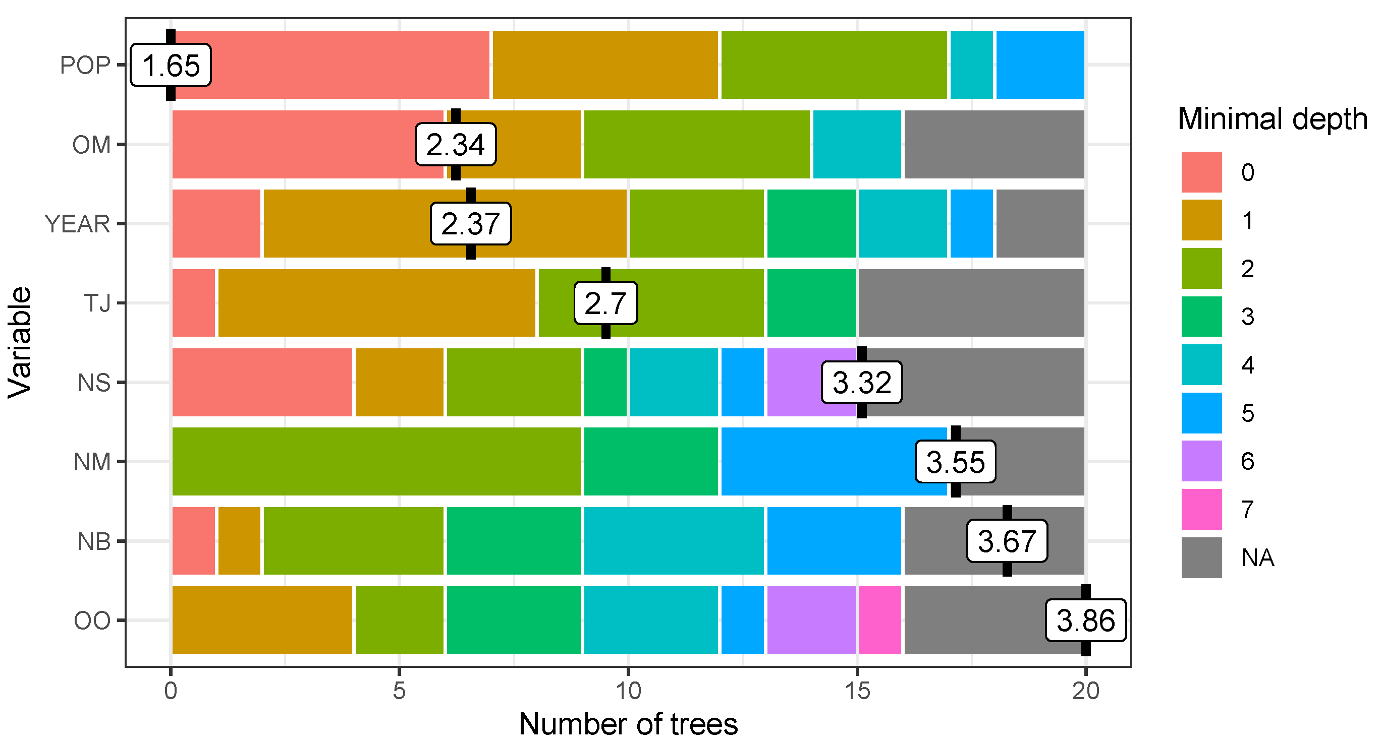
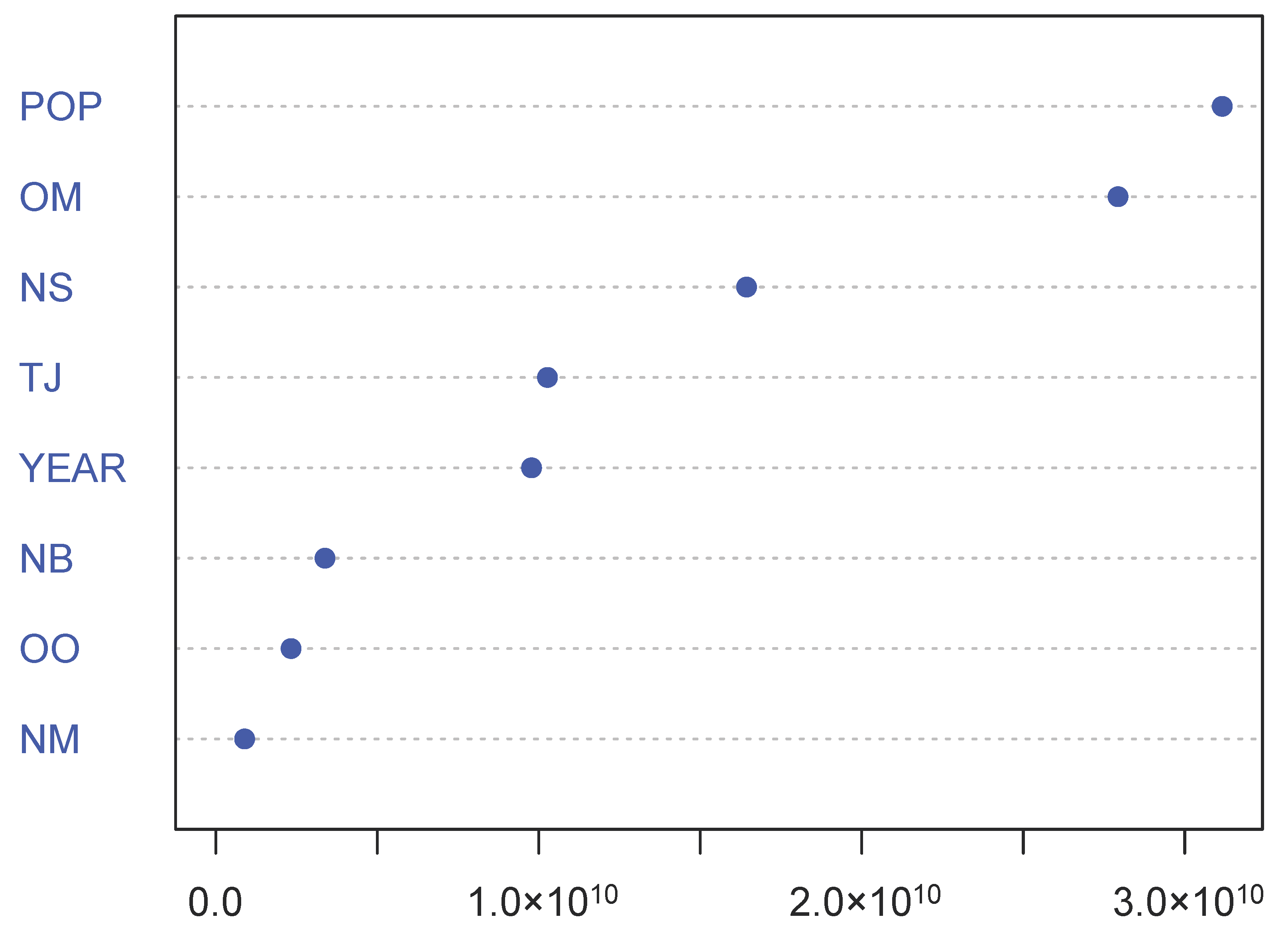
2.3. Variable Importance

ML algorithms are usually viewed as a black-box, as the large number of trees makes the understanding of the prediction rule hard. To get from the algorithm interpretable information on the contribution of different variables we follow the common approach consisting in the calculation of the variable importance measures.

Variable importance is determined according to the relative influence of each predictor, by measuring the number of times a predictor is selected for splitting during the tree building process, weighted by the squared error improvement to the model as a result of each split, and averaged over all trees.

According to the definition provided by Breiman (2001), the RF variable importance is a measure providing the importance of a variable in the RF prediction rule. These measures are often able to detect the interaction effects, i.e., when the predictor variables interact with each other, without any a priori specification Wright et al. (2016).

A weighted impurity measure has been proposed in Breiman (2001) for evaluating the importance of a variable $X_m$ in predicting the target Y, for all nodes t averaged over all $N_T$ trees in the forest. Among the variants of the variable importance measures, we refer to the Gini importance, obtained assigning the Gini index to the impurity $i(t)$ index. This measure is often called Mean Decrease Gini, here denoted by $IncNodePurity$:

$$IncNodePurity(X_m)=\frac{1}{N_T}\sum _T\sum _{t\in T:v(s_t)=X_m}p(t)\Delta i(s_t,t,t_l,t_r)$$

(3)

where $v(s_t)$ is the variable used in split $s_t$ and $\Delta i(s_t,t,t_l,t_r)$ is the impurity decrease of a binary split $s_t$ dividing node t into a left node $t_l$ and a right node $t_r$:

$$\Delta i(s_t,t,t_l,t_r)=i(t)-\frac{N_{t_l}}{N_t}·i(t_l)-\frac{N_{t_r}}{N_t}·i(t_r)$$

(4)

where N is the sample size, $p(t)=\frac{N_t}{N}$ the proportion of samples reaching t, and $p(t_l)=\frac{N_{t_l}}{N}$ and $p(t_r)=\frac{N_{t_r}}{N}$ are the proportion of samples reaching the left node $t_l$ and the right node $t_r$ respectively.

The $IncNodePurity(X_m)$ defined in Equation (3) provides the importance of feature $X_m$, which takes into account the number of splits enclosing the variable. The study of the importance of the feature provides more insight into the learning mode of the algorithm.

3. Case Study

As highlighted in Section 1, in this research we look for the urban explanatory variables of the house price starting from the consideration that the main force driving the market is the interaction between demand and supply. For this reason, we select some local variables that influence the need of house and its the demand, like the population growth or the net migration, and other linked to supply, like new buildings and net supply.

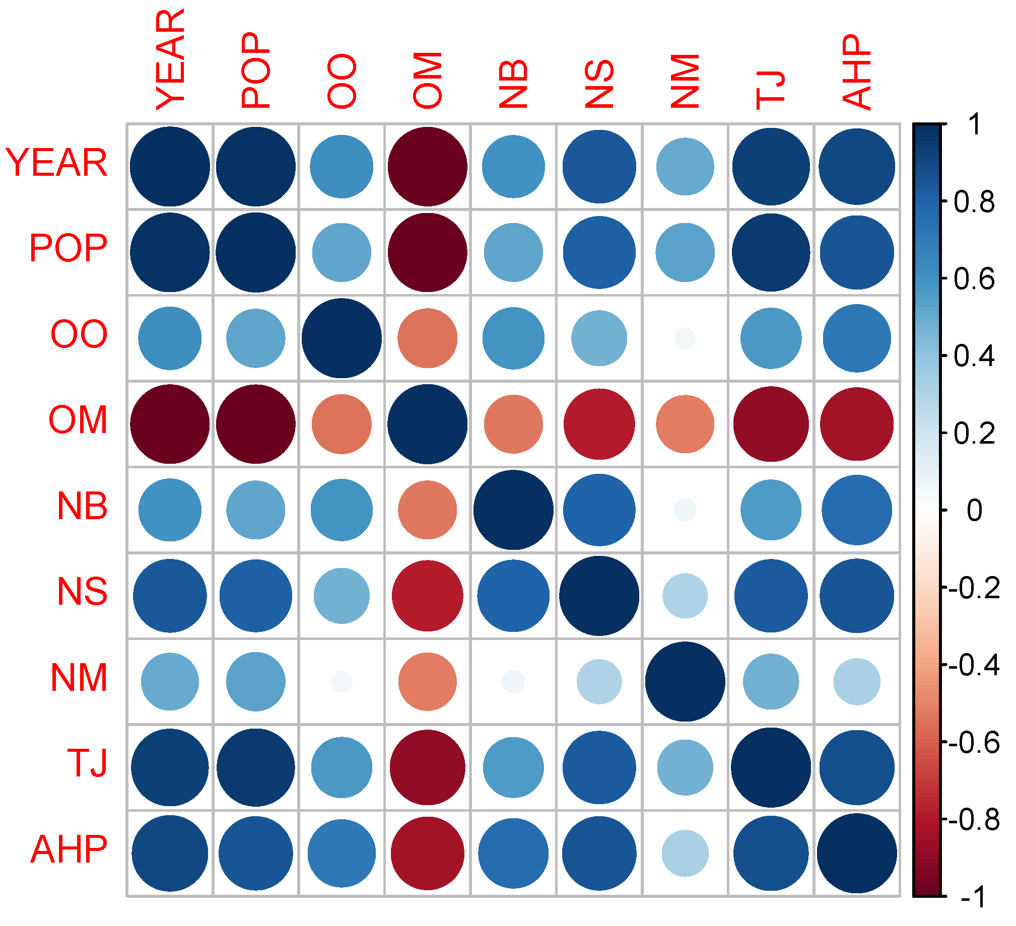
3.1. Data Description

We consider data on survey “Housing in London 2018”, collected by the Greater London Authority City Hall Survey (2018), that provides the average house price (AHP) and the following set of explanatory variables over the period 1997–2016 that are the input of our regression model:

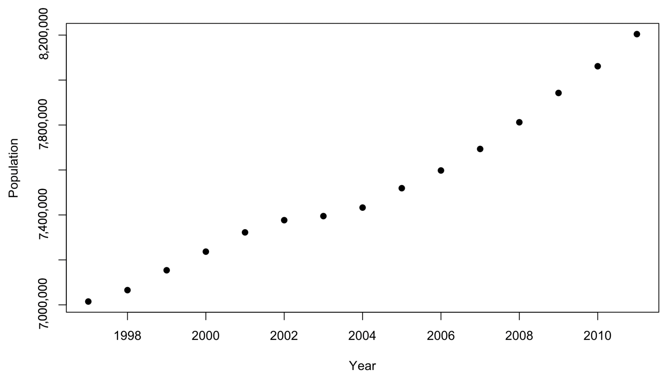
• POP: historic London population
• OO: annual trend in household tenure owned outright
• OM: annual trend in household tenure owned with mortgage
• NB: new build homes
• NS: net housing supply
• NM: net migration (domestic and international)
• TJ: trend of jobs in London

The output variable is the average price across the whole of London. The data considered are purposely generic to highlight the generality of the approach used; it is evident that further ad hoc analyzes can be conducted for individual neighborhoods or areas to obtain more specific results. In this application we are not interested so much in explaining the real estate market of a specific area as in highlighting the results of the application of RF to real estate market. For the precise description of all predictors we refer to Survey (2018).

The Survey (2018) describes the urban situation of London: the London’s population has reached a new peak in 2016, becoming estimated equal to 8.8 million. London’s population boom has been driven by both net international migration and natural change due the annual surplus of births over deaths. Net international migration has risen from around 50,000 a year in 1996 to over 100,000 a year in 2016 and also has explained a part of the increase in natural change, because reducing the average age of London’s population. Moreover net domestic migration has been less volatile than net international migration and has been negative throughout the last 20 years with a net outflow from London equal to 93,000 in 2016. In the same year, more homes than households have been recorded, in contrast to the first half of the 20th century, because the number of people for every home has risen, while falling across the rest of the country. We are attending the declining share of mortgagors for ho me ownership and the growth in people living in a shared private rented home. The number of homes built in London in 2017 is the highest since 1977, but in the same time the population is projected to be equal to 10.5 in 2035, so two thirds of Londoners say they would support new homes being built. Another aspect that detects the home demand is its composition, that is changing: the proportion of households that own their home with a mortgage fell from 38% in 2000 to 29% in 2011, while the proportion that rent privately rose from 15% to 25%. In particular, in 2017 22% of households in London owned their home outright, 29% had a mortgage, 27% rented privately and 21% were in social housing. Another factor that has influenced the urbanization of London has been its flourishing economy. Since 1997, both London’s population and economy have grown consistently. In the last two decades, the number of jobs in London grew by 42%, while the population grew by 26%. However, this rap id economic and demographic growth was not matched by an increase in the housing stock: the new buildings have increased the number of homes by 16% over the same period. The constructions of new buildings are expected to further increase to satisfy the growing demand.

3.2. Regression Model and Main Statistics

In order to understand how this scenario influences the house price, the regression problem is then formulated as follows:

$$\mathrm{AHP}\sim \mathrm{YEAR}+\mathrm{POP}+\mathrm{OO}+\mathrm{OM}+\mathrm{NB}+\mathrm{NS}+\mathrm{NM}+\mathrm{TJ}$$

(5)

Table 1. Summary statistics across years 1997–2016.

Variable	Summary Statistics
POP	$\mu$ = 7,776,538.90	$\sigma$ = 554,808	CV = 7.13%
OO	$\mu$ = 21.56	$\sigma$ = 1.00	CV = 4.64%
OM	$\mu$ = 33.33	$\sigma$ = 3.96	CV = 11.88%
NB	$\mu$ = 18,385.00	$\sigma$ = 3695.46	CV = 20.10%
NS	$\mu$ = 27,314.00	$\sigma$ = 7929.26	CV = 29.03%
NM	$\mu$ = 23,752.40	$\sigma$ = 24,129.15	CV = 101.59%
TJ	$\mu$ = 4,857,200.00	$\sigma$ = 424,621.52	CV = 8.74%
AHP	$\mu$ = 320,045.95	$\sigma$ = 89,380.52	CV = 27.93%

shows the summary statistics for the input variables in the data. In addition to mean ($\mu$) and standard deviation ($\sigma$), we also show the coefficient of variation (CV), or relative standard deviation, that is a standardized measure of dispersion of frequency distribution. It shows the extent of variability in relation to the mean of the average house price ($cv=\frac{\sigma }{\mu }$).

In addition, we show in Figure 1 a graphical display of the correlation matrix. Positive correlations are depicted in blue and negative correlations in red color. The color intensity and the size of the circle are proportional to the correlation coefficients. We observe strong correlations between some of the features. The average house price (AHP) is positively strongly correlated with YEAR and then with the population (POP) and trend of jobs (TJ) while it is negatively correlated with the annual trend in household tenure—owned with mortgage (OM). Moreover, POP is in turn positively correlated with TJ and YEAR and negatively correlated with OM.

3.3. RF Estimation of $AHP$

We solve Equation (5) through the random forest algorithm presented in Section 2. We denote $\widehat{\mathrm{AHP}}$ the random forest estimator, obtained by applying the random forest algorithm implemented in the R package randomForest Liaw (2018) to the London average house prices.

A machine learning algorithm provides different outcomes when changing the seed and the number of trees. Therefore, we initially consider a set of 1000 random seeds for the pseudo-random generator used in the RF algorithm, as well as a set of reasonable number of trees (≤50) and we choose the combination of seed/number of trees producing the lowest mean of squared residuals, MSR. This allows to obtain a high percentage of variance explained and avoid model’s over-fitting. Therefore, the algorithm’s parameters have been set as follows: number of trees (ntrees) equal to 21 and the number of input variables to be used in each node (mtry) equal to 3. The percentage of variance explained by the random forest algorithm, RSS, and the level of MSR resulting from the application of the RF algorithm to the dataset are given in

Table 2. Residual Sum of Squares (RSS) and mean of squared residuals (MSR) by the random forest algorithm. Years 1997–2016.

Indicator	Value
RSS	94.01%
MSR	454,451,969

.

In order to find the best model explaining our data, we have to balance bias and variance. Models with high bias simplify the relationship between target variable and predictors, providing a high error on both training and test set. Meanwhile, models with high variance, focusing too much on the training set, lose the generalization capacity providing a very low error on the training set and very high error on the test set. Models trained on small datasets could result in high variance and high error on the test set, giving rise to overfitting. This can be avoided by reducing the maximum depth so improving the model’s ability to disregard patterns that do not exist. To this purpose, we calculate the distribution of the mean minimal depth, illustrated in Figure 2. The mean value placed at the vertical bar indicates the mean minimal depth: the smaller its value, the more important the variable is. The rainbow gradient provides the minimum and maximum minimal depth for each predictor. The higher the width of red blocks, more frequently the variable is the root of a tree. As missing values appears when a feature is not used for tree splitting, the higher the width gray blocks, less frequently the variable is used for splitting trees.

The values of the mean decrease Gini of features attributed by the algorithm, in descending order from top to bottom, are depicted in Figure 3. It allows to identify which predictor are the most important to understand the underlying process that is the average house price. Despite the decline in the proportion of households that own their home with a mortgage Survey (2018), the annual trend in household tenure owned with mortgage (OM) is the one of most explanatory variables of the house price between those selected. Quite the opposite, annual trend in household tenure owned outright (OO) is one of the less important variable, supporting by the data according to which the proportion of households owned their home outright is very low. We can note that RF algorithm selects POP as the most explicative variable, but since it is strongly positively correlated with YEAR the two variables have the same explicative power in the description of the output. Consequently, the algorithm includes just one of these latter variables among those having a greater importance. Instead, since POP and OM are negatively correlated, they offer different information in the prediction of AHP, so they are both selected as important.

Figure 4 shows the marginal effect of the three most important predictors on the the target variable averaged over the joint values of the other predictors. These plots are called partial dependence plots. We show the effect of the population, annual trend in household tenure—owned with mortgage and net housing supply on the London average house price.

All these variables clearly show non-linear pattern, further confirming the choice of the RF model. In fact, in case of linear pattern a simple linear (or logistic for binary target variables) regression model should be preferable to more complex ones. While, if the data shows non-linear and irregular pattern, like in our dataset, then random forest can be widely considered a very good choice, as we will demonstrate in the following.

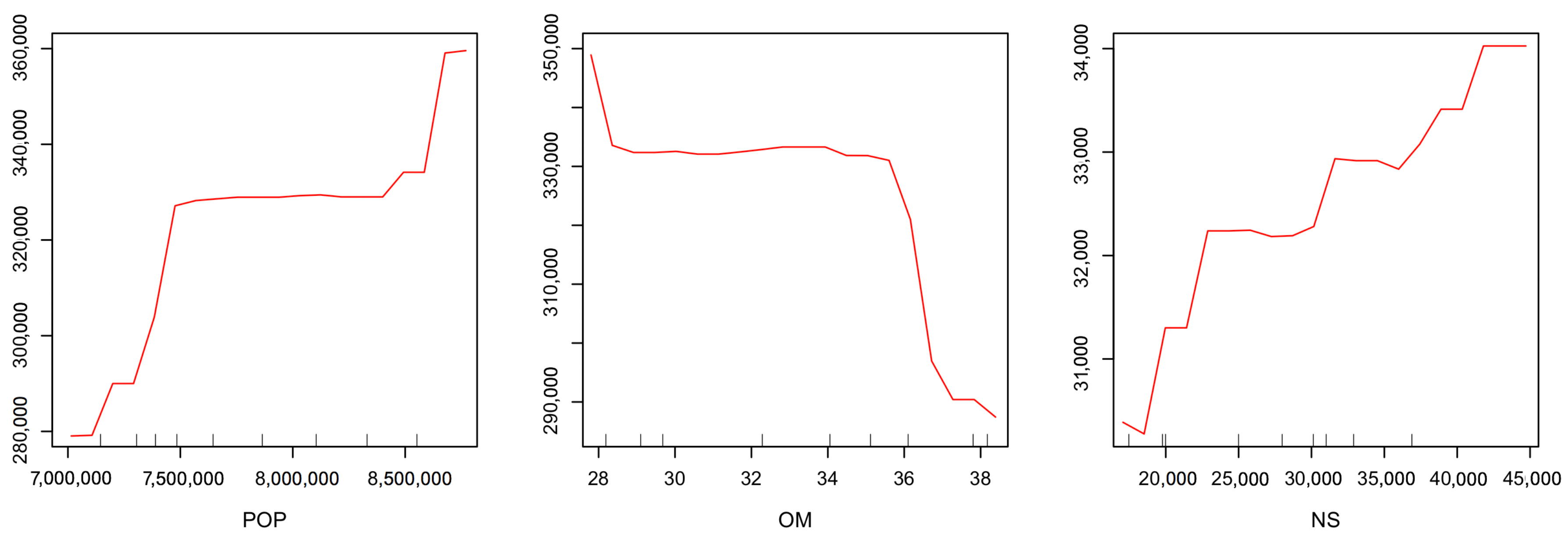
3.4. Sensitivity to Predictor

As shown in the previous sub-section, the $IncNodePurity$, measuring the importance of the variables, provides the highest value of node purity for POP, which therefore represents the most important variable in the RF (Figure 3). In this sub-section we perform a predictors sensitivity analysis by progressively adding one predictor in modeling $\widehat{\mathrm{AHP}}$, aiming at measuring the contribution of each predictor to refine the model accuracy. Then, we combine the selected predictors two by two. We consider the first three predictors in terms of importance.

Table 3. RF estimation of $\widehat{\mathrm{AHP}}$ according to different predictors.

YEAR	POP	OM	NS	POP + OM	POP + NS	OM + NS	Obs.
1997	183,781	177,594	220,706	177,349	199,614	202,211	149,616
1998	193,924	173,391	225,909	157,184	214,491	198,730	170,720
1999	211,542	212,472	208,978	198,043	202,130	229,106	179,888
2000	217,570	178,742	201,503	203,084	195,192	187,088	217,691
2001	236,617	205,580	199,442	237,029	228,907	208,593	243,062
2002	264,721	317,158	190,907	328,907	254,313	273,101	272,549
2003	271,452	301,789	215,949	275,967	261,350	262,067	322,936
2004	331,517	342,420	354,699	339,730	352,269	342,233	332,406
2005	348,727	334,189	346,321	331,844	341,708	332,266	342,173
2006	346,830	347,434	349,716	353,006	352,616	339,709	344,887
2007	343,530	351,773	377,760	354,995	377,016	368,037	369,225
2008	361,114	363,370	373,558	359,544	357,437	354,736	395,803
2009	364,396	365,626	350,713	355,699	349,910	353,876	335,008
2010	352,958	345,881	344,328	343,831	341,911	340,788	357,004
2011	351,097	346,328	340,926	348,378	339,996	354,018	349,730

shows the values of $\widehat{\mathrm{AHP}}$ obtained by RF algorithm in a regression model based on one/two predictors. While, Figure 5 reports the residuals of these models. Looking at the panels with POP, NS, POP + NS and OM + NS predictors, the highest values of residuals correspond to years 1997 and 2003, when the London population data show two inflection points (Figure 6).

As shown in

Table 4. RF estimation of $\widehat{\mathrm{AHP}}$ according to different predictors: % of explained variance (RSS).

Predictor	RSS
POP	91.29%
OM	86.74%
NS	69.08%
POP + OM	87.53%
POP + NS	84.77%
OM + NS	82.41%

, the results of RF prediction confirm that $POP$ is the most explicative feature with a percentage of explained variance (RSS) equal to 91.29%, followed by $OM$ with 86.74%.

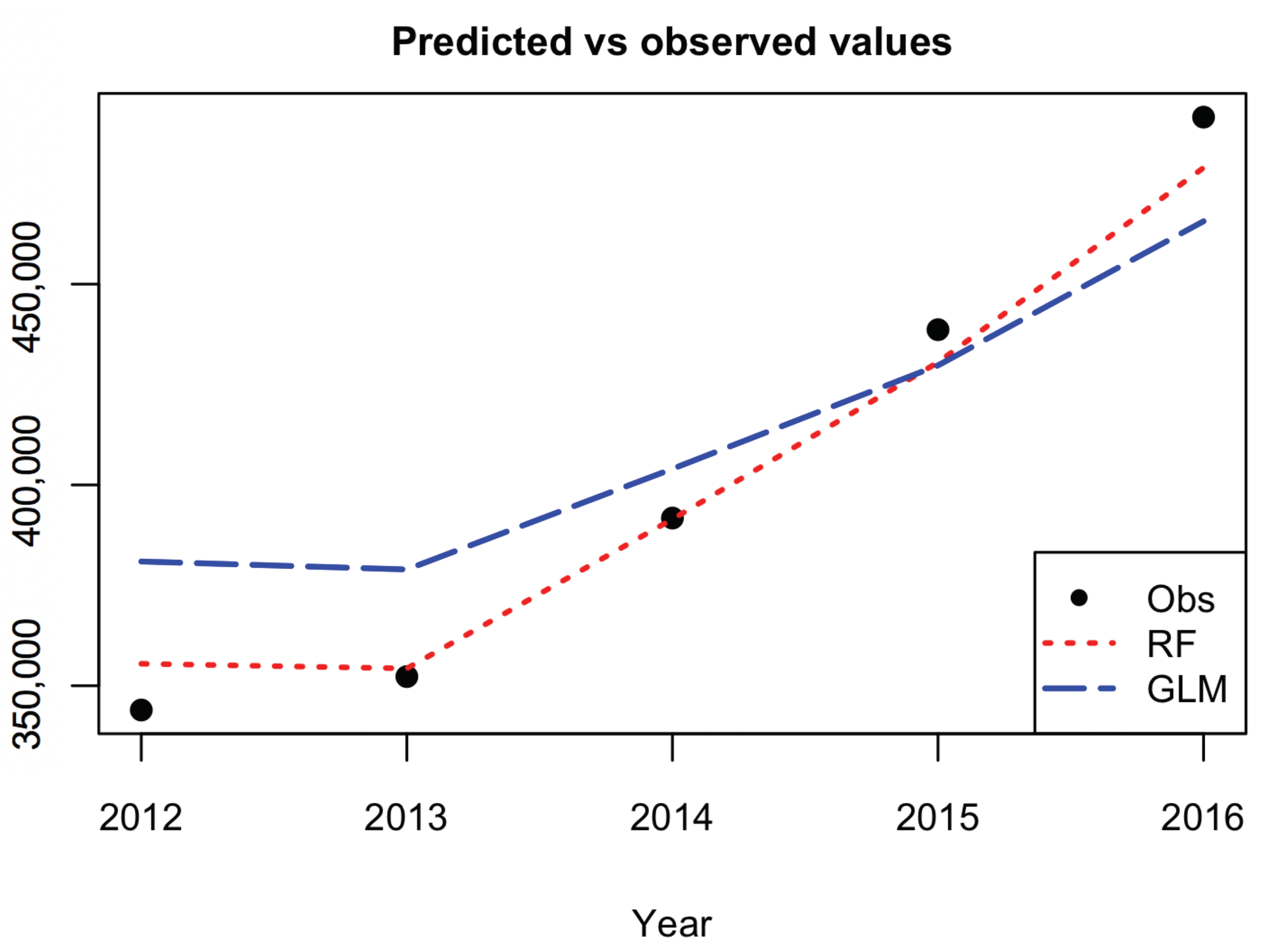
3.5. RF Predictive Performance and Comparison with GLM

To perform the prediction we partition the dataset into training set (1997–2011) and testing set (2012–2016). The data have been randomly partitioned, however there are a set of popular data splitting methods that could potentially work well with alternative data. Among them, cross-validation (CC)1, bootstrapping, bootstrapped Latin partition, Kennard-Stone algorithm (KS) and sample set partitioning based on joint X-Y distances algorithm (SPXY) (see e.g., Xu and Goodacre (2018) for further details).

The ability of the RF algorithm to predict the average house price according to our sample is compared to the performance of a GLM.

In a GLM, the explanatory variables, $\mathbf{X}=(X_1,X_2,\dots ,X_p)$, are related to the response variable, Y, via a link function, $g()$. Denoting $\eta =g(E(Y))$ the linear predictor, the following equation describes how the mean of the response variable depends on the linear predictor:

$$\eta ={\beta }_0+{\beta }_1{X}_1+\cdots +{\beta }_p{X}_p$$

(6)

where ${\beta }_1,\dots ,{\beta }_p$ are the regression coefficients that need to be estimated and ${\beta }_0$ is the intercept. We assume a Gaussian distribution for Y and an identity for the link function, so that: $\eta =E(Y)$. To assess the importance of variables, we measure the significance of the predictors by the Wald test with the null hypothesis: $H_0:\beta =0$. The GLM performance and the estimate of the regression coefficients are reported in

Table 5. GLM results.

Coefficient	$\widehat{\mathit{\beta }}$	$\mathit{SE}(\widehat{\mathit{\beta }})$	z Value	$\mathit{Pr}(>|\mathit{z}|)$
(Intercept)	$-1.004\times {10}^8$	$3.099\times {10}^7$	$-3.239$	0.00789 **
YEAR	$5.092\times {10}^4$	$1.542\times {10}^4$	3.302	0.00705 **
POP	$-2.961\times {10}^{-1}$	$1.932\times {10}^{-1}$	$-1.533$	0.15363
OO	$-1.094\times {10}^4$	$1.240\times {10}^4$	$-0.882$	0.39640
OM	$1.972\times {10}^4$	$2.287\times {10}^4$	0.862	0.40706
NB	1.606	3.738	0.430	0.67569
NS	$-8.192\times {10}^{-1}$	2.453	$-0.334$	0.74467
NM	$-4.009\times {10}^{-1}$	$3.267\times {10}^{-1}$	$-1.227$	0.24538
TJ	$8.134\times {10}^{-2}$	$1.138\times {10}^{-1}$	0.715	0.48958

Significance codes: p < 0.1, ** p < 0.01.

, where $z=\frac{\widehat{\beta }}{SE(\widehat{\beta })}$ is the value of the Wald test, $Pr(>|z|)$ is the corresponding p-value, and $SE(\widehat{\beta })$ is the standard error of the model.

Apart from the intercept, the GLM assigns the greatest importance to the predictor YEAR. This result differs from that obtained through the RF algorithm, which ascribes greater importance to the variables population and household tenure owned with mortgage (POP and OM).

We measure the goodness of prediction through the root mean square error (RMSE) and mean absolute percent error (MAPE), respectively defined as:

$$RMSE=\frac{{\sum }_i{(y_i-{\widehat{y}}_i)}^2}{n}$$

(7)

$$MAPE=\frac{100}{N}\sum _i\left|\frac{y_i-{\widehat{y}}_i}{y_i}\right|$$

(8)

The resulting values of RMSE and MAPE are shown in

Table 6. RMSE and MAPE on predicted values, years 2012–2016.

Measure	RF	GLM
RMSE	8505	24,416
MAPE	1.68%	5.75%

for RF and GLM: the improvement in the prediction obtained by applying RF with respect to the traditional GLM is strong, reducing the MAPE from 5.75% to 1.68%.

Figure 7 illustrates the predicted average house prices obtained by the random forest algorithm compared to the values predicted by GLM. We can observe that GLM overestimates the AHP values in the period 2012–2014 and underestimates them in 2015–2016. The RF algorithm turns out to be more flexible, characterized by a better adaptive capacity.

In addition, we apply the Diebold–Mariano test (Diebold and Mariano 1995) for comparing the accuracy of forecast performance between $RF$ and $GLM$. We define the forecast error $e_{it}$ as:

$$e_{it}={\widehat{y}}_{it}-y_{t}i=1,2$$

(9)

where ${\widehat{y}}_{it}$ and $y_t$ are the predicted and actual values at time t, respectively. The loss associated with forecast i is assumed to be a function of the forecast error and is denoted by $g(e_{it})$. We assume $g(e_{it})=e_{it}^2$. The two forecasts have equal accuracy if and only if the loss differential between the two forecasts, $d_t=g(e_{1t})-g(e_{2t})$, has zero expectation for all t.

The DM test statistic is defined as follows:

$$DM=\frac{\overline{d}}{\sqrt{\frac{s}{N}}}$$

(10)

where $\overline{d}$ is the sample mean of the loss differential, s is the variance, and N the sample size. The null hypothesis of this test is that the models have the same forecast accuracy, i.e., $H_0:E[d_t]=0,\forall t$, while the alternative hypothesis is that $H_1:E[d_t]\ne 0,\forall t$. If $H_0$ is true, then the $DM$ statistic is asymptotically distributed as a normal standard normal distribution with 0 mean and standard deviation equal to 1.

According to the $DM$ test, since $DM=-2.416$ with p-value = 0.0365, the null hypothesis is rejected at the 5% level of significance, indicating that the observed differences between RF and GLM are significant and the forecasting accuracy of RF is better than that of GLM.

At the end of this section we briefly focus on a problem often ignored by the literature: the endogeneity of predictors that produces bias in the forecast results of regression algorithms. In our case, for instance, newly built homes may certainly affect home prices, but also the opposite could be true as well. The endogeneity could generate bias in the regression models and impacts on statistical significance of the coefficients. In the ordinary least square regression the bootstrapping method is used to reduce the bias of the coefficients. However, nonlinear methods in machine learning cannot provide coefficients of each feature, and thus it is not possible to bias correct the nonlinear regression. Recently, to overcome this problem Ghosal (2018) develop the one-step boost random forest for bias correction.

4. Conclusions

In this paper we have implemented a machine learning algorithm, RF, to predict houses price with an application to UK real estate data. In particular, we have analyzed the average house price of the center of London, taking in consideration urban explicative variables of the demand and supply of the houses. The point of view offered is different and complementary with respect to the literature on the field, which considers features attaining the buildings like size and location, and is based on an urban perspective to explain the evolution of the local real estate market. This is the main reason our data set has been selected. Despite the dataset size being small, the numerical results show a better prediction improvement by RF with respect to the traditional regression approach based on GLM. The use of RF in small datasets is common among data scientists as the bootstrapping, on which RF is based, allows the algorithm to perform well anyway. RF is relatively easy to build and does not require expensive hyperparameters tuning. Besides, to avoid overfitting that generally affects the models trained on small datasets, we control both the number of trees and the maximum depth. This improves the model’s ability to do not see patterns that do not exist. As regard to the importance of variables, the algorithm selects the local population as the most predictive variable. This result confirms that the demand size is the main driver of the real estate market. The space for further works is twofold: on one hand the model presented is flexible and can be easily extended to combine variables related to supply and demand with others attaining to the physical features of the house, on the other hand, different machine learning algorithms, like that deals with the problem of the endogeneity of predictors and the bias of results, can be implemented and compared. The research conducted can be reproduced for the analysis of other real estate dataset. A more accurate forecast of the evolution of real estate market prices must exploit not only variables relating to local characteristics of the market, but also combine them with different information sources such as macroeconomic ones. The improvements achieved can show practical feedback for the whole society. As population and urbanization grow, the need for models able to catch the possible evolution of the real estate market concerns more stakeholders, from homeowners to real estate companies to insurance companies and so on. In modern society we are witnessing the growth of the elderly “cash poor house rich”, those who own a home but have retirement incomes so low that they cannot ensure a decent survival and the necessary medical care. Faced with this phenomenon, the insurance market of Reverse Mortgage is developing considerably. In this context, the role that data play will be at the core of the forecasting of assets future value in terms of real-world evaluation and of the cost of insurance contracts related to house valuation.

References

1. Alfiyatin, Adyan Nur, Ruth Ema Febrita, Hilman Taufiq, and Wayan Firdaus Mahmudy. 2017. Modeling House Price Prediction using Regression Analysis and Particle Swarm Optimization Case Study: Malang, East Java, Indonesia. International Journal of Advanced Computer Science and Applications 8. [Google Scholar] [CrossRef] [Green Version]
2. Antipov, Evgeny A., and Elena B. Pokryshevskaya. 2012. Mass appraisal of residential apartments: An application of Random forest for valuation and a CART-based approach for model diagnostics. Expert Systems with Applications 39: 1772–78. [Google Scholar] [CrossRef] [Green Version]
3. Arvanitidis, Pachalis A. 2014. The Economics of Urban Property Markets: An Institutional Economics Analysis. Series: Routledge Studies in the European Economy; London and New York: Routledge, Taylor & Francis Group, ISBN 9780415426824. [Google Scholar]
4. Baldominos, Alejandro, Ivan Blanco, Antonio José Moreno, Rubén Iturrarte, Oscar Bernardez, and Carlos Alfonso. 2018. Identifying Real Estate Opportunities Using Machine Learning. Applied Science 8: 2321. [Google Scholar] [CrossRef] [Green Version]
5. Beutel, Johannes, Sophia List, and Gregor von Schweinitz. 2019. Does machine learning help us predict banking crises? Journal of Financial Stability 45. [Google Scholar] [CrossRef]
6. Bourassa, Steven C., Eva Cantoni, and Martin Hoesli. 2010. Predicting house prices with spatial dependence: A comparison of alternative methods. Journal of Real Estate Research 32: 139–59. [Google Scholar]
7. Breiman, Leo. 1996. Bagging predictors. Machine Learning 24: 123–40. [Google Scholar] [CrossRef] [Green Version]
8. Breiman, Leo. 2001. Random forests. Machine Learning 45: 5–32. [Google Scholar] [CrossRef] [Green Version]
9. Case, Bradford, John Clapp, Robin Dubin, and Mauricio Rodriguez. 2004. Modeling spatial and temporal house price patterns: A comparison of four models. The Journal of Real Estate Finance and Economics 29: 167–91. [Google Scholar] [CrossRef]
10. Čeh, Marian, Milan Kilibarda, Anka Lisec, and Branislav Bajat. 2018. Estimating the Performance of Random Forest versus Multiple Regression for Predicting Prices of the Apartments. ISPRS International Journal of Geo-Information 7: 168. [Google Scholar] [CrossRef] [Green Version]
11. Chica-Olmo, Jorge. 2007. Prediction of Housing Location Price by a Multivariate Spatial Method. Cokriging, Journal of Real Estate Research 29: 91–114. [Google Scholar]
12. Coen, Alan, Patrick Lecomte, and Dorra Abdelmoula. 2018. The Financial Performance of Green Reits Revisited. Journal of Real Estate Portfolio Management 24: 95–105. [Google Scholar] [CrossRef]
13. Crampton, Graham, and Alan Evans. 1992. The economy of an agglomeration: The case of London. Urban Studies 29: 259–71. [Google Scholar] [CrossRef]
14. Del Giudice, Vincenzo, Pierfrancesco de Paola, and Giovanni Battista Cantisani. 2017a. Valuation of Real Estate Investments through Fuzzy Logic. Buildings 7: 26. [Google Scholar] [CrossRef]
15. Del Giudice, Vincenzo, Benedetto Manganelli, and Pierfrancesco de Paola. 2017b. Hedonic analysis of housing sales prices with semiparametric methods. International Journal of Agricoltural and Environmental Information System 8: 65–77. [Google Scholar] [CrossRef] [Green Version]
16. Diebold, Francis X., and Roberto S. Mariano. 1995. Comparing Predictive Accuracy. Journal of Business and Economic Statistics 13: 253–63. [Google Scholar]
17. Di Lorenzo, Emilia, Gabriella Piscopo, Marilena Sibillo, and Roberto Tizzano. 2020a. Reverse Mortgages: Risks and Opportunities. In Demography of Population Health, Aging and Health Expenditures. Edited by Christos Skiadas and Charilaos Skiadas. Springer Series on Demographic Methods and Population Analysis; Cham: Springer, pp. 435–42. ISBN 978-3-030-44695-6. [Google Scholar]
18. Di Lorenzo, Emilia, Gabriella Piscopo, Marilena Sibillo, and Roberto Tizzano. 2020b. Reverse mortgages through artificial intelligence: New opportunities for the actuaries. Decision in Economics and Finance. [Google Scholar] [CrossRef]
19. Gao, Guangliang, Zhifeng Bao, Jie Cao, A. K. Quin, and Timos Sellis. 2019. Location Centered House Price Prediction: A Multi-Task Learning Approach. arXiv arXiv:1901.01774. [Google Scholar]
20. Gerek, Ibrahim Halil. 2014. House selling price assessment using two different adaptive neuro fuzzy techniques. Automation in Construction 41: 33–39. [Google Scholar] [CrossRef]
21. Ghosal, Indrayudh, and Giles Hooker. 2018. Boosting random forests to reduce bias; One step boosted forest and its variance estimate. arXiv arXiv:1803.08000. [Google Scholar] [CrossRef]
22. Glaeser, Edward L., Joseph Gyourko, Eduardo Morales, and Charles G. Nathanson. 2014. Housing dynamics: An urban approach. Journal of Urban Economics 81: 45–56. [Google Scholar] [CrossRef]
23. Greater London Authority, Housing in London. 2018. The Evidence Base for the Mayor’s Housing Strategy. London: Greater London Authority, City Hall. [Google Scholar]
24. Greenstein, Shane M., Catherine E. Tucker, Lynn Wu, and Erik Brynjolfsson. 2015. The Future of Prediction: How Google Searches Foreshadow Housing Prices and Sales. In Economic Analysis of the Digital Economy. Chicago: The University of Chicago Press, pp. 89–118. [Google Scholar]
25. Grum, Bojan, and Darja Kobe Govekar. 2016. Influence of Macroeconomic Factors on Prices of Real Estate in Various Cultural Environments: Case of Slovenia, Greece, France, Poland and Norway. Procedia Economics and Finance 39: 597–604. [Google Scholar] [CrossRef] [Green Version]
26. Gu, Jirong, Mingcang Zhu, and Jiang Liuguangyan. 2011. Housing price forecasting based on genetic algorithm and support vector machine. Expert Systems with Applications 38: 3383–86. [Google Scholar] [CrossRef]
27. Guan, Jian, Jozef M. Zurada, and Alan S. Levitan. 2008. An Adaptive Neuro-Fuzzy Inference System Based Approach to Real Estate Property Assessment. Journal of Real Estate Research 30: 395–422. [Google Scholar]
28. Guan, Jian, Donghui Shi, Jozef M. Zurada, and Alan S. Levitan. 2014. Analyzing Massive Data Sets: An Adaptive Fuzzy Neural Approach for Prediction, with a Real Estate Illustration. Journal of Organizational Computing and Electronic Commerce 24: 94–112. [Google Scholar] [CrossRef]
29. Hong, Jengei, Heeyoul Choi, and Woo-sung Kim. 2020. A house price valuation based on the random forest approach: The mass appraisal of residential property in South Korea. International Journal of Strategic Property Management 24: 140–52. [Google Scholar] [CrossRef]
30. James, Gareth, Daniela Witten, Trevor Hastie, and Robert Tibshirani. 2017. An Introduction to Statistical Learning: With Applications in R. Springer Texts in Statistics. Cham: Springer Publishing Company, Incorporated, ISBN 10: 1461471370. [Google Scholar]
31. Krol, Anna. 2013. Application of hedonic methods in modelling real estate prices in Poland. In Data Science, Learning by Latent Structures and Knowledge Discovery. Berlin: Springer, pp. 501–11. [Google Scholar]
32. Liang, Jiang, Peter C. B. Phillips, and Jun Yu. 2015. A New Hedonic Regression for Real Estate Prices Applied to the Singapore Residential Market. Journal of Banking and Finance 61: 121–31. [Google Scholar]
33. Liaw, Andy. 2018. Package. Randomforest. Available online:https://cran.r-project.org/web/packages/randomForest/randomForest.pdf (accessed on 20 April 2020).
34. Loh, Wei-Yin. 2011. Classification and regression trees. Wiley Interdisciplinary Reviews: Data Mining and Knowledge Discovery 1. [Google Scholar] [CrossRef]
35. Lopez-Alcala, Mario. 2016. The Crisis of Affordability in Real Estate. London: MSCI. McKinsey Global Institute. [Google Scholar]
36. Manganelli, Benedetto, Pierfrancesco de Paola, and Vincenzo Del Giudice. 2016. Linear Programming in a Multi-Criteria Model for Real Estate Appraisal. Paper presented at the International Conference on Computational Science and Its Applications, Part I, Beijing, China, July 4–7. [Google Scholar]
37. Manjula, Raja, Shubham Jain, Sharad Srivastava, and Pranav Rajiv Kher. 2017. Real estate value prediction using multivariate regression models. In IOP Conf. Ser.: Materials Science and Engineering. Bristol: IOP Publishing. [Google Scholar]
38. McKinsey Global Institute. 2016. People on the Move: Global Migration’s Impact and Opportunity. London: McKinsey Global Institute. [Google Scholar]
39. Miller, Norm G., Dave Pogue, Quiana D. Gough, and Susan M. Davis. 2009. Green Buildings and Productivity. Journal of Sustainable Real Estate 1: 65–89. [Google Scholar]
40. Montero, José Maria, Roman Minguez, and Gema Fernandez Avilés. 2018. Housing price prediction: Parametric versus semiparametric spatial hedonic models. Journal of Geographical Systems 20: 27–55. [Google Scholar] [CrossRef]
41. Morrison, Doug, Adam Branson, Mike Phillips, Jane Roberts, and Stuart Watson. 2019. Emerging Trend in Real Estate. Creating an Impact. Washington: PwC and Urban Land Institute. [Google Scholar]
42. National Geographic. 2018. How London became the centre of the world. National Geographic, October 27. [Google Scholar]
43. Nghiep, Nguyen, and Al Cripps. 2001. Predicting Housing Value: A Comparison of Multiple Regression Analysis and Artificial Neural Networks. Journal of Real Estate Research 22: 313–36. [Google Scholar]
44. Ozdenerol, Esra, Ying Huang, Farid Javadnejad, and Anzhelika Antipova. 2015. The Impact of Traffic Noise on Housing Values. Journal of Real Estate Practice and Education 18: 35–54. [Google Scholar] [CrossRef]
45. Pai, Ping-Feng, and Wen-Chang Wang. 2020. Using Machine Learning Models and Actual Transaction Data for Predicting Real Estate Prices. Applied Sciences 10: 5832. [Google Scholar] [CrossRef]
46. Park, Byeonghwa, and Jae Kwon Bae. 2015. Using machine learning algorithms for housing price prediction: The case of fairfax county, virginia housing data. Expert Systems with Applications 42: 2928–34. [Google Scholar] [CrossRef]
47. Quinlan, John Ross. 1986. Induction of decision trees. Machine Learning 1: 81–106. [Google Scholar] [CrossRef] [Green Version]
48. Rahadi, Raden Aswin, Sudarso Wiryono, Deddy Koesrindartotoor, and Indra Budiman Syamwil. 2015. Factors influencing the price of housing in Indonesia. International Journal of House Market Analysis 8: 169–88. [Google Scholar] [CrossRef]
49. Sarip, Abdul Ghani, Muhammad Burhan Hafez, and Md Nasir Daud. 2016. Application of Fuzzy Regression Model for Real Estate Price Prediction. The Malaysian Journal of Computer Science 29: 15–27. [Google Scholar] [CrossRef] [Green Version]
50. Selim, Hasan. 2009. Determinants of house prices in turkey: Hedonic regression versus artificial neural network. Expert Systems with Applications 36: 2843–52. [Google Scholar] [CrossRef]
51. Tanaka, Katsuyuki, Takuo Higashide, Takuji Kinkyo, and Shigeyuki Hamori. 2019. Analyzing industry-level vulnerability by predicting financial bankruptcy. Economic Inquiry 57: 2017–34. [Google Scholar] [CrossRef]
52. Tanaka, Katsuyuki, Takuo Kinkyo, and Shigeyuki Hamori. 2016. Random Forests-based Early Warning System for Bank Failures. Economics Letters 148: 118–21. [Google Scholar] [CrossRef]
53. United Nations. 2019. World Population Prospects: The 2017 Revision, Key Findings & Advance Tables. Working Paper No. ESA/P/WP/248. New York: United Nations. [Google Scholar]
54. Van Doorn, Lisette, Amanprit Arnold, and Elizabeth Rapoport. 2019. In the Age of Cities: The Impact of Urbanisation on House Prices and Affordability. In Hot Property. Edited by Rob Nijskens, Melanie Lohuis, Paul Hilbers and Willem Heeringa. Cham: Springer. [Google Scholar]
55. Wang, Xibin, Junhao Wen, Yihao Zhang, and Yubiao Wang. 2014. Real estate price forecasting based on svm optimized by pso. Optik-International Journal for Light and Electron Optics 125: 1439–43. [Google Scholar] [CrossRef]
56. Winson Geideman, Kimberly. 2018. Sentiments and Semantics: A Review of the Content Analysis Literature in the Era of Big Data. Journal of Real Estate Literature 26: 1–12. [Google Scholar]
57. Wright, Marvin, Andreas Ziegler, and Inke König. 2016. Do little interactions get lost in dark random forests? BMC Bioinformatics 17: 145. [Google Scholar] [CrossRef] [Green Version]
58. Xu, Yun, and Roystone Goodacre. 2018. On Splitting Training and Validation Set: A Comparative Study of Cross-Validation, Bootstrap and Systematic Sampling for Estimating the Generalization Performance of Supervised Learning. Journal of Analysis and Testing 2: 249–62. [Google Scholar] [CrossRef] [PubMed] [Green Version]
59. Yacim, Joseph Awoamim, and Douw Boshoff. 2018. Impact of Artificial Neural Networks Training Algorithms on Accurate Prediction of Property Values. Journal of Real Estate Research 40: 375–418. [Google Scholar]
60. Yacim, Joseph Awoamim, Douw Boshoff, and Abdullah Khan. 2016. Hybridizing Cuckoo Search with Levenberg Marquardt Algorithms in Optimization and Training Of ANNs for Mass Appraisal of Properties. Journal of Real Estate Literature 24: 473–92. [Google Scholar]
61. Zurada, Jozef, Alan Levitan, and Jian Guan. 2011. A Comparison of Regression and Artificial Intelligence Methods in a Mass Appraisal Context. Journal of Real Estate Research 33: 349–87. [Google Scholar]
1.
e.g., k-fold cross-validation where the original sample is randomly partitioned into k equal size subsamples, leave-p-out cross-validation (LpOCV) which considers p observations as the validation set and the remaining observations as the training set, or Leave-one-out cross-validation (LOOCV) that is a particular case of the previous method with p = 1).
Figure 1. Correlation matrix.
Risks 08 00112 g001
Figure 2. Distribution of minimal depth and its mean.
Risks 08 00112 g002
Figure 3. Mean decrease Gini values of features.
Risks 08 00112 g003
Figure 4. Single variable partial dependence plot. Predictors: POP, OM and NS.
Risks 08 00112 g004
Figure 5. Residuals of the RF model based on different predictors.
Risks 08 00112 g005
Figure 6. Historic London population. Years 1997–2011.
Risks 08 00112 g006
Figure 7. AHP: predicted (RF, GLM) versus observed values (Obs), years 2012–2016.
Risks 08 00112 g007