Article

Deep Local Volatility †

by
Marc Chataigner
1,‡,
Stéphane Crépey
1,* and
Matthew Dixon
2,§
1
Department of Mathematics, University of Evry, Paris Saclay, 91100 Essonne, France
2
Department of Applied Mathematics, Illinois Institute of Technology, Chicago, IL 60616-3793, USA
*
Author to whom correspondence should be addressed.
A Python notebook, compatible with Google Colab, and accompanying data are available in https://github.com/mChataign/DupireNN. Due to file size constraints, the notebook must be run to reproduce the figures and results in this article.
Ph.D. student under the supervision of S. Crépey. The Ph.D. thesis of Marc Chataigner is co-funded by the Research Initiative “Modélisation des marchés actions, obligations et dérivés”, financed by HSBC France under the aegis of the Europlace Institute of Finance, and by a public grant as part of investissement d’avenir project, reference ANR-11-LABX-0056-LLH LabEx LMH. The views and opinions expressed in this paper are those of the authors alone and do not necessarily reflect the views or policies of HSBC Investment Bank, its subsidiaries or affiliates.
§
The research of Matthew Dixon benefited from the support of Intel Corp.
Risks 2020, 8(3), 82; https://doi.org/10.3390/risks8030082
Submission received: 26 June 2020 / Revised: 16 July 2020 / Accepted: 22 July 2020 / Published: 3 August 2020
(This article belongs to the Special Issue Machine Learning in Finance, Insurance and Risk Management)

Abstract

:
Deep learning for option pricing has emerged as a novel methodology for fast computations with applications in calibration and computation of Greeks. However, many of these approaches do not enforce any no-arbitrage conditions, and the subsequent local volatility surface is never considered. In this article, we develop a deep learning approach for interpolation of European vanilla option prices which jointly yields the full surface of local volatilities. We demonstrate the modification of the loss function or the feed forward network architecture to enforce (hard constraints approach) or favor (soft constraints approach) the no-arbitrage conditions and we specify the experimental design parameters that are needed for adequate performance. A novel component is the use of the Dupire formula to enforce bounds on the local volatility associated with option prices, during the network fitting. Our methodology is benchmarked numerically on real datasets of DAX vanilla options.

Graphical Abstract

1. Introduction

A recent approach to option pricing involves reformulating the pricing problem as a surrogate modeling problem. Once reformulated, the problem is amenable to standard supervised machine learning methods such as Neural networks and Gaussian processes. This is particularly suitable in situations with a need for fast computations and a tolerance to approximation error.
In their seminal paper, Hutchinson et al. (1994) use a radial basis function neural network for delta-hedging. Their network is trained to Black–Scholes prices, using the time-to-maturity and the moneyness as input variables, without ’shape constraints’, i.e., constraints on the derivatives of the learned pricing function. They use the hedging performance of the ensuing delta-hedging strategy as a performance criterion. Garcia and Gençay (2000) and Gençay and Qi (2001) improve the stability of the previous approach by adding the outputs of two such neural networks, weighted by respective moneyness and time-to-maturity functionals. Dugas et al. (2009) introduce the first neural network architecture guaranteeing arbitrage-free vanilla option pricing on out-of-sample contracts. In their setup, no-arbitrage is achieved through the choice of special architectures, an approach we subsequently refer to as ’hard constraints’.
However, Ackerer et al. (2019) show that the corresponding hard constrained networks are very difficult to train in practice, leading to unacceptably large errors in price estimation. Instead, they advocate the learning of the implied volatility (rather than the prices) by a standard feedforward neural network with ’soft-constraints’, i.e., regularization, which penalizes calendar spread and butterfly arbitrages1. Regularization tends to reduce static arbitrage violation on the training set but does not exclude violation on the testing set. This is a by product of using stochastic gradient descent. Unlike interior point methods, which use barrier functions to avoid leaving the feasible set (but are not applicable to neural networks), stochastic gradient descent does not ensure saturation of the penalization (see Márquez-Neila et al. 2017).
We propose simple neural network architectures and training methodology which satisfy these shape constraints. Moreover, in contrast to Dugas et al. (2009) and following Ackerer et al. (2019), we also explore soft constraints alternatives to hard constraints in the network configuration, due to the loss of representation power of the latter. However, our networks are trained to prices, versus implied volatilities in Ackerer et al. (2019). The closest reference to our work is Itkin (2019), who introduces penalty functions to enforce the positivity of the first and second derivatives w.r.t. maturity and strike respectively in addition to the negativity of the first derivative w.r.t strike. Our main contribution with respect to the latter is the extraction of a non-parametric representation of the local volatility surface, intrinsically useful for exotic option pricing, but which also serves as a penalization device in our soft constraints approach. The title of the paper emphasizes this difference. In fact, in a single optimization, our approach jointly yields a shape-constrained valuation and the local volatility surface. Using price interpolation, we shall use the Dupire formula to derive a local volatility surface. As we explain later in the paper, such a local volatility surface shall in fact be jointly derived and, at the same time, further regularized.
An additional contribution with respect to Ackerer et al. (2019), Itkin (2019) is that these authors only use synthetic data with several thousands of prices, whereas we use real data. The latter is significant as it is much more representative of the methodology in practice, where noise and a limited number of observations are important aspects of the price interpolation problem.
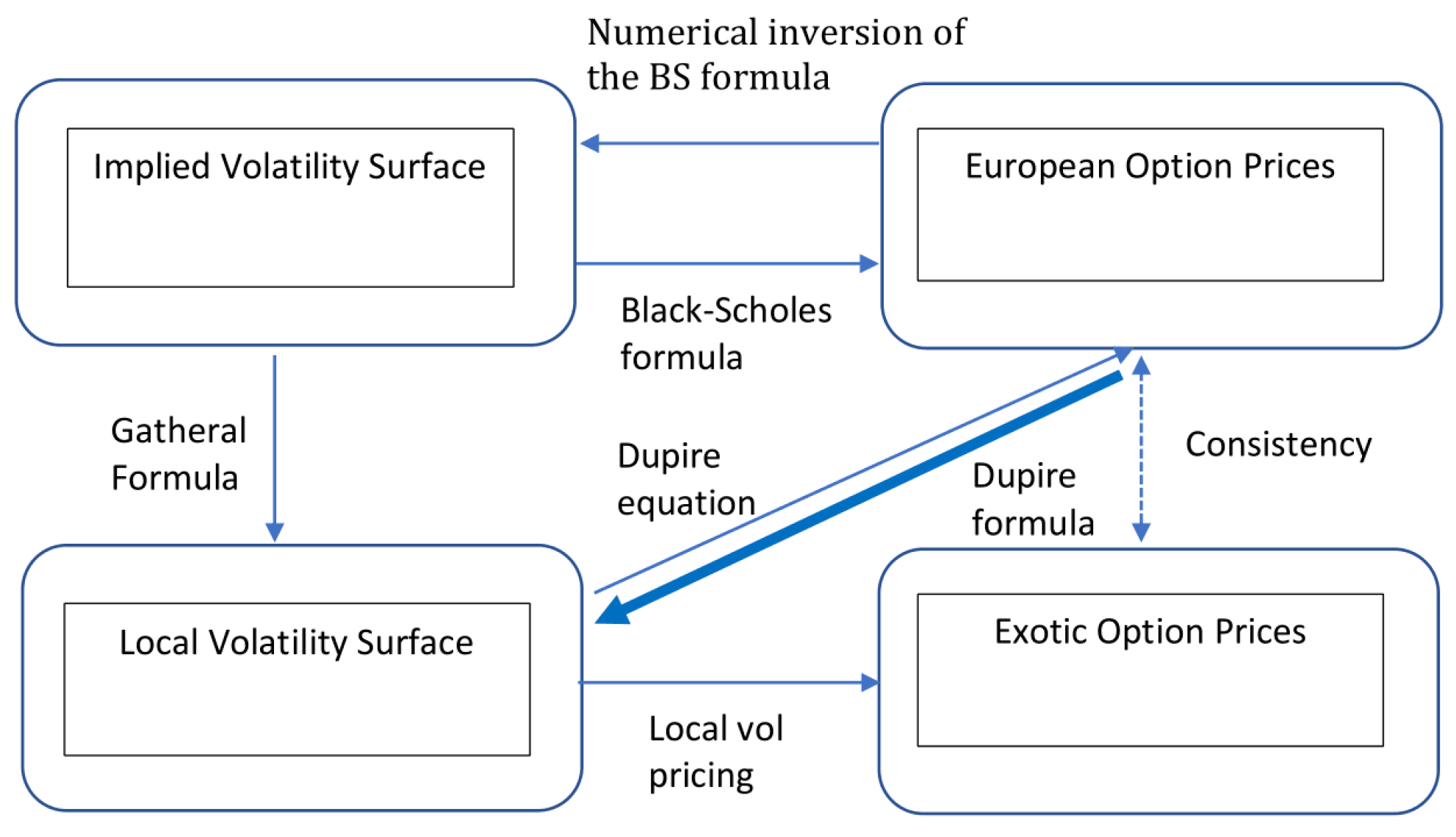
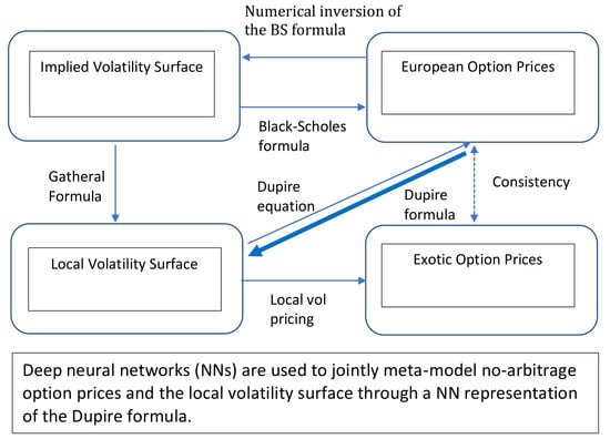
An alternative machine learning approach to local volatility calibration is to use the Gatheral (2011) formula (1.10) to extract the local volatility surface from the Black-Scholes implied volatilities corresponding to the market prices. Figure 1 recasts the two approaches in the general option pricing perspective. The second approach will be considered in a forthcoming paper.

2. Problem Statement

We consider European vanilla option prices on a stock or index S. We assume that a deterministic short interest rate term structure r ( t ) of the corresponding economy has been bootstrapped from the its zero coupon curve, and that a term structure of deterministic continuous-dividend-yields q ( t ) on S has then been extracted from the prices of the forward contracts on S. The assumption of deterministic rates and dividends is for consistency with local volatility models, in the perspective, later in the paper, of numerical experiments on equity options (using Crépey 2002 as a benchmark).
Without restriction given the call-put parity relationship, we only consider put option prices. We denote by P ( T , K ) the market price of the put option with maturity T and strike K on S, observed for a finite number of pairs ( T , K ) at a given day.
Our goal is to construct a nonarbitrable put price surface P : R + × R + R + in C 1 , 2 ( ( 0 , + ) × R + ) C 0 ( R + × R + ) , interpolating P up to some error term. As is well known, the corresponding local volatility surface, say σ ( · , · ) , is given by the Dupire (1994) formula
σ 2 ( T , K ) 2 = T P ( T , K ) + ( r q ) K K P ( T , K ) + q P ( T , K ) K 2 K 2 2 P ( T , K ) .
In terms of p ( T , k ) = exp ( 0 T q ( t ) d t ) P ( T , K ) , where k = K exp ( 0 T ( r ( t ) q ( t ) ) d t ) , the formula reads (see Appendix A for a derivation)
σ 2 ( T , K ) 2 = d u p ( T , k ) : = T p ( T , k ) k 2 k 2 2 p ( T , k ) .
We then learn the modified market prices p = p ( T , k ) . Given a rectangular domain of interest in maturity and strike, we rescale further the inputs, T = ( T m i n ( T ) ) / ( m a x ( T ) m i n ( T ) ) and k = ( k m i n ( k ) ) / ( m a x ( k ) m i n ( k ) , so that the domain of the pricing map is Ω : = [ 0 , 1 ] 2 . This rescaling avoids any one independent variable dominating over another during the fitting. For ease of notation, we shall hereon drop the superscript.
For the Dupire Formula (1) to be meaningful, its output must be nonnegative. This holds, in particular, whenever the interpolating map p exhibits nonnegative derivatives w.r.t. T and second derivative w.r.t. k, i.e.,
T p ( T , k ) 0 , k 2 2 p ( T , k ) 0 .
In both networks considered in the paper, these derivatives are available analytically via the neural network automatic differentiation capability. Hard or soft constraints can be used to enforce these shape properties, exactly in the case of hard constraints and approximately (via regularization) in the case of soft constraints. More generally, see (Roper 2010, Theorem 2.1) for a full and detailed statement of the static non-arbitrage relationships conditions on European vanilla call (easily transposable to put) option prices, also including, in particular, an initial condition at T = 0 given by the option payoffs. This initial payoff condition will also be incorporated to our learning schemes, in a way described in Section 4.2.

3. Shape Preserving Neural Networks

We consider parameterized maps p = p W , b
( T , k ) R + 2 p p W , b ( T , k ) R + ,
given as deep neural networks with two hidden layers. As detailed in Goodfellow et al. (2016), these take the form of a composition of simpler functions:
p W , b ( x ) = f W ( 3 ) , b ( 3 ) ( 3 ) f W ( 2 ) , b ( 2 ) ( 2 ) f W ( 1 ) , b ( 1 ) ( 1 ) ( x ) ,
where
W = ( W ( 1 ) , W ( 2 ) , W ( 3 ) )   and   b = ( b ( 1 ) , b ( 2 ) , b ( 3 ) )
are weight matrices and bias vectors, and the f ( l ) : = ς ( l ) ( W ( l ) x + b ( l ) ) are semi-affine, for nondecreasing activation functions ς ( l ) applied to their (vector-valued) argument componentwise. Any weight matrix W ( ) R m × n can be expressed as an n column W ( ) = [ w 1 ( ) , , w n ( ) ] of m-vectors, for successively chained pairs ( n , m ) of dimensions varying with l = 1 , 2 , 3 , starting from n = 2 , the number of inputs, for l = 1 , and ending up with m = 1 , the number of outputs, for l = 3 .

3.1. Hard Constraints Approach

In the hard constraints case, our network is sparsely connected in the sense that, with x = ( T , k ) as above,
f W ( 1 ) , b ( 1 ) ( 1 ) ( x ) = [ f W ( 1 , T ) , b ( 1 , T ) ( 1 , T ) ( T ) , f W ( 1 , k ) , b ( 1 , k ) ( 1 , k ) ( k ) ] ,
where W ( 1 , T ) , b ( 1 , T ) and W ( 1 , k ) , b ( 1 , k ) correspond to parameters of sub-graphs for each input, and
f ( 1 , T ) ( T ) : = ς ( 1 , T ) ( W ( 1 , T ) T + b ( 1 , T ) ) , f ( 1 , k ) ( k ) : = ς ( 1 , k ) ( W ( 1 , k ) k + b ( 1 , k ) ) .
To impose the shape constraints relevant for put options, it is then enough to restrict ourselves to nonnegative weights, and to convex (and nondecreasing) activation functions, namely
softplus ( x ) : = ln ( 1 + e x ) ,
except for ς ( 1 , T ) , which will be taken as an S-shaped sigmoid ( 1 + e x ) 1 . Imposing non-negative constraints on weights can be achieved in back-propagation using projection functions applied to each weight after each gradient update.
Hence, the network is convex and nondecreasing in k, as a composition (restricted to the k variable) of convex and nondecreasing functions of k. In T, the network is nondecreasing, but not necessarily convex, because the activation function for the maturity subnetwork hidden layer is not required to be convex—in fact, we choose a sigmoid function.
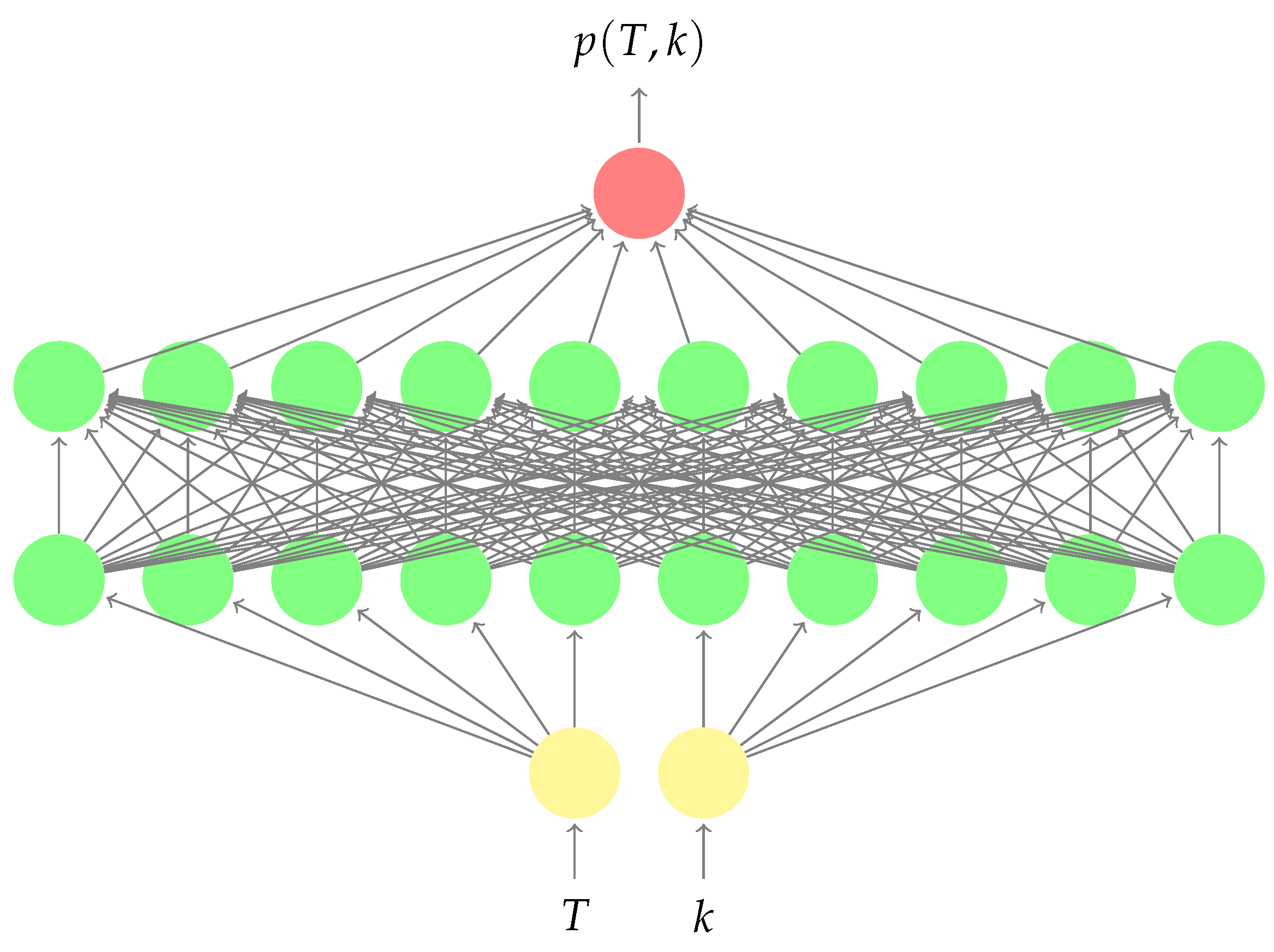
Figure 2 illustrates the shape preserving feed forward architecture with two hidden layers containing 10 hidden nodes. For avoidance of doubt, the figure is not representative of the number of hidden neurons used in our experiments. However, the connectivity is representative. The first input variable, T, is only connected to the first five hidden nodes and the second input variable, k, is only connected to the last five hidden nodes. Effectively, two sub-networks have been created where no information from the input layer crosses the sub-networks until the second hidden layer. In other words, each sub-network is a function of only one input variable. This property is the key to imposing different hard shape constraints w.r.t. each input variable.

3.2. Soft Constraints Approach

However, Theorem 4.1 in Ohn and Kim (2019), which is stated for the reader’s convenience in Appendix B, provides support for our observation, presented in Section 5, that sparsening the network (i.e., splitting) increases the approximation error. Hence, in what follows, we also consider the so called soft constraints approach using a fully connected network, where the static no arbitrage conditions (2) are favored by penalization, as opposed to imposed to hold exactly in the previous hard constraint approach.
Note that only the “hard constraints” approach theoretically guarantees that the associated Dupire formula (1) returns a positive function. While soft constraints reduce the risk of static arbitrage in the sense of mismatch between model and market prices, they do not however fully prevent arbitrages in the sense of violations of the shape conditions (2) in the predicted price surface, especially far from the grid nodes of the training set.
In particular, the penalties only control the corresponding derivatives at the training points. Compliance with the no-arbitrage constraints on the majority of the points in the test set is due only to the regularity of these derivatives. This is not a novel idea. Aubin-Frankowski and Szabo (2020) exploit RKHS regularity to ensure conditions on derivatives in a hard constraint manner with a second order cone optimization. They add a margin to the penalizations so that these derivative conditions are ensured over a targeted neighbourhood of training points. In our case we do not add such a margin to our penalizations. Instead, we add a further half-variance bounds penalization, which both favors even more the shape constraints (without guaranteeing them in theory) and stabilizes the local volatility function calibration, as detailed below.

4. Numerical Methodology

4.1. Training

In general, to fit our fully connected or sparse networks to the available option market prices at a given time, we solve a loss minimization problem of the following form (with λ = 0 in the non-penalized cases), using observations { x i = ( T i , k i ) , p ( x i ) } i = 1 n of n maturity-strike pairs and the corresponding market put prices:
min W , b 1 n i = 1 n | p ( x i ) p ( x i ) | + λ T ϕ ( x i ) .
here p = p W , b , ϕ = ϕ W , b is a regularization penalty vector
ϕ : = [ ( T p ) , ( k 2 2 p ) , ( d u p a ¯ ) + + ( d u p a ̲ ) ] ,
and d u p is related to p through (1). The choice to measure the error p p under the L 1 norm, rather than L 2 norm, in (3) is motivated by a need to avoid allocating too much weight to the deepest in-the-money options. Note that Ackerer et al. (2019) consider a combination of L 1 and L 2 norms. In a separate experiment, not reported here, we additionally investigated using the market convention of vega weighted option prices, albeit to no effect beyond simply using L 1 regularization.
The loss function is non-convex, possessing many local minima and it is generally difficult to find a global minimum. The first two elements in the penalty vector favor the shape conditions (2) and the third element favors lower and upper bounds a ̲ and a ¯ on the estimated half-variance, d u p , where constants (which could also be functions of time) 0 < a ̲ < a ¯ respectively denote desired lower and upper bounds on the surface (at each point in time). Of course, as soon as penalizations are effectively used (i.e., for λ 0 ), a further difficulty, typically involving grid search, is the need to determine suitable values of the corresponding “Lagrange multipliers”
λ = ( λ 1 , λ 2 , λ 3 ) R + 3 ,
ensuring the right balance between fit to the market prices and the targeted constraints.

4.2. Experimental Design

As a benchmark, reference method for assessing the performance of our neural network approaches, we use the Tikhonov regularization approach surveyed Section 9.1 of Crépey (2013), i.e., nonlinear least square minimization of the squared distance to market prices plus a penalisation proportional to the H 1 squared norm of the local volatility function over the (time, space) surface (or, equivalently, to the L 2 norm of the gradient of the local volatility). Our motivation for this choice as a benchmark is, first, the theoretical, mathematical justification for this method provided by Theorems 6.2 and 6.3 in Crépey (2003). Second, it is price (as opposed to implied volatility) based, which makes it at par with our focus on price based neural network local volatility calibration schemes in this paper. Third, it is non parametric (’model free’ in this sense), like our neural network schemes again, and as opposed to various parameterizations such as SABR or SSVI that are used as standard in various segments of the industry, but come without theoretical justification for robustness, are restricted to specific industry segments on which they play the role of a market consensus, and are all implied volatility based. Fourth, an efficient numerical implementation of the Tikhonov method (as we call it for brevity hereafter), already put to the test of hundreds of real datasets in the context of Crépey (2004), is available through Crépey (2002). Fifth, this method is itself benchmarked to other (spline interpolation and constrained stochastic control) approaches Section 7 of Crépey (2002).
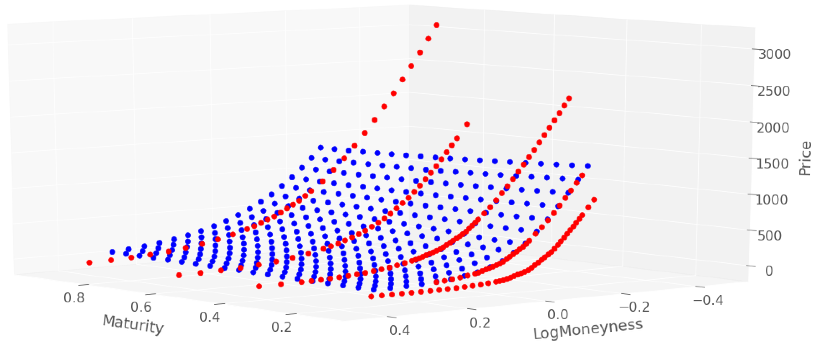
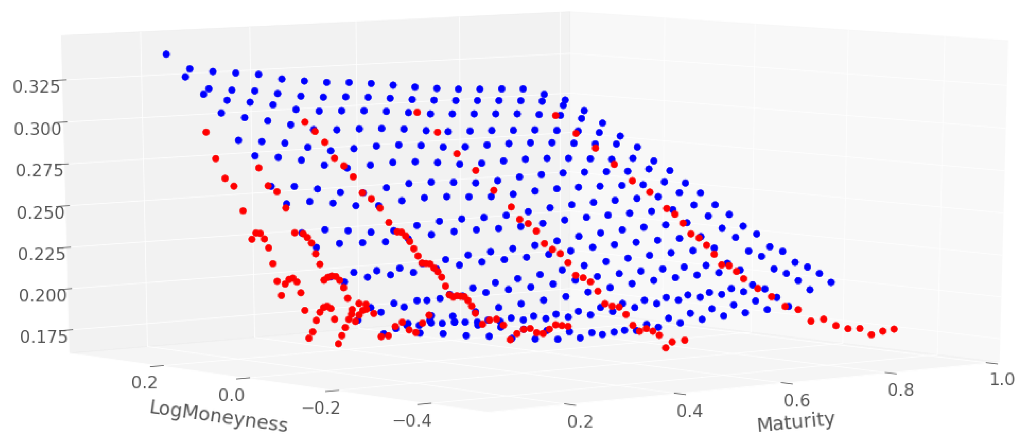
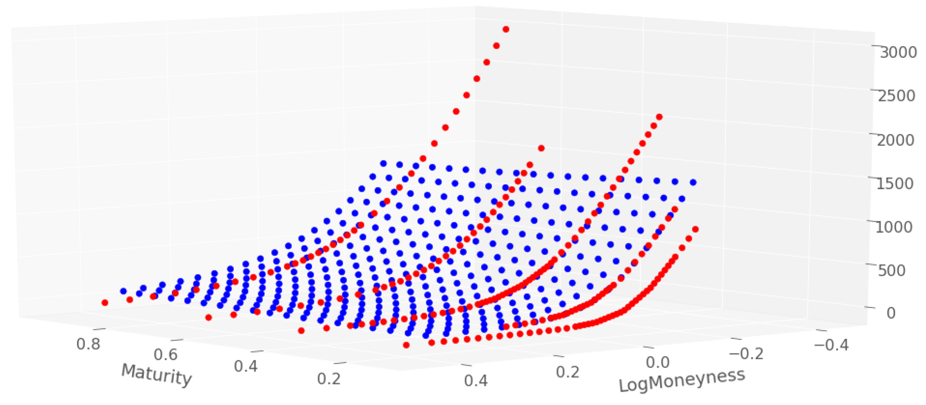
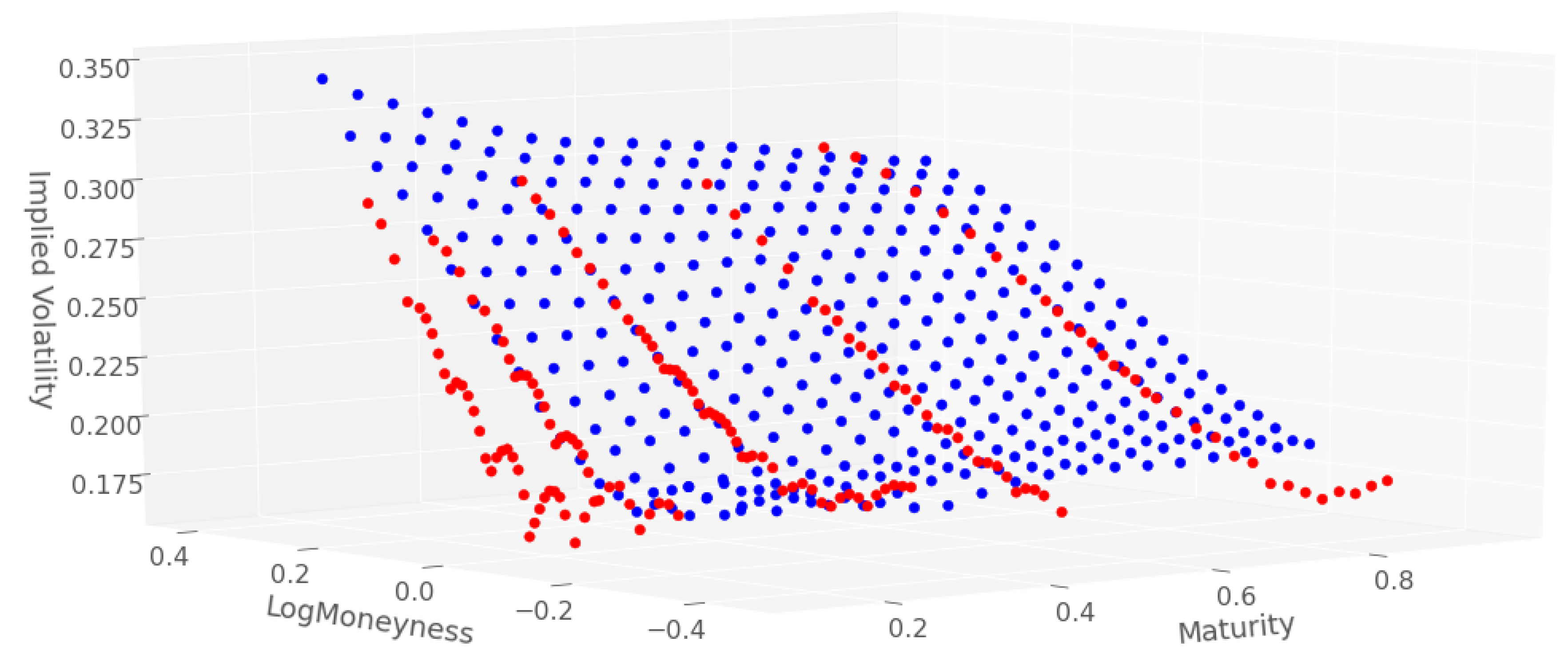
Our training sets were prepared using daily datasets of DAX index European vanilla options of different available strikes and maturities, listed on the 7th, 8th (by default below), and 9th, August 2001, i.e., same datasets as already used in previous work Crépey (2002, 2004), for benchmarking purposes. The corresponding values of the underlying were S = 5752.51 , 5614.51 and 5512.28 . The associated interest rate and dividend yield curves were constructed from zero-coupon and forward curves, themselves obtained from quotations of standard fixed income linear instruments and from call/put parity applied to the option market prices. Each training set was composed of about 200 option market prices plus the put payoffs for all strikes present in the training grid. For each day of data (see e.g., Figure 3 and Figure 4), a test set of about 350 points was generated by computing, thanks to a trinomial tree, option prices for a regular grid of strikes and maturities, in the local volatility model calibrated to the corresponding training set by the benchmark Tikhonov calibration method of Crépey (2002).
Each network had two hidden layers, each with 200 neurons per hidden layer. Note that Dugas et al. (2009) only used one hidden layer. Using two was found important in practice in our case. All networks were fitted with an ADAM optimizer. In order to achieve the convergence of the training procedure toward a local minimum of the loss criterion, the learning rate was divided by 10 whenever no improvement in the error on the training set was observed during 100 consecutive epochs. The total number of epochs was limited to 10,000 because of the limited number of market prices. Thus we opted for a batch learning with numerous epochs.
After training, a local volatility surface was extracted from the interpolated prices by application of the Dupire Formula (1), leveraging on the availability of the corresponding exact sensitivities, i.e., using automatic algorithmic differentiation (AAD) and not finite differences. This local volatility surface was then compared with the one obtained in Crépey (2002).
Moreover, we assessed numerically four different combinations of network architectures and optimization criteria, i.e.,
  • sparse (i.e., split) network and hard constraints, so λ 1 = λ 2 = 0 in (3) and (4),
  • sparse network but soft constraints, i.e., ignoring the non-negative weight restriction in Section 3.1, but using λ 1 , λ 2 > 0 in (3) and (4),
  • dense network and soft constraints, i.e., for λ 1 , λ 2 > 0 in (3) and (4),
  • dense network and no shape constraints, i.e., λ 1 = λ 2 = 0 in (3) and (4).
Moreover, these four configurations were tried both without (Section 5) and with (Section 6) half-variance bounds penalization, i.e., for λ 3 = 0 vs. λ 3 > 0 in (3) and (4), cases referred to hereafter as without/with Dupire penalization.
In each case the error between the prices of the calibrated model and the market data were evaluated on both the training and an out-of-sample test set. Unless reported otherwise, all numerical results shown below correspond to test sets.
All our numerical experiments were run under Google Colab with 13 GB of RAM and a dual core CPU of 2.2 GHz.

5. Numerical Results without Dupire Penalization

Table 1 shows the pricing RMSEs for four different combinations of architecture and optimization criteria without half-variance bounds, i.e., for λ 3 = 0 (3) and (4). For the sparse network with hard constraints, we thus have λ = 0 . For the sparse and dense networks with soft constraints (i.e., penalization but without the conditions on the weights of Section 3), we set λ = [ 1.0 × 10 5 , 1.0 × 10 3 , 0 ] .
The sparse network with hard constraints is observed to exhibit significant pricing error, which suggests that this approach is too limited in practice to approach market prices. This conclusion is consistent with Ackerer et al. (2019), who choose a soft-constraints approach in the implied volatility approximation (in contrast to our approach which approximates prices).
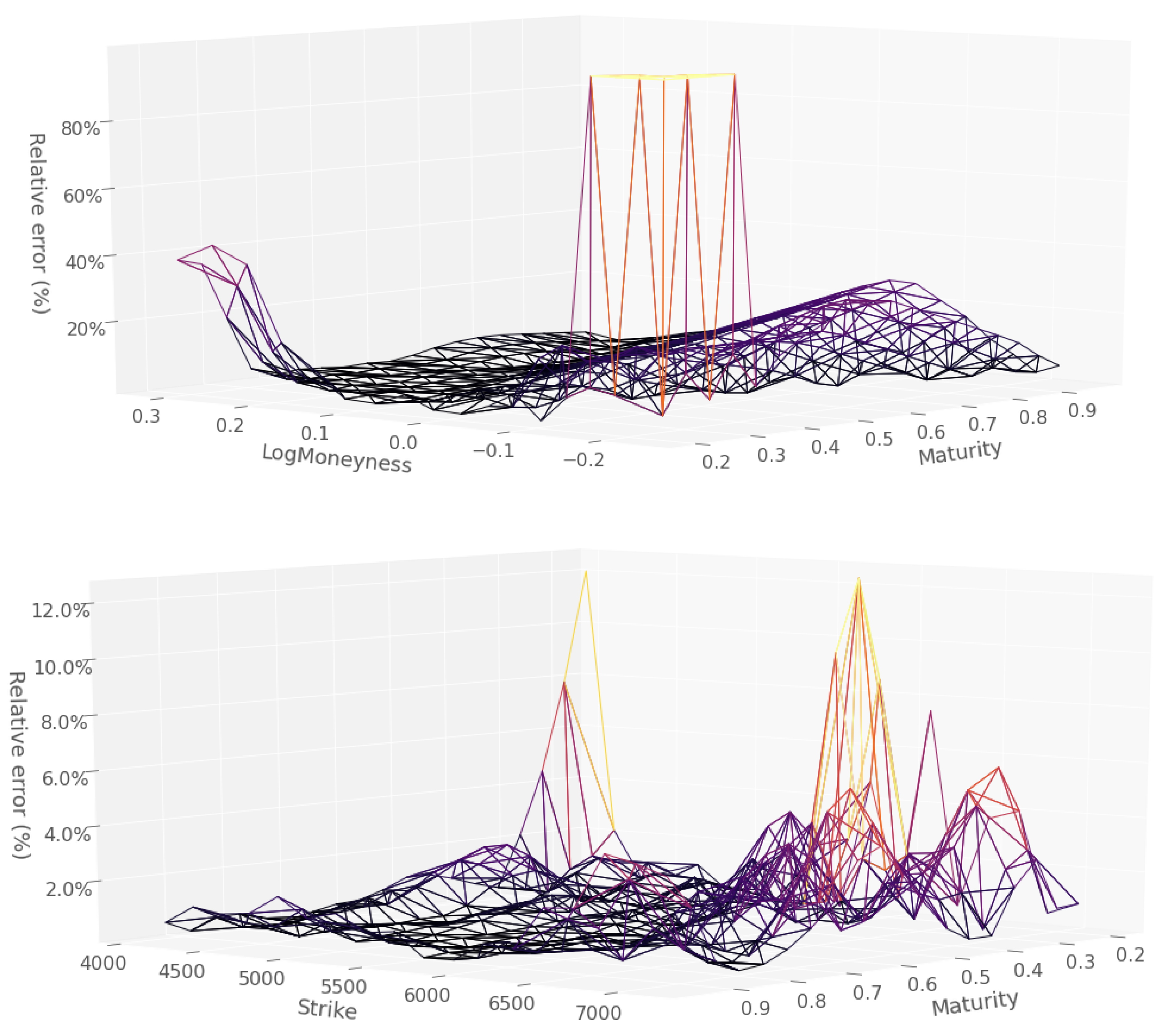
Figure 5 compares the percentage errors in implied volatilities using the sparse network with hard constraints and the dense network with soft constraints approaches, corresponding to the columns 1 and 3 of Table 1. Relative errors with hard constraints exceeded 10% on most the training grid oppositely to dense network with soft constraints. This confirms that the error levels of the hard constraints approach were too high to imagine a practical use of this approach: the corresponding model would be immediately arbitrable in relation to the market. Those of the soft constraint approach were much more acceptable, with high errors confined to short maturities or far from the money, i.e., in the region where prices provide little information on volatility.
Table 2 shows the fraction of points in the neural network price surface which violate the static arbitrage conditions. The table compares the same four methods listed in Table 3 applied to training and testing sets. We recall that, in theory, only the sparse network with hard constraints guarantees zero arbitrages. However, we observe that the inclusion of soft constraints reduced the number of arbitrage constraints on the training set when compared with no constraints. The trend was less pronounced for the test set. However, in the absence of hard constraints, the effect of adding soft constraints was always preferable than excluding them entirely.

6. Numerical Results with Dupire Penalization

We now introduce half-variance bounds into the penalization to improve the overall fit in prices and stabilize the local volatility surface. Table 3 shows the RMSEs in absolute pricing resulting from repeating the same set of experiments reported in Table 1, but with the half-variance bounds included in the penalization. For the sparse network with hard constraints, we set λ = [ 0 , 0 , 10 ] and choose a ̲ = 0.05 2 / 2 and a ¯ = 0.4 2 / 2 . For the sparse and dense networks with soft constraints, we set λ = [ 1.0 × 10 5 , 1.0 × 10 3 , 10 ] . Compared to Table 1, we observed improvement in the test error for the hard and soft constraints approaches when including the additional local volatility penalty term. Table 4 is the analog of Table 2, with similar conclusions. Note that, here as above, the arbitrage opportunities that arose were not only very few (except in the unconstrained case), but also very far from the money and, in fact, mainly regarded the learning of the payoff function, corresponding to the horizon T = 0 . See for instance Figure 6 for the location of the violations that arose in the unconstrained case with Dupire penalization. Hence such apparent ‘arbitrage opportunities’ could not necessarily be monetized once liquidity was accounted for.
Figure 7 is the analog of Figure 3, with test (i.e., Tikhonov trinomial tree) prices in blue replaced by the prices predicted by the dense network with soft constraints and Dupire penalization. The (blue) prices predicted by the neural network in Figure 7, and the corresponding implied volatilities in Figure 8, did not exhibit any visible inter-extrapolation pathologies, they were in fact visually indistinguishable from the respective (blue) testing prices and implied volatilities of Figure 3 and Figure 4.
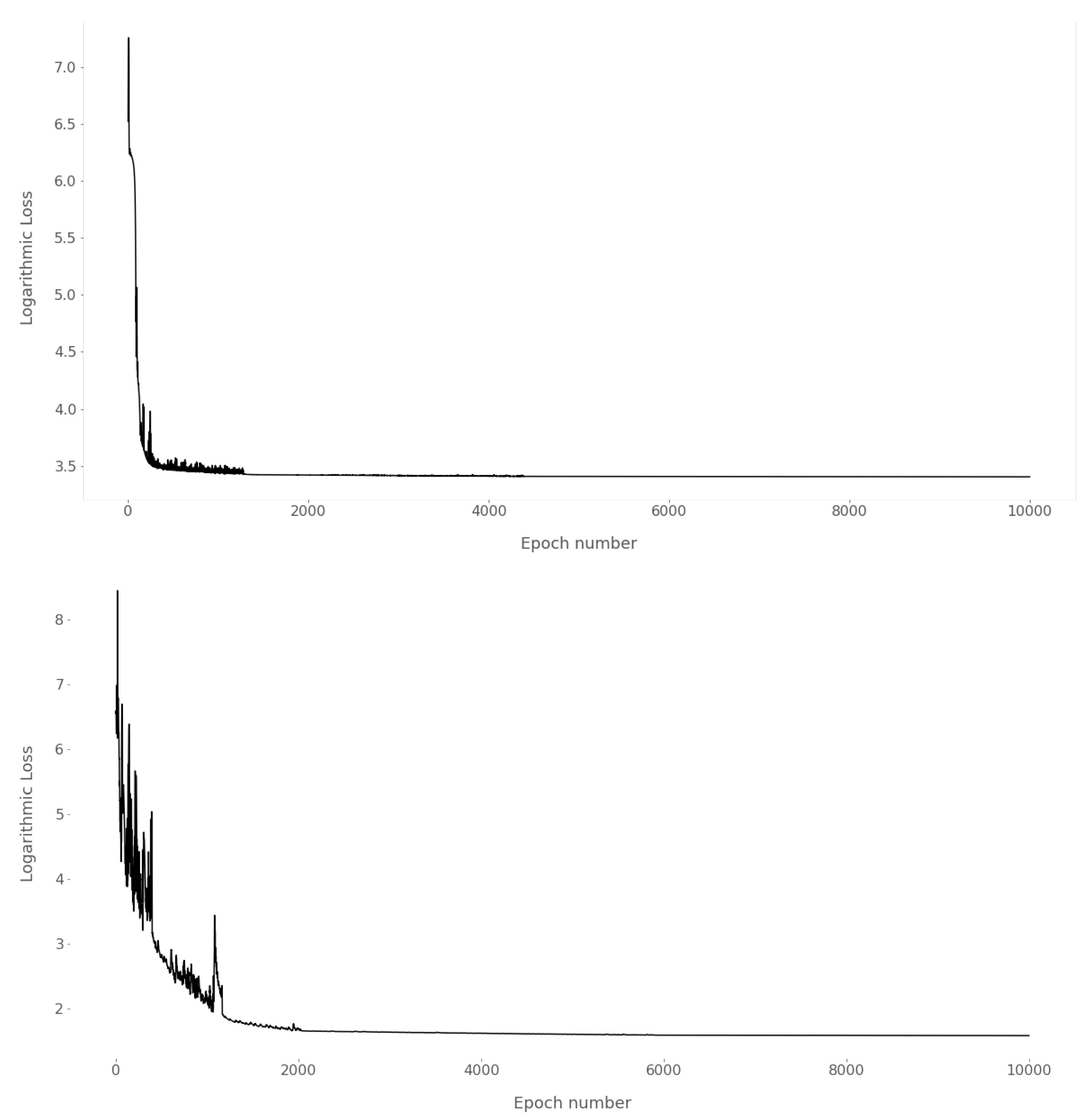
For completeness, we additionally provide further diagnostic results. Figure 9 shows the convergence of the loss function against the number of epochs using either hard constraints or soft constraints. The spikes triggered decays of the learning rates so that the training procedure could converge toward a local minimum of the loss criterion (cf. Section 4.2). We observed that the loss function converged to a much smaller value using a dense network with soft constraints and that either approach converged in at most 2000 epochs.
Table 5 provides some further insight into the effect of architectural parameters, although it is not intended to be an exhaustive study. Here, only the number of units in the hidden layers was varied, while keeping all other parameters except the learning rate fixed, to study the effect on error in the price and implied volatility surfaces. The price RMSE for the testing set primarily provided justification for the choice of 200 hidden units per layer: the RMSE was 3.55. We further observed the effect of reduced pricing error on the implied volatility surface: 0.0036 was the lowest RMSE of the implied volatility test surface across all parameter values.
Table 6 shows the pricing RMSEs resulting from the application of different stochastic gradient descent algorithms under the soft constraints approach with dense network and Dupire penalization. ADAM (our choice everywhere else in the paper, cf. the next-to-last column in Table 3) and root mean square propagation (RMSProp, another well known SGD procedure) exhibited a comparable performance. A Nesterov accelerated gradient procedure, with momentum parameter set to 0.9 as standard, obtained much less favorable results. As opposed to ADAM and RMSProp, Nesterov accelerated momentum did not reduce the learning rate during the optimization.

7. Robustness

In this concluding section of the paper, we assess the robustness of the different approaches in terms of, first, the numerical stability of the local volatility function recalibrated across successive calendar days, and second, of a Monte Carlo backtesting repricing error.

7.1. Numerical Stability through Recalibration

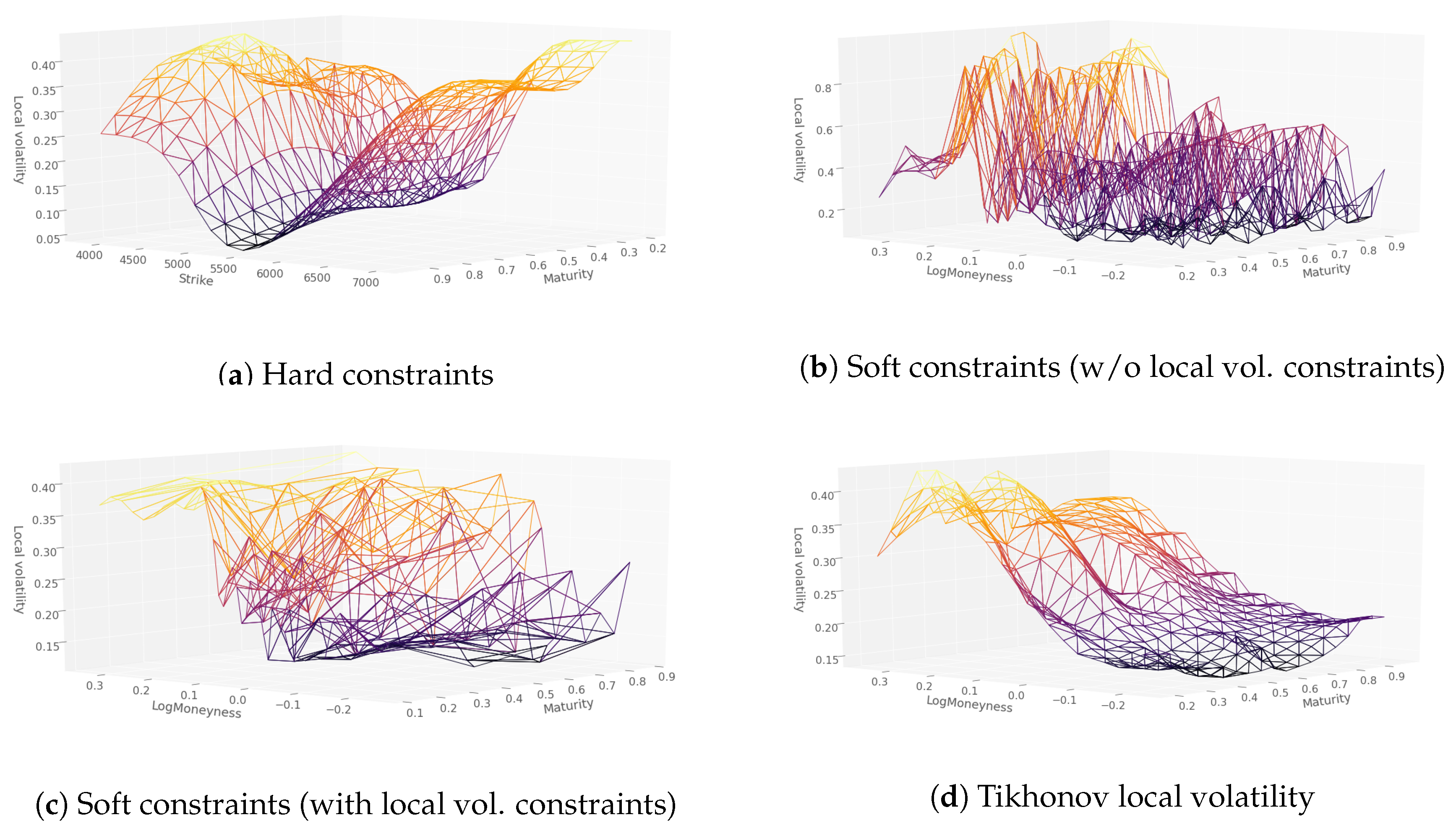
Figure 10, Figure 11 and Figure 12 show the comparison of the local volatility surfaces obtained using hard constraints (sparse network) without Dupire penalization, dense network and soft constraints without and with Dupire penalization, as well as the Tikhonov regularization approach of Crépey (2002), on price quotes listed on August 7th, 8th, and 9th, 2001, respectively. The soft constraint approach without Dupire penalization is both irregular (exhibiting outliers on a given day) and unstable (from day to day). In contrast, the soft constraint approach with Dupire penalization yields a more regular (at least, less spiky) local volatility surface, both at fixed calendar time and in terms of stability across calendar time. From this point of view the results are then qualitatively comparable to those obtained by Tikhonov regularization (which is however quicker, taking of the order of 30 s to run).

7.2. Monte Carlo Backtesting Repricing Error

Finally, we evaluate the performance of the models in a backtesting Monte Carlo exercise. Namely, the options in each testing grid are repriced by Monte Carlo with 10 5 paths of 100 time steps in the model
d S t S t = r ( t ) q ( t ) d t + σ ( t , S t ) d W t ,
using differently calibrated local volatility functions σ ( · , · ) in (5), for each of the 7th, 8th, and 9th August dataset. Table 7 shows the corresponding Monte Carlo backtesting repricing errors, using the option market prices from the training grids as reference values in the corresponding RMSEs. The neural network approaches provide a full surface of prices and local volatilities, as opposed to values at the calibration trinomial tree nodes only in the case of Tikhonov, for which the Monte Carlo backtesting exercise thus requires an additional layer of local volatility inter-extrapolation, here achieved by a nearest neighbors algorithm. We see from the table that both the benchmark Tikhonov method and the dense network soft constraints approach with Dupire penalization yield very reasonable and acceptable repricing errors (with still a certain advantage to the Tikhonov method), unlike the hard constraints approaches. Moreover, the Dupire penalization is essential for extracting a decent local volatility function: The dense network with soft constraint but without this penalization yields very poor Monte Carlo repricing RMSEs.
The residual gap between the Monte Carlo RMSEs of the (even best) neural network local volatility and of the Tikhonov local volatility can seem disappointing. However we should keep in mind that the neural network can evaluate quickly a local volatility on any node outside the training grid, whereas Tikhonov then requires a further layer of interpolation (or a new calibration). Furthermore, any vanilla option price can be accurately and quickly obtained by neural prediction (better than by Monte Carlo repricing as above). Table 8 shows training set RMSEs of thus predicted prices against markets prices equivalent to (in fact, slightly better than) RMSEs of Tikhonov trinomial tree prices against the same markets prices. These are of course only in-sample errors, but the additional findings of Table 7 suggest that these good results are not just overfitting.

8. Conclusions

We introduced three variations of deep learning methodology to enforce no-arbitrage interpolation of European vanilla put option prices: (i) modification of the network architecture to embed shape conditions (hard constraints), (ii) use of shape penalization to favor these conditions (soft constraints), and (iii) additional use of local half-variance bounds in the penalization via the Dupire formula.
Our experimental results confirm that hard constraints, although providing the only fail-safe approach to no-arbitrage approximation, reduce too much the representational power of the network numerically. Soft constraints provide much more accurate prices and implied volatilities, while only leaving space for sporadic arbitrage opportunities, which are not only occasional but also very far from the money, hence do not necessarily correspond to monetizable arbitrage opportunities once liquidity is accounted for. Once the Dupire formula is included in the penalization, the corresponding local volatility surface is also reasonably regular, at fixed day, and stable, in terms of both out-of-sample performance at fixed day and dynamically from day to day. The performance of the neural network local volatility calibration method then gets close to the one of the classical Tikhonov regularization method of Crépey (2002), but not better. It is also slower. However, the neural network provides the full surface of prices and local volatilities, as opposed to values at the nodes of a trinomial tree only under the approach of Crépey (2002).
We thus enrich the machine learning literature on neural networks metamodeling of vanilla option prices in three respects: first, by considering the associated local volatility, which is interesting both in itself and as a tool for improving the learning of the option prices in the first place; second, by working with real data; third, by systematically benchmarking our results with the help of a proven (both mathematically and numerically) classical, non machine learning calibration procedure, i.e., Tikhonov regularization. In this article, we focused on machine learning schemes for extracting the local volatility from option prices. The use of option implied volatilities will be considered in a further paper.

Author Contributions

Authors M.C., S.C., M.D. contributed equally to each section of this paper. All authors have read and agreed to the published version of the manuscript.

Funding

This research received no external funding.

Conflicts of Interest

The authors declare no conflict of interest.

Appendix A. Change of Variables in the Dupire Equation

Letting g ( T , K ) = P ( T , K ) exp 0 T q d t , note that
K P ( T , K ) = exp 0 T q d t K g ( T , K ) , K 2 2 P ( T , K ) = exp 0 T q d t K 2 2 g ( T , K ) T P ( T , K ) = exp 0 T q d t T g ( T , K ) q g ( T , K ) .
The Dupire formula is then rewritten in terms of g as
T g ( T , K ) = 1 2 σ 2 ( T , K ) K 2 K 2 2 g ( T , K ) ( r q ) K K g ( T , K ) .
Through the additional change of variables p ( T , k ) = g ( T , K ) , where k = exp 0 T ( r q ) d t K , we obtain
K g ( T , K ) = K p ( T , k ) = k p ( T , k ) K k = exp 0 T ( r q ) d t k p ( T , k ) K 2 2 g ( T , K ) = K 2 2 p ( T , k ) = k K p ( T , k ) K k = exp 2 0 T ( r q ) d t k 2 2 p ( T , k ) T g ( T , K ) = T p ( T , k ) + T k k p ( T , k ) = T p ( T , k ) ( r q ) k k p ( T , k )
and arrive at the modified Dupire equation:
T p ( T , k ) = 1 2 σ 2 ( T , K ) k 2 k 2 2 p ( T , k )
conveniently written as the Dupire half-variance Formula (1).

Appendix B. Network Sparsity and Approximation Error Bound

We recall a result from Ohn and Kim (2019) which describes how the sparsity in a neural network affects its approximation error.
Let us denote the network parameters θ : = ( W , b ) . We define the network parameter space in terms of the layers width L and depth N, and numbers of inputs and outputs,
Θ i , o ( L , N ) : = { θ : L ( θ ) L , n m a x ( θ ) N , i n ( θ ) = i , o u t ( θ ) = o } .
We also define the restricted parameter space
Θ i , o ( L , N , Σ , B ) : = { θ Θ i , o ( L , N ) : | θ | 0 Σ , | θ | B } ,
where | θ | 0 is the number of nonzero components in θ and | θ | is the largest absolute value of elements of θ . Let the activation ς be either piecewise continuous or locally quadratic2. For example, softplus and sigmoid functions are locally quadratic. Let the function being approximated, p H α , R ( [ 0 , 1 ] i ) be Hölder smooth with parameters α > 0 and R > 0 , where H α , R ( Ω ) : = { p H α ( Ω ) : | | p | | H α ( Ω ) R } . Then Theorem 4.1 in Ohn and Kim (2019) states the existence of positive constants L 0 , N 0 , Σ 0 , B 0 depending only on i , α , R and ς s.t. for any ϵ > 0 , the neural network
θ ϵ Θ i , 1 L 0 l o g ( 1 / ϵ ) , N 0 ϵ i / α , Σ 0 ϵ i / α l o g ( 1 / ϵ ) , B 0 ϵ 4 ( i / α + 1 )
satisfies sup x [ 0 , 1 ] i | p ( x ) p θ ϵ ( x ) | ϵ . Figure A1 shows the upper bound Σ on the network sparsity, | θ | 0 Σ , as a function of the error tolerance ϵ and Hölder smoothness, α , of the function being approximated. Keeping the number of neurons in each layer fixed, the graph shows that a denser network, with a higher upper bound, results in a lower approximation error. Conversely, networks with a low number of non-zero parameters, due to zero weight edges, exhibit larger approximation error. In the context of no-arbitrage pricing, the theorem suggests a tradeoff between using a sparse network to enforce the shape constraints, yet increasing the approximation error. The adverse effect of using a sparse network should also diminish with increasing smoothness in the function being approximated.
Figure A1. The upper bound on the network sparsity, | θ | 0 Σ , as a function of the error tolerance ϵ and Hölder smoothness, α , of the function being approximated. As ϵ or α decrease, the value of Σ is observed to increase. The plot is shown for i = 2 and Σ 0 = 10 .
Risks 08 00082 g0a1

References

  1. Ackerer, Damien, Natasa Tagasovska, and Thibault Vatter. 2019. Deep Smoothing of the Implied Volatility Surface. Available online: https://ssrn.com/abstract=3402942 (accessed on 29 July 2020).
  2. Aubin-Frankowski, Pierre-Cyril, and Zoltan Szabo. 2020. Hard shape-constrained kernel machines. arXiv arXiv:2005.12636. [Google Scholar]
  3. Crépey, Stéphane. 2002. Calibration of the local volatility in a trinomial tree using Tikhonov regularization. Inverse Problems 19: 91. [Google Scholar] [CrossRef] [Green Version]
  4. Crépey, Stéphane. 2003. Calibration of the local volatility in a generalized Black–Scholes model using Tikhonov regularization. SIAM Journal on Mathematical Analysis 34: 1183–206. [Google Scholar] [CrossRef] [Green Version]
  5. Crépey, Stéphane. 2004. Delta-hedging vega risk? Quantitative Finance 4: 559–79. [Google Scholar] [CrossRef]
  6. Crépey, Stéphane. 2013. Financial Modeling: A Backward Stochastic Differential Equations Perspective. Springer Finance Textbooks. Berlin: Springer. [Google Scholar]
  7. Dugas, Charles, Yoshua Bengio, François Bélisle, Claude Nadeau, and René Garcia. 2009. Incorporating functional knowledge in neural networks. Journal of Machine Learning Research 10: 1239–62. [Google Scholar]
  8. Dupire, Bruno. 1994. Pricing with a smile. Risk 7: 18–20. [Google Scholar]
  9. Garcia, René, and Ramazan Gençay. 2000. Pricing and hedging derivative securities with neural networks and a homogeneity hint. Journal of Econometrics 94: 93–115. [Google Scholar] [CrossRef] [Green Version]
  10. Gatheral, Jim. 2011. The Volatility Surface: A Practitioner’s Guide. Hoboken: Wiley. [Google Scholar]
  11. Gençay, Ramazan, and Min Qi. 2001. Pricing and hedging derivative securities with neural networks: Bayesian regularization, early stopping, and bagging. IEEE Transactions on Neural Networks 12: 726–34. [Google Scholar] [CrossRef] [PubMed]
  12. Goodfellow, Ian, Yoshua Bengio, and Aaron Courville. 2016. Deep Learning. Cambridge: MIT Press. [Google Scholar]
  13. Hutchinson, James M., Andrew W. Lo, and Tomaso Poggio. 1994. A nonparametric approach to pricing and hedging derivative securities via learning networks. The Journal of Finance 49: 851–89. [Google Scholar] [CrossRef]
  14. Itkin, A. 2019. Deep learning calibration of option pricing models: Some pitfalls and solutions. arXiv arXiv:1906.03507. [Google Scholar]
  15. Márquez-Neila, Pablo, Mathieu Salzmann, and Pascal Fua. 2017. Imposing hard constraints on deep networks: Promises and limitations. arXiv arXiv:1706.02025. [Google Scholar]
  16. Ohn, Ilsang, and Yongdai Kim. 2019. Smooth Function Approximation by Deep Neural Networks with General Activation Functions. Entropy 21: 627. [Google Scholar] [CrossRef] [Green Version]
  17. Roper, Michael. 2010. Arbitrage Free Implied Volatility Surfaces. Available online: https://talus.maths.usyd.edu.au/u/pubs/publist/preprints/2010/roper-9.pdf (accessed on 29 July 2020).
1
The call and put prices must also be decreasing and increasing by strike respectively.
2
A function ς : R R is locally quadratic if ∃ an open interval ( a , b ) R over which ς is three times continuously differentiable with bounded derivatives and t ( a , b ) s.t. ς ( t ) 0 and ς ( t ) 0 .
Figure 1. Mathematical connections between option prices, implied, and local volatility, and the goal of this paper, namely to use the Dupire formula with deep neural networks to jointly approximate the vanilla price and local volatility surfaces.
Risks 08 00082 g001
Figure 2. A shape preserving (sparse) feed forward architecture with one hidden layer containing 10 hidden nodes. The first input variable, T, is only connected to the five left most hidden nodes and the second input variable, k, is only connected to the five right most hidden nodes.
Risks 08 00082 g002
Figure 3. DAX put prices from training grid (red points) and testing grid (blue points), 8 August 2001.
Risks 08 00082 g003
Figure 4. Same as Figure 3 in implied volatility scale.
Risks 08 00082 g004
Figure 5. Percentage relative error in the implied volatilities using (top) hard constraints (bottom) dense networks with soft constraints.
Risks 08 00082 g005

Figure 6. Location of the violations, denoted by black crosses, corresponding to the right column in Table 4.
Risks 08 00082 g006

Figure 7. Put prices from training grid (red points) and NN predicted prices at testing grid nodes (blue points), DAX 8 August 2001.
Risks 08 00082 g007

Figure 8. Same as Figure 7 in implied volatility scale.
Risks 08 00082 g008

Figure 9. Logarithmic RMSE through epochs (top) hard constraints (bottom) dense networks with soft constraints.
Risks 08 00082 g009

Figure 10. Local volatility for 7 August 2001.
Risks 08 00082 g010
Figure 11. Local volatility for 8 August 2001.
Risks 08 00082 g011
Figure 12. Local volatility for 9 August 2001.
Risks 08 00082 g012
Table 1. Pricing RMSE (absolute pricing errors) and training times without Dupire penalization.
Sparse NetworkDense Network
Hard ConstraintsSoft ConstraintsSoft ConstraintsNo Constraints
Training dataset28.136.872.282.56
Testing dataset28.914.093.533.77
Indicative training times200 s400 s200 s120 s
Table 2. The fraction of static arbitrage violations without Dupire penalization.
Sparse NetworkDense Network
Hard ConstraintsSoft ConstraintsSoft ConstraintsNo Constraints
Training dataset01/254063/254
Testing dataset02/360044/360
Table 3. Price RMSE (absolute pricing errors) and training times with Dupire penalization.
Sparse NetworkDense Network
Hard ConstraintsSoft ConstraintsSoft ConstraintsNo Constraints
Training dataset28.043.442.483.48
Testing dataset27.073.333.364.31
Indicative training times400 s600 s300 s250 s
Table 4. The fraction of static arbitrage violations with Dupire penalization.
Sparse NetworkDense Network
Hard ConstraintsSoft ConstraintsSoft ConstraintsNo Constraints
Training dataset00030/254
Testing dataset02/36005/360
Table 5. Sensitivity of the errors to the number of hidden units. Note that these results are generated using the dense network with soft constraints and Dupire penalization.
# Hidden UnitsSurfaceRMSE
TrainingTesting
50Price3.013.60
Impl. Vol.0.01730.0046
100Price3.143.66
Impl. Vol.0.03040.0049
200Price2.733.55
Impl. Vol.0.01810.0036
300Price2.843.88
Impl. Vol.0.01800.0050
400Price2.883.56
Impl. Vol.0.06600.0798
Table 6. Pricing RMSEs corresponding to different stochastic gradient descents (soft constraints approach with dense network and Dupire penalization).
Train RMSETest RMSE
ADAM2.483.36
Nesterov accelerated gradient5.676.92
RMSProp2.763.66
Table 7. Monte Carlo backtesting repricing RMSEs on training grid against market prices.
σ ( · , · ) Tikhonov
Monte Carlo
Dense Network
with Soft Constraints
and Dup. penal.
Dense Network
with Soft Constraints
Hard Constraint
with Dup. Penal.
Hard Constraint
w/o Dup. Pen.
7 August 20015.4210.1868.4848.5750.44
8 August 20015.557.4450.8256.6356.98
9 August 20014.608.1859.3966.2365.50
Table 8. Training set RMSEs of Tikhonov trinomial tree vs. NN predicted prices against market prices.
σ ( · , · ) Tikhonov Trin. TreeNN Pred. (Dense Network with
Soft Constraints and Dup. Penal).
7 August 20012.422.66
8 August 20012.672.48
9 August 20012.452.34