Article

A Generative Adversarial Network Approach to Calibration of Local Stochastic Volatility Models

1
Department of Statistics and Operations Research, Data Science @ Uni Vienna, University of Vienna, Oskar-Morgenstern-Platz 1, 1090 Wien, Austria
2
ETH Zürich, D-MATH, Rämistrasse 101, CH-8092 Zürich, Switzerland
*
Author to whom correspondence should be addressed.
Risks 2020, 8(4), 101; https://doi.org/10.3390/risks8040101
Submission received: 9 June 2020 / Revised: 17 September 2020 / Accepted: 18 September 2020 / Published: 27 September 2020
(This article belongs to the Special Issue Machine Learning in Finance, Insurance and Risk Management)

Abstract

:
We propose a fully data-driven approach to calibrate local stochastic volatility (LSV) models, circumventing in particular the ad hoc interpolation of the volatility surface. To achieve this, we parametrize the leverage function by a family of feed-forward neural networks and learn their parameters directly from the available market option prices. This should be seen in the context of neural SDEs and (causal) generative adversarial networks: we generate volatility surfaces by specific neural SDEs, whose quality is assessed by quantifying, possibly in an adversarial manner, distances to market prices. The minimization of the calibration functional relies strongly on a variance reduction technique based on hedging and deep hedging, which is interesting in its own right: it allows the calculation of model prices and model implied volatilities in an accurate way using only small sets of sample paths. For numerical illustration we implement a SABR-type LSV model and conduct a thorough statistical performance analysis on many samples of implied volatility smiles, showing the accuracy and stability of the method.

Graphical Abstract

1. Introduction

Each day a crucial task is performed in financial institutions all over the world: the calibration of stochastic models to current market or historical data. So far the model choice was not only driven by the capacity of capturing empirically observed market features well, but also by the computational tractability of the calibration process. This is now undergoing a big change since machine-learning technologies offer new perspectives on model calibration.
Calibration is the choice of one model from a pool of models, given current market and historical data. Depending on the nature of data this is considered to be an inverse problem or a problem of statistical inference. We consider here current market data, in particular volatility surfaces, therefore we rather emphasize the inverse problem point of view. We however stress that it is the ultimate goal of calibration to include both data sources simultaneously. In this respect machine learning might help considerably.
We can distinguish three kinds of machine learning-inspired approaches for calibration to current market prices: First, having solved the inverse problem already several times, one can learn from this experience (i.e., training data) the calibration map from market data to model parameters directly. Let us here mention one of the pioneering papers by Hernandez (2017) that applied neural networks to learn this calibration map in the context of interest rate models. This was taken up in Cuchiero et al. (2018) for calibrating more complex mixture models. Second, one can learn the map from model parameters to model prices (compare e.g., Liu et al. (2019a, 2019b)) and then invert this map possibly with machine learning technology. In the context of rough volatility modeling, see Gatheral et al. (2018), such approaches turned out to be very successful: we refer here to Bayer et al. (2019) and the references therein. Third, the calibration problem is considered to be the search for a model which generates given market prices and where additionally technology from generative adversarial networks, first introduced by Goodfellow et al. (2014), can be used. This means parameterizing the model pool in a way which is accessible for machine learning techniques and interpreting the inverse problem as a training task of a generative network, whose quality is assessed by an adversary. We pursue this approach in the present article and use as generative models so-called neural stochastic differential equations (SDE), which just means to parameterize the drift and volatility of an Itô-SDE by neural networks.

1.1. Local Stochastic Volatility Models as Neural SDEs

We focus here on calibration of local stochastic volatility (LSV) models, which are in view of existence and uniqueness still an intricate model class. LSV models, going back to Jex (1999); Lipton (2002); Ren et al. (2007), combine classical stochastic volatility with local volatility to achieve both a good fit to time series data and in principle a perfect calibration to the implied volatility smiles and skews. In these models, the discounted price process ( S t ) t 0 of an asset satisfies
d S t = S t L ( t , S t ) α t d W t ,
where ( α t ) t 0 is some stochastic process taking values in R , and (a sufficiently regular function) L ( t , s ) the so-called leverage function depending on time and the current value of the asset and W a one-dimensional Brownian motion. Note that the stochastic volatility process α can be very general and could for instance be chosen as rough volatility model. By slight abuse of terminology we call α stochastic volatility even though it is strictly speaking not the volatility of the log price of S.
For notational simplicity we consider here the one-dimensional case, but the setup easily translates to a multivariate situation with several assets and a matrix valued analog of α as well as a matrix valued leverage function.
The leverage function L is the crucial part in this model. It allows in principle to perfectly calibrate the implied volatility surface seen on the market. To achieve this goal L must satisfy
L 2 ( t , s ) = σ Dup 2 ( t , s ) E [ α t 2 | S t = s ] ,
where σ Dup denotes Dupire’s local volatility function (see Dupire (1994, 1996)). For the derivation of (2), we refer to Guyon and Henry-Labordѐre (2013). Please note that (2) is an implicit equation for L as it is needed for the computation of E [ α t 2 | S t = s ] . This in turn means that the SDE for the price process ( S t ) t 0 is actually a McKean–Vlasov SDE, since the law of ( S t , α t ) enters in the characteristics of the equation. Existence and uniqueness results for this equation are not at all obvious, since the coefficients do not satisfy any kind of standard conditions like for instance Lipschitz continuity in the Wasserstein space. Existence of a short-time solution of the associated nonlinear Fokker-Planck equation for the density of ( S t ) t 0 was shown in Abergel and Tachet (2010) under certain regularity assumptions on the initial distribution. As stated in Guyon and Henry-Labordѐre (2012) a very challenging and still open problem is to derive the set of stochastic volatility parameters for which LSV models exist uniquely for a given market implied volatility surface. We refer to Jourdain and Zhou (2016) and Lacker et. al. (2019), where recent progress in solving this problem has been made.
Despite these intriguing existence issues, LSV models have attracted—due to their appealing feature of a potentially perfect smile calibration and their econometric properties—a lot of attention from the calibration and implementation point of view. We refer to Cozma et al. (2017); Guyon and Henry-Labordѐre (2012); Guyon and Henry-Labordѐre (2013); for Monte Carlo (MC) methods (see also Guyon (2014, 2016) for the multivariate case), to Ren et al. (2007); Tian et al. (2015) for PDE methods based on nonlinear Fokker-Planck equations and to Saporito et al. (2017) for inverse problem techniques. Within these approaches the particle approximation method for the McKean–Vlasov SDE proposed in Guyon and Henry-Labordѐre (2012); Guyon and Henry-Labordѐre (2013) works impressively well, as very few paths must be used to achieve very accurate calibration results.
In the current paper we propose an alternative, fully data-driven approach circumventing in particular the interpolation of the volatility surface, being necessary in several other approaches in order to compute Dupire’s local volatility. This means that we only take the available discrete data into account and do not generate a continuous surface interpolating between the given market option prices. Indeed, we just learn or train the leverage function L to generate the available market option prices accurately. Although in principle the method allows for calibration to any traded options, we work here with vanilla derivatives.
Setting T 0 = 0 and denoting by T 1 < T 2 < T n the maturities of the available options, we parametrize the leverage function L ( t , s ) via a family of neural networks F i : R R with weights θ i Θ i , i.e.
L ( t , s , θ ) = 1 + F i ( s , θ i ) , t [ T i 1 , T i ) , i { 1 , , n } .
We here consider for simplicity only the univariate case. The multivariate situation just means that 1 is replaced by the identity matrix and the neural networks F i ( · , θ i ) are maps from R d R d × d .
This then leads to the generative model class of neural SDEs (see Gierjatowicz et al. (2020) for related work), which in the case of time-inhomogeneous Itô-SDEs, just means to parametrize the drift μ ( · , · , θ ) and volatility σ ( · , · , θ ) by neural networks with parameters θ , i.e.,
d X t ( θ ) = μ ( X t ( θ ) , t , θ ) d t + σ ( X t ( θ ) , t , θ ) d W t , X 0 ( θ ) = x .
In our case, there is no drift and the volatility (for the price) reads as
σ ( S t ( θ ) , t , θ ) = S t ( θ ) 1 + i = 1 n F i ( S t ( θ ) , θ i ) 1 [ T i 1 , T i ) ( t ) α t .
Progressively for each maturity, the parameters of the neural networks are learned by optimizing the following calibration criterion
inf θ sup γ j = 1 J w j γ γ ( π j mod ( θ ) π j mkt ) ,
where J is the number of considered options and where π j mod ( θ ) and π j mkt stand for the respective model and market prices.
Moreover, for every fixed γ , γ is a nonlinear non-negative convex function with γ ( 0 ) = 0 and γ ( x ) > 0 for x 0 , measuring the distance between model and market prices. The terms w j γ , for fixed γ , denote some weights, in our case of vega type (compare Cont and Ben Hamida (2004)). Using such vega type weights allows to match implied volatility data, our actual goal, very well. The parameters γ take here the role of the adversarial part. Indeed, by considering a family of weights and loss functions parameterized by γ enables us to take into account the uncertainty of the loss function. In this sense this constitutes a discriminative model as it modifies the distribution of the target, i.e., the different market prices, given θ and thus the model prices. This can for instance mean that the adversary chooses the weights w γ in such a way to put most mass on those options where the fit is worst or that it modifies γ by choosing π mkt within the bid-ask spread with the largest possible distance to the current model prices. In a concrete implementation in Section 4.3, we build a family of loss functions like this, using different market implied volatilities lying in the bid-ask spread. We can therefore also solve such kind of robust calibration problems.
The precise algorithms are outlined in Section 3 and Section 4, where we also conduct a thorough statistical performance analysis. Notice that as is somehow quite typical for financial applications, we need to guarantee a very high accuracy, whence a variance reduction technique to compute the model prices via Monte Carlo is crucial for this learning task. This relies on hedging and deep hedging, which allows the computation of accurate model prices π mod ( θ ) for training purposes with only up to 5 × 10 4 trajectories. Let us remark that we do not aim to compete with existing algorithms, as e.g., the particle method by Guyon and Henry-Labordѐre (2012); Guyon and Henry-Labordѐre (2013), in terms of speed but rather provide a generic data-driven algorithm that is universally applicable for all kind of options, also in multivariate situations, without resorting to Dupire type volatilities. This general applicability comes at the expense of a higher computation time compared to Guyon and Henry-Labordѐre (2012); Guyon and Henry-Labordѐre (2013). In terms of accuracy, we achieve an average calibration error of about 5 to 10 basis points, whence our method is comparable or in some situations even better than Guyon and Henry-Labordѐre (2012) (compare Section 6 and the results in Guyon and Henry-Labordѐre (2012)). Moreover, we also observe good extrapolation and generalization properties of the calibrated leverage function.

1.2. Generative Adversarial Approaches in Finance

The above introduced generative adversarial approach might seem at first sight unexpected as generative adversarial models or networks are rather applied in areas such as photorealistic image generation. From an abstract point of view, however, a generative network is nothing else than a neural network (mostly of recurrent type) G θ depending on parameters θ , which transports a standard input law P I to a target output law P O . In our case, P I corresponds to the law of the Brownian motion W and the stochastic volatility process α . The target law P O is given in terms of certain functionals, namely the set of market prices, and is thus not fully specified.
Denoting the push-forward of P I under the transport map G θ by G * θ P I , the goal is to find parameters θ such that G * θ P I P O . For this purpose, appropriate distance functions must be used. Standard examples include entropies, integral distances, Wasserstein or Radon distances, etc. The adversarial character appears when the chosen distance is represented as supremum over certain classes of functions, which can themselves be parameterized via neural networks of a certain type. This leads to a game, often of zero-sum type, between the generator and the adversary. As mentioned above, one example, well known from industry, is calibrating a model to generate prices within a bid-ask spread: in this case there is more than one loss function, each of them representing a distance to a possible price structure, and the supremum over these loss functions is the actual distance between generated price structure and the target. In other words: the distance to the worst possible price structure within the bid-ask spread should be as small as possible (see Section 4.3).
In our case the solution measure of the neural SDE as specified in (3) and (4) corresponds to the transport G * θ P I and we measure the distance by (5), which can be rewritten as
inf θ sup γ j = 1 J w j γ γ ( E G * θ P I [ C j ] model price E P O [ C j ] market price ) ,
where C j are the corresponding option payoffs.
In general, one could consider distance functions d γ such that the game between generator and adversary appears as
inf θ sup γ d γ ( G * θ P I , P O ) .
The advantage of this point of view is two-fold:
  • we have access to the unreasonable effectiveness of modeling by neural networks, due to their good generalization and regularization properties;
  • the game theoretic view disentangles realistic price generation from discriminating with different loss functions, parameterized by γ . This reflects the fact that it is not necessarily clear which loss function one should use. Notice that (6) is not the usual form of generative adversarial network (GAN) problems, since the adversary distance γ is nonlinear in P I and P O , but we believe that it is worth taking this abstract point of view.
There is no reason these generative models, if sufficient computing power is available, should not take market price data as inputs, too. This would correspond, from the point of view of generative adversarial networks, to actually learn a map G θ , market prices , such that for any price configuration of market prices one has instantaneously a generative model given, which produces those prices. This requires just a rich data source of typical market prices (and computing power!).
Even though it is usually not considered like that, one can also view the generative model as an engine producing a likelihood function on probability measures on path space: given historic data, P O is then just the empirical measure of the one observed trajectory that is inserted in the likelihood function. This would allow, with precisely the same technology, a maximum likelihood approach, where one searches for those parameters of the generative network that maximize the likelihood of the historic trajectory. This then falls in the realm of generative approaches that appear in the literature under the name “market generators”. Here the goal is to precisely mimic the behavior and features of historical market trajectories. This line of research has been recently pursued in e.g., Kondratyev and Schwarz (2019); Wiese et al. (2019); Acciaio and Xu (2020); Bühler et al. (2020); Henry-Labordѐre (2019).
From a bird’s eye perspective this machine-learning approach to calibration might just look like a standard inverse problem with another parameterized family of functions. We, however, insist on one important difference, namely implicit regularizations (see e.g., Heiss et al. (2019)), which always appear in machine-learning applications and which are cumbersome to mimic in classical inverse problems.
Finally, let us comment more generally on machine-learning approaches in mathematical finance, which become more and more prolific. Concrete applications include hedging Bühler et al. (2019), portfolio selection Gao et al. (2019), stochastic portfolio theory Samo and Vervuurt (2016); Cuchiero et al. (2020), optimal stopping Becker et al. (2019), optimal transport and robust finance Eckstein and Kupper (2019), stochastic games and control problems Huré et al. (2018) as well as high-dimensional nonlinear partial differential equations (PDEs) Han et al. (2017); Huré et al. (2019). Machine learning also allows for new insights into structural properties of financial markets as investigated in Sirignano and Cont (2019). For an exhaustive overview of machine-learning applications in mathematical finance, in particular for option pricing and hedging we refer to Ruf and Wang (forthcoming).
The remainder of the article is organized as follows. Section 2 introduces the variance reduction technique based on hedge control variates, which is crucial in our optimization tasks. In Section 3 we explain our calibration method, in particular how to optimize (5). The details of the numerical implementation and the results of the statistical performance analysis are then given in Section 4 as well as Section 6. In Appendix A we state stability theorems for stochastic differential equations depending on parameters. This is applied to neural SDEs when calculating derivatives with respect to the parameters of the neural networks. In Appendix B we recall preliminaries on deep learning by giving a brief overview of universal approximation properties of artificial neural networks and briefly explaining stochastic gradient descent. Finally, Appendix C contains alternative optimization approaches to (5).

2. Variance Reduction for Pricing and Calibration Via Hedging and Deep Hedging

This section is dedicated to introducing a generic variance reduction technique for Monte Carlo pricing and calibration by using hedging portfolios as control variates. This method will be crucial in our LSV calibration presented in Section 3. For similar considerations we refer to Potters et al. (2001); Vidales et al. (2018).
Consider on a finite time horizon T > 0 , a financial market in discounted terms with r traded instruments ( Z t ) t [ 0 , T ] following an R r -valued stochastic process on some filtered probability space ( Ω , ( F t ) t [ 0 , T ] , F , Q ) . Here, Q is a risk neutral measure and ( F t ) t [ 0 , T ] is supposed to be right continuous. In particular, we suppose that ( Z t ) t [ 0 , T ] is an r-dimensional square integrable martingale with càdlàg paths.
Let C be an F T -measurable random variable describing the payoff of some European option at maturity T > 0 . Then the usual Monte Carlo estimator for the price of this option is given by
π = 1 N n = 1 N C n ,
where ( C 1 , , C N ) are i.i.d with the same distribution as C and N N . This estimator can easily be modified by adding a stochastic integral with respect to Z. Indeed, consider a strategy ( h t ) t [ 0 , T ] L 2 ( Z ) and some constant c. Denote the stochastic integral with respect to Z by I = ( h Z ) T and consider the following estimator
π ^ = 1 N n = 1 N ( C n c I n ) ,
where ( I 1 , , I N ) are i.i.d with the same distribution as I. Then, for any ( h t ) t [ 0 , T ] L 2 ( Z ) and c, this estimator is still an unbiased estimator for the price of the option with payoff C since the expected value of the stochastic integral vanishes. If we denote by
H = 1 N n = 1 N I n ,
then the variance of π ^ is given by
Var ( π ^ ) = Var ( π ) + c 2 Var ( H ) 2 c Cov ( π , H ) .
This becomes minimal by choosing
c = Cov ( π , H ) V a r H .
With this choice, we have
Var ( π ^ ) = ( 1 Corr 2 ( π , H ) ) Var ( π ) .
In particular, in the case of a perfect pathwise hedge, where π = H a.s., we have Corr ( π , H ) = 1 and Var ( π ^ ) = 0 , since in this case
Var ( π ) = Var ( H ) = Cov ( π , H ) .
Therefore, it is crucial to find a good approximate hedging portfolio such that Corr 2 ( π , H ) becomes large. This is subject of Section 2.1 and Section 2.2 below.

2.1. Black–Scholes Delta Hedge

In many cases, of local stochastic volatility models as of form (1) and options depending only on the terminal value of the price process, a Delta hedge of the Black–Scholes model works well. Indeed, let C = g ( S T ) and let π BS g ( t , T , s , σ ) be the price at time t of this claim in the Black–Scholes model. Here, s stands for the price variable and σ for the volatility parameter in the Black–Scholes model. Moreover, we indicate the dependency on the maturity T as well. Then choosing as hedging instrument only the price S itself and as approximate hedging strategy
h t = s π BS g ( t , T , S t , L ( t , S t ) α t )
usually already yields a considerable variance reduction. In fact, it is even sufficient to consider α t alone to achieve satisfying results, i.e., one has
h t = s π BS g ( t , T , S t , α t ) ,
This reduces the computational costs for the evaluation of the hedging strategies even further.

2.2. Hedging Strategies as Neural Networks—Deep Hedging

Alternatively, in particular when the number of hedging instruments becomes higher, one can learn the hedging strategy by parameterizing it via neural networks. For a brief overview of neural networks and relevant notation used below, we refer to Appendix B.
Let the payoff be again a function of the terminal values of the hedging instruments, i.e.,  C = g ( Z T ) . Then in Markov models it makes sense to specify the hedging strategy via a function h : R + × R r R r
h t = h ( t , z ) ,
which in turn will correspond to an artificial neural network ( t , z ) h ( t , z , δ ) NN r + 1 , r with weights denoted by δ in some parameter space Δ (see Notation1 A1). Following the approach in (Bühler et al. 2019, Remark 3), an optimal hedge for the claim C with given market price π mkt can be computed via
inf δ Δ E u C + π mkt + ( h ( · , Z · , δ ) Z · ) T
for some convex loss function u : R R + . Recall that ( h Z ) T denotes the stochastic integral with respect to Z. If u ( x ) = x 2 , which is often used in practice, this then corresponds to a quadratic hedging criterion.
To tackle this optimization problem, we can apply stochastic gradient descent, because we fall in the realm of problem (A3). Indeed, the stochastic objective function Q ( δ ) ( ω ) is given by
Q ( δ ) ( ω ) = u ( C ( ω ) + π mkt + ( h ( · , Z · , δ ) ( ω ) Z · ( ω ) ) T ) .
The optimal hedging strategy h ( · , · , δ * ) for an optimizer δ * can then be used to define
( h ( · , Z · , δ * ) Z · ) T
which is in turn used in (8).
As always in this article we shall assume that activation functions ϕ of the neural network as well as the convex loss function u are smooth, hence we can calculate derivatives with respect to δ in a straight forward way. This is important to apply stochastic gradient descent, see Appendix B.2. We shall show that the gradient of Q ( δ ) is given by
δ Q ( δ ) ( ω ) = u ( C ( ω ) + π mkt + ( h ( · , Z · , δ ) ( ω ) Z · ( ω ) ) T ) ( δ h ( · , Z · , δ ) ( ω ) Z · ( ω ) ) T ,
i.e., we are allowed to move the gradient inside the stochastic integral, and that approximations with simple processes, as we shall do in practice, converge to the correct quantities. To ensure this property, we shall apply the following theorem, which follows from results in Appendix A.
Theorem 1.
For ε 0 , let Z ε be a solution of a stochastic differential equation as described in Theorem A2 with drivers Y = ( Y 1 , , Y d ) , functionally Lipschitz operators F j ε , i , i = 1 , , r , j = 1 , , d and a process ( J ε , 1 , J ε , r ) , which is here for all ε 0 simply J 1 { t = 0 } ( t ) for some constant vector J R r = J , i.e.
Z t ε , i = J i + j = 1 d 0 t F j ε , i ( Z ε ) s d Y s j , t 0 .
Let ( ε , t , z ) f ε ( t , z ) be a map, such that the bounded càglàd process f ε : = f ε ( . , Z . 0 ) converges ucp to f 0 : = f 0 ( . , Z . 0 ) , then
lim ε 0 ( f ε Z ε ) = f 0 Z 0
holds true.
Proof. 
Consider the extended system
d ( f ε Z ε ) = j = 1 d f ε ( t , Z t ε ) F j ε , i ( Z ε ) t d Y t j
and
d Z t ε , i = j = 1 d F j ε , i ( Z ε ) t d Y t j ,
where we obtain existence, uniqueness and stability for the second equation by Theorem A2, and from where we obtain ucp convergence of the integrand of the first equation: since stochastic integration is continuous with respect to the ucp topology we obtain the result. □
The following corollary implies the announced properties, namely that we can move the gradient inside the stochastic integral and that the derivatives of a discretized integral with a discretized version of Z and approximations of the hedging strategies are actually close to the derivatives of the limit object.
Corollary 1.
Let, for ε > 0 , Z ε denote a discretization of the process of hedging instruments Z Z 0 such that the conditions of Theorem 1 are satisfied. Denote, for ε 0 , the corresponding hedging strategies by ( t , z , δ ) h ε ( t , z , δ ) given by neural networks NN r + 1 , r , whose activation functions are bounded and C 1 , with bounded derivatives.
1. 
Then the derivative δ ( h ( · , Z · , δ ) Z ) in direction δ at δ 0 satisfies
δ ( h ( · , Z · , δ 0 ) Z ) = ( δ h ( · , Z · , δ 0 ) Z ) .
2. 
If additionally the derivative in direction δ at δ 0 of δ h ε ( · , Z · , δ 0 ) converges ucp to δ h ( · , Z · , δ 0 ) as ε 0 , then the directional derivative of the discretized integral, i.e.
δ ( h ε ( · , Z · ε , δ 0 ) Z ε ) or equivalently ( δ h ε ( · , Z · ε , δ 0 ) Z ε ) , converges, as the discretization mesh ε 0 , to
lim ε 0 ( δ h ε ( · , Z · ε , δ 0 ) Z ε ) = ( δ h ( · , Z · , δ 0 ) Z ) .
Proof. 
To prove (1), we apply Theorem 1 with
f ε ( · , Z · ) = h ( · , Z · , δ 0 + ε δ ) h ( · , Z · , δ 0 ) ε ,
which converges ucp to f 0 = δ h ( · , Z · , δ 0 ) . Indeed, by the neural network assumptions, we have (with the sup over some compact set)
lim ε 0 sup ( t , z ) h ( t , z , δ 0 + ε δ ) h ( t , z , δ 0 ) ε δ h ( t , z , δ 0 ) = 0 ,
by equicontinuity of { ( t , z ) δ h ( t , z , δ 0 + ε δ ) | ε [ 0 , 1 ] } .
Concerning (2) we apply again Theorem 1, this time with
f ε ( · , Z · ) = δ h ε ( · , Z · , δ 0 ) ,
which converges by assumption ucp to f 0 = δ h ( · , Z · , δ 0 ) . □

3. Calibration of LSV Models

Consider an LSV model as of (1) defined on some filtered probability space ( Ω , ( F t ) t [ 0 , T ] , F , Q ) , where Q is a risk neutral measure. We assume the stochastic process α to be fixed. This can for instance be achieved by first approximately calibrating the pure stochastic volatility model with L 1 , so to capture only the right order of magnitude of the parameters and then fixing them.
Our main goal is to determine the leverage function L in perfect accordance with market data. We here consider only European call options, but our approach allows in principle to take all kind of other options into account.
Due to the universal approximation properties outlined in Appendix B (Theorem A3) and in spirit of neural SDEs, we choose to parameterize L via neural networks. More precisely, set T 0 = 0 and let 0 < T 1 < T n = T denote the maturities of the available European call options to which we aim to calibrate the LSV model. We then specify the leverage function L ( t , s ) via a family of neural networks, i.e.,
L ( t , s , θ ) = 1 + i = 1 n F i ( s , θ i ) 1 [ T i 1 , T i ) ( t ) ,
where F i NN 1 , 1 for i = 1 , , n (see Notation A1). For notational simplicity we shall often omit the dependence on θ i Θ i . However, when needed we write for instance S t ( θ ) , where θ then stands for all parameters θ i used up to time t.
For purposes of training, similarly as in Section 2.2, we shall need to calculate derivatives of the LSV process with respect to θ . The following result can be understood as the chain rule applied to θ S ( θ ) , which we prove here rigorously by applying the results of Appendix A.
Theorem 2.
Let ( t , s , θ ) L ( t , s , θ ) be of form (11) where the neural networks ( s , θ i ) F i ( s , θ i ) are bounded and C 1 , with bounded and Lipschitz continuous derivatives2, for all i = 1 , , n . Then the directional derivative in direction θ at θ ^ satisfies the following equation
d θ S t ( θ ^ ) = ( θ S t ( θ ^ ) L ( t , S t ( θ ^ ) , θ ^ ) + S t ( θ ^ ) s L ( t , S t ( θ ^ ) , θ ^ ) θ S t ( θ ^ ) + S t ( θ ^ ) θ L ( t , S t ( θ ^ ) , θ ^ ) ) α t d W t ,
with initial value 0. This can be solved by variation of constants, i.e.
θ S t ( θ ^ ) = 0 t P t s S s ( θ ^ ) θ L ( s , S s ( θ ^ ) , θ ^ ) α s d W s ,
where
P t = E 0 t L ( s , S s ( θ ^ ) , θ ^ ) + S s ( θ ^ ) s L ( s , S s ( θ ^ ) , θ ^ ) α s d W s
with E denoting the stochastic exponential.
Proof. 
First note that Theorem A1 implies the existence and uniqueness of
d S t ( θ ) = S t ( θ ) L ( t , S t ( θ ) , θ ) α t d W t ,
for every θ . Here, the driving process is one-dimensional and given by Y = 0 · α s d W s . Indeed, according to Remark A1, if ( t , s ) L ( t , s , θ ) is bounded, càdlàg in t and Lipschitz in s with a Lipschitz constant independent of t, S · S · ( θ ) L ( · , S · ( θ ) , θ ) is functionally Lipschitz and Theorem A1 implies the assertion. These conditions are implied by the form of L ( t , s , θ ) and the conditions on the neural networks F i .
To prove the form of the derivative process we apply Theorem A2 to the following system: consider
d S t ( θ ^ ) = S t ( θ ^ ) L ( t , S t ( θ ^ ) , θ ^ ) α t d W t ,
together with
d S t ( θ ^ + ε θ ) = S t ( θ ^ + ε θ ) L ( t , S t ( θ ^ + ε θ ) , θ ^ + ε θ ) α t d W t ,
as well as
d S t ( θ ^ + ε θ ) S t ( θ ^ ) ε = S t ( θ ^ + ε θ ) L ( t , S t ( θ ^ + ε θ ) , θ ^ + ε θ ) S t ( θ ^ ) L ( t , S t ( θ ^ ) , θ ^ ) ε α t d W t = ( S t ( θ ^ + ε θ ) S t ( θ ^ ) ε L ( t , S t ( θ ^ + ε θ ) , θ ^ + ε θ ) + S t ( θ ^ ) L ( t , S t ( θ ^ + ε θ ) , θ ^ + ε θ ) L ( t , S t ( θ ^ ) , θ ^ ) ε ) α t d W t .
In the terminology of Theorem A2, Z ε , 1 = S ( θ ^ ) , Z ε , 2 = S ( θ ^ + ε θ ) and Z ε , 3 = S t ( θ ^ + ε θ ) S t ( θ ^ ) ε . Moreover, F ε , 3 is given by
F ε , 3 ( Z t 0 ) = Z t 0 , 3 L ( t , Z t 0 , 2 , θ ^ + ε θ ) + Z t 0 , 1 s L ( t , Z t 0 , 1 , θ ^ ) Z t 0 , 3 + O ( ε ) + Z t 0 , 1 L ( t , Z t 0 , 1 , θ ^ + ε θ ) L ( t , Z t 0 , 1 , θ ^ ) ε ,
which converges ucp to
F 0 , 3 ( Z t 0 ) = Z t 0 , 3 L ( t , Z t 0 , 2 , θ ^ ) + Z t 0 , 1 s L ( t , Z t 0 , 1 , θ ^ ) Z t 0 , 3 + Z t 0 , 1 θ L ( t , Z t 0 , 1 , θ ^ ) .
Indeed, for every fixed t, the family { s L ( t , s , θ ^ + ε θ ) , | ε [ 0 , 1 ] } is due to the form of the neural networks equicontinuous. Hence pointwise convergence implies uniform convergence in s. This together with L ( t , s , θ ) being piecewise constant in t yields
lim ε 0 sup ( t , s ) | L ( t , s , θ ^ + ε θ ) L ( t , s , θ ^ ) | = 0 ,
whence ucp convergence of the first term in (14). The convergence of term two is clear. The one of term three follows again from the fact that the family { s θ L ( t , s , θ ^ + ε θ ) | ε [ 0 , 1 ] } is equicontinuous, which is again a consequence of the form of the neural networks.
By the assumptions on the derivatives, F 0 , 3 is functionally Lipschitz. Hence Theorem A1 yields the existence of a unique solution to (12) and Theorem A2 implies convergence. □
Remark 1.
1. 
For the pure existence and uniqueness of
d S t ( θ ) = S t ( θ ) L ( t , S t ( θ ) , θ ) α t d W t ,
with L ( t , s , θ ) of form (11), it suffices that the neural networks s F i ( s , θ i ) are bounded and Lipschitz, for all i = 1 , , n (see also Remark A1).
2. 
Formula (13) can be used for well-known backward propagation schemes.
Theorem 2 guarantees the existence and uniqueness of the derivative process. This thus allows the setting up of gradient-based search algorithms for training.
In view of this let us now come to the precise optimization task as already outlined in Section 1.1. To ease the notation, we shall here omit the dependence of the weights w and the loss function on the parameter γ . For each maturity T i , we assume to have J i options with strikes K i j , j { 1 , , J i } . The calibration functional for the i-th maturity is then of the form
argmin θ i Θ i j = 1 J i w i j ( π i j mod ( θ i ) π i j mkt ) , i { 1 , , n } .
Recall from the introduction that π i j mod ( θ i ) ( π i j mkt respectively) denotes the model (market resp.) price of an option with maturity T i and strike K i j . Moreover, : R R + is some non-negative, nonlinear, convex loss function (e.g., square or absolute value) with ( 0 ) = 0 and ( x ) > 0 for x 0 , measuring the distance between market and model prices. Finally, w i j denote some weights, e.g., of vega type (compare Cont and Ben Hamida (2004)), which we use to match implied volatility data rather than pure prices. Notice that we here omit for notational convenience the dependence of w i j and on parameters γ which describe the adversarial part.
We solve the minimization problems (15) iteratively: we start with maturity T 1 and fix θ 1 . This then enters in the computation of π 2 j mod ( θ 2 ) and thus in (15) for maturity T 2 , etc. To simplify the notation in the sequel, we shall therefore leave the index i away so that for a generic maturity T > 0 , (15) becomes
argmin θ Θ j = 1 J w j ( π j mod ( θ ) π j mkt ) .
Since the model prices are given by
π j mod ( θ ) = E [ ( S T ( θ ) K j ) + ] ,
we have π j mod ( θ ) π j mkt = E Q j ( θ ) where
Q j ( θ ) ( ω ) : = ( S T ( θ ) ( ω ) K j ) + π j mkt .
The calibration task then amounts to finding a minimum of
f ( θ ) : = j = 1 J w j ( E Q j ( θ ) ) .
As is a nonlinear function, this is not of the expected value form of problem (A3). Hence standard stochastic gradient descent, as outlined in Appendix B.2, cannot be applied in a straightforward manner.
We shall tackle this problem via hedge control variates as introduced in Section 2. In the following we explain this in more detail.

Minimizing the Calibration Functional

Consider the standard Monte Carlo estimator for E [ Q j ( θ ) ] so that (18) is estimated by
f MC ( θ ) : = j = 1 J w j 1 N n = 1 N Q j ( θ ) ( ω n ) ,
for i.i.d samples { ω 1 , , ω N } Ω . Since the Monte Carlo error decreases as 1 N , the number of simulations N must be chosen large ( 10 8 ) to approximate well the true model prices in (16). Note that implied volatility to which we actually aim to calibrate is even more sensitive. As stochastic gradient descent is not directly applicable due to the nonlinearity of , it seems necessary at first sight to compute the gradient of the whole function f ^ ( θ ) to minimize (19). As  N 10 8 , this is however computationally very expensive and leads to numerical instabilities as we must compute the gradient of a sum that contains 10 8 terms. Hence with this method an (approximative) minimum in the high-dimensional parameter space Θ cannot be found in a reasonable amount of time.
One very expedient remedy is to apply hedge control variates as introduced in Section 2 as variance reduction technique. This allows the reduction of the number of samples N in the Monte Carlo estimator considerably to only up to 5 × 10 4 sample paths.
Assume that we have r hedging instruments (including the price process S) denoted by ( Z t ) t [ 0 , T ] which are square integrable martingales under Q and take values in R r . Consider, for j = 1 , , J , strategies h j : [ 0 , T ] × R r R r such that h ( · , Z · ) L 2 ( Z ) and some constant c. Define
X j ( θ ) ( ω ) : = Q j ( θ ) ( ω ) c ( h j ( · , Z · ( θ ) ( ω ) ) Z · ( θ ) ( ω ) ) T
The calibration functionals (18) and (19), can then simply be defined by replacing Q j ( θ ) ( ω ) by X j ( θ ) ( ω ) so that we end up minimizing
f ^ ( θ ) ( ω 1 , , ω N ) = j = 1 J w j 1 N n = 1 N X j ( θ ) ( ω n ) .
To tackle this task, we apply the following variant of gradient descent: starting with an initial guess θ ( 0 ) , we iteratively compute
θ ( k + 1 ) = θ ( k ) η k G ( θ ( k ) ) ( ω 1 ( k ) , , ω N ( k ) ) ,
for some learning rate η k , i.i.d samples ( ω 1 ( k ) , , ω N ( k ) ) , where the values
G ( θ ( k ) ) ( ω 1 ( k ) , , ω N ( k ) )
are gradient-based quantities that remain to be specified. These samples can either be chosen to be the same in each iteration or to be newly sampled in each update step. The difference between these two approaches is negligible, since N is chosen so as to yield a small Monte Carlo error, whence the gradient is nearly deterministic. In our numerical experiments we newly sample in each update step.
In the simplest form, one could simply set
G ( θ ( k ) ) ( ω 1 ( k ) , , ω N ( k ) ) = f ^ ( θ ) ( ω 1 ( k ) , , ω N ( k ) ) .
Note however that the derivative of the stochastic integral term in (20) is in general quite expensive. We thus implement the following modification.
We set
ω N = ( ω 1 , , ω N ) , Q j N ( θ ) ( ω N ) = 1 N n = 1 N Q j ( θ ) ( ω n ) , Q N ( θ ) ( ω N ) = ( Q 1 N ( θ ) ( ω N ) , , Q J N ( θ ) ( ω N ) ) ,
and define f ˜ : R J R via
f ˜ ( x ) = j = 1 J w j ( x j ) .
We then set
G ( θ ) ( ω N ) = D x ( f ˜ ) ( X N ( θ ) ( ω N ) ) D θ ( Q N ) ( θ ) ( ω N ) .
Please note that this quantity is actually easy to compute in terms of backpropagation. Moreover, leaving the stochastic integral away in the inner derivative is justified by its vanishing expectation. During the forward pass, the stochastic integral terms are included in the computation; however the contribution to the gradient (during the backward pass) is partly neglected, which can e.g.,  be implemented via the tensorflow stop_gradient function.
Concerning the choice of the hedging strategies, we can parameterize them as in Section 2.2 via neural networks and find the optimal weights δ by computing
argmin δ Δ 1 N n = 1 N u ( X j ( θ , δ ) ( ω n ) ) .
for i.i.d samples { ω 1 , , ω N } Ω and some loss function u when θ is fixed. Here,
X j ( θ , δ ) ( ω ) = ( S T ( θ ) ( ω ) K j ) + ( h j ( · , Z · ( θ ) ( ω ) , δ ) Z · ( θ ) ( ω ) ) T π j mkt .
This means to iterate the two optimization procedures, i.e., minimizing (21) for θ (with fixed δ ) and (24) for δ (with fixed θ ). Clearly the Black–Scholes hedge ansatz as of Section 2.1 works as well, in this case without additional optimization with respect to the hedging strategies.
For alternative approaches how to minimize (18), we refer to Appendix C.

4. Numerical Implementation

In this section, we discuss the numerical implementation of the proposed calibration method. We implement our approach via tensorflow, taking advantage of GPU-accelerated computing. All computations are performed on a single-gpu Nvidia GeForce® GTX 1080 Ti machine. For the implied volatility computations, we rely on the python py_vollib library.3
Recall that a LSV model is given on some filtered probability space ( Ω , ( F t ) t [ 0 , T ] , F , Q ) by
d S t = S t α t L ( t , S t ) d W t , S 0 > 0 ,
for some stochastic process α . When calibrating to data, it is, therefore, necessary to make further specifications. We calibrate the following SABR-type LSV model.
Definition 1.
The SABR-LSV model is specified via the SDE,
d S t = S t L ( t , S t ) α t d W t , d α t = ν α t d B t , d W , B t = ρ d t ,
with parameters ν R , ρ [ 1 , 1 ] and initial values α 0 > 0 , S 0 > 0 . Here, B and W are two correlated Brownian motions.
Remark 2.
We shall often work in log-price coordinates for S. In particular, we can then consider L as a function of X : = log S rather then S. By denoting this parametrization again with L, we therefore have L ( t , X ) instead of L ( t , S ) and the model dynamics read as
d X t = α t L ( t , X t ) d W t 1 2 α t 2 L 2 ( t , X t ) d t , d α t = ν α t d B t , d W , B t = ρ d t .
Please note that α is a geometric Brownian motion, in particular, the closed form solution for α is available and given by
α t = α 0 exp ν 2 2 t + ν B t .
For the rest of the paper we shall set S 0 = 1 .

4.1. Implementation of the Calibration Method

We now present a proper numerical test and demonstrate the effectiveness of our approach on a family of typical market smiles (instead of just one calibration example). We consider as ground truth a situation where market smiles are produced by a parametric family. By randomly sampling smiles from this family we then show that they can be calibrated up to small errors, which we analyze statistically.

4.1.1. Ground Truth Assumption

We start by specifying the ground truth assumption. It is known that a discrete set of prices can be exactly calibrated by a local volatility model using Dupire’s volatility function, if an appropriate interpolation method is chosen. Hence, any market observed smile data can be reproduced by the following model (we assume zero riskless rate and define X = log ( S ) ),
d S t = σ Dup ( t , X t ) S t d W t ,
or equivalently
d X t = 1 2 σ Dup 2 ( t , X t ) d t + σ Dup ( t , X t ) d W t ,
where σ Dup denotes Dupire’s local volatility function Dupire (1996). Our ground truth assumption consists of supposing that the function σ Dup (or to be more precise σ Dup 2 ) can be chosen from a parametric family. Such parametric families for local volatility models have been discussed in the literature, consider e.g., Carmona and Nadtochiy (2009) or Carmona et al. (2007). In the latter, the authors introduce a family of local volatility functions a ˜ ξ indexed by parameters
ξ = ( p 1 , p 2 , σ 0 , σ 1 , σ 2 )
and p 0 = 1 ( p 1 + p 2 ) satisfying the constraints
σ 0 , σ 1 , σ 2 , p 1 , p 2 > 0 and p 1 + p 2 1 .
Setting k ( t , x , σ ) = exp x 2 / ( 2 t σ 2 ) t σ 2 / 8 , a ˜ ξ is then defined as
a ˜ ξ 2 ( t , x ) = i = 0 2 p i σ i k ( t , x , σ i ) i = 0 2 ( p i / σ i ) k ( t , x , σ i ) .
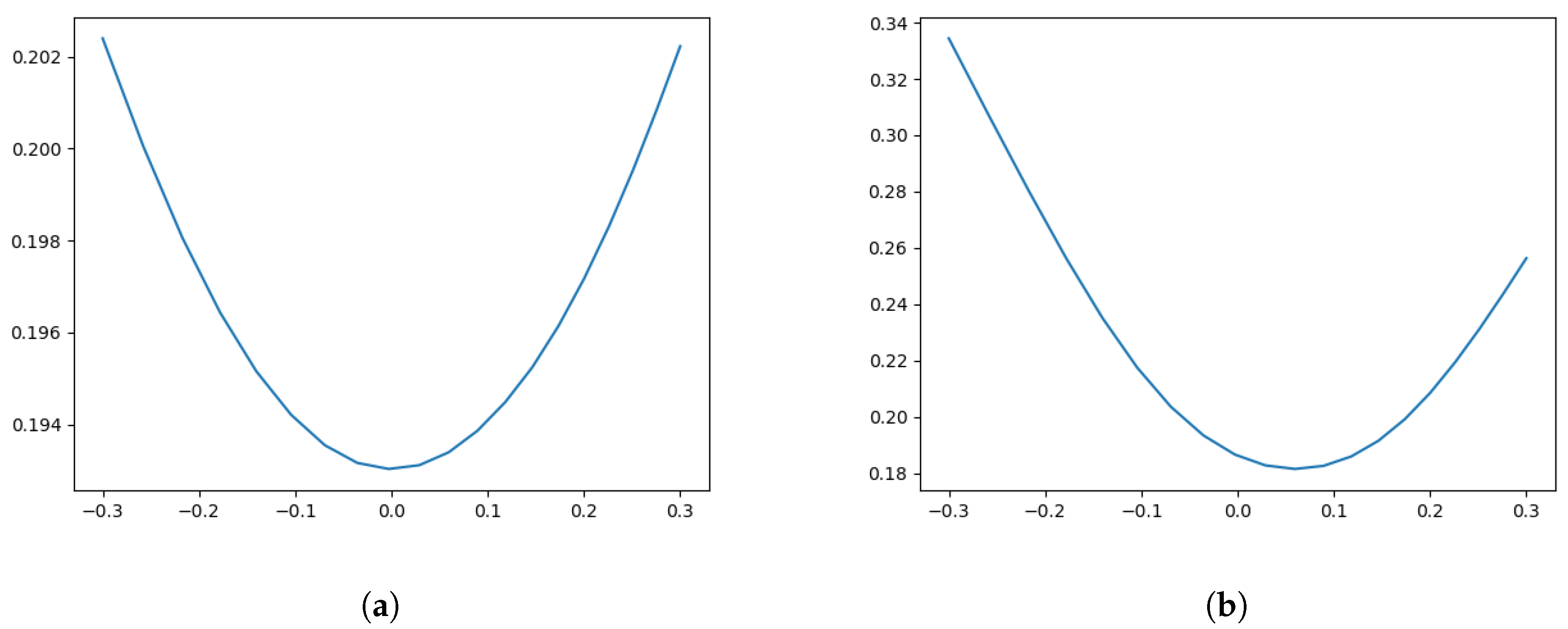
In Figure 1a we show plots of implied volatilities for different slices (maturities) for a realistic choice of parameters. As one can see, the produced smiles seem to be unrealistically flat. Hence we modify the local volatility function a ˜ ξ to produce more pronounced and more realistic smiles. To be precise, we define a new family of local volatility functions a ξ indexed by the set of parameters ξ as
a ξ 2 ( t , x ) = 1 4 × min ( 2 , i = 0 2 p i σ i k ( t , x , σ i ) + Λ ( t , x ) 1 0.6 × 1 t > 0.1 i = 0 2 ( p i / σ i ) k ( t , x , σ i ) + 0.01 ) ,
with
Λ ( t , x ) : = 1 t 0.1 1 + 0.1 t λ 2 min γ 1 x β 1 + + γ 2 x β 2 + κ , λ 1 .
We fix the choice of the parameters γ i , β i , λ i , κ as given in Table 1. By taking absolute values above, we can drop the requirement p 0 > 0 which is what we do in the sequel. Please note that a ξ 2 is not defined at t = 0 . When doing a Monte Carlo simulation, we simply replace a ξ 2 ( 0 , x ) with a ξ 2 ( Δ t , x ) , where Δ t is the time increment of the Monte Carlo simulation.
What is left to be specified are the parameters
ξ = ( p 1 , p 2 , σ 0 , σ 1 , σ 2 )
with p 0 = 1 p 1 p 2 . This motivates our statistical test for the performance evaluation of our method. To be precise, our ground truth assumption is that all observable market prices are explained by a variation of the parameters ξ . For illustration, we plot implied volatilities for this modified local volatility function in Figure 1b for a specific parameter set ξ .
Our ground truth model is now specified as in (25) with σ Dup replaced by a ξ , i.e.,
d X t = 1 2 a ξ 2 ( t , X t ) d t + a ξ ( t , X t ) d W t .

4.1.2. Performance Test

We now come to the evaluation of our proposed method. We want to calibrate the SABR-LSV model to synthetic market prices generated by the previously formulated ground truth assumption. This corresponds to randomly sampling the parameter ξ of the local volatility function a ξ and to compute prices according to (27). Calibrating the SABR-LSV model, i.e., finding the parameters ν , ρ , the initial volatility α 0 and the unknown leverage function L, to these prices and repeating this multiple times then allows for a statistical analysis of the errors.
As explained in Section 3, we consider European call options with maturities T 1 < < T n and denote the strikes for a given maturity T i by K i j , j { 1 , , J i } . To compute the ground truth prices for these European calls we use a Euler-discretization of (27) with time step Δ t = 1 / 100 . Prices are then obtained by a variance reduced Monte Carlo estimator using 10 7 Brownian paths and a Black–Scholes delta hedge variance reduction as described previously. For a given parameter set ξ , we use the same Brownian paths for all strikes and maturities.
Overall, in this test, we consider n = 4 maturities with J i = 20 strike prices for all i = 1 , , 4 . The values for T i are given in Figure 2a. For the choice of the strikes K i , we choose evenly spaced points, i.e.,
K i , j + 1 K i , j = K i , 20 K i , 1 19 .
For the smallest and largest strikes per maturity we choose
K i , 1 = exp k i , K i , 20 = exp k i ,
with the values of k i given in Figure 2b.
We now specify a distribution under which we draw the parameters
ξ = ( p 1 , p 2 , σ 0 , σ 1 , σ 2 , )
for our test. The components are all drawn independently from each other under the uniform distribution on the respective intervals given below.
-
I p 1 = [ 0.4 , 0.5 ]
-
I p 2 = [ 0.4 , 0.7 ]
-
I σ 0 = [ 0.5 , 1.7 ]
-
I σ 1 = [ 0.2 , 0.4 ]
-
I σ 2 = [ 0.5 , 1.7 ]
We can now generate data by the following scheme.
  • For m = 1 , , 200 simulate parameters ξ m under the law described above.
  • For each m, compute prices of European calls for maturities T i and strikes K i j for i = 1 , , n = 4 and j = 1 , , 20 according to (27) using 10 7 Brownian trajectories (for each m we use new trajectories).
  • Store these prices.
Remark 3.
In very few cases, the simulated parameters were such that the implied volatility computation for model prices failed at least for one maturity due to the remaining Monte Carlo error. In those cases, we simply skip that sample and continue with the next, meaning that we will perform the statistical test only on the samples for which these implied volatility computations were successful.
The second part consists of calibrating each of these surfaces and storing pertinent values for which we conduct a statistical analysis. In the following we describe the procedure in detail:
Recall that we specify the leverage function L ( t , x ) via a family of neural networks, i.e.,
L ( t , x ) = 1 + F i ( x ) t [ T i 1 , T i ) , i { 1 , , n = 4 } ,
where F i NN 1 , 1 (see Notation A1). Each F i is specified as a 4-hidden layer feed-forward network where the dimension of each of the hidden layers is 64. As activation function we choose leaky-ReLU4 with parameter 0.2 for the first three hidden layers and ϕ = tanh for the last hidden layer. This choice means of course a considerable overparameterization, where we deal with much more parameters than data points. As is well known from the theory of machine learning, this however allows a profit to be made from implicit regularizations for the leverage function, meaning that the variations of higher derivatives are small.
Remark 4.
In our experiments, we tested different network architectures. Initially, we used networks with three to five hidden layers with layer dimensions between 50 and 100 and activation function tanh in all layers. Although the training was successful, we observed that training was significantly slower with significant lower calibration accuracy compared to the final architecture. We also tried classical ReLU, but observed that the training sometimes got stuck due to flat gradients. In case of pure leaky-ReLU activation functions, we observed numerical instabilities. By adding a final tanh activation, this computation was regularized leading to the results we present here.
Since closed form pricing formulas are not available for such an LSV model, let us briefly specify our pricing method. For the variance reduced Monte Carlo estimator as of (21) we always use a standard Euler-SDE discretization with step size Δ t = 1 / 100 . As variance reduction method, we implement the running Black–Scholes Delta hedge with instantaneous running volatility of the price process, i.e., L ( t , X t ) α t is plugged in the formula for the Black–Scholes Delta as in (9). The only parameter that remains to be specified, is the number of trajectories used for the Monte Carlo estimator which is done in Algorithms A1 and A2 below.
As a first calibration step, we calibrate the SABR model (i.e., (1) with L 1 ) to the synthetic market prices of the first maturity and fix the calibrated SABR parameters ν , ρ and α 0 . This calibration is not done by the SABR formula, but rather in the same way the LSV model calibration is implemented: we use a Monte Carlo simulation based engine where gradients are computed via backpropagation. The calibration objective function is analog to (21) and we compute the full gradient as specified in (23). We only use a maximum of 2000 trajectories and the running Black–Scholes hedge for variance reduction per gradient computation, as we are only interested in an approximate fit. In fact, when compared to a better initial SABR fit achieved by the SABR formula, we observed that the calibration fails more often due to local minima becoming an issue.
For training the parameters θ i , i = 1 , , 4 , of the neural networks we apply Algorithm A1 in the Appendix D.

4.2. Numerical Results for the Calibration Test

We now discuss the results of our test. We start by pointing out that from the 200 synthetic market smiles generated, four smiles caused difficulties, in the sense that our implied volatility computation failed due to the remaining Monte Carlo error in the model price computation, compare Remark 3. By increasing the training parameters slightly (in particular the number of trajectories used in the training), this issue can be mitigated but the resulting calibrated implied volatility errors stay large out of the money where the smiles are extreme, and the training will take more time. Hence, we opt to remove those four samples from the following statistical analysis as they represented unrealistic market smiles.
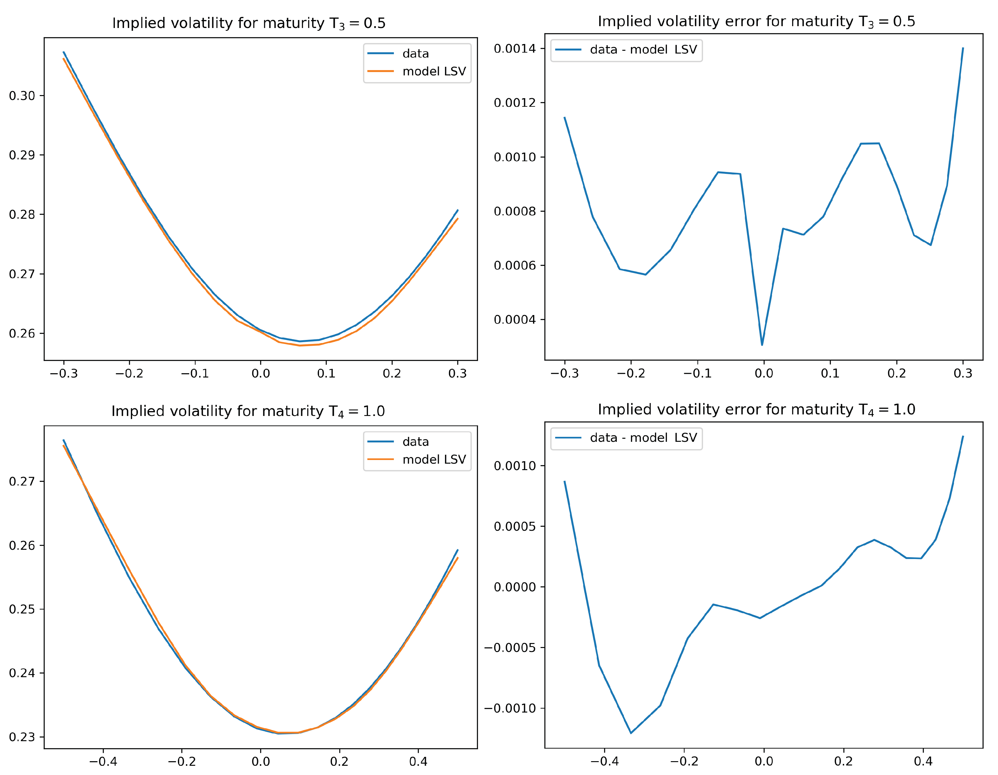
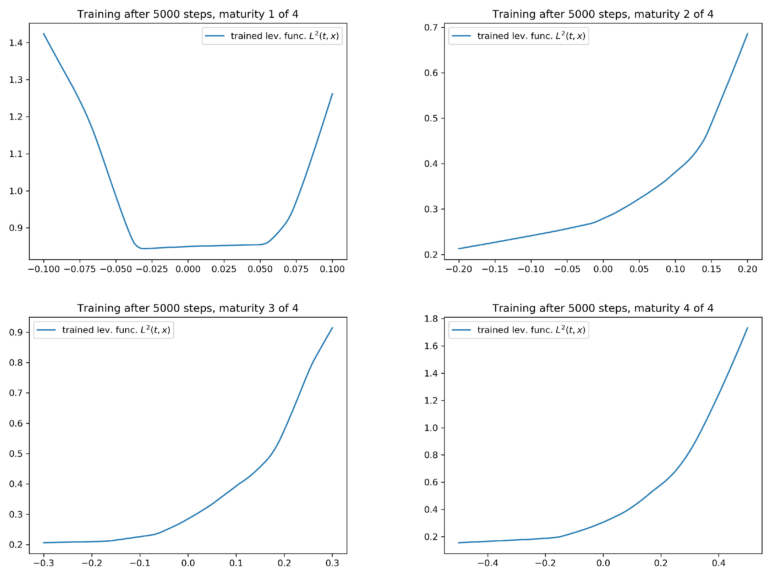
In Figure 3 we show calibration results for a typical example of randomly generated synthetic market data. From this it is already visible that the worst-case calibration error (which occurs out of the money) ranges typically between 5 and 15 basis points. The corresponding calibration result for the square of the leverage function L 2 is given in Figure 4.
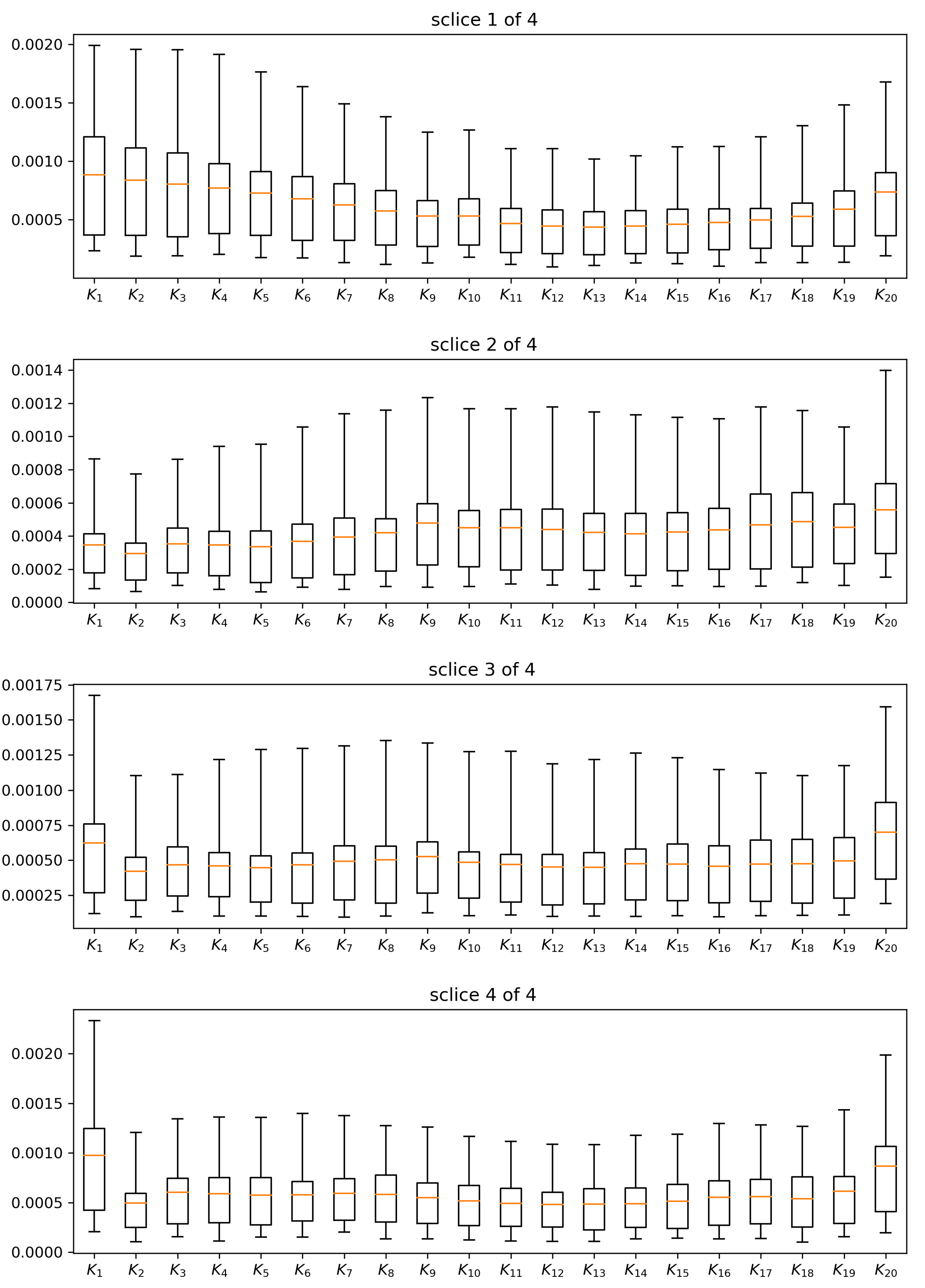
Let us note that our method achieves a very high calibration accuracy for the considered range of strikes across all considered maturities. This can be seen in the results of a worst-case analysis of calibration errors in Figure 5. There we show the mean as well as different quantiles of the data. Please note that the mean always lies below 10 basis point across all strikes and maturities.
Regarding calibration times, we can report that from the 196 samples, 191 finished within 26 to 27 min. In all these cases, the abort criterion was active on the first time it was checked, i.e., after 5000 iterations. The other five samples are examples of smiles comparable to the four where implied volatility computation itself failed. In those cases, more iteration steps where needed resulting in times between 46 and 72 min. These samples also correspond to the less successful calibration results.
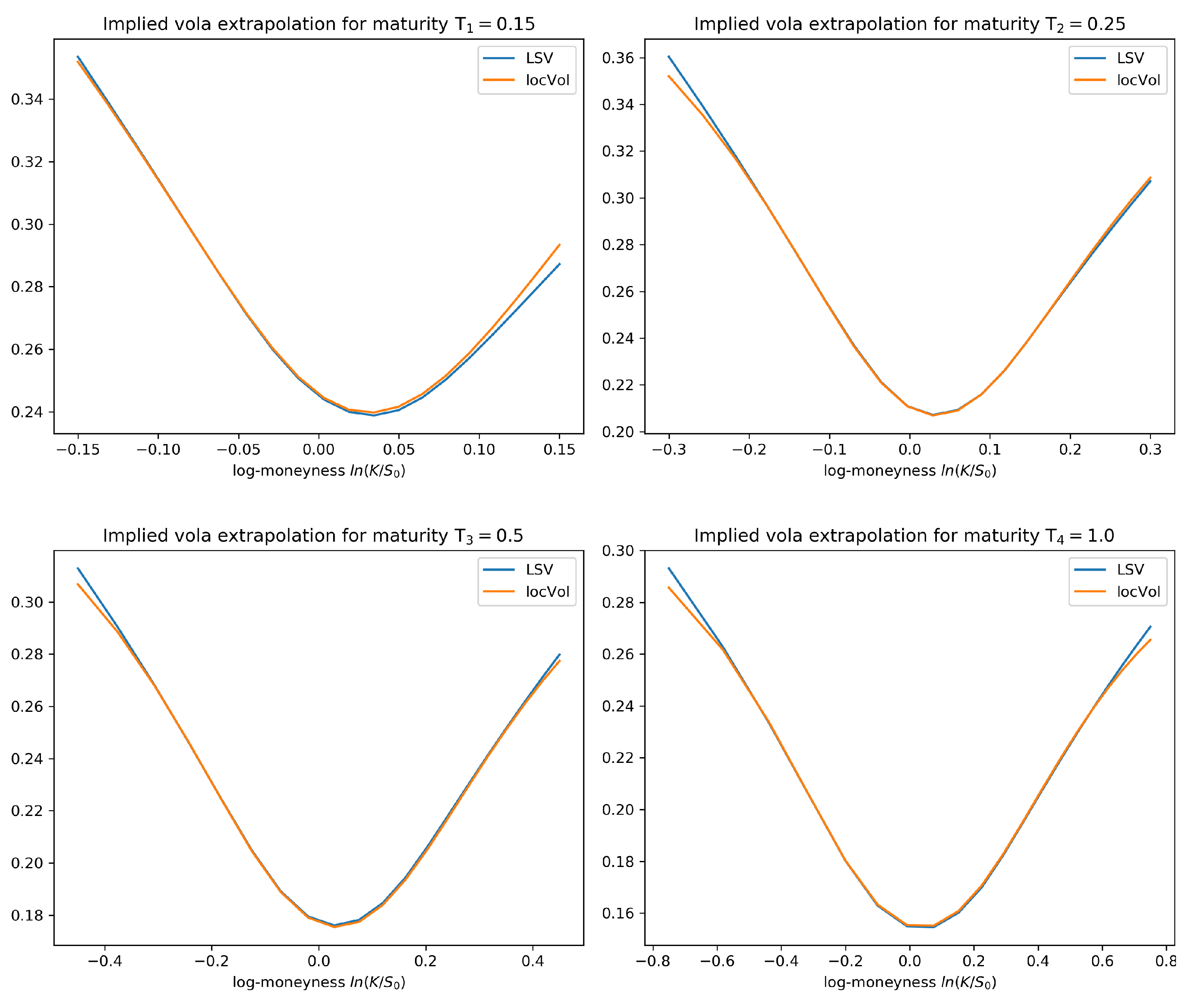
To perform an out of sample analysis, we check for extra- and interpolation properties of the learned leverage function. This means that we compute implied volatilities on an extended range and compare to the implied volatility of the ground truth assumption. The strikes of these ranges are again computed by taking 20 equally spaced points as before, but with parameters k i as of table Figure 2b multiplied with 1.5. This has also the effect that the strikes inside the original range do not correspond to the strikes considered during training, which allows for an additional analysis of the interpolation properties. These results are illustrated in Figure 6, from which we see that extrapolation is very close to the local volatility model.

4.3. Robust Calibration—An Instance of the Adversarial Approach

Let us now describe a robust version of our calibration methodology realized in an adversarial manner. We start by assuming that there are multiple “true” option prices which correspond to the bid-ask spreads observed on the market. The way we realize this in our experiment is to use several local volatility functions that generate equally plausible market implied volatilities. Recall that the local volatility functions in our statistical test above are functions of the parameters ( p 0 , p 1 , σ 0 , σ 1 , σ 2 ) . We fix these parameters and generate 4 smiles from local volatility functions with slightly perturbed parameters
( p 0 + u i 1 , p 1 + u i 2 , σ 0 + u i 3 , σ 1 + u i 4 , σ 2 + u i 5 ) for i = 1 , , 4 ,
where u i j are i.i.d. uniformly distributed random variables, i.e., u i j U [ u , u ] with u = 0.01 . The loss function for maturity T i in the training part now changes to
inf θ j = 1 J i w j sup m = 1 , , 4 1 N n = 1 N X j , m ( θ ) ( ω n ) ,
with X j , m defined as X j in (20) (see also (17)) but with synthetic market prices m = 1 , , 4 generated by the m-th local volatility function. We are thus in an adversarial situation as described in the introduction: we have several possibilities for the loss function corresponding to the different market prices and we take the supremum over these (individually for each strike). In our toy example we can simply compute the gradient of this supremum function with respect to θ . In a more realistic situation, where we do not only have 4 smiles but a continuum we would iterate the inf and sup computation, meaning that we would also perform a gradient step with respect to m. This corresponds exactly to the adversary part. For a given parameter set θ , the adversary tries to find the worst loss function.
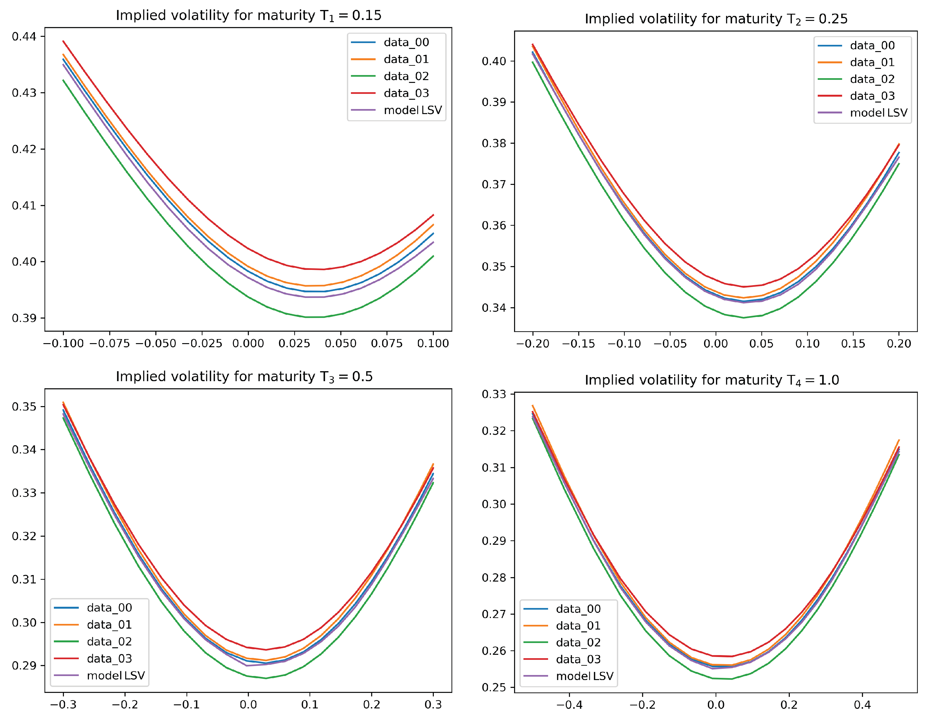
In Figure 7, we illustrate the result of this robust calibration, where find that the calibrated model lies between the four different smiles over which we take the supremum.

5. Conclusions

We have demonstrated how the parametrization by means of neural networks can be used to calibrate local stochastic volatility models to implied volatility data. We make the following remarks:
  • The method we presented does not require any form of interpolation for the implied volatility surface since we do not calibrate via Dupire’s formula. As the interpolation is usually done ad hoc, this might be a desirable feature of our method.
  • Similar to Guyon and Henry-Labordѐre (2012); Guyon and Henry-Labordѐre (2013), it is possible to “plug in” any stochastic variance process such as rough volatility processes as long as an efficient simulation of trajectories is possible.
  • The multivariate extension is straight forward.
  • The level of accuracy of the calibration result is of a very high degree. The average error in our statistical test is of around 5 to 10 basis points, which is an interesting feature in its own right. We also observe good extrapolation and generalization properties of the calibrated leverage function.
  • The method can be significantly accelerated by applying distributed computation methods in the context of multi-GPU computational concepts.
  • The presented algorithm is further able to deal with path-dependent options since all computations are done by means of Monte Carlo simulations.
  • We can also consider the instantaneous variance process of the price process as short end of a forward variance process, which is assumed to follow (under appropriate assumptions) a neural SDE. This setting, as an infinite-dimensional version of the aforementioned “multivariate” setting, then qualifies for joint calibration to S&P and VIX options. This is investigated in a companion paper.
  • We stress again the advantages of the generative adversarial network point of view. We believe that this is a crucial feature in the joint calibration of S&P and VIX options.

6. Plots

This section contains the relevant plots for the numerical test outlined in Section 4.

Author Contributions

All authors have contributed in equal parts. All authors have read and agreed to the published version of the manuscript.

Funding

Christa Cuchiero gratefully acknowledges financial support by the Vienna Science and Technology Fund (WWTF) under grant MA16-021 and by the FWF under grant I 3852-N32.

Conflicts of Interest

The authors declare no conflict of interest.

Appendix A. Variations of Stochastic Differential Equations

We follow here the excellent exposition of Protter (1990) to understand the dependence of solutions of stochastic differential equations on parameters, in particular when we aim to calculate derivatives with respect to parameters of neural networks.
Let us denote by D the set of real-valued, càdlàg, adapted processes on a given stochastic basis ( Ω , F , Q ) with a filtration (satisfying usual conditions). By D n we denote the set of R n -valued, càdlàg, adapted processes on the same basis.
Definition A1.
An operator F from D n to D is called functional Lipschitz if for any X , Y D n
1. 
the property X τ = Y τ implies F ( X ) τ = F ( Y ) τ for any stopping time τ,
2. 
there exists an increasing process ( K t ) t 0 such that for t 0
F ( X ) t F ( Y ) t K t sup r t X r Y r .
Functional Lipschitz assumptions are sufficient to obtain existence and uniqueness for general stochastic differential equations, see (Protter 1990, Theorem V 7).
Theorem A1.
Let Y = ( Y 1 , , Y d ) be a vector of semimartingales starting at Y 0 = 0 , ( J 1 , , J n ) D n a vector of processes and let F j i , i = 1 , , n , j = 1 , , d be functionally Lipschitz operators. Then there is a unique process Z D n satisfying
Z t i = J t i + j = 1 d 0 t F j i ( Z ) s d Y s j
for t 0 and i = 1 , , n . If J is a semimartingale, then Z is a semimartingale as well.
With an additional uniformity assumption on a sequence of stochastic differential equations with converging coefficients and initial data we obtain stability, see (Protter 1990, Theorem V 15).
Theorem A2.
Let Y = ( Y 1 , , Y d ) be vector of semimartingales starting at Y 0 = 0 . Consider for ε 0 , a vector of processes ( J ε , 1 , , J ε , n ) D n and functionally Lipschitz operators F j ε , i for i = 1 , , n , j = 1 , , d . Then, for ε 0 , there is a unique process Z ε D n satisfying
Z t ε , i = J t ε , i + j = 1 d 0 t F j ε , i ( Z ε ) s d Y s j
for t 0 and i = 1 , , n . If J ε J 0 in ucp, F ε ( Z 0 ) F 0 ( Z 0 ) in ucp, then Z ε Z 0 in ucp.
Remark A1.
We shall apply these theorems to a local stochastic volatility model of the form
d S t ( θ ) = S t ( θ ) L ( t , S t ( θ ) , θ ) α t d W t ,
where θ Θ , ( W , α ) denotes some Brownian motion together with an adapted, càdlàg stochastic process α (all on a given stochastic basis) and S 0 > 0 is some real number.
We assume that for each θ Θ
( t , s ) L ( t , s , θ )
is bounded, càdlàg in t (for fixed s > 0 ), and globally Lipschitz in s with a Lipschitz constant independent of t on compact intervals. In this case, the map
S S · L ( · , S · , θ )
is functionally Lipschitz and therefore the above equation has a unique solution for all times t and any θ by Theorem A1. If, additionally,
lim θ θ ^ sup ( t , s ) | L ( t , s , θ ) L ( t , s , θ ^ ) | = 0 ,
where the sup is taken over some compact set, then we also have that the solutions S ( θ ) converge ucp to S ( θ ^ ) , as θ θ ^ by Theorem A2.

Appendix B. Preliminaries on Deep Learning

We shall here briefly introduce two core concepts in deep learning, namely artificial neural networks and stochastic gradient descent. The latter is a widely used optimization method for solving maximization or minimization problems involving the first. In standard machine-learning terminology, the optimization procedure is usually referred to as “training”. We shall use both terminologies interchangeably.

Appendix B.1. Artificial Neural Networks

We start with the definition of feed-forward neural networks. These are functions obtained by composing layers consisting of an affine map and a componentwise nonlinearity. They serve as universal approximation class which is stated in Theorem A3. Moreover, derivatives of these functions can be efficiently expressed iteratively (see e.g., Hecht-Nielsen (1992)), which is a desirable feature from an optimization point of view.
Definition A2.
Let M , N 0 , N 1 , , N M N , ϕ : R R and for any m { 1 , , M } , let w m : R N m 1 R N m , x A m x + b m be an affine function with A m R N m × N m 1 and b m R N m . A function R N 0 R N M defined as
F ( x ) = w M F M 1 F 1 , with F m = ϕ w m for m { 1 , , M 1 }
is called a feed-forward neural network. Here the activation function ϕ is applied componentwise. M 1 denotes the number of hidden layers and N 1 , , N M 1 denote the dimensions of the hidden layers and N 0 and N M the dimension of the input and output layers.
Remark A2.
Unless otherwise stated, the activation functions ϕ used in this article are always assumed to be smooth, globally bounded with bounded first derivative.
The following version of the so-called universal approximation theorem is due to K. Hornik (Hornik 1991). An earlier version was proved by G. Cybenko (Cybenko 1989). To formulate the result, we denote the set of all feed-forward neural networks with activation function ϕ , input dimension N 0 and output dimension N M by NN , N 0 , N M ϕ .
Theorem A3
(Hornik (1991)). Suppose ϕ is bounded and nonconstant. Then the following statements hold:
1. 
For any finite measure μ on ( R N 0 , B ( R N 0 ) ) and 1 p < , the set NN , N 0 , 1 ϕ is dense in L p ( R N 0 , B ( R N 0 ) , μ ) .
2. 
If in addition ϕ C ( R , R ) , then NN , N 0 , 1 ϕ is dense in C ( R N 0 , R ) for the topology of uniform convergence on compact sets.
Since each component of an R N M -valued neural network is an R -valued neural network, this result easily generalizes to NN , N 0 , N M ϕ with N M > 1 .
Notation A1.
We denote by NN N 0 , N M the set of all neural networks in NN , N 0 , N M ϕ with a fixed architecture, i.e., a fixed number of hidden layers M 1 , fixed input and output dimensions N m for each hidden layer m { 1 , , M 1 } and a fixed activation function ϕ. This set can be described by
NN N 0 , N M = { F ( · , θ ) | F feed forward neural network and θ Θ } ,
with parameter space Θ R q for some q N and θ Θ corresponding to the entries of the matrices A m and the vectors b m for m { 1 , , M } .

Appendix B.2. Stochastic Gradient Descent

In light of Theorem A3, it is clear that neural networks can serve as function approximators. To implement this, the entries of the matrices A m and the vectors b m for m { 1 , , M } are subject to optimization. If the unknown function can be expressed as the expected value of a stochastic objective function, one widely applied optimization method is stochastic gradient descent, which we shall review below.
Indeed, consider the following minimization problem
min θ Θ f ( θ ) with f ( θ ) = E [ Q ( θ ) ]
where Q denotes some stochastic objective function5 Q : Ω × Θ R , ( ω , θ ) Q ( θ ) ( ω ) that depends on parameters θ taking values in some space Θ .
The classical method how to solve generic optimization problems for some differentiable objective function f (not necessarily of the expected value form as in (A3)) is to apply a gradient descent algorithm: starting with an initial guess θ ( 0 ) , one iteratively defines
θ ( k + 1 ) = θ ( k ) η k f ( θ ( k ) )
for some learning rate η k . Under suitable assumptions, θ ( k ) converges for k to a local minimum of the function f.
In the deep learning context, stochastic gradientdescent methods, going back to stochastic approximation algorithms proposed by Robbins and Monro (1951), are much more efficient. To apply this, it is crucial that the objective function f is linear in the sampling probabilities. In other words, f needs to be of the expected value form as in (A3). In the simplest form of stochastic gradient descent, under the assumption that
f ( θ ) = E [ Q ( θ ) ] ,
the true gradient of f is approximated by a gradient at a single sample Q ( θ ) ( ω ) which reduces the computational cost considerably. In the updating step for the parameters θ as in (A4), f is then replaced by Q ( θ ) ( ω k ) , hence
θ ( k + 1 ) = θ ( k ) η k Q ( θ ( k ) ) ( ω k ) .
The algorithm passes through all samples ω k of the so-called training data set, possibly several times (specified by the number of epochs), and performs the update until an approximate minimum is reached.
A compromise between computing the true gradient of f and the gradient at a single sample Q ( θ ) ( ω ) is to compute the gradient of a subsample of size N batch , called (mini)-batch, so that Q ( θ ( k ) ) ( ω k ) used in the update (A5) is replaced by
Q ( k ) ( θ ) = 1 N batch n = 1 N batch Q ( θ ) ( ω n + k N batch ) , k { 0 , 1 , . . . , N / N batch 1 } ,
where N is the size of the whole training data set. Any other unbiased estimators of f ( θ ) can of course also be applied in (A5).

Appendix C. Alternative Approaches for Minimizing the Calibration Functional

We consider here alternative algorithms for minimizing (18).

Appendix C.1. Stochastic Compositional Gradient Descent

One alternative is stochastic compositional gradient descent as developed e.g., in Wang et al. (2017). Applied to our problem this algorithm (in its simplest form) works as follows: starting with an initial guess θ ( 0 ) , and y j ( 0 ) , j = 1 , , J one iteratively defines
y j ( k + 1 ) = ( 1 β k ) y j ( k ) + β k Q j ( θ ( k ) ) ( ω k ) j = 1 , , J , θ ( k + 1 ) = θ ( k ) η k j = 1 J w j ( y j ( k + 1 ) ) Q j ( θ ( k ) ) ( ω k )
for some learning rates β k , η k ( 0 , 1 ] . Please note that y ( k ) is an auxiliary variable to track the quantity E [ Q ( θ ( k ) ) ] which has to be plugged in (other faster converging estimates have also been developed). Of course Q j ( θ ( k ) ) ( ω k ) can also be replaced by other unbiased estimates of the gradient, e.g., the gradient of the (mini)-batches as in (A6). For convergence results in the case when θ ( E [ Q j ( θ ) ] ) is convex we refer to (Wang et al. 2017, Theorem 5). Of course, the same algorithm can be applied when we replace Q j ( θ ) in (18) with X j ( θ ) as defined in (20) for the variance reduced case.

Appendix C.2. Estimators Compatible with Stochastic Gradient Descent

Our goal here is to apply at least in special cases of the nonlinear function (variant (A6) of) stochastic gradient descent to the calibration functional (18). This means that we must cast (18) into expected value form. We focus on the case when ( x ) is given by ( x ) = x 2 and write f ( θ ) as
f ( θ ) = j = 1 J w j E Q j ( θ ) Q ˜ j ( θ )
for some independent copy Q ˜ j ( θ ) of Q j ( θ ) , which is clearly of the expected value form required in (A3). A Monte Carlo estimator of f ( θ ) is then constructed by
f ^ ( θ ) = 1 N n = 1 N j = 1 J w j Q j ( θ ) ( ω n ) Q ˜ j ( θ ) ( ω n ) .
for independent draws ω 1 , , ω N (the same N samples can be used for each strike K j ). Equivalently we have
f ^ ( θ ) = 1 N n = 1 N j = 1 J w j Q j ( θ ) ( ω n ) Q j ( θ ) ( ω n + m ) .
for independent draws ω 1 , , ω 2 N . The analog of (A6) is then given by
Q ( k ) ( θ ) = 1 N batch l = 1 N batch j = 1 J w j Q j ( θ ) ( ω l + 2 k N batch ) Q j ( θ ) ( ω l + ( 2 k + 1 ) N batch )
for k { 0 , 1 , . . . , N / N batch 1 } .
Clearly we can now modify and improve the estimator by using again hedge control variates and replace Q j ( θ ) by X j ( θ ) as defined in (20).

Appendix D. Algorithms

In this section, we present the calibration algorithm discussed above in form of pseudo code given in Algorithm A1. Update rules for parameters in Algorithm A1 are provided in Algorithm A2. We further provide an implementation in form of a github repository, see https://github.com/wahido/neural_locVol.
Algorithm A1: In the subsequent pseudo code, the index i stands for the maturities, N for the number of samples used in the variance reduced Monte Carlo estimator as of (21) and k for the updating step in the gradient descent:
1 # Initialize the network parameters
2 initialize  θ1,…θ4
3 # Define initial number of trajectories and initial step
4 N, k = 400, 1
5 # The time discretization for the MC simulations and the
6 # abort criterion
7 Δt, tol = 0.01, 0.0045
8  
9 for i = 1,...,4:
10   nextslice = False
11   # Compute the initial normalized vega weights for this slice:
12  wj = j/ l = 1 20 l with j = 1/vij,  where vij is the Black-Scholes
13   vega for strike Kij, the corresponding synthetic market implied
14   volatility and the maturity Ti.
15  
16 while nextslice == False:
17   do:
18     Simulate N trajectories of the SABR-LSV process up
19     to time Ti, compute the payoffs.
20   do:
21     Compute the stochastic integral of the Black-Scholes
22     Delta hedge against these trajectories as of (9)
23     for maturity Ti
24   do:
25     Compute the calibration functional as of (21)
26     with ℓ(x) = x2 and  weights wj  with the modification that we use put
27     options instead of call options for strikes larger than the spot.
28   do:
29     Make an optimization step from  θ i ( k 1 )  to  θ i ( k ) , similarly
30     as in (22) but with the more sophisticated ADAM-
31     optimizer with learning rate 10−3.
32   do:
33     Update the parameter N, the condition nextslice and
34     compute model prices according to Algorithm A2.
35   do:
36     k = k + 1
Algorithm A2: We update the parameters in Algorithm A1 according to the following rules:
1       if k == 500:
2         N = 2000
3       else if k == 1500:
4         N = 10000
5       else if k == 4000:
6         N = 50000
7  
8       if k >= 5000 and k mod 1000 == 0:
9         do:
10           Compute model prices πmodel for slice i via MC simulation
11           using 107 trajectories. Apply the Black-Scholes Delta
12           hedge for variance reduction.
13         do:
14           Compute implied volatilities ivmodel from the model prices πmodel.
15         do:
16           Compute the maximum error of model implied volatilities
17           against synthetic market implied volatilities:
18           err_cali = ‖iv_model - iv_market‖max
19           if err_cali ≤ tol or k == 12000:
20             nextslice = True
21           else:
22             Apply the adversarial part: Adjust the weights wj
23             according to:
24  
25             for j = 1,…,20:
26               wj = wj + ∣iv_modelj - iv_marketj
27             This puts higher weights on the options where the fit
28             can still be improved
29             Normalize the weights:
30             for j = 1,…,20:
31               wj = wj /  Σ 𝓁 = 1 20  w

References

  1. Abergel, Frédéric, and Rémi Tachet. 2010. A nonlinear partial integro-differential equation from mathematical finance. Discrete and Continuous Dynamical Systems-Series A 27: 907–17. [Google Scholar] [CrossRef]
  2. Acciaio, Beatrice, and Tianlin Xu. 2020. Learning Dynamic GANs via Causal Optimal Transport. Working paper. [Google Scholar]
  3. Bayer, Christian, Blanka Horvath, Aitor Muguruza, Benjamin Stemper, and Mehdi Tomas. 2019. On deep calibration of (rough) stochastic volatility models. arXiv arXiv:1908.08806. [Google Scholar]
  4. Becker, Sebastian, Patrick Cheridito, and Arnulf Jentzen. 2019. Deep optimal stopping. Journal of Machine Learning Research 20: 1–25. [Google Scholar]
  5. Bühler, Hans, Lukas Gonon, Josef Teichmann, and Ben Wood. 2019. Deep hedging. Quantitative Finance 19: 1271–91. [Google Scholar] [CrossRef]
  6. Bühler, Hans, Blanka Horvath, Immanol Perez Arribaz, Terry Lyons, and Ben Wood. 2020. A Data-Driven Market Simulator for Small Data Environments. Available online: https://ssrn.com/abstract=3632431 (accessed on 22 September 2020).
  7. Carmona, René, and Sergey Nadtochiy. 2009. Local volatility dynamic models. Finance and Stochastics 13: 1–48. [Google Scholar] [CrossRef] [Green Version]
  8. Carmona, Rene, Ivar Ekeland, Arturo Kohatsu-Higa, Jean-Michel Lasry, Pierre-Louis Lions, Huyen Pham, and Erik Taflin. 2007. HJM: A Unified Approach to Dynamic Models for Fixed Income, Credit and Equity Markets. Berlin/Heidelberg: Springer, vol. 1919, pp. 1–50. [Google Scholar] [CrossRef]
  9. Cont, Rama, and Sana Ben Hamida. 2004. Recovering volatility from option prices by evolutionary optimization. Journal of Computational Finance 8: 43–76. [Google Scholar] [CrossRef] [Green Version]
  10. Cozma, Andrei, Matthieu Mariapragassam, and Christoph Reisinger. 2019. Calibration of a hybrid local-stochastic volatility stochastic rates model with a control variate particle method. SIAM Journal on Financial Mathematics 10: 181–213. [Google Scholar] [CrossRef]
  11. Cuchiero, Christa, Alexia Marr, Milusi Mavuso, Nicolas Mitoulis, Aditya Singh, and Josef Teichmann. 2018. Calibration of Mixture Interest Rate Models with Neural Networks. Technical report. [Google Scholar]
  12. Cuchiero, Christa, Philipp Schmocker, and Teichmann Josef. 2020. Deep Stochastic Portfolio Theory. Working paper. [Google Scholar]
  13. Cybenko, George. 1992. Approximation by superpositions of a sigmoidal function. Mathematics Control, Signal and Systems 2: 303–14. [Google Scholar] [CrossRef]
  14. Dupire, Bruno. 1994. Pricing with a smile. Risk 7: 18–20. [Google Scholar]
  15. Dupire, Bruno. 1996. A unified theory of volatility. In Derivatives Pricing: The Classic Collection. London: Risk Books, pp. 185–96. [Google Scholar]
  16. Eckstein, Stephan, and Michael Kupper. 2019. Computation of optimal transport and related hedging problems via penalization and neural networks. Applied Mathematics & Optimization, 1–29. [Google Scholar] [CrossRef] [Green Version]
  17. Gao, Xiaojie, Shikui Tu, and Lei Xu. 2019. A tree search for portfolio management. arXiv arXiv:1901.01855. [Google Scholar]
  18. Gatheral, Jim, Thibault Jaisson, and Mathieu Rosenbaum. 2018. Volatility is rough. Quantitative Finance 18: 933–49. [Google Scholar] [CrossRef]
  19. Gierjatowicz, Patryk, Mark Sabate, David Siska, and Lukasz Szpruch. 2020. Robust Pricing and Hedging via Neural SDEs. Available online: https://papers.ssrn.com/sol3/papers.cfm?abstract_id=3646241 (accessed on 22 September 2020).
  20. Goodfellow, Ian, Jean Pouget-Abadie, Mehdi Mirza, Bing Xu, David Warde-Farley, Sherjil Ozair, Aaron Courville, and Yoshua Bengio. 2014. Generative adversarial nets. In Advances in Neural Information Processing Systems. Cambridge: The MIT Press, pp. 2672–80. [Google Scholar]
  21. Guyon, Julien, and Pierre Henry-Labordère. 2012. Being particular about calibration. Risk 25: 92–97. [Google Scholar]
  22. Guyon, Julien, and Pierre Henry-Labordère. 2013. Nonlinear Option Pricing. Chapman & Hall/CRC Financial Mathematics Series. [Google Scholar]
  23. Guyon, Julien. 2014. Local correlation families. Risk. February, pp. 52–58. Available online: https://search.proquest.com/openview/c1bb3fbf83b00ad34eaeeee071f0be52/1?pq-origsite=gscholar&cbl=32048 (accessed on 20 September 2020).
  24. Guyon, Julien. 2016. Cross-dependent volatility. Risk 29: 61–65. [Google Scholar] [CrossRef] [Green Version]
  25. Han, Jiequn, Arnulf Jentzen, and Weinan E. 2017. Overcoming the curse of dimensionality: Solving high-dimensional partial differential equations using deep learning. arXiv arXiv:1707.02568. [Google Scholar]
  26. Hecht-Nielsen, Robert. 1989. Theory of the backpropagation neural network. Paper presented at International 1989 Joint Conference on Neural Networks, Washington, DC, USA; vol. 1, pp. 593–605. [Google Scholar] [CrossRef]
  27. Heiss, Jakob, Josef Teichmann, and Hanna Wutte. 2019. How implicit regularization of neural networks affects the learned function–part i. arXiv arXiv:1911.02903. [Google Scholar]
  28. Henry-Labordère, Pierre. 2019. Generative Models for Financial Data. Preprint. Available online: https://ssrn.com/abstract=3408007 (accessed on 22 September 2020).
  29. Hernandez, Andres. 2017. Model calibration with neural networks. Risk. [Google Scholar] [CrossRef] [Green Version]
  30. Hornik, Kurt. 1991. Approximation capabilities of multilayer feedforward networks. Neural Networks 4: 251–57. [Google Scholar] [CrossRef]
  31. Huré, Côme, Huyên Pham, Achref Bachouch, and Nicolas Langrené. 2018. Deep neural networks algorithms for stochastic control problems on finite horizon, part i: Convergence analysis. arXiv arXiv:1812.04300. [Google Scholar]
  32. Huré, Côme, Huyên Pham, and Xavier Warin. 2019. Some machine learning schemes for high-dimensional nonlinear PDEs. arXiv arXiv:1902.01599. [Google Scholar]
  33. Jex, Mark, Robert Henderson, and David Wang. 1999. Pricing Exotics under the Smile. Risk Magazine 12: 72–75. [Google Scholar]
  34. Jourdain, Benjamin, and Alexandre Zhou. 2016. Existence of a calibrated regime switching local volatility model and new fake brownian motions. arXiv arXiv:1607.00077. [Google Scholar]
  35. Kondratyev, Alexei, and Christian Schwarz. 2019. The Market Generator. Available online: https://ssrn.com/abstract=3384948 (accessed on 22 September 2020).
  36. Lacker, Dan, Misha Shkolnikov, and Jiacheng Zhang. 2019. Inverting the Markovian projection, with an application to local stochastic volatility models. arXiv arXiv:1905.06213. [Google Scholar]
  37. Lipton, Alexander. 2002. The vol smile problem. Risk Magazine 15: 61–65. [Google Scholar]
  38. Liu, Shuaiqiang, Anastasia Borovykh, Lech Grzelak, and Cornelis Oosterlee. 2019a. A neural network-based framework for financial model calibration. Journal of Mathematics in Industry 9: 9. [Google Scholar] [CrossRef]
  39. Liu, Shuaiqiang, Cornelis Oosterlee, and Sander Bohte. 2019b. Pricing options and computing implied volatilities using neural networks. Risks 7: 16. [Google Scholar] [CrossRef] [Green Version]
  40. Potters, Marc, Jean-Philippe Bouchaud, and Dragan Sestovic. 2001. Hedged Monte-Carlo: Low Variance Derivative Pricing with Objective Probabilities. Physica A: Statistical Mechanics and Its Applications 289: 517–25. [Google Scholar] [CrossRef] [Green Version]
  41. Protter, Philip. 1990. Stochastic Integration and Differential Equations. Volume 21 of Applications of Mathematics (New York). A New Approach. Berlin: Springer. [Google Scholar]
  42. Ren, Yong, Dilip Madan, and Michael Qian Qian. 2007. Calibrating and pricing with embedded local volatility models. London Risk Magazine Limited 20: 138. [Google Scholar]
  43. Robbins, Herbert, and Sutton Monro. 1951. A stochastic approximation method. The Annals of Mathematical Statistics 22: 400–407. [Google Scholar] [CrossRef]
  44. Ruf, Johannes, and Weiguan Wang. Forthcoming. Neural networks for option pricing and hedging: A literature review. Journal of Computational Finance. [CrossRef] [Green Version]
  45. Samo, Yves-Laurent Kom, and Alexander Vervuurt. 2016. Stochastic portfolio theory: A machine learning perspective. arXiv arXiv:1605.02654. [Google Scholar]
  46. Saporito, Yuri F, Xu Yang, and Jorge Zubelli. 2019. The calibration of stochastic-local volatility models-an inverse problem perspective. Computers & Mathematics with Applications 77: 3054–67. [Google Scholar]
  47. Sirignano, Justin, and Rama Cont. 2019. Universal features of price formation in financial markets: Perspectives from deep learning. Quantitative Finance 19: 1449–59. [Google Scholar] [CrossRef]
  48. Tian, Yu, Zili Zhu, Geoffrey Lee, Fima Klebaner, and Kais Hamza. 2015. Calibrating and pricing with a stochastic-local volatility model. Journal of Derivatives 22: 21. [Google Scholar] [CrossRef]
  49. Vidales, Marc-Sabate, David Siska, and Lukasz Szpruch. 2018. Unbiased deep solvers for parametric pdes. arXiv arXiv:1810.05094. [Google Scholar]
  50. Wang, Mengdi, Ethan X Fang, and Han Liu. 2017. Stochastic compositional gradient descent: Algorithms for minimizing compositions of expected-value functions. Mathematical Programming 161: 419–49. [Google Scholar] [CrossRef] [Green Version]
  51. Wiese, Magnus, Lianjun Bai, Ben Wood, and Hans Bühler. 2019. Deep Hedging: Learning to Simulate Equity Option Markets. Available online: https://ssrn.com/abstract=3470756 (accessed on 20 September 2020).
1.
We here use δ to denote the parameters of the hedging neural networks, as θ shall be used for the networks of the leverage function.
2.
This just means that the activation function is bounded and C 1 , with bounded and Lipschitz continuous derivatives.
3.
4.
Recall that ϕ : R R is the leaky-ReLu activation function with parameter α R if ϕ ( x ) = α x 1 ( x < 0 ) + x 1 ( x 0 ) . In particular, classical ReLu is is retrieved by setting α = 0 .
5.
We shall often omit the dependence on ω .
Figure 1. Implied volatility of the original parametric family a ˜ ξ (a) versus our modification a ˜ ξ (b) for maturity T = 0.5, the x-axis is given on log-moneyness ln(K/S0).
Risks 08 00101 g001
Figure 2. Parameters for the synthetic prices to which we calibrate: (a) maturities; (b) parameters that define the strikes for the call options per maturity.
Risks 08 00101 g002
Figure 3. Left column: implied volatilities for the calibrated model together with the data (synthetic market) implied volatilities for a typical example of a synthetic market sample for all available maturities. Right column: calibration errors by subtracting model implied volatilities from the data implied volatilities. The x-axis is given in log-moneyness ln ( K / S 0 ) .
Risks 08 00101 g003aRisks 08 00101 g003b
Figure 4. Plot of the calibrated leverage function x L 2 ( t , x ) at t { 0 , T 1 , T 2 , T 3 } in the example shown in Figure 3. The x-axis is given in log-moneyness ln ( K / S 0 ) .
Risks 08 00101 g004
Figure 5. Boxplots of absolute calibration errors of implied volatilities for the statistical test as specified in Section 4.1.2 for the four synthetic market data slices (maturities). The errors for K j in the i-th row correspond to the calibration error of the synthetic market implied volatility for strike K i , j . Depicted are the mean (horizontal line), as well as the 0.95 , 0.70 , 0.3 , 0.15 quantiles for the absolute calibration error per strike.
Risks 08 00101 g005
Figure 6. Extra- and interpolation as described in Section 4.2 between the synthetic prices of the ground truth assumption against the corresponding calibrated SABR-LSV model. Plots are shown for all four considered maturities { T 1 , , T 4 } as defined in Figure 2a. The x-axis is given in log-moneyness ln ( K / S 0 ) .
Risks 08 00101 g006
Figure 7. Robust calibration as described in Section 4.3 for all four maturities, the x-axis is given in log-moneyness ln ( K / S 0 ) .
Risks 08 00101 g007
Table 1. Fixed Parameters for the ground truth assumption a ξ 2 .
γ 1 γ 2 λ 1 λ 2 β 1 β 2 κ
1.1 201010 0.005 0.001 0.5