Article

On Computations in Renewal Risk Models—Analytical and Statistical Aspects

by
Josef Anton Strini
and
Stefan Thonhauser
*
Graz University of Technology, Institute of Statistics, Kopernikusgasse 24/III, A-8010 Graz, Austria
*
Author to whom correspondence should be addressed.
Risks 2020, 8(1), 24; https://doi.org/10.3390/risks8010024
Submission received: 13 December 2019 / Revised: 24 February 2020 / Accepted: 28 February 2020 / Published: 4 March 2020
(This article belongs to the Special Issue Loss Models: From Theory to Applications)

Abstract

:
We discuss aspects of numerical methods for the computation of Gerber-Shiu or discounted penalty-functions in renewal risk models. We take an analytical point of view and link this function to a partial-integro-differential equation and propose a numerical method for its solution. We show weak convergence of an approximating sequence of piecewise-deterministic Markov processes (PDMPs) for deriving the convergence of the procedures. We will use estimated PDMP characteristics in a subsequent step from simulated sample data and study its effect on the numerically computed Gerber-Shiu functions. It can be seen that the main source of instability stems from the hazard rate estimator. Interestingly, results obtained using MC methods are hardly affected by estimation.

1. Introduction

In this article we study the computation of Gerber-Shiu functions. These functions—or more precisely functionals—have been established in Gerber and Shiu (1998) in the context of the classical risk model, with the goal to study ruin relevant quantities in an universal manner. Subsequently, the derived results have been extended to the Sparre-Andersen risk model (see Sparre Andersen (1957)) by the same authors; see Gerber and Shiu (2005). We refer to well-established techniques and results for this particular class of risk models: Schmidli (2017) and Asmussen and Albrecher (2010).
Our contribution considers the Sparre-Andersen (or renewal) risk model as a basis to describe the evolution of an insurance portfolio surplus. But we take the perspective of piecewise-deterministic Markov processes (PDMPs) such that in our theoretical treatment we can also incorporate a state-dependent premium rate, which corresponds to a non-constant drift of the surplus process. Hence, we can exploit the theory of PDMPs to study Gerber-Shiu functions and generalizations of them; see Section 2. The by now classical reference on PDMPs is Davis (1993).
Going one step further means literally going back in time, since in our approach we are going to incorporate collected data from the surplus process in order to estimate its respective characteristics. Based on these estimators, we in turn determine the desired functional; e.g., the ruin probability. From this perspective—using estimated characteristics—one could say that we are dealing with doubly stochastic random quantities; consult Brémaud (1981). Given the non-parametric estimators in our approach, we use a numerical scheme for the computation of expected values associated with PDMPs, in which we discretize the state and time variable in order to solve the related partial-integro-differential equation (PIDE). In providing the basis for this numerical and statistical procedure, we first of all verify that the Gerber-Shiu functional can be identified with the solution of the associated PIDE. In a next step, we show that our approximation converges to the exact functional by showing that the related generators of the PDMPs also converge in an appropriate sense and applying techniques from the theory of Markov processes in addition to results from Kritzer et al. (2019).
The numerical procedure is necessary, since Gerber-Shiu functions in the renewal risk model admit explicit representations only under restrictive assumptions on the distributions of the inter-jump times and claims. Such assumptions are typically violated if estimated characteristics are used. Certainly, in such situations one can apply specialized simulation techniques, either based on Monte Carlo or quasi-Monte Carlo methods. In a risk theoretic context these methods are analyzed for example in Preischl et al. (2018) and Kritzer et al. (2019). Another method, mentioned before, is based on the numerical solution of associated PIDEs. This is built to a great extent upon properties of PDMPs and a general guideline for the design of a numerical schema is illustrated in Davis (1993). In this a specific implementation in a health insurance application can also be found.
In our contribution we use non-parametric statistical estimators of the risk model’s characteristics which rely on the particular feature of iid inter-jump times and jump sizes; see Section 5. In this context one can also certainly use methods based on techniques from survival analysis. Such an approach is recommended for quite general PDMPs in Azaïs et al. (2013, 2014). In recent years phase-type approximations have also been used in risk theory with a similar purpose. In the classical risk model the claims’ distribution can be approximated in such a way. The effect of such an approximation on the resulting ruin probability is discussed by Vatamidou et al. (2013, 2014) on the basis of the Pollaczek-Khintchine formula. A similar approach is also feasible in the Sparre-Andersen model; see Albrecher and Vatamidou (2019). In the last references the approximation is used for theoretical distribution functions, but certainly one can approximate empirical distribution functions based on a sample by means of the EM-algorithm; see Asmussen et al. (1996). Another non-parametric approach in the classical risk model works on the level of Laplace or Fourier transforms of the ruin probability or even the Gerber-Shiu function. Several results in this direction are presented by Shimizu (2012) and Shimizu and Zhang (2017), who apply kernel estimators for the claims’ distribution and investigate their properties on the level of the transforms.

2. Model Setup

We fix an underlying complete probability space ( Ω , F , P ) on which the following probabilistic ingredients are defined. We consider a renewal process N = ( N t ) t 0 for determining the number of claims that occurred up to and including time t. The inter-arrival times of N are given by a sequence { T i } i N of positive, independent and identically distributed random variables. We assume that their distribution function F T is absolutely continuous. The jump times { σ i } i N of the process are given by σ i = σ i 1 + T i for i N and for the moment we set σ 0 = 0 . Notice, that the existence of a density f T of the distribution of T T i ensures that a jump intensity λ ( · ) = f T ( · ) F T ¯ ( · ) of the to be defined surplus process X exists; see Rolski et al. (1999, p. 480)).
The claim sizes are modeled by a sequence { Y i } i N of positive iid random variables with continuous distribution function F Y . We assume independence between { Y i } i N and the process N as is commonly done. For the incoming premiums in a time interval [ 0 , t ) we use the relatively general term 0 t c ( X s ) d s , i.e., a state dependent premium rate c ( · ) , which is assumed to be positive, bounded and Lipschitz continuous. Note that this is the driving component keeping the particular line of business of the insurer alive. Denoting the initial capital with x R + , we obtain the surplus process ( X t ) t 0 as a solution to
X t = x + 0 t c ( X s ) d s i = 1 N t Y i .
This stochastic process generates the filtration { F t X } t 0 with the available information at time t. In particular, we set F t X = σ F t N , { Y 1 , Y 2 , , Y N t } N , where F N is the filtration generated by the process N. In addition, N denotes the sets of measure zero from F .
Since the process X itself is not a Markov process, we will use the technique of backward Markovization, see Rolski et al. (1999), in order to modify the process X such that we arrive at a piecewise-deterministic Markov process. For an introduction to processes of this kind, see for instance, Davis (1993, p. 480) or Rolski et al. (1999). This technique basically demands an enlarged state space. In this, we consider the process X ˜ t = ( X t , t t ) , where t t = t σ N t represents the time since the last jump. X ˜ is now a time-homogeneous PDMP. In the PDMP setting we see that the deterministic evolution of the component X between jumps is described via the ordinary differential equation t y ( t ) = c ( y ( t ) ) , the solution of which incorporating the boundary condition y ( 0 ) = x is denoted by ϕ ( t , x ) .
We are now able to write down the infinitesimal generator A of this process; see Rolski et al. (1999, pp. 449, 480) or Davis (1993, p. 70)). For an appropriate function h D ( A ) , we have that the generator of X ˜ is given by
( A h ) ( x , s ) = c ( x ) x h ( x , s ) + s h ( x , s ) + λ ( s ) 0 h ( x v , 0 ) h ( x , s ) d F Y ( v ) .
In this context appropriate means that the function h is in the domain D ( A ) of the generator. Furthermore, we obtain some useful consequences for the process under consideration. Firstly,
Y t = h ( X ˜ t ) h ( X ˜ 0 ) 0 t A h ( X ˜ s ) d s , Y 0 = h ( X ˜ 0 ) ,
is Dynkin’s martingale. Secondly, if we can find a function h with A h = 0 , we deduce that h ( X ˜ t ) itself is a martingale. Conditions which ensure that h belongs to D ( A ) are stated in Rolski et al. (1999, p. 449, Thm. 11.2.2) and Davis (1993, p. 69, Thm. 26.14). The following theorem restates these results in our framework.
Theorem 1.
Let X ˜ be the PMDP defined above. Let h : R × R 0 + R be a measurable function such that
1. 
The function s h ( ϕ ( s , x ) , s ) is absolutely continuous on ( 0 , ) ,
2. 
t 0 it holds that
E x , t i : σ i t | h ( X σ i , 0 ) h ( X σ i , t σ i 1 ) | < .
Then, h D ( A ) , where A h is given by (2).
The theoretical basis has now been prepared. In the remainder of this contribution we are concerned with the analysis of a combination of a Gerber-Shiu and a running reward functional
g ( x , t ) = E x , t 0 τ e δ s l ( X s ) d s + e δ τ ψ ( X τ , | X τ | ) I { τ < } .
In (4) τ = inf { t 0 | X t < 0 } denotes the time of ruin, δ > 0 is a discount or preference rate, l : R + R + represents a running reward function and ψ : R + × R + R + can play the role of a terminal reward function or a penalty function; see Gerber and Shiu (2005). Of course, if we use g as an optimization criterion, i.e., maximization of a running reward with a penalty at ruin, then ψ should assume negative values instead.

3. Analytic Properties

In order to guarantee that our function of interest (4) is the solution to a particular partial-integro-differential equation, we must first verify several statements concerning its regularity. Since we are going to compute (4) by means of a numerical method which is designed to solve this PIDE, a representation of this kind is essential. Subsequently, we will demonstrate that this approach is also able to incorporate statistically estimated characteristics.

3.1. Feynman-Kac Formulation

We now formulate and prove a Feynman-Kac type equation for our problem. This result states that if a function is smooth enough, it admits a representation by means of a conditional expectation involving the respective function, where in turn we must plug in the underlying stochastic process X as its argument. An analogous result can be found in Fleming and Soner (1993, p. 92), where the process is given as the solution of a particular SDE. A similar result—but in slightly a different form—concerning PDMPs is derived in Davis (1993, p. 407)) and in Rolski et al. (1999, p. 454, Thm. 11.2.3).
Theorem 2.
If for a given function h : R × R 0 + R it holds that h D ( A ) . Then, we obtain the following representation for h:
h ( x , t ) = E x , t 0 S e δ s ( A h ) ( X s , t s ) δ h ( X s , t s ) d s + e δ S h ( X S , t S ) ,
where S is a bounded { F t X ˜ } t 0 stopping time.
Proof. 
At first we apply the partial integration formula to the process e δ S h ( X S , t S ) to obtain
e δ S h ( X S , t S ) = h ( x , t ) + 0 S ( δ ) e δ s h ( X s , t s ) d s + 0 S e δ s d h ( X s , t s ) .
Exploiting the assumption h D ( A ) , which ensures that (3) is a martingale, leads us to the desired result (5). □
As an immediate consequence we obtain the following lemma.
Lemma 1.
If a function h fulfills the assumptions of Theorem 2 and satisfies
A h ( x , t ) δ h ( x , t ) + l ˜ ( x , t ) = 0
then
h ( x , t ) = E x , t 0 S e δ s l ˜ ( X s , t s ) d s + e δ S h ( X S , t S ) ,
for a bounded { F t X ˜ } t 0 stopping time S.
If, additionally l ˜ ( x , t ) = l ( x ) + λ ( t ) x ψ ( x , y x ) d F Y ( y ) , ψ ( x , z ) = 0 for z < 0 and h ( x , · ) = 0 for x < 0 , together with lim t E x , t [ e δ ( t τ ) h ( X t τ , t t τ ) I { τ > t } ] = 0 holds, we obtain the result that h = g as in (4).
Remark 1.
Note that we have fixed both l and ψ to be positive such that we can formally send t in t τ using monotone convergence later. For having E x , t 0 τ e δ s l ( X s ) d s + e δ τ ψ ( X τ , | X τ | ) I { τ < } < , we certainly need to ask for a growth condition for l and an integrability condition for ψ. Common assumptions in the literature would be to choose l bounded and 0 0 ψ ( x , y ) f Y ( x + y ) d y d x < if F Y admits a density f Y . But in specific situations one can relax these assumptions. For example, if c is bounded it suffices for l to fulfill a polynomial growth condition.
Proof. 
The first statement follows by an application of Theorem 2. In order to prove the specific second statement, we have to use the same line of arguments as in the proof of the previous theorem. In fact, using the result for the bounded stopping time S = t τ and the choice of l ˜ we get
h ( x , t ) = E x , t 0 t τ e δ s l ( X s ) d s + 0 t τ e δ s λ ( t s ) X s ψ ( X s , y X s ) d F Y ( y ) d s + e δ ( t τ ) h ( X t τ , t t τ ) .
For the limit t using the assumptions made on the function h, we see that the last part of the sum in the expectation disappears. Hence, it remains to be shown that
lim t E x , t 0 ( t τ ) e δ s X s ψ ( X s , y X s ) d F Y ( y ) λ ( t s ) d s = E x , t e δ τ ψ ( X τ , | X τ | ) I { τ < } .
In the following few lines we set H ( x , z ) = ψ ( x , z ) I { z > 0 } , and for the sake of clarity we abbreviate the condition σ 0 = t , X σ 0 = x with I ( t , x ) :
E x , t e δ τ ψ ( X τ , | X τ | ) I { τ < } = E x , t e δ τ ψ ( X τ , Y N τ X τ ) I { τ < } = E k = 1 E e δ σ k ψ ( ϕ ( σ k σ k 1 T k , X σ k 1 ) , Y k ϕ ( σ k σ k 1 T k , X σ k 1 ) ) I { σ k = τ } I { σ k < } | F σ k 1 | I ( t , x ) = E k = 1 e δ σ k 1 E e δ T k H ( ϕ ( T k , X σ k 1 ) , Y k ϕ ( T k , X σ k 1 ) ) I { σ k < } | F σ k 1 | I ( t , x ) = lim t E k = 1 e δ σ k 1 E 0 T k ( t σ k 1 ) ( τ σ k 1 ) e δ s E H ( ϕ ( s , X σ k 1 ) , Y k I { s = T k } ϕ ( s , X σ k 1 ) ) d I { T k s } λ ( s ) d s | F σ k 1 | I ( t , x ) = lim t E k = 1 E σ k 1 t τ σ k t τ e δ s E H ( X s , Y k I { s = σ k } X s ) λ ( t s ) d s | F σ k 1 | I ( t , x ) = lim t E x , t 0 ( t τ ) e δ s E H ( X s , Y X s ) λ ( t s ) d s = lim t E x , t 0 ( t τ ) e δ s X s ψ ( X s , y X s ) d F Y ( y ) λ ( t s ) d s .
 □

3.2. Regularity of Gerber-Shiu Functions

In this paragraph we treat the regularity of g from (4) and demonstrate that it really does fulfill the associated partial-integro-differential equation.
Theorem 3.
The Gerber-Shiu function g from (4) lies in the domain of the generator of ( X , t ) , i.e., g D ( A ) , and fulfills
A h ( x , t ) δ h ( x , t ) + l ˜ ( x , t ) = 0 ,
where l ˜ ( x , t ) = l ( x ) + λ ( t ) x ψ ( x , y x ) d F Y ( y ) .
Proof. 
We begin by splitting up the integral associated with the running reward functional and condition on the next jump time, in which r > 0 and σ 1 = T 1 is the upcoming jump of the claims process. We define v : = r T 1 and get
g ( x , t ) = E x , t 0 r T 1 e δ s l ( X s x , t ) d s + r T 1 τ e δ s l ( X s x , t ) d s + e δ τ ψ ( X τ x , t , | X τ x , t | ) I { τ < } = E x , t 0 v e δ s l ( X s x , t ) d s + e δ v E v τ e δ ( s v ) l ( X s x , t ) d s + e δ ( τ v ) ψ ( X τ x , t , | X τ x , t | ) I { τ < } | F v .
Then, we separate these terms in turn as follows:
g ( x , t ) = e t t + r λ ( z ) d z 0 r e δ s l ( X s x , t ) d s + 0 r λ ( t + s ) e t t + s λ ( z ) d z 0 s e δ u l ( X u x , t ) d u d s + e t t + r λ ( z ) d z e δ r g x + 0 r c ( X u x , t ) d u , t + r + 0 r λ ( t + s ) e t t + s λ ( z ) d z e δ s 0 x + 0 s c ( X u x , t ) d u g x + 0 s c ( X u x , t ) d u y , 0 d F Y ( y ) + e δ s x + 0 s c ( X u x , t ) d u ψ x + 0 s c ( X u x , t ) d u , y x 0 s c ( X u x , t ) d u d F Y ( y ) d s .
After rearranging some terms we obtain the following equation,
0 = e t t + r λ ( z ) d z 0 r e δ s l ( X s x , t ) d s + e t t + r λ ( z ) d z e δ r 1 g ( x , t ) + e t t + r λ ( z ) d z e δ r g x + 0 r c ( X u x , t ) d u , t + r g ( x , t ) + 0 r H ( s ) d s .
The function H ( s ) represents the remaining part of the original expression,
H ( s ) = λ ( t + s ) e t t + s λ ( z ) d z 0 x + 0 s c ( X u x , t ) d u 0 s e δ u l ( X u x , t ) d u + e δ s 0 x + 0 s c ( X u x , t ) d u g x + 0 s c ( X u x , t ) d u y , 0 d F Y ( y ) + x + 0 s c ( X u x , t ) d u ψ x + 0 s c ( X u x , t ) d u , y x 0 s c ( X u x , t ) d u d F Y ( y ) .
Since H ( s ) is continuous in s [ 0 , ) , we have the result that (7) implies continuity of g along the integral curve ( ϕ ( t , x ) , t + t ) from the right (in 0 + ). If we now divide the above equation by r and take the limit r 0 , we obtain
0 = l ( x ) ( λ ( t ) + δ ) g ( x , t ) + lim r 0 1 r g x + 0 r c ( X u x , t ) d u , t + r g ( x , t ) + λ ( t ) 0 x g ( x y , 0 ) d F Y ( y ) + x ψ ( x , y x ) d F Y ( y ) .
Consequently, lim r 0 1 r g x + 0 r c ( X u x , t ) d u , t + r g ( x , t ) exists and equals t g ( x , t ) + c ( x ) x g ( x , t ) . The same arguments can be applied for showing left continuity and differentiability for ( x , t ) R + × R + along the deterministically given integral curves.
The integrability of g follows from Remark 1. □

4. Numerical Procedure

From the above results we obtain that the Gerber-Shiu function g as given in (4) is of adequate regularity, so that it can be represented as a solution to a partial-integro-differential equation. In this section we intend to derive a numerical method for solving such PIDEs, which will later be the basis for a benchmark when discussing statistical effects on Gerber-Shiu functions. We start with the inspection of a particular toy problem. This will subsequently be extended to cover the original problem. The proposed method is universal in the sense that it applies for positive and Lipschitz c ( · ) . But one needs to be carefull with the analysis of the associated boundary conditions. They do heavily depend on the concrete choice of c ( · ) .

4.1. Gambler’s Ruin Problem

Despite the fact that this procedure works in greater generality, as can be seen below, we consider as a first illustration the computation of the probability that our process X hits a value a > 0 before falling below zero. This is known as the Gambler’s ruin problem. We therefore denote the first exit time of the interval [ 0 , a ) by τ 0 , a = inf { t 0 | X t [ 0 , a ) } . We can now immediately apply Theorem 2 and Lemma 1 with this special exit time. We obtain the result that a function q which satisfies the requirements of Lemma 1, and in addition to solving the equation
A q ( x , t ) δ q ( x , t ) = 0 ,
obeying the boundary conditions
q ( x , t ) = 0 for x < 0 and q ( x , t ) = 1 for x a ,
admits the following representation:
q ( x , t ) = E x , t e δ τ a I { τ a < τ } = P ( τ a = τ 0 , a ) .
Here τ a = inf { t 0 | X t a } , such that q : R + × R + [ 0 , 1 ] . Note, that the preference δ is set to be zero in order to really obtain the pure probability of the considered event.
Our goal now is to reveal such a function q by solving the associated PIDE, but since this equation contains a non-local term, we have to apply a numerical approximation procedure for general parameter constellations. Namely, we first consider a sequence { q n } n N of solutions, where each q n is the respective expected value, in case we allow the process X to face at most n jumps. Since inter-arrival times are a.s. positive we have the result that lim n q n = q pointwise.
In order to allow c to be non-constant, we use c ( x ) = κ ( b 1 x ) ( x a 1 ) I { a 1 < x < b 1 } , where we assume 0 a 1 < a < b 1 and κ > 0 . In Remark 2 we give motivation for this particular choice. As mentioned above, this only affects boundary conditions and the initial value of the recursive procedure. To start we set q 0 ( x , t ) : = I { x > a 1 } , since if there are no further jumps we arrive at the upper threshold a with probability 1—provided we start above a 1 . We now iterate over the number of remaining jumps n N . For every n we discretize the state space [ a 1 , a ] into N N equidistant points { x i } and use finite differences to approximate the state derivative, whereas we do not touch the t direction. Hence, the Equation (8) transforms to the following discretized counterpart:
t q n ( x , t ) + c ( x ) q n ( x + h , t ) q n ( x , t ) h + λ ( t ) 0 x q n 1 ( x y , 0 ) d F Y ( y ) ( λ ( t ) + δ ) q n ( x , t ) = 0 .
Consequently, we have to solve on every grid line (along t ) the corresponding ordinary differential equation. We make use of q n 1 here by inserting it in the non-local part. Hence, we have to start at x N = a with q n ( x N , t ) = 1 , since if the initial surplus is equal to a, then the desired probability is already 1. Further, q n ( x i , t ) , where x i = a 1 + i h for fixed i { 1 , , N 1 } and h = a a 1 N , solves as a function in t [ 0 , t end ] the ODE:
t q n ( x i , t ) q n ( x i , t ) c ( x i ) h + λ ( t ) = H i ( t )
q n x i , t end = 0 x i q n 1 ( x i y , 0 ) f Y ( y ) d y .
Due to the special choice of our drift function c, we have to fix a time horizon t end , such that we can solve the considered differential equations on a finite time interval. Note that the above equality in t end holds only asymptotically; actually we have lim t end q n x i , t end = 0 x i q n 1 ( x i y , 0 ) f Y ( y ) d y . The corresponding imprecision stems from the truncation of the tail jump distribution; namely, we use above F ¯ T t end ( t ) = F ¯ T ( t ) I { t < t end } . The inhomogeneity for every i has the form
H i ( t ) = c ( x i ) h q n ( x i + 1 , t ) λ ( t ) 0 x i q n 1 ( x i y , 0 ) f Y ( y ) d y .
This term is known at step n and state x i . Note that due to the features of the function c, if the process arrives at a state smaller or equal to a 1 , then the process remains at this state. Hence, we have the boundary condition q n ( a 1 , t ) = 0 n N . Moreover, one can show that q ( x , t ) is rightly-continuous in a 1 . Finally, we interpolate across the grid points { x i } the numerically determined functions in t to obtain a function q n ( x , t ) .
Remark 2.
In our numerical examples we use the drift function c ( x ) = κ ( b 1 x ) ( x a 1 ) I { a 1 < x < b 1 } , where 0 a 1 < b 1 and κ > 0 . Despite the fact that this function appears to be quite specific, it turns out that —modifying the parameters and without the indicator—it is able to cover various practical situations.
First of all, this function can be used to approximate a reflecting barrier at level b 1 in a continuous way. Such a feature is of interest, in case the insurance company is willing to pay out dividends, or otherwise if large cash holdings are penalized. Those situations are nowadays quite reasonable, since negative interest rates are more and more common.
Furthermore, if we increase κ, then the deterministic path approximates an indicator function. Hence, it can mimic deterministic jumps of the surplus process which arise in problems with capital injections. In case we allow c—canceling the indicator—to be negative, then the resulting decreasing paths approach either levels b 1 or zero from above. This corresponds to a post-dividend surplus approaching the dividend barrier b 1 (especially if κ is chosen to be large, this would approximate a jump downwards; i.e., a lump sum dividend), or to a liquidation of the portfolio due to inefficiency of the insurance line.
Overall, if we combine such functions to a piecewise drift with an additional positive constant we are able to reproduce continuous versions of a variety of common dividend strategies (barrier and band type). Another nice application arises for a small choice of κ. We can fix b 1 > 0 and a 1 < 0 such that
a 1 b 1 κ + ( a 1 + b 1 ) κ x κ x 2 = c + r x κ x 2 ,
and choose κ appropriately small enough to get a local approximation of the classical drift rate with investment return r R . Here a 1 = ( ( r + r 2 + 4 c κ ) / ( 2 κ ) ) < 0 and b 1 = ( r + r 2 + 4 c κ ) / ( 2 κ ) tend to zero and infinity as κ 0 , thereby capturing the natural boundaries of the surplus.
Beyond the insurance context, such drift functions are frequently used to describe the growth of a population; see Alvarez and Shepp (1998).

4.2. Extended Gerber-Shiu Functional

As another example, we want to compute (4) in a more general setting including running reward and a Gerber-Shiu function. Here q G S n ( x , t ) denotes the functional comprising at most n N jumps. We proceed in a manner analogous to that above. For the sake of clarity we assume that l ( x ) L , whereas the function c remains the same as in the previous case, namely, c ( x ) = κ ( b 1 x ) ( x a 1 ) I { a 1 < x < b 1 } , where 0 a 1 < a < b 1 and κ > 0 . Note that we have chosen a 1 to be zero in our subsequent example. For bounding the state space we choose a cut-off value a. This ensures that the computations are feasible; i.e., we have given boundary values and do not need to solve integral equations to obtain these. We denote with t * ( a , x ) the point in time when we reach the value a if we start in x by following the deterministic ODE path. In fact this function is just the inverse in t of the deterministic path function ϕ ( x , t ) .
The initial value of the approach is
q G S 0 ( x , t ) : = I { 0 x a 1 } L δ + I { a 1 < x < a } e t * ( a , x ) δ L δ + I { a x } L δ .
For the further iterative procedure we have at x N = a that q G S n ( x N , t ) = L δ , since if we start at the cut-off value we just obtain the discounted reward continuously and forever. Analogously as above, q G S n ( x i , t ) , where x i = a 1 + i h for fixed i { 1 , , N 1 } and h = a a 1 N , solves for t [ 0 , t end ] the ODE:
t q G S n ( x i , t ) q G S n ( x i , t ) c ( x i ) h + λ ( t ) + δ = H i G S ( t )
q G S n ( x i , t end ) = 0 x i q G S n 1 ( x i y , 0 ) f Y ( y ) d y + x i ψ ( x i , y x i ) f Y ( y ) d y .
As above we consider a finite time interval and therefore make use of t end . In this case the inhomogeneity admits the following form for every i
H i G S ( t ) = L c ( x i ) h q G S n ( x i + 1 , t ) λ ( t ) 0 x i q G S n 1 ( x i y , 0 ) f Y ( y ) d y + x i ψ ( x i , y x i ) f Y ( y ) d y .
Doing this for every point x i results in a discretized approximation of q G S n , which one may denote by q G S n , h for highlighting the dependence on the step width h > 0 (here h = a a 1 N ). In contrast to the previous problem, we have in this case that at a 1 the function q G S n ( x , t ) must be determined. In our numerical example we assume that a 1 = 0 ; hence, we obtain the boundary condition
q G S n ( 0 , t ) = 0 0 0 t 1 e δ s L d s + e δ t 1 ψ ( 0 , y ) f T ( t 1 + t ) F ¯ T ( t ) d t 1 f Y ( y ) d y ,
which can be computed explicitly.
Again, interpolation leads to a function q G S n ( x , t ) on the whole domain which approximates (4). Note, that in the case of a non-constant reward l the boundary values need to be replaced by 0 e δ t l ( ϕ ( t , x ) ) d t .

4.3. Convergence of Numerical Scheme

Consider a PDMP X ˜ h = ( X h , t ) with state space E h = { k h : k Z } × R 0 + E = R × R 0 + for some h > 0 . We identify X t h = k with the actual position k h ; i.e., the first component of X ˜ h describes an external discrete state. For suitable g : E h R , this process is described by its generator
A h g ( k , t ) = t g ( k , t ) + l = k λ ( t ) p k l h g ( l , 0 ) + c ( k ) h g ( k + 1 , t ) λ ( t ) + c ( k ) h g ( k , t ) ,
where p k l h = F Y ( ( k l ) h ) F Y ( ( k l 1 ) h ) = P k h Y [ l h , ( l + 1 ) h ) . Note that this process has its origins in the numerical procedure presented in the section above. In a next step we will apply Theorem 5.16 from Kritzer et al. (2019) or directly Theorem 19.25 from Kallenberg (2002) to show that X ˜ h d X ˜ = ( X , t ) , our original process. As a consequence, we get that expected values of certain functionals of the underlying processes, X ˜ h , X ˜ , converge against each other. Lemma 5.14 of Kritzer et al. (2019) tells us that the relevant ingredients of q n and q G S n are appropriately continuous if ψ and l are bounded.
Fix k x ( h ) : = x h for x R such that X 0 h = k x ( h ) h x = X 0 as h 0 . Furthermore, let f C b ( E , R ) which is certainly an element of D ( A ) and D ( A h ) . We need to focus on
A f ( x , t ) A h f ( k x ( h ) h , t ) f t ( x , t ) f t ( k x ( h ) h , t ) + | λ ( t ) | 0 f ( x y , 0 ) d F Y ( y ) l = k x ( h ) 1 f ( l h , 0 ) p k x ( h ) l h + | λ ( t ) | f ( x , t ) f ( k x ( h ) h , t ) + c ( x ) f x ( x , t ) c k x ( h ) h f ( ( k x ( h ) + 1 ) h , t ) f ( k x ( h ) h , t ) h f t x h + | λ ( t ) | 0 l = k x ( h ) 1 I { ( k x ( h ) l 1 ) h < y ( k x ( h ) l ) h } f ( x y , 0 ) f ( l h , 0 ) d F Y ( y ) + | λ ( t ) | + L c f x h + c 3 2 f x x h f t x h + | λ ( t ) | f x 2 h + | λ ( t ) | + L c f x h + c 3 2 f x x h ,
where L c denotes the Lipschitz constant of c ( · ) . The remaining terms, which bound the difference of the two generators, converge to zero uniformly in ( x , t ) if we assume a bounded jump intensity λ and a differentiable, bounded and Lipschitz function c. Therefore, Kritzer et al. (2019, Theorem 5.16) tells us that X ˜ h and X ˜ converge weakly against each other as h 0 and the associated Gerber-Shiu and reward functions do as well, if ψ and l are bounded—as previously mentioned.
This is certainly a qualitative and not a quantitative statement (involving convergence rates depending on the discretization h), but it shows that the schema are correctly designed.
Remark 3.
Moreover, compare Fleming and Soner (1993)[ch. IX] where they use techniques based on viscosity solutions in order to verify the convergence of the numerical state and time discretization scheme. The basis for such results, as well as for our own, is certainly provided in Kushner and Dupuis (2001) where Markov chain approximations of continuous time stochastic processes are extensively discussed.

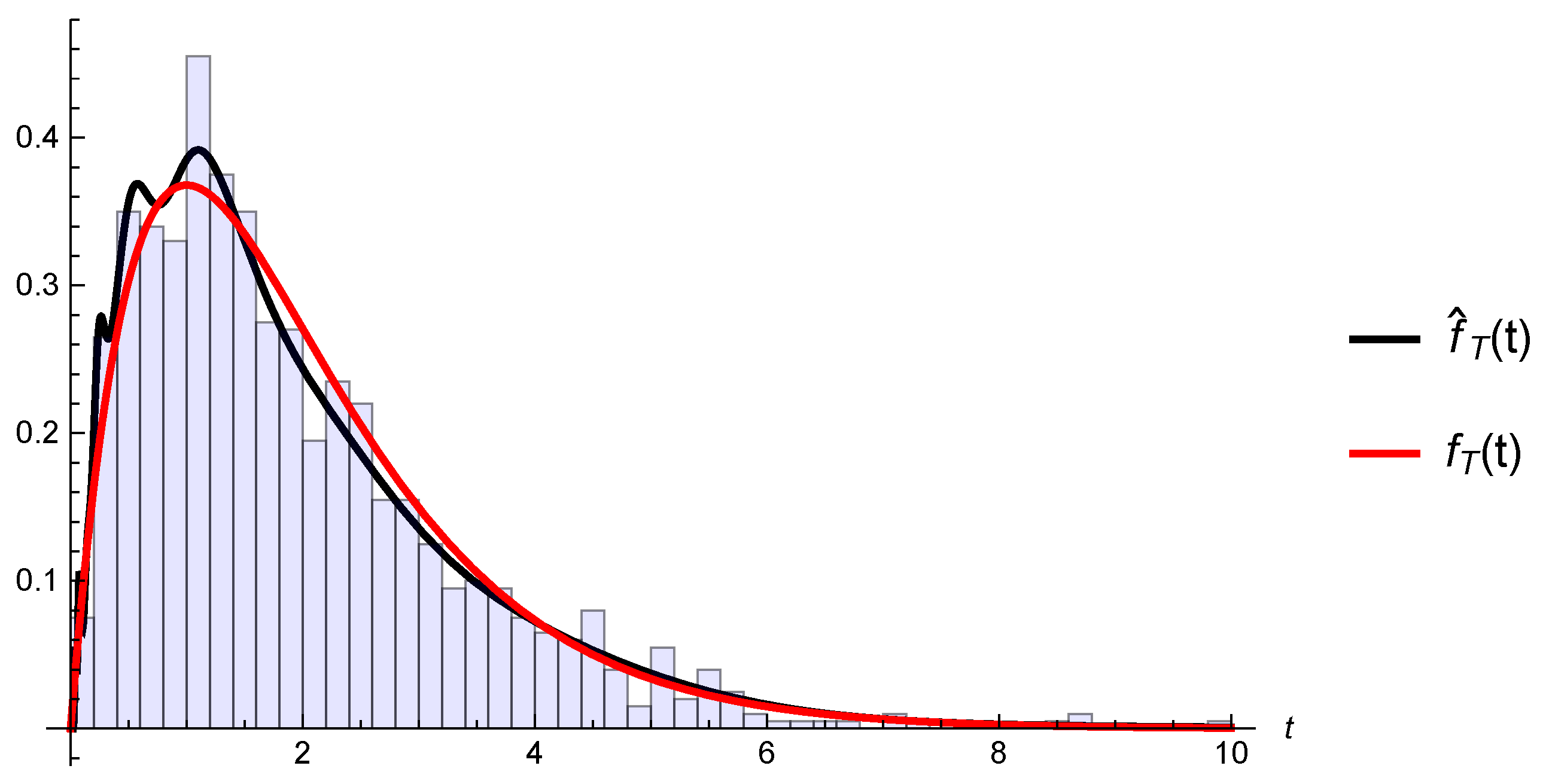
5. Statistical Complement

In this part of the manuscript we will discuss the effect of estimated parameters on the aforementioned numerical methodology for the computation of functionals of X ˜ . We place our focus on the jump intensity λ and jump size distribution F Y . Naturally, the estimators used are based on a sample { ( Y i , T i ) } i N of (iid) claims and inter-arrival times (or—practically correct—a finite sub-set is used).

5.1. Kernel Estimator

Our main goal is to compute (4), which will allow us to make a quantitative valuation of the underlying insurance line. In order to determine the function (4) according to the specifics of a given insurance line, we have to use statistical methods to incorporate the behavior of important characteristics; i.e., the distribution of the inter-arrival time F T and the distribution of the claim height F Y .
For this purpose we apply a non-parametric approach; namely, we use the kernel method to estimate the respective densities f T and f Y . This is necessary, since we want to apply our approximation procedure for the construction of PDMPs later. Therefore, we need to have smooth estimates for these densities and for the associated jump rate λ ( t ) = f T ( t ) t f T ( s ) d s in particular.
Given the respective data we use the kernel method—after a logarithmic transformation of it, as described in the monograph Silverman (1986, p. 30))—to estimate the required probability densities. The approach works as follows: since we want to estimate densities with support on the positive half line, we take the logarithms of the data and apply the common kernel estimator for the transformed data to obtain a function f ^ l o g ( z ) , where we denote the given data points by data 1 , data ν , the sample size by ν , the bandwidth by h and the kernel by K. We obtain that
f ^ l o g ( z ) = 1 ν h i = 1 ν K z l o g ( data i ) h .
The estimator of the actual data is then given by f ^ ( z ) = 1 z f ^ l o g ( l o g ( z ) ) for z > 0 . For our numerical considerations we use Wolfram Mathematica, which in turn uses for the density at point z a linearly interpolated version of the kernel estimator 1 ν h i = 1 ν K z data i h . Added to this, the used kernel K is the density of the standard normal distribution and in order to determine the bandwidth h, the Silverman rule is applied. Note that it is mentioned in Silverman (1986, p. 45 et seqq.) that using this rule for the bandwidth can lead to overly smooth results, if the underlying distribution is multimodal.

5.2. Uniform Consistency

Of course we have to make sure that an increase of the number ν of sample points will lead to a decrease of the estimation error. Following again the lines of Silverman (1986, pp. 71–74) we obtain that
sup x | f ^ ( x ) f ( x ) | 0 as ν
with probability one; if the kernel K is bounded, or has a bounded variation, it holds that | K ( t ) | d t < and K ( t ) d t = 1 , in addition to the property that the set of discontinuities of K is a Lebesgue null set. Furthermore, the true density f has to be uniformly continuous on ( , ) and the bandwidth has to fulfill h ν 0 and ν h ν log ( ν ) as ν .
Fulfilling the above assumptions ensures that the estimators of the density converge uniformly against the true density. In order to make sure that we can apply Theorem 5.16 from Kritzer et al. (2019) we have to estimate the jump rate λ ( t ) for F T ( t ) < 1 in such a way that the estimator converges uniformly. With regard to the special form of λ ( t ) = f T ( t ) 1 F T ( t ) we consider the estimation on a compact interval; compare to (Liu and Van Ryzin 1985, p. 600, Thm. 3.4).
For that purpose, we choose an analogous starting point as in Antoniadis et al. (1999, p. 600, pp. 65–66). First of all, we set Θ F T = sup { t : F T ( t ) < 1 } and restrict our estimation procedure to the finite interval [ 0 , Θ ¯ ] , where Θ ¯ < Θ F T holds. Let now F ^ T ν be the empirical distribution function of T using ν data points; we obtain with Θ F ^ T ν = sup { t : F ^ T ν ( t ) < 1 } that Θ F ^ T ν = T ( ν ) . Here T ( ν ) denotes the ν th order statistic of a sequence of length ν , and thus, the largest element. In the implementation of the statistical procedure one can take Θ ¯ = T ( ν ) , since it can be shown that Θ F ^ T ν = T ( ν ) Θ F T almost surely if ν . The uniform convergence of the jump rate estimator can then be verified analogously as described in Liu and Van Ryzin (1985). For further results on uniform consistency, see for example, Einmahl and Mason (2005).
Remark 4.
Note that the above requirements for uniform convergence are fulfilled using for example the Gaussian kernel in combination with the Silverman rule, which yields a bandwidth proportional to ν 1 5 .

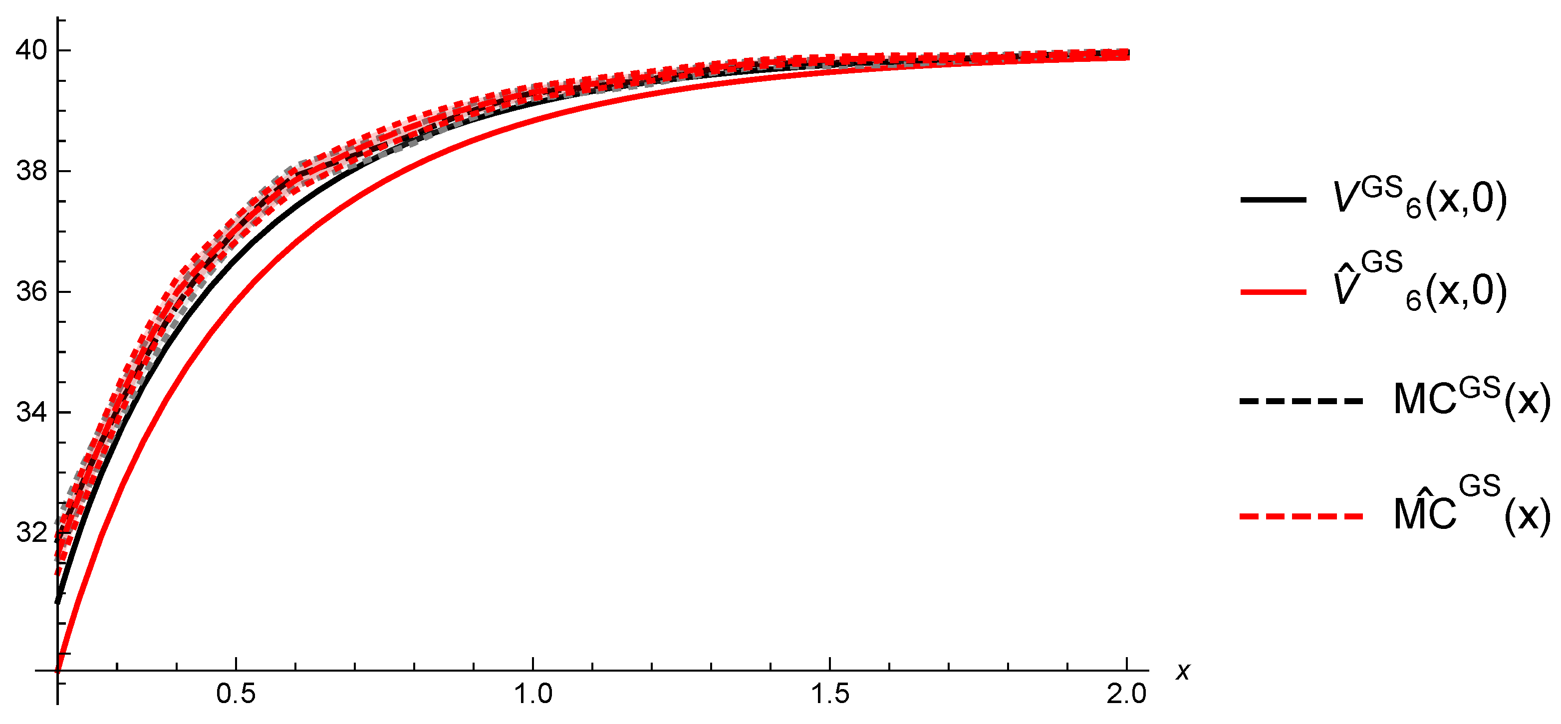
5.3. Convergence of Estimated Gerber-Shiu Functions

Complementing the discussion about the convergence above, we now investigate the respective behaviors of the generator A ^ h when we replace λ , F Y and c by their estimated counterparts λ ^ , F ^ Y and c ^ in A h . Note that concerning the estimation of the function c we demand that the respective estimator c ^ has to converge uniformly to the true c. In our numerical examples we try to mirror real-life applications. This leads to the fact that the premium rate c underlies the estimation procedure in such a way that it depends on the first moments of Y and T. Hence, we assume that c = E [ Y ] E [ T ] ( 1 0 . 1 ) , which is a quite standard approach. Another established option for a common premium principle would be the variance premium principle.
We can directly tie in with the line of arguments provided in Section 4.3. This will yield the convergence of our computational procedure. Hence, let again E h = { k h : k Z } × R 0 + E denote the state space of the associated Markov chain. For the starting value X 0 h = k x ( h ) h , where k x ( h ) : = x h we have that X 0 h X 0 if h 0 as above. Here h again denotes the step size of the discretization, and moreover, ν denotes the sample size. Finally, let f C b ( E , R ) ; then, we have to show that the following difference tends to zero:
A f ( x , t ) A ^ h f ( k x ( h ) h , t ) A f ( x , t ) A h f ( k x ( h ) h , t ) + A h f ( k x ( h ) h , t ) A ^ h f ( k x ( h ) h , t ) .
Since we know from Section 4.3 that the first summand tends to zero uniformly in ( x , t ) , the same remains to be shown for the second one. Hence, we obtain for the second term
A h f ( k x ( h ) h , t ) A ^ h f ( k x ( h ) h , t ) λ ( t ) l = k x ( h ) 1 f ( l h , 0 ) p k x ( h ) l h λ ^ ( t ) l = k x ( h ) 1 f ( l h , 0 ) p ^ k x ( h ) l h + λ ( t ) λ ^ ( t ) f ( k x ( h ) h , t ) + c ( k x ( h ) h ) c ^ ( k x ( h ) h ) f ( ( k x ( h ) + 1 ) h , t ) f ( k x ( h ) h , t ) h λ ( t ) λ ^ ( t ) l = k x ( h ) 1 f ( l h , 0 ) p k x ( h ) l h + λ ^ ( t ) l = k x ( h ) 1 f ( l h , 0 ) p k x ( h ) l h l = k x ( h ) 1 f ( l h , 0 ) p ^ k x ( h ) l h + λ ( t ) λ ^ ( t ) f + c ( k x ( h ) h ) c ^ ( k x ( h ) h ) f x .
In fact, the above terms tend to zero uniformly in ( x , t ) on compacts for t a.s., because of the aforementioned convergence of the estimators λ ^ , F ^ Y and c ^ as ν .
Note that we use the following estimate for the series term
l = k x ( h ) 1 f ( l h , 0 ) p k x ( h ) l h l = k x ( h ) 1 f ( l h , 0 ) p ^ k x ( h ) l h 2 K f F Y F ^ Y + f F ¯ Y ( K ) + F ¯ ^ Y ( K ) ,
where K has to be chosen such that max F ¯ Y ( K ) , F ¯ ^ Y ( K ) < ε 2 f for a given ε > 0 .
Overall, if we take the limits h 0 and ν , then we obtain that the left-hand side of (9) converges a.s. to zero uniformly on compacts in t and uniformly in x.
Remark 5.
In order to meet the requirements of the above statistical procedure, we denote with ( Θ N , G N , P ) the sample space such that for ω Θ N we have that { Y i ( ω ) , T i ( ω ) } i N denotes one sample. Given such an ω Θ N and a sample size ν N we have that c ^ = c ^ ( ω , ν ) , λ ^ = λ ^ ( ω , ν ) and F ^ Y = F ^ Y ( ω , ν ) . Note that the dependence on ν expresses that the estimators only use the first ν claim heights and inter-arrival times, respectively, for the estimation. Hence, following the previous lines, this yields that N G N with P ( N ) = 0 such that ω Θ N N
c ^ ( ω , ν ) cuniformly,
λ ^ ( ω , ν ) λ uniformly on compacts in t and
F ^ Y ( ω , ν ) F Y uniformly
for ν . Furthermore, for each ω Θ N N we have that
A ^ ( ω , ν ) f = t f ( x , t ) + c ^ ( x , ω , ν ) x f ( x , t ) λ ^ ( t , ω , ν ) f ( x , t ) + λ ^ ( t , ω , ν ) 0 f ( x y , 0 ) d F ^ Y ( y , ω , ν )
is generator of a sequence of PDMPs on E with index ν N . These converge as ν to A f uniformly in ( x , t ) on compacts for t . Notice that incorporating the statistical procedure we use G 0 = σ ( { ( Y i , T i ) : i N } ) F 0 in order to face fixed characteristics as an underlying basis of our considered renewal risk model. Above we have shown that for each such ω, and the discrete version of A ^ , A ^ h converges in the appropriate sense to A .
At this point we are again in the situation to use Kritzer et al. (2019, Theorem 5.16), which yields a.s. weak convergence of the approximated and estimated process against its underlying counterpart.

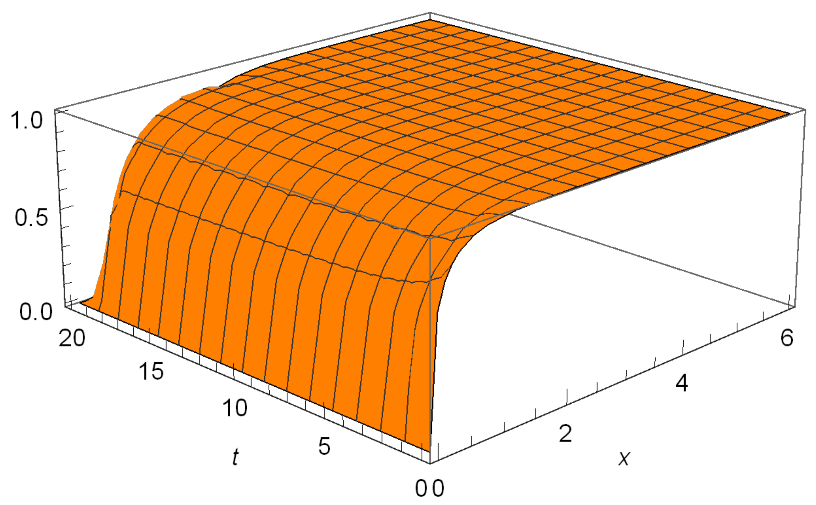
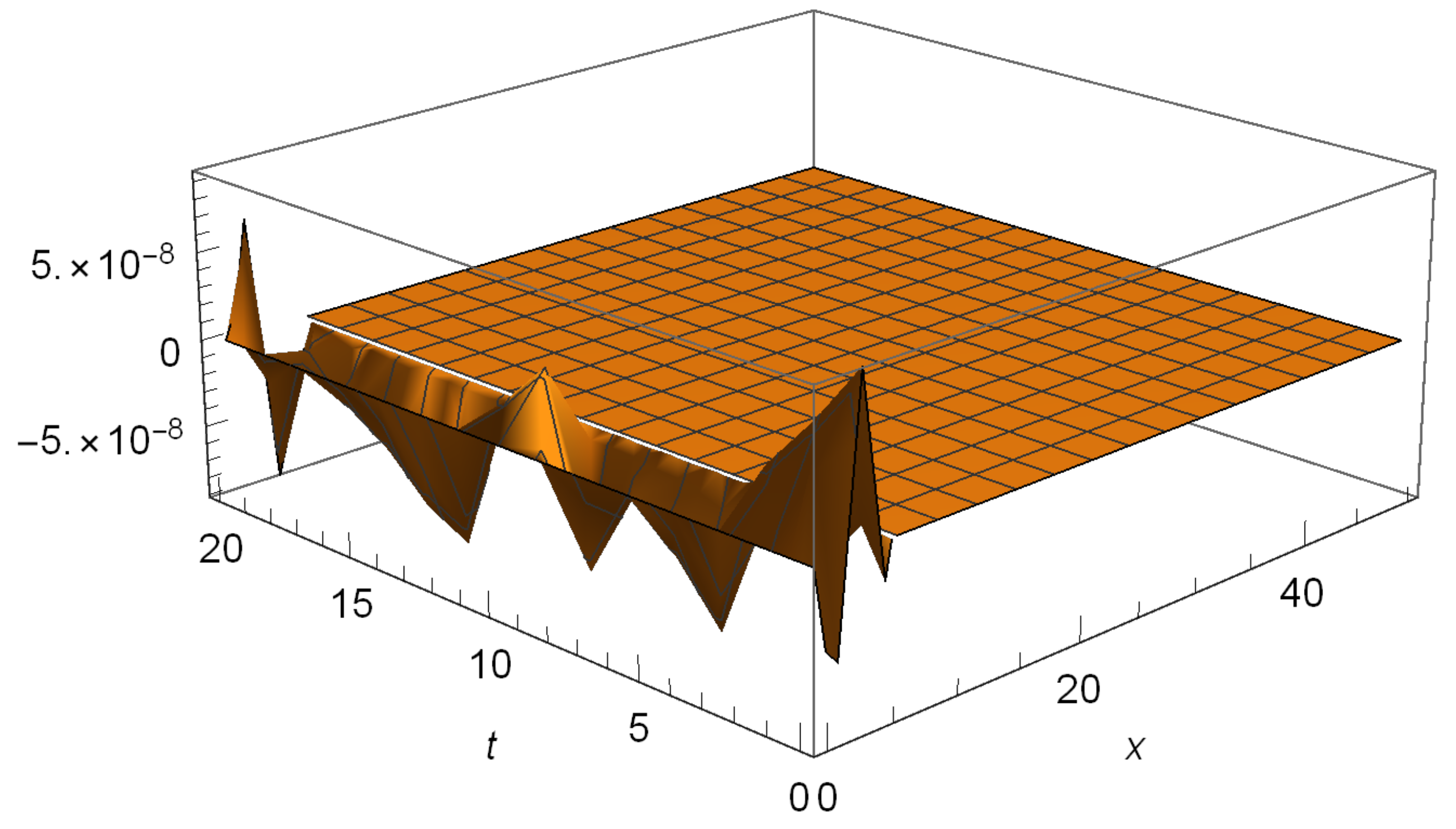
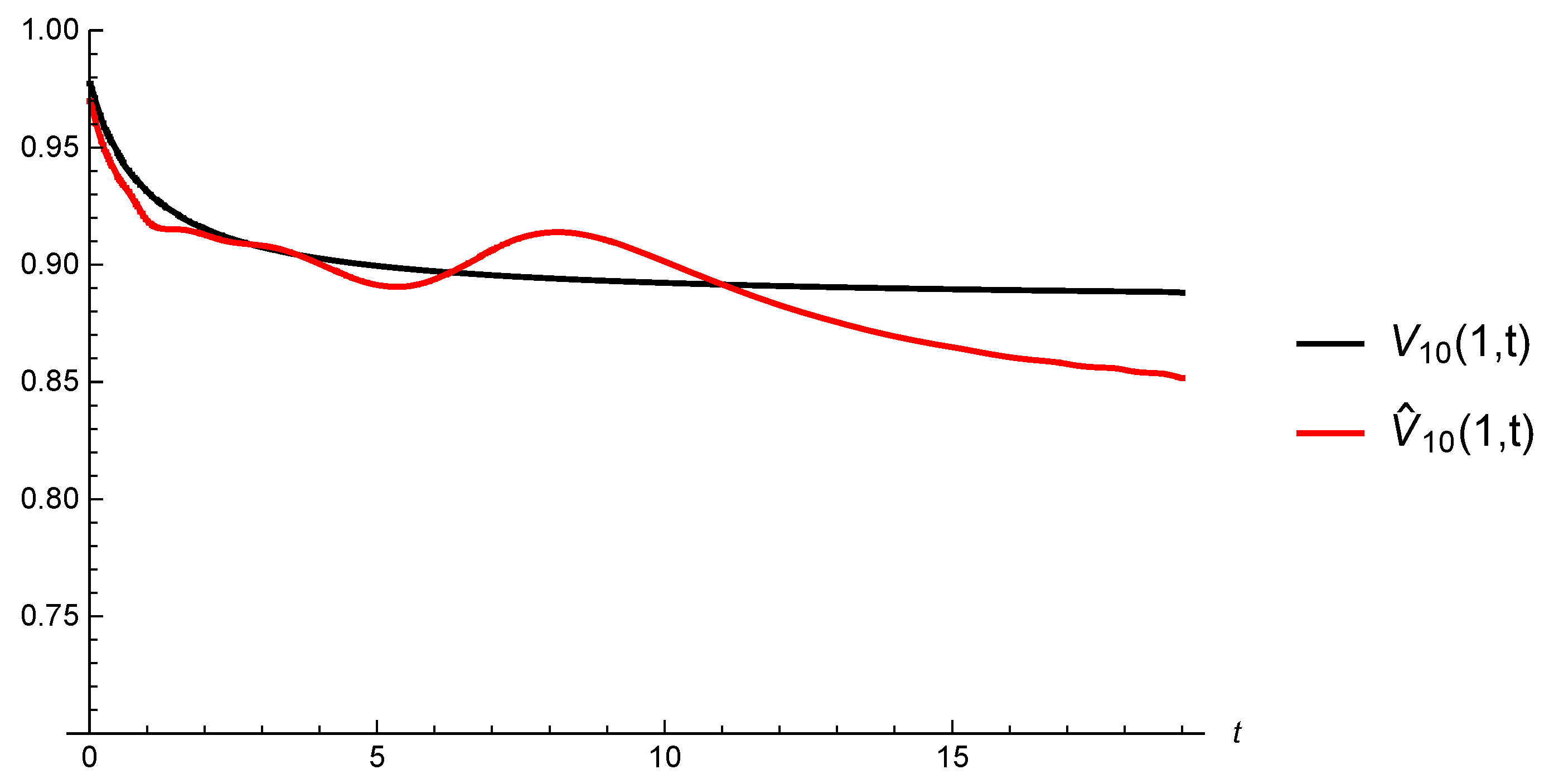
6. Numerical Illustrations

Complementing the theoretical part, we illustrate in the subsequent paragraphs numerical results for the two considered problems. In order to outline the exemplifications we want to point out that there are four different approaches which result in four functions V ( x , t ) , V ^ ( x , t ) , M C ( x ) and M C ^ ( x ) . First of all V ( x , t ) denotes the solution we obtain following the lines in Section 4. On the other hand, if we replace in this setup the respective characteristics by their estimated counterparts we end up with the solution V ^ ( x , t ) . Furthermore, we computed via Monte-Carlo simulations the functions M C ( x ) and M C ^ ( x ) where we fixed t = 0 , and for the latter we again made use of the estimated ingredients. The simulated results are primarily needed for reasons of comparability and hence serve as a benchmark.

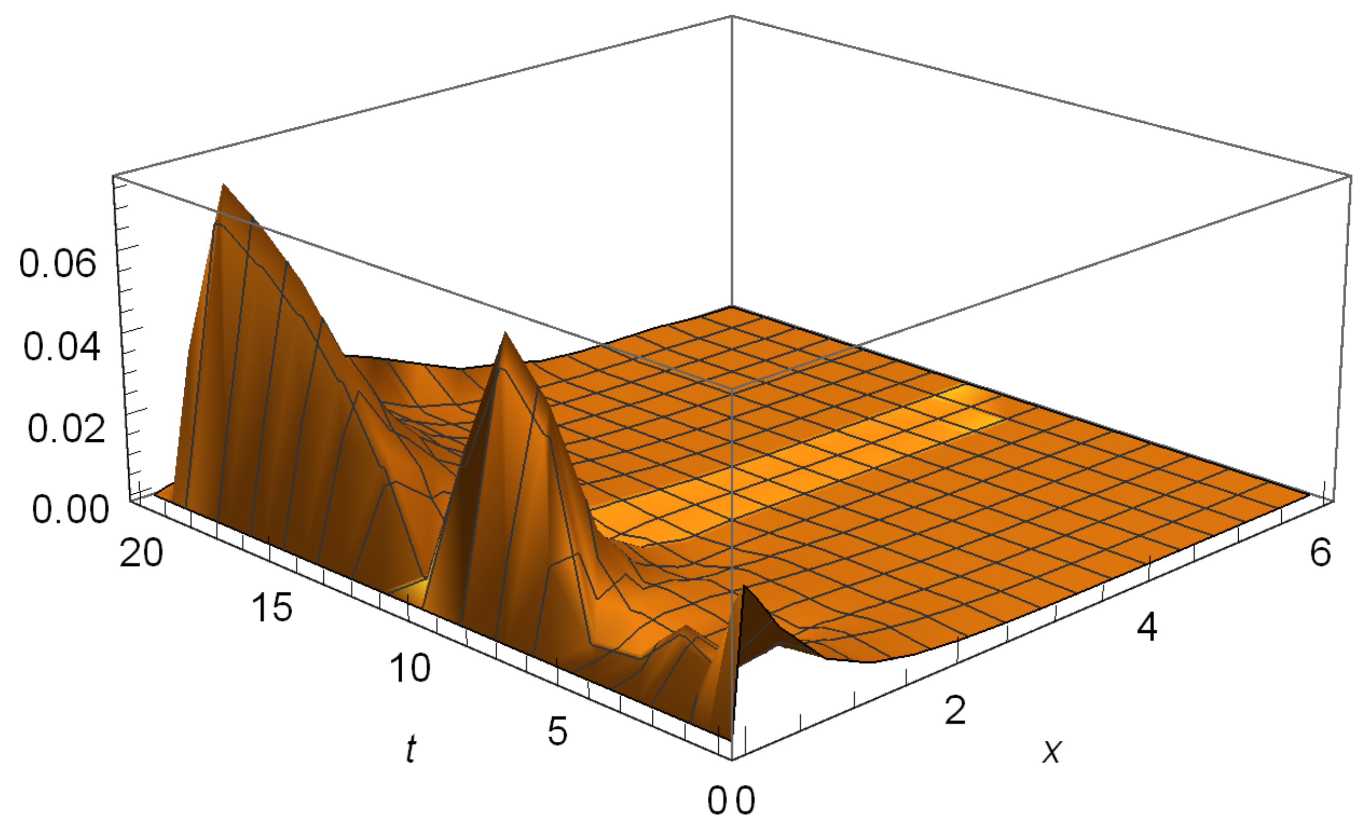
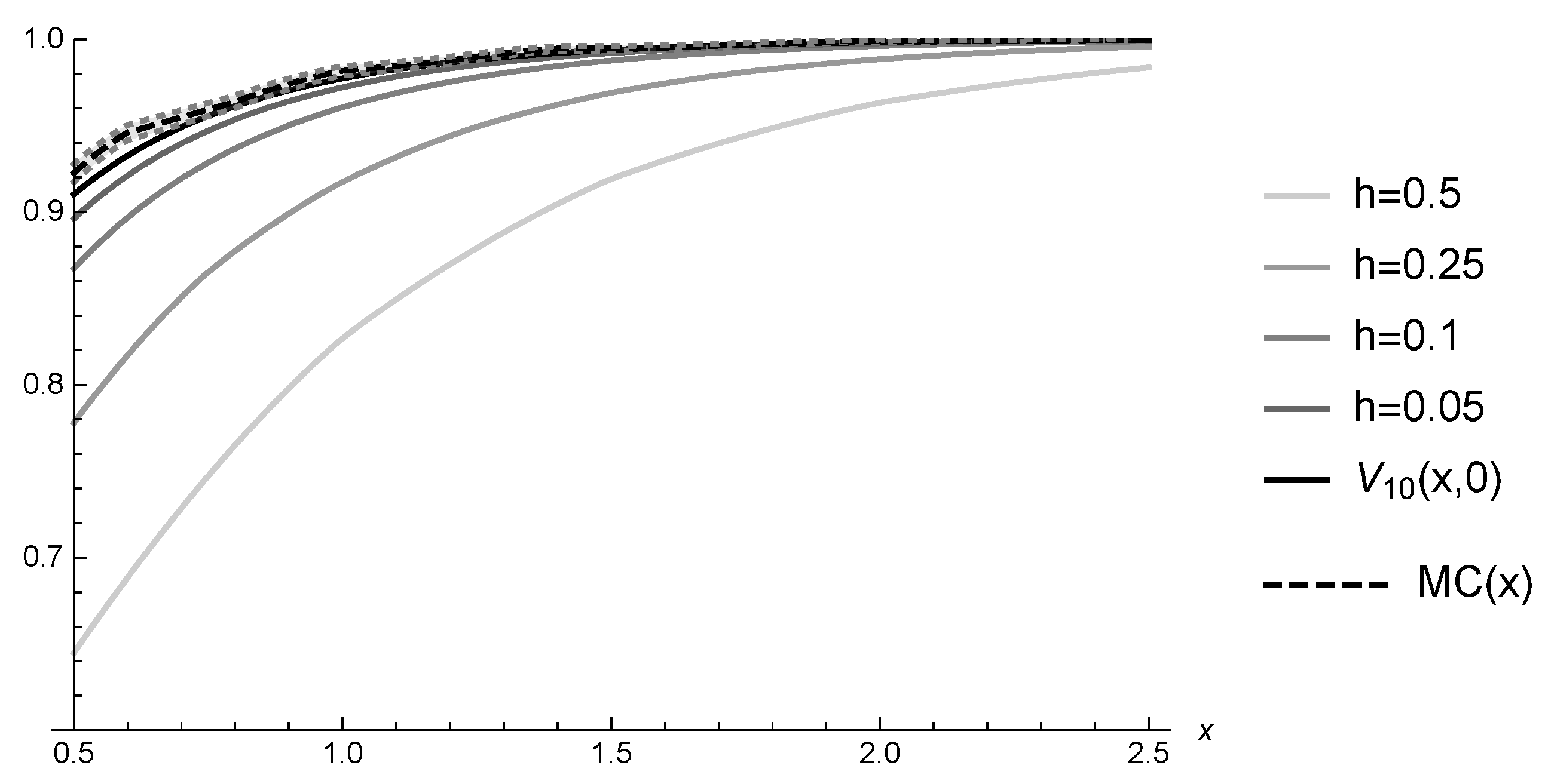
6.1. Hitting Probabilities

In the following graphical illustrations we have applied the above described approach to compute the hitting probability, here denoted by V ( x , t ) . Note that the cut-off value a is natural for our choice of non-constant drift c ( x ) for which ruin is certain. In the general situation—constant c or unbounded ODE paths—the probability of hitting a finite level a before getting ruined serves as an approximation for the ruin probability. Certainly, as a we would face a rare event problem. In such a situation, one needs to fix an appropriate finite a. This is in order to not lose the focus of the method, since otherwise there would be need to consider variance reduction methods or the like for dealing with this additional feature.
We have used the set of parameters listed in Table 1.
Furthermore, as mentioned above we assumed that c ( x ) = κ ( b 1 x ) ( x a 1 ) I { a 1 < x < b 1 } . A probabilistic reference solution is based on Monte Carlo simulation, where we used 10000 sample paths of the renewal process, where we used 2000 random points in turn for every path to simulate the inter-arrival time and the claim height, respectively; i.e., 1000 jump events. The solution after the 10th jump iteration is shown in Figure 1. Moreover, the associated improvement, namely, the difference of the last two iterations illustrated in the subsequent Figure 2, is already relatively small.
Figure 3 depicts this hitting probability for x = 1 as a function in t. The black curve V 10 ( 1 , t ) corresponds to the numerical solution using the above mentioned distribution functions, and the red curve V ^ 10 ( 1 , t ) depicts the solution we obtain using their estimated counterparts with ν = 1000 given data points generated from the respective distribution. What we immediately observe is that the accuracy of the latter method depends to an enormous extent on the quality of the estimator for the hazard rate. This is explained by the fact that the ODE methods rely on smooth coefficients with preferably low variation. In our approach we need to estimate the density f T in such a manner that the associated hazard rate function is sufficiently regular; see Figure 4.
This is for the applicability of the above mentioned theoretical results. Using smooth kernel estimators for the density leads to an appropriate estimator of the hazard rate—from an analytic point of view. Nevertheless, the hazard’s estimation error explains the deviation of V 10 ( x , t ) and V ^ 10 ( x , t ) for large t values. This is an immediate consequence of our way of computing the desired quantities. The difference of V 10 ( x , t ) and V ^ 10 ( x , t ) as a function of x and t is shown in Figure 5. One can see clearly that for increasing x the hazard’s impact declines.
The convergence regarding the discretization method described above is illustrated in Figure 6, where we can see a sequence of solutions for decreasing step size h. The use of a step size h = 0 . 025 applied for the computation of V 10 ( x , 0 ) results in a solution which is reasonably close to the one obtained via a comparative MC-simulation (depicted as a dashed line together with its 95% confidence intervals).
In order to illustrate the development concerning the estimation as ν increases, we list in Table 2 the values of the function V 10 ( x , t ) and V ^ 10 ( x , t ) for t = 0 and different values of x, in addition to the results from the MC-simulation.

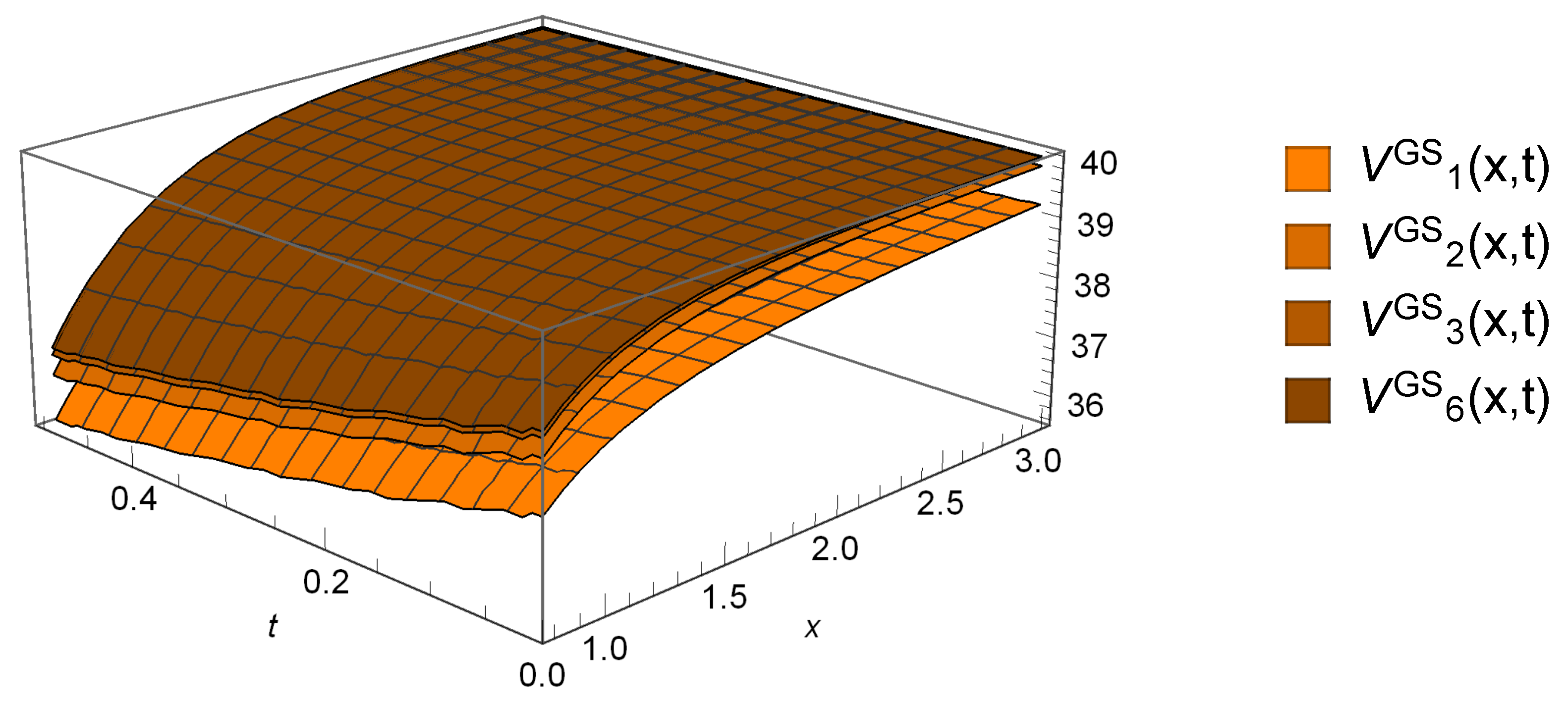
6.2. Gerber-Shiu Functions

As above, we provide some illustrations of the numerical computations concerning the determination of the expectation (4) in this passage in a more general setting. We denote the solution in this framework by V G S ( x , t ) . We have made the following assumptions and used the parameters given in Table 3.
Moreover, we have again c ( x ) = κ ( b 1 x ) ( x a 1 ) I { a 1 < x < b 1 } . In Table 4 we display values obtained using the four different approaches described above for t = 0 and for several values of x. An immediate observation is that the deviation declines while x increases, which is due to the decreasing influences of the errors of estimation affecting the coefficients and the boundary conditions.
Figure 7 illustrates the improvement of the solution of the GS function for different n.
Figure 8 shows the solution for the GS function compared to the version obtained using the estimated parameters. In addition, the result of the MC-simulation and the respective confidence intervals for both of the computations are included. Note that for the computation of the MC-simulated counterpart M C G S ( x ) of V G S ( x , 0 ) , we have used the true distributions F T and F Y , whereas for the quantity M C ^ G S ( x ) we generated the sample points from the estimated distributions given ν = 1000 data points each. In fact this corresponds to a bootstrap procedure. We can observe that the simulated results are not very sensitive with respect to estimation, which can also be seen in Table 4 and that the numerically calculated V G S ( x , 0 ) , with a grid size of h = 0 . 025 , lies partly within the 95% confidence band. In contrast to this, the numerically determined V G S ( x , 0 ) , with estimated coefficients, is not able to reach the confidence band. This is because of the fact that the approximation error of the estimated hazard rate is too significant here—even for a relatively large sample size of ν = 1000 . This nicely illustrates that the stated convergence results have a qualitative nature and hold asymptotically for ν and h 0 . At the same time one observes that this initial error becomes less influential for increasing x.

7. Conclusions and Discussions

In this contribution we present numerical and statistical methods for the computation of Gerber-Shiu functions in general renewal risk models. The numerical method we provide incorporates the fact that the underlying model itself faces stochastic ingredients, i.e., drift, estimated intensity and distribution of claims, and thus takes the statistical aspect into account. In particular, we have shown that the proposed schemata converge and illustrate these findings by means of two informative examples. For practical applications we wish to point out that the solutions obtained via MC methods are relatively robust with respect to estimation, whereas by nature of the scheme, methods from numerical analysis are more sensitive. The main reason is typically the high variation of the estimated hazard rate. Here, the fact that estimating derivatives is a relatively complex task impacts on our approach. On the other hand, the computations are less affected by estimation of the claims’ distribution F Y .
Several directions are open for future research. Namely, the incorporation of estimation methods such as the use of parametrized families or the direct usage of phase-type approximations for the empirical distribution functions of observed inter-jump times and claims.

Author Contributions

J.A.S. and S.T. contributed equally to this work. Both authors have read and agreed to the published version of the manuscript.

Funding

This research received no external funding.

Acknowledgments

The authors would like to thank the anonymous referees for their remarks which clearly helped to improve this contribution.

Conflicts of Interest

The authors declare no conflict of interest.

References

  1. Albrecher, Hansjörg, and Eleni Vatamidou. 2019. Ruin Probability Approximations in Sparre Andersen Models with Completely Monotone Claims. Risks 7: 104. [Google Scholar] [CrossRef] [Green Version]
  2. Alvarez, Luis, and Larry Shepp. 1998. Optimal harvesting of stochastically fluctuating populations. Journal of Mathematical Biology 37: 155–77. [Google Scholar] [CrossRef]
  3. Antoniadis, Anestis, Gérard Grégoire, and Guy Nason. 1999. Density and hazard rate estimation for right-censored data by using wavelet methods. Journal of the Royal Statistical Society: Series B (Statistical Methodology) 61: 63–84. [Google Scholar] [CrossRef]
  4. Asmussen, Søren, and Hansjörg Albrecher. 2010. Ruin Probabilities, 2nd ed. River Edge: World Scientific. [Google Scholar]
  5. Asmussen, Søren, Olle Nerman, and Marita Olsson. 1996. Fitting phase-type distributions via the em algorithm. Scandinavian Journal of Statistics 23: 419–41. [Google Scholar]
  6. Azaïs, Romain, François Dufour, and Anne Gégout-Petit. 2014. Non-parametric estimation of the conditional distribution of the interjumping times for piecewise-deterministic Markov processes. Scandinavian Journal of Statistics 41: 950–69. [Google Scholar] [CrossRef] [Green Version]
  7. Azaïs, Romain, François Dufour, and Anne Gégout-Petit. 2013. Non-parametric estimation of the jump rate for non-homogeneous marked renewal processes. Annales de l’IHP Probabilités et Statistiques 49: 1204–31. [Google Scholar] [CrossRef] [Green Version]
  8. Brémaud, Pierre. 1981. Point Processes and Queues. New York and Berlin: Springer. [Google Scholar]
  9. Davis, Mark. 1993. Markov Models and Optimization. London: Chapman & Hall. [Google Scholar]
  10. Einmahl, Uwe, and David Mason. 2005. Uniform in bandwidth consistency of kernel-type function estimators. The Annals of Statistics 33: 1380–403. [Google Scholar] [CrossRef] [Green Version]
  11. Fleming, Wendell Helms, and Halil Mete Soner. 1993. Controlled Markov Processes and Viscosity Solutions. New York: Springer. [Google Scholar]
  12. Gerber, Hans-Ulrich, and Elias Shiu. 1998. On the time value of ruin. North American Actuarial Journal 2: 48–78. [Google Scholar] [CrossRef]
  13. Gerber, Hans-Ulrich, and Elias Shiu. 2005. The time value of ruin in a Sparre Andersen model. North American Actuarial Journal 9: 49–84. [Google Scholar] [CrossRef]
  14. Kallenberg, Olav. 2002. Foundations of Modern Probability. (Probability and its Applications), 2nd ed. New York: Springer. [Google Scholar]
  15. Kritzer, Peter, Gunther Leobacher, Michaela Szölgyenyi, and Stefan Thonhauser. 2019. Approximation methods for piecewise deterministic Markov processes and their costs. Scandinavian Actuarial Journal 2019: 308–35. [Google Scholar] [CrossRef] [PubMed] [Green Version]
  16. Kushner, Harold, and Paul Dupuis. 2001. Numerical Methods for Stochastic Control Problems in Continuous Time, 2nd ed. New York: Springer. [Google Scholar]
  17. Liu, Regina, and John Van Ryzin. 1985. A histogram estimator of the hazard rate with censored data. The Annals of Statistics 13: 592–605. [Google Scholar] [CrossRef]
  18. Preischl, Michael, Stefan Thonhauser, and Robert Tichy. 2018. Integral equations, quasi-Monte Carlo methods and risk modeling. In Contemporary Computational Mathematics—A Celebration of the 80th birthday of Ian Sloan. Cham: Springer, pp. 1051–74. [Google Scholar]
  19. Rolski, Tomasz, Hanspeter Schmidli, Volker Schmidt, and Jozef Teugels. 1999. Stochastic Processes for Insurance and Finance. New York: John Wiley & Sons. [Google Scholar]
  20. Schmidli, Hanspeter. 2017. Risk Theory. Cham: Springer. [Google Scholar]
  21. Shimizu, Yasutaka. 2012. Non-parametric estimation of the Gerber-Shiu function for the Wiener-Poisson risk model. Scandinavian Actuarial Journal, 56–69. [Google Scholar] [CrossRef]
  22. Shimizu, Yasutaka, and Zhimin Zhang. 2017. Estimating Gerber-Shiu functions from discretely observed Lévy driven surplus. Insurance: Mathematics and Economics 74: 84–98. [Google Scholar] [CrossRef]
  23. Silverman, Bernard Walter. 1986. Density Estimation for Statistics and Data Analysis. London: Chapman & Hall, Monographs on Statistics and Applied Probability. [Google Scholar]
  24. Sparre Andersen, Erik. 1957. On the collective theory of risk in the case of contagion between the claims. Bulletin of the Institute of Mathematics and its Applications 2: 212–19. [Google Scholar]
  25. Vatamidou, Eleni, Ivo Jean Baptiste François Adan, Maria Vlasiou, and Bert Zwart. 2013. Corrected phase-type approximations of heavy-tailed risk models using perturbation analysis. Insurance: Mathematics and Economics 53: 366–78. [Google Scholar] [CrossRef] [Green Version]
  26. Vatamidou, Eleni, Ivo Jean Baptiste François Adan, Maria Vlasiou, and Bert Zwart. 2014. On the accuracy of phase-type approximations of heavy-tailed risk models. Scandinavian Actuarial Journal 2014: 510–34. [Google Scholar] [CrossRef] [Green Version]
Figure 1. Hitting probability as a function of ( x , t ) .
Risks 08 00024 g001
Figure 2. Difference of 9th and 10th iterations.
Risks 08 00024 g002
Figure 3. The hitting probabilities in x = 1 —original and estimated.
Risks 08 00024 g003
Figure 4. Comparison of the jump time density and its estimated analogue together with the used data depicted in a histogram.
Risks 08 00024 g004
Figure 5. Difference of V 10 ( x , t ) and V ^ 10 ( x , t ) .
Risks 08 00024 g005
Figure 6. Improvement of the solution due to decrease of step size h.
Risks 08 00024 g006
Figure 7. Sequence of solutions for n = 1 , 2 , 3 , 6 .
Risks 08 00024 g007
Figure 8. Comparison of solution with and without estimation together with their MC simulated counterparts.
Risks 08 00024 g008
Table 1. Set of parameters used in the first example.
κ a 1 b 1 hanYT ν t end
0.2 010 0.025 610 Γ ( 3 , 3 ) Γ ( 2 , 1 ) 100020
Table 2. Development of the solution with estimation due to variation of the sample size ν .
x = 0.5x = 1x = 1.5x = 2x = 2.5
M C ( x ) 0.92260.98170.99460.99910.9997
M C ^ ( x ) 0.92280.98200.99610.99910.9998
V 10 ( x , 0 ) 0.91020.97730.99380.99820.9995
V ^ 10 ν = 1000 ( x , 0 ) 0.89170.96980.99070.99690.9989
V ^ 10 ν = 750 ( x , 0 ) 0.89610.97120.99170.99770.9994
V ^ 10 ν = 500 ( x , 0 ) 0.90010.97330.99250.99800.9995
V ^ 10 ν = 250 ( x , 0 ) 0.90360.97320.99150.99720.9991
V ^ 10 ν = 50 ( x , 0 ) 0.91590.97780.99290.99820.9997
V ^ 10 ν = 25 ( x , 0 ) 0.87010.96200.98840.99730.9994
Table 3. Set of parameters used in the second example.
κ a 1 b 1 l ( x ) δ ψ ( x , z ) β hanYT ν t end
0.2 0102 0.05 e β z 2 0.025 96 Γ ( 3 , 3 ) Γ ( 2 , 1 ) 100020
Table 4. Comparison of results obtained via different approaches.
x = 0.5x = 1x = 1.5x = 2x = 2.5
M C G S ( x ) 37.026739.295539.792539.965839.9869
M C ^ G S ( x ) 37.035139.307139.849439.964939.9903
V 6 G S ( x , 0 ) 36.544339.124439.759239.931739.9802
V ^ 6 G S ( x , 0 ) 35.830938.836339.641339.880839.9577

