Macroeconomic News Sentiment: Enhanced Risk Assessment for Sovereign Bonds

Abstract

We enhance the modelling and risk assessment of sovereign bond spreads by taking into account quantitative information gained from macro-economic news sentiment. We investigate sovereign bonds spreads of five European countries and improve the prediction of spread changes by incorporating news sentiment from relevant entities and macro-economic topics. In particular, we create daily news sentiment series from sentiment scores as well as positive and negative news volume and investigate their effects on yield spreads and spread volatility. We conduct a correlation and rolling correlation analysis between sovereign bond spreads and accumulated sentiment series and analyse changing correlation patterns over time. Market regimes are detected through correlation series and the impact of news sentiment on sovereign bonds in different market circumstances is investigated. We find best-suited external variables for forecasts in an ARIMAX model set-up. Error measures for forecasts of spread changes and volatility proxies are improved when sentiment is considered. These findings are then utilised to monitor sovereign bonds from European countries and detect changing risks through time.

1. Introduction

In the wake of the sovereign debt crisis in Europe, managing and monitoring credit risk arising from sovereign bonds are increasingly important. European countries have undergone changes in terms of their financial stability, and credit spreads have widened due to increased financial risk. Modelling of sovereign bond spreads is often linked to various macroeconomic factors such as the countries’ GDP growth rate or inflation. These macroeconomic factors are monitored via scheduled announcements from official bodies e.g., treasuries and national banks but are also covered in news articles and unscheduled announcements. Changes in country dynamics and risks are reported and captured in news, which are classified as “macroeconomic news”, and can be closely monitored and quantified through news sentiment analysis.

News sentiment for equities and in particular its use in equity trading have been widely covered in various studies over the last years. An overview of equity modelling and predictability enhancements through news sentiment is given in Reference (Mitra and Mitra 2011). The dynamics of asset prices, in particular their volatility, is clearly affected by news events. These events are classified and quantified, and news sentiment can be utilised to enhance volatility prediction (see, e.g., (Mitra et al. 2009)). Sentiment Analysis is further used to improve trading decisions in equity markets. Firm-specific news sentiment affects the predicted asset return distribution; taking into consideration sentiment values increases the accuracy of a forecast and contributes to improved portfolio decisions as discussed in (Leinweber and Sisk 2011; Mitra et al. 2018), amongst others. In the Fixed Income market, however, news sentiment and its potential influence to bond spreads have just recently become more relevant in the light of electronification of bond trading (Bech et al. 2016) and sentiment lacks thorough investigation in this market. Especially macroeconomic news sentiment for sovereign bond spreads but also firm-specific news sentiment for corporate bond spreads can add value to both monitoring and forecasting of bonds. In this paper, we aim to fill this current gap and provide an extensive study on effects of news sentiment to bond spread predictions. In particular, we investigate the influence of macroeconomic news sentiment on bond spreads and develop a method to improve prediction and monitoring of sovereign bonds.

When analyzing bond spreads of European countries, various studies (e.g., (Bernoth and Erdogan 2012; Caggiano and Greco 2012; Maltritz 2012)) found influencing international and country-specific risk factors such as government debt and characterised market dynamics such as liquidity issues and fiscal policies to effect bond spreads. Economic fundamentals are seen as drivers for sovereign spreads (see (Dewachter et al. 2015)); they have been utilised to explain yield spread movements and a significant effect has been found. Following a study by (Afonso et al. 2015), factors that influence sovereign spreads in Europe are time varying. The authors highlight the fact that financial determinants have changing effects on spreads, but that their influence is increasing in times of crisis. A further investigation of time-varying factors can be done by considering macroeconomic news, which reports on changing dynamics and influences from issuing and neighbouring countries. News and sentiments for sovereign bond spreads were investigated by (Beetsma et al. 2013; Mohl and Sondermann 2013), amongst others. They investigated the influence of news announcements on spreads during the European debt crisis and found evidence that information from government statements as well as news from a European newsflash platform influenced yield spreads both nationally but also across countries, pointing to spill-over effects in the debt crisis.

Our paper contributes to the current literature an in-depth analysis of the impact of processed macroeconomic news and its sentiment towards European sovereign yield spreads. In particular, we investigate the dynamics of daily sovereign spread changes and find a relation between their daily forecasts and news sentiment time series. Our findings show that the forecast of yield spreads can be enhanced when daily news sentiment is taken into account. News is split into positive and negative news items, their influences are investigated separately as well as jointly in a multivariate Integrated Autoregressive Moving Average with explanatory variables (ARIMAX) model. We study various combinations of external variables and give details and results of five model settings, which produce the best forecast outcome. The ARIMAX model gives daily one-step ahead predictions of spread changes and volatility proxies. The in-depth analysis of ARIMAX performance and its improvements through external news variables leads us to propose the enhancement of sovereign bond analysis through including significant news time-series for five European markets.

2. Materials and Methods

2.1. Bond Data

In order to establish rules to monitor risks of a bond portfolio over time, we analyse sovereign bond spreads of five European countries. We distinguish between short-term bonds with a maturity between three months and five years and long-term bonds with maturities between five and 30 years. We analyse sovereign bond data from Thomson Reuters Datascope (see (Thomson Reuters DataScope 2018) for more details; a subscription is needed; therefore, our utilised datasets cannot be made openly available) and calculate spreads between the bond yields and the AAA-rated bond yield quoted from the European Central Bank (ECB). The spread series which we model is obtained as a spread referring to ECB AAA Svenson yields, see Svensson (1994) for more details.

Our analysis covers data from five European countries, namely Germany, Great Britain, Italy, Spain and France. For each country, we consider both short-term and long-term bonds issued by the countries between 2007 and 2017. The chosen countries reflect the diversity of European economies in that time period. Two of the analysed countries are from the PIIGS group (Portugal, Ireland, Italy, Greece and Spain) which were in the heart of the European debt crisis and exhibited economic downturn. Great Britain and France are considered more stable economies, but both dealt with relevant economic news events such as the Brexit Referendum or controversial elections during the considered time period. Finally, we analyse bonds issued by Germany which is handled as the most risk-free economy within the group. Therefore, our choice of countries reflects various economic situations, the analysis will show how news have adverse effects in different economic settings. The analysed bond data includes more than 300 bonds, and daily closing prices from Thomson Reuters Pricing are utilised. We focus on analysing spreads of single tradeable sovereign bonds, therefore concentrating on analysing a link between macroeconomic news and fixed income products. We would like to highlight that the obtained results can be utilised by risk management models in the Fixed Income domain.

2.2. Macroeconomic News Sentiment

We wish to analyse the effect news articles and macroeconomic announcements have on spreads of bond yields. In our study, macroeconomic sentiment comprised by RavenPack is employed (see (RavenPack News Analytics 2018) for more details; a subscription is needed, therefore our utilised datasets cannot be made openly available). RavenPack News Analytics marks every macroeconomic news event in news items from various sources with a sentiment value called “ESS”—event sentiment score. This sentiment value lies between $-1$ and 1 and quantifies the sentiment of a particular news event for the chosen entity. In our case, we choose the bond issuer as the entity we would like to follow. We create daily news time series out of all sentiment values that stream in over a given day. Our work clearly distinguishes itself from other literature on sovereign bond spreads and their main determinants, since we do not take into account fiscal time series and fundamentals but rather try to analyse a connection between macro-economic news sentiment and bond spreads. One main advantage of this is that we are not limited to scheduled announcements, which are still covered in our news database, and quarterly or semi-annually releases of fundamental figures. On the contrary, news items are observed throughout the day and news sentiment signals are calculated before market closing time. By following these macro-economic news on a daily basis, we get daily macro-economic signals which can be included into daily trading decisions. Analysis on fundamentals can be an addition to our signals; however, in this work, we concentrate on daily macroeconomic news sentiment and its effect on sovereign bond spreads.

We follow macroeconomic news, which are bundled under the entities Germany, Great Britain, Italy, Spain and France, respectively, representing the issuer of the sovereign bonds. A typical macroeconomic news example from our database includes the time stamp, the relevance of the news with respect to the key word (entity) as well as the event sentiment score.

Depending on weekday and time, the news item is mapped to its relevant trading day. Weekend news are shifted to Monday and any news coming in after market closing time is shifted to the next working day. For each news item $N_i$, we have given a time stamp $timest$ which consists of the date and time of the release of the news item, $timest\left(N_i\right)=(date\left(N_i\right),time\left(N_i\right)),$ where $i=1,\dots ,n$ and n denotes the number of news items in the data set. We map the time stamp of each news item to a trading day for that news item $TrD\left(N_i\right)$ where $TrD\left(N_i\right)\in \left\{T{D}_t\right\},t=1,\dots ,m.$ We have that ${TD}_1\ge {min}_i\left(date\left(N_i\right)\right)$ and ${TD}_m\le {max}_i\left(date\left(N_i\right)\right)$ and m is the number of trading days in the given time interval $[{min}_i\left(date\left(N_i\right)\right),{max}_i\left(date\left(N_i\right)\right)].$ With c denoting the market closing time, we set

$$\mathrm{TrD}\left(N_i\right)=\left\{\begin{array}{cc}date\left(N_i\right),\hfill & \mathrm{if}date\left(N_i\right)\in \left\{T{D}_t\right\}\wedge time\left(N_i\right)<c;\hfill \\ date\left(N_i\right)+1,\hfill & \mathrm{if}(date\left(N_i\right)+1)\in \left\{T{D}_t\right\}\wedge time\left(N_i\right)>c;\hfill \\ date\left(N_i\right)+k,\hfill & \mathrm{if}date\left(N_i\right)\notin \left\{T{D}_t\right\}\wedge k={\min }_l(date\left(N_i\right)+l\in \left\{T{D}_t\right\}),l\in \mathbb{N}.\hfill \end{array}\right.$$

We create nine different time series based on the relevance and sentiment value we receive from RavenPack’s database to build daily news sentiment values which are utilized as an input variable for our time series models. Firstly, we split the sentiment values into two sub-categories handling positive and negative news sentiment separately. We conduct a pre-analysis of our news sentiment data which allows us to consider all news after market closing time until market closing time on the following day for the daily news sentiment. We create

• a mean news-sentiment value time series,
• a volume of news time series,
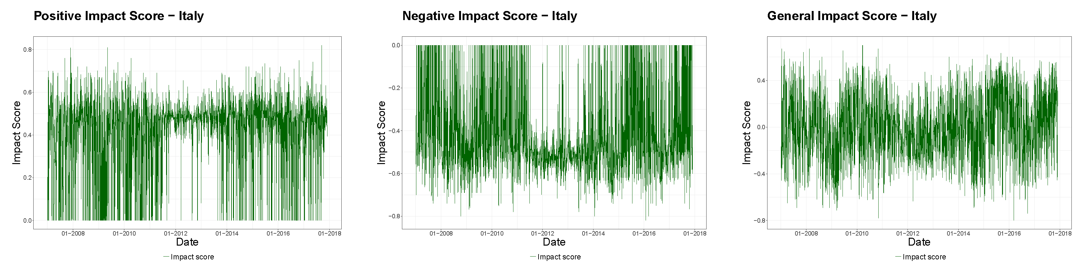
• a news-impact time series,

for the three categories

• all news,
• positive news,
• negative news.

We build the volume of news time series $V\left(t\right)$ with n denoting the number of news items and t with $t=Tr{D}_1,\dots ,Tr{D}_m$ denoting the current trading day, as

$$V\left(t\right)=\sum _{i=1}^n{1}_{\{TrD\left(N_i\right)=t\}}.$$

The mean news-sentiment time series takes into account the event sentiment score “ESS”, which is delivered with each news event, $-1\le ESS\le 1$. The mean overall sentiment scores are calculated for each trading day leading to a trading day mean news-sentiment time series. The mean news-sentiment value time series $MS\left(t\right)$ is calculated as

$$MS\left(t\right)=\frac{1}{V\left(t\right)}\sum _{j=1}^{V\left(t\right)}ESS\left(N_j\right)1_{\{TrD\left(N_i\right)=t\}}.$$

The news-impact time series takes into account the potential influence decay of a news story. The news items for each working day are weighted keeping in mind that the most recent news item before closing has the highest effect on the closing yield. The other news items, which come in before that, have a decaying importance. The news-impact time series $IS\left(t\right)$ with c denoting the closing time of the market is given as

$$IS\left(t\right)=\frac{1}{V\left(t\right)}\sum _{j=1}^{V\left(t\right)}ESS\left(N_j\right)e^{\lambda \left(c-time\left(N_j\right)\right)}{1}_{\{TrD\left(N_i\right)=t\}}.$$

The calculation of the news-impact time series was introduced by (Yu and Mitra 2016). The sentiment value $ESS$ is multiplied by a decreasing exponential weight leading to the news impact score $I,$ $I=ESS\ast e^{(-\lambda (c-time\left)\right)}.$ The closing time of the market c is the reference time, $c-time$ measures the difference between news time $time$ and market closing time and the decaying factor $\lambda$ is determined through $e^{(-\lambda (240\left)\right)}=1/2.$ We choose a time span of 640 min, after which news stories only have half of their impact left.

Time series of volume of the news items are examined as well. We count the number of relevant news items for the entity considered for a given trading day. Again, weekend news and news after market closing are shifted to the next trading day. We count all incoming news items (neutral, positive and negative) to create the volume of all news time series and distinguish between positive and negative news sentiment to create a volume of positive and negative news time series.

Therefore, we create nine different time series observed throughout the time interval where the bond is active. All news time series are utilized as regressors in a regression model as well as external variables in an ARIMAX model. Furthermore, their correlation with the yield spread is calculated for the whole time period and through a rolling window approach.

When analysing correlations between bond yields and news-sentiment time series, we have to consider potential spurious correlations we might observe due to business cycle effects or common market microstructures. When analysing the volume of news times series, we cannot detect long-term business cycle trends, rather short-term news event effects are captured quite clearly. The news-impact time series put the highest weights to most recent news, news older than 10 h does not have a high weight in the daily time series anymore. Therefore, we focus on capturing short-term macroeconomic news effects and analyse the correlation between bond spreads and these derived macroeconomic news-sentiment series.

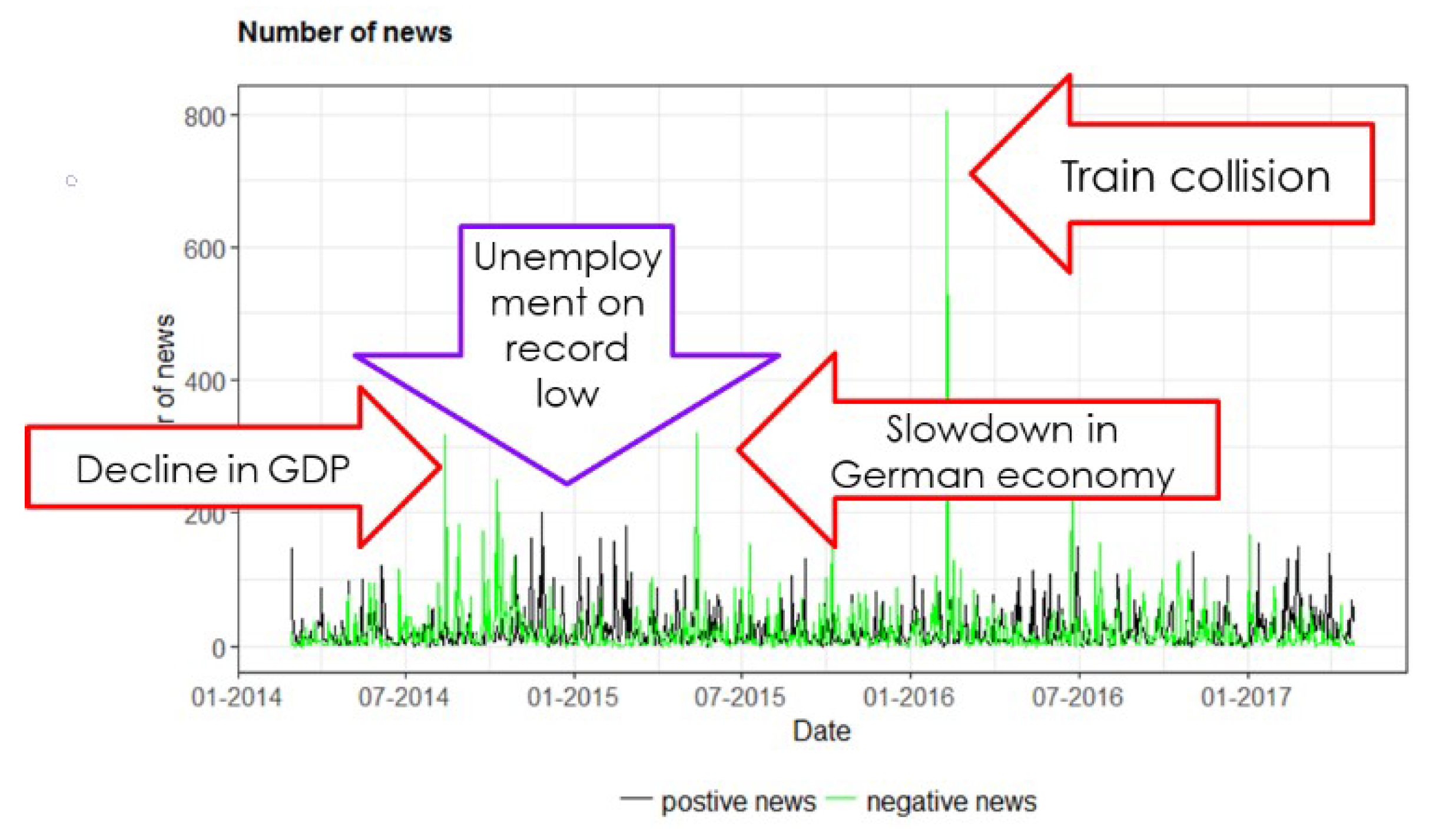
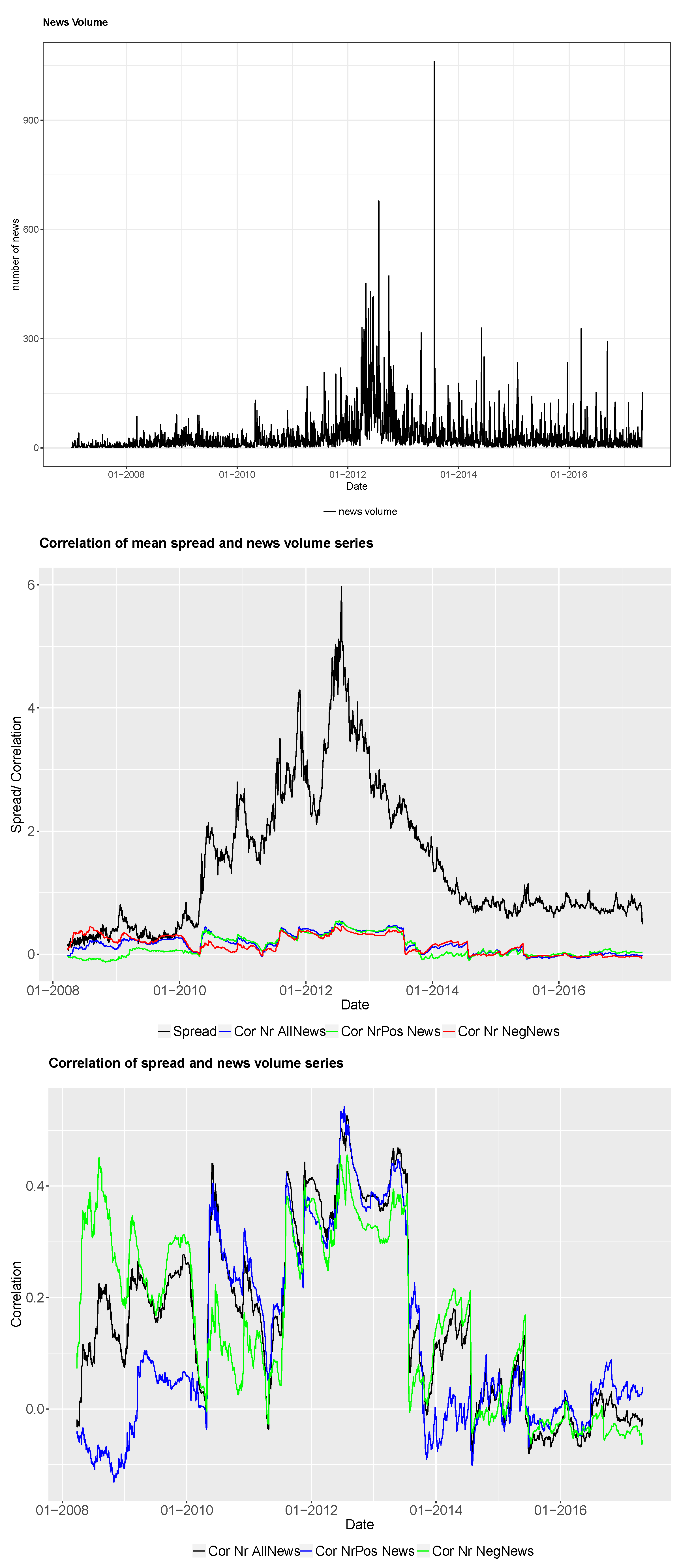
In Figure 1, a typical time series of news volume is depicted. Here, we show a volume series for Germany, where we distinguish between positive and negative news items. We can see spikes in the positive and negative volume series, which are analysed in more detail to understand the reason for this dynamic. Increases in positive and negative news are triggered through various events, which might not all be relevant for movements of bond spreads. Since we would like to analyse effects of macroeconomic news on bond spreads, we are less interested in news collected under the topic “social”; instead, we concentrate in the following on news from the broad topics “politics” and “economics”.

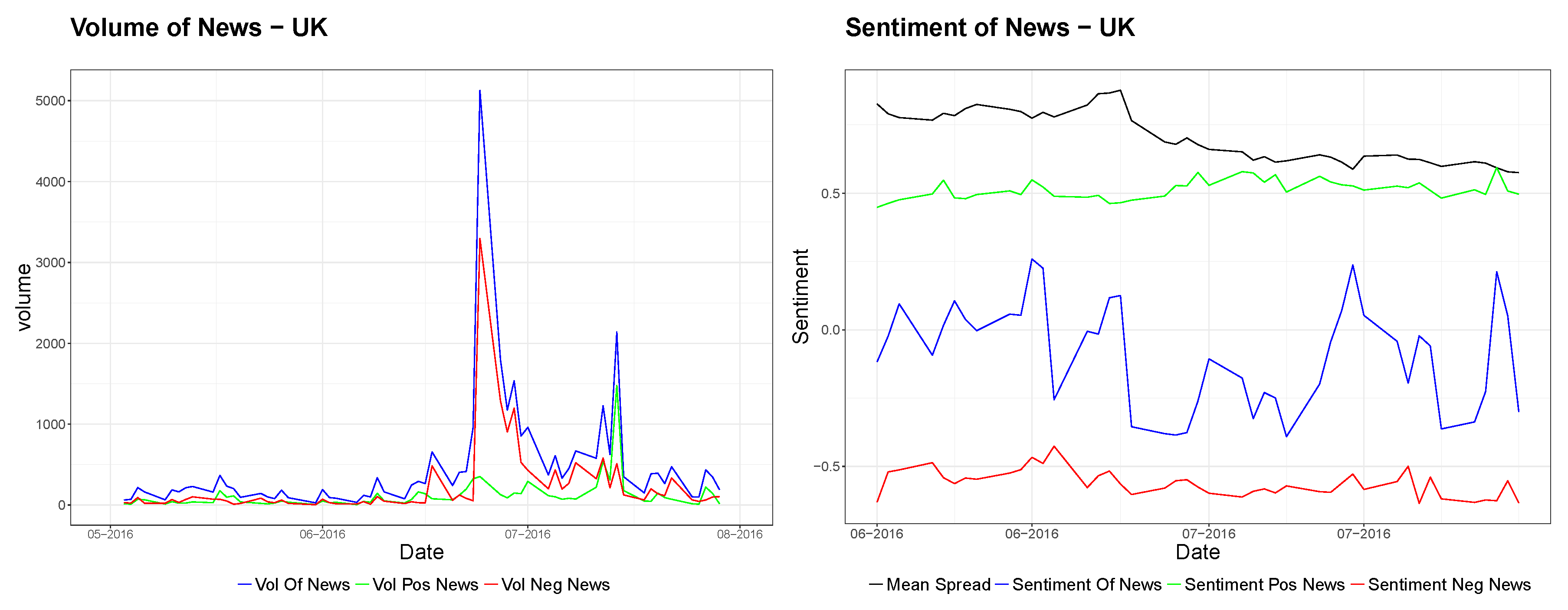
One important event that occurred in the covered time period has been the Brexit Referendum in the UK on 23 June 2016. In Figure 2, we depict the volume and sentiment of news of positive, negative and overall news events for the entity UK between May and July 2016. A clear spike in the volume of news can be detected on and shortly after 23 June. In addition, the overall sentiment shows a decline in this period; however, the sentiment series exhibits less movement during the referendum period. Here, the volume of macroeconomic news is a stronger signal for events than the daily sentiment series. This example highlights the different features of the daily sentiment series, counting the occurring news events which are relevant for an entity is often a good indication of market movements.

2.3. Correlation and ARIMAX Models

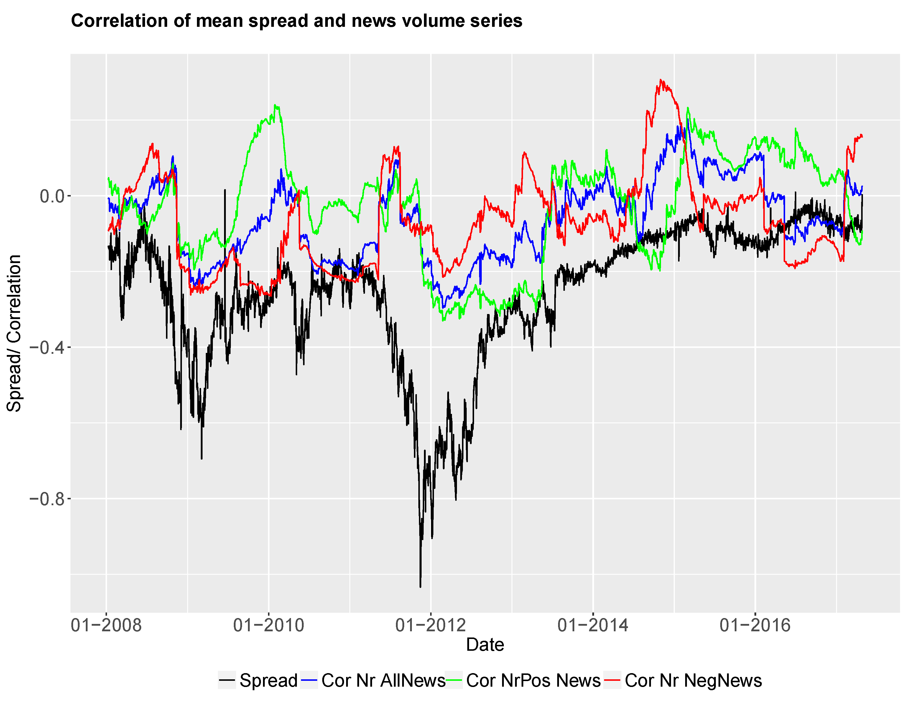
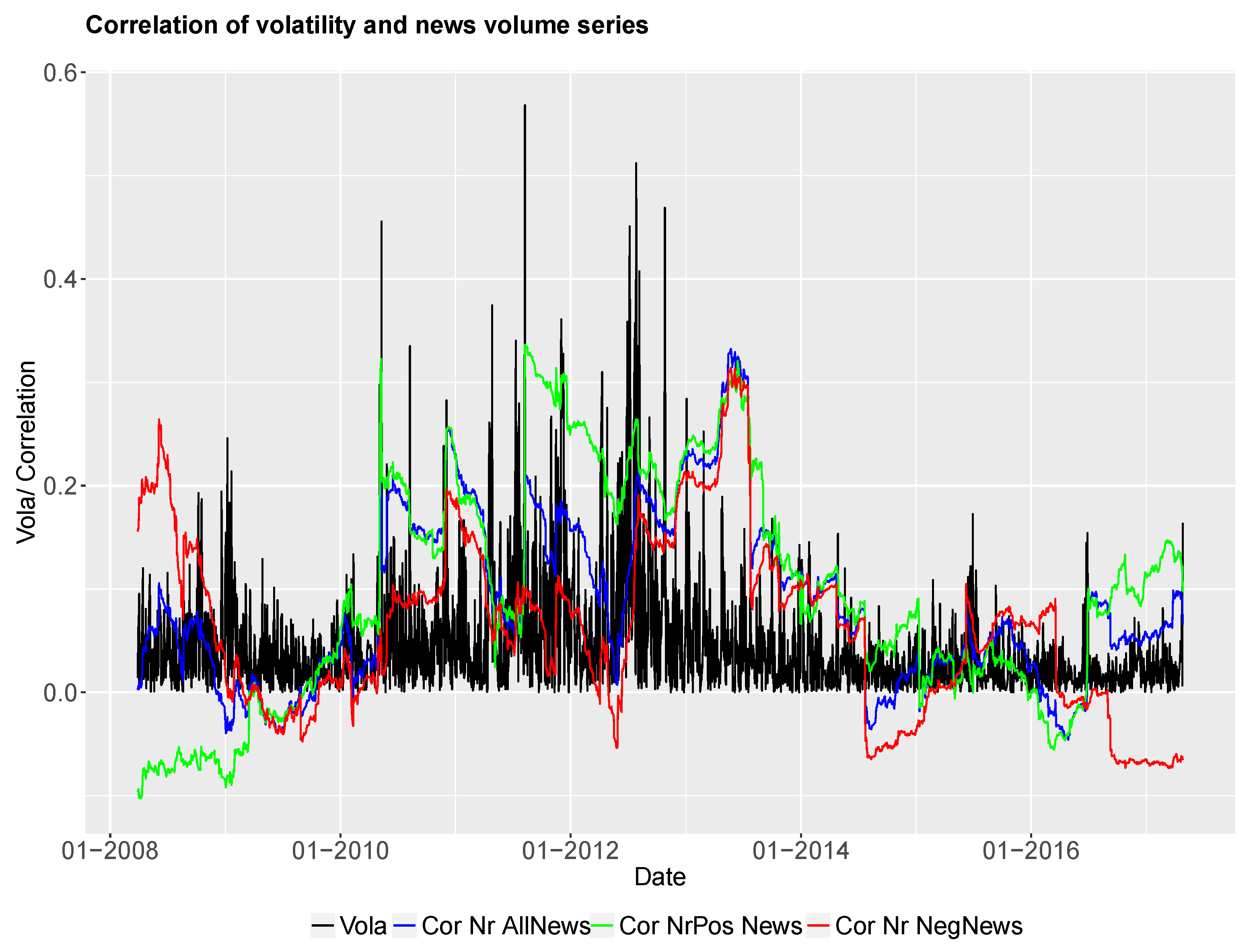
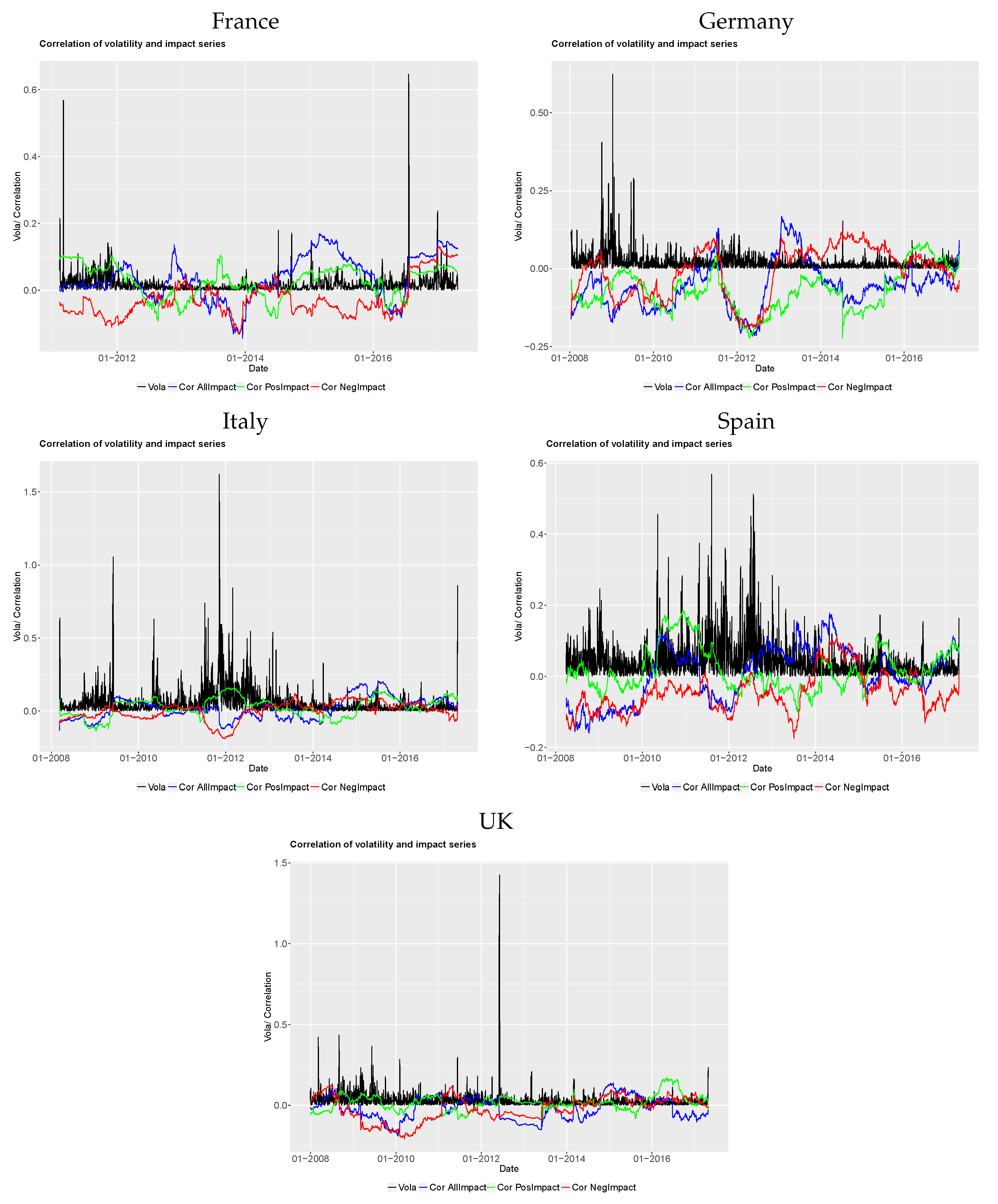
In order to establish whether a relation between the different news time series and the yield spread changes exists, we test for correlation between the daily spread change series and all nine news time series. We calculate Pearson’s correlation between the daily time series and test whether the correlation is significant. Furthermore, the correlation is estimated within a rolling window to see time-varying features of the correlation between time series. We would like to investigate stability and predictive accuracy over time.

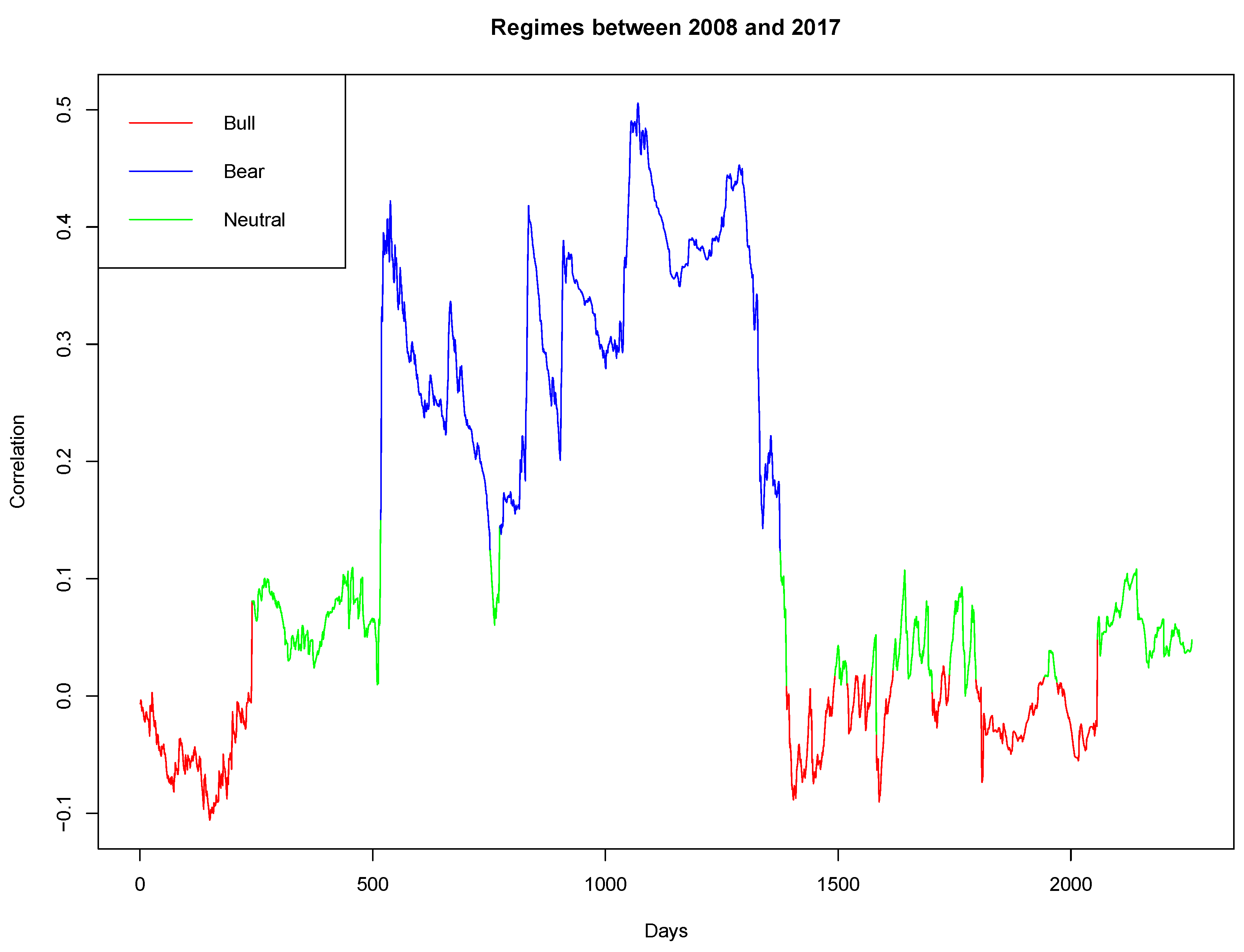
By calculating rolling correlations between daily news sentiment series and bond spread series, we establish the correlation through time. We would like to find out if the correlations are more or less stable over time or if we have large variations of correlation values. In particular, we are interested in investigating change points in the rolling correlation series. We assume that a significant change from positive to negative correlations indicates changes in the market environment. These changes can be captured in a regime-switching setting, where market states of the underlying bond spread can be filtered out by estimating the current state of the rolling correlation time series. In the literature, exogenous break points in sovereign bond spread series have been established in our considered time window between 2007 and 2017. The exogenous breaks often mark a division into pre- and post crisis periods (see, amongst others, (Afonso et al. 2015; Caggiano and Greco 2012)). Further methodologies to analyse a changing relationship between news time series and yield spreads over time include the Dynamic Conditional Correlation model by (Engle 2002) and the specific model formulation for leptokurtic data analysed in (Del Brio et al. 2011). In addition, a cointegration analysis can add further value, especially a threshold cointegration where adjustments occur when deviations reach a certain threshold (see, e.g., (Stigler 2010) for an overview and (Tsagkanos and Siriopoulos 2015) for a case study on asymmetric effects between markets and production in Northern and Southern Europe). These methodologies are promising alternatives and will be analysed in future work. We analyse our correlation findings further within a regime-switching setting, where hidden regime switches are estimated by filtering out information on the observed rolling correlation. News and their correlation to bond spreads are then analysed taking into account the current filtered market regime.

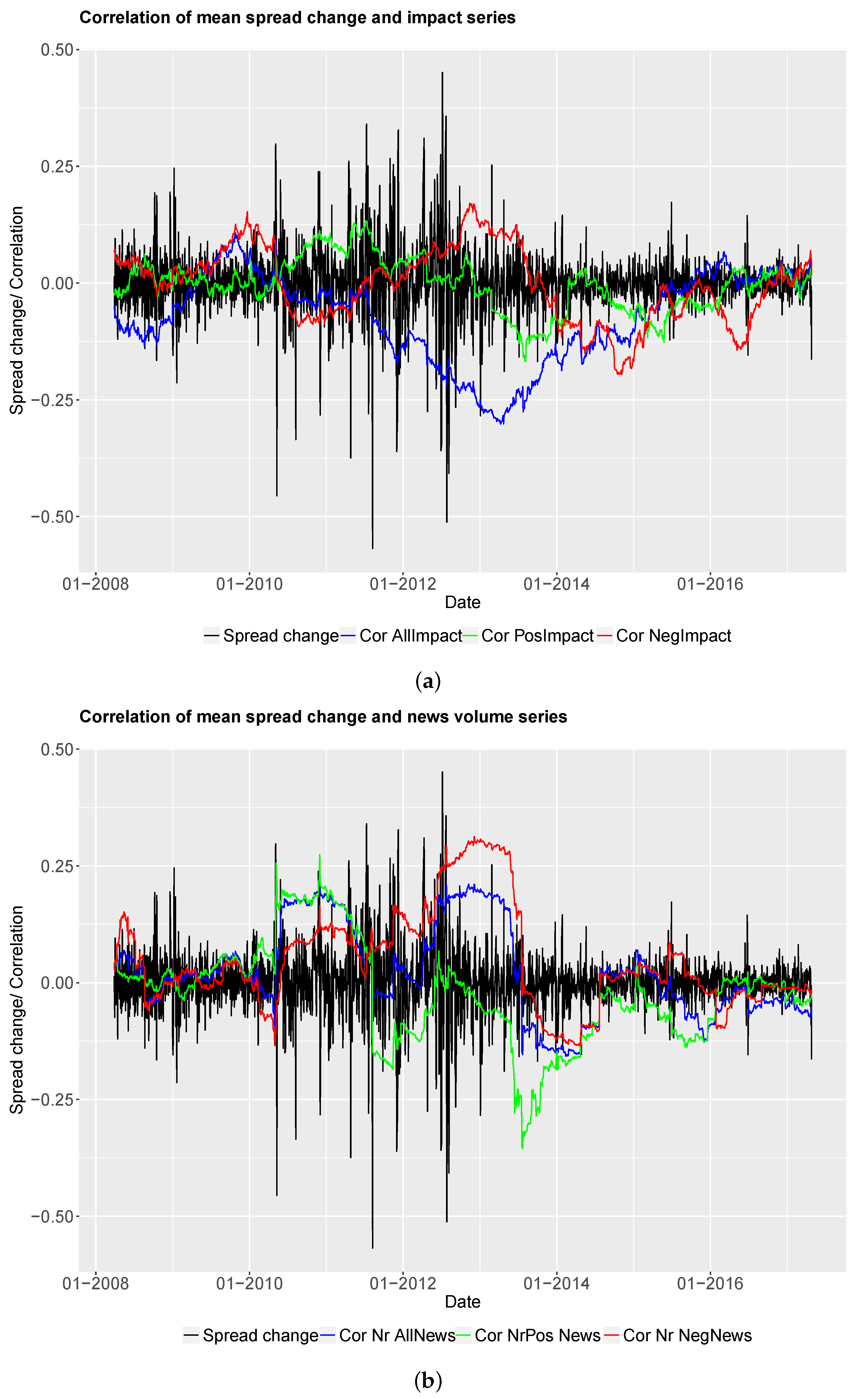
Secondly, a linear regression is performed to analyse the effects of news time series on the yield spread changes. All nine news time series are taken as regressors in a variety of combinations. We report here results for regression with three news series regressors, namely the Volume of All News, Positive Impact and Negative Impact.

Lastly, we apply an Integrated Autoregressive Moving Average (ARIMA) model (see (Tsay 2010) for more details) to analyse and forecast bond yields. We additionally add external explanatory variables to the model, therefore fitting an ARIMAX(p,i,q) model to yield spread changes. The ARIMAX(p,i,q) model is given through

$$d_t={\varphi }_0+\sum _{k=1}^p{\varphi }_k{d}_{t-k}+a_t+\sum _{k=1}^q{\theta }_k{a}_{t-k}+\sum _{l=1}^m{\psi }_l{x}_{lt}$$

(1)

where $d_t$ is the i-th differenced series of the time series $r_t,$ $\left\{a_t\right\}$ is a white noise series and $x_{lt}$ is the l-th external explanatory variable, $l=1,\dots ,m.$ The explanatory variable are uni- or multivariate. An ARIMAX model was also successfully applied by Apergis (2015) to analyse Credit Default Swaps (CDS) spreads and newswire sentiments. His study results in improved forecast errors when external news time series were allowed. We model the spread changes firstly with an ARIMA(p,i,q) model and compare the resulting in-sample and out-of-sample one-step ahead forecast errors to those which arise from ARIMAX(p,i,q) model with various external regressors. In the following sections, we run a considerable amount of models on our daily yield spread series, taking into account uni- as well as multivariate external explanatory variables. We can improve the forecast errors of analysed bonds when sentiment is taken into consideration. This points to the fact that news sentiment has a value for bond yield modelling and risk assessment. Monitoring macroeconomic news sentiment series in addition to the actual yield spread can lead to early warning signs for unexpected changes in yields or structural changes visible in the yield spreads.

3. Results and Discussion

We analyse sovereign bond spreads of five European countries and develop a sentiment-enhanced predictive modelling approach. We distinguish between short- and long-term bonds. In our categorization, short-term bonds have a maximum number of days to maturity of 1500.

3.1. Correlation and Market Regimes

First, we wish to investigate whether significant correlation can be found between spread time series from long-term bonds and our derived sentiment time series. The state of the markets, changes to it and therefore news that affect market behaviour have an effect on prices and spreads in the Fixed Income market. Up until now, less effort has been put into establishing the link between daily news sentiment and the dynamics of bond spreads.

We would like to analyse the correlation between the daily news sentiment series which were introduced above and bond spread changes. This leads us to restrict which of the news sentiment series shall be incorporated into the prediction of bond spreads. The daily news sentiment series have information on market movements and activities consolidated in a daily signal. We concentrate here on macroeconomic news to underline the effect that these news have on the sovereign risk of the issuer of the bond and therefore also on the bond spread. In equity markets, the question arises if the news or the market is quicker, meaning if news contains information which is not already reflected in the prices. This question is difficult to answer and there might be cases for both scenarios. However, Fixed Income markets in general are less likely to absorb macroeconomic information as fast as equity markets, since bond portfolios tend to be medium- to long-term investments and algorithmic trading decisions play a significant smaller role than in equity markets. We therefore use the daily macroeconomic news sentiment series as a source of information on current market affairs and market changes for the sovereign bonds. A correlation analysis gives us the insight whether a general connection between news signals and bond spread movements exists and, if so, how stable the correlation is and how news series can be utilised for daily predictions.

To conduct the correlation analysis, we create three spread time series, namely the spread series $S_t$, $t=1,\dots ,K,$ the first difference time series of this spread $D_t,$ $t=2,\dots ,K,$ and the volatility time series $V_t$ of $D_t,$ $t=2,\dots ,K.$ Our proxy volatility time series is calculated by taking the absolute value of $D_t,$ $t=1,\dots ,K.$ The duration of the bond in days is denoted by $K:$

$$\begin{array}{ccc}\hfill S_t& =& B_t-Y_t\hfill \\ \hfill D_t& =& S_t-S_{t-1}\hfill \\ \hfill V_t& =& |D_t|\hfill \end{array}$$

We denote the benchmark bond to calculate the spread by $B_t,$ the yield of the investigated bond is $Y_t.$ Time series $S_{jt},D_{jt}$ and $V_{jt}$ $j=1,\dots ,J,t=1,\dots ,K$ are calculated for all J bonds.

We calculate the rolling correlation between news and spread time series with a window size of 250 days. We analyse the significance of the correlation coefficient for each individual bond in our data set as well as for a mean spread time series $M_t,t=1,\dots ,N$ for each considered country. The time window covers the N days including all time intervals from all analysed long-term bonds. The mean spread is given by

$$M_t=\frac{1}{n_t}\sum _{j=1}^J{\mathbf{I}}_{\{S_{jt}\ne 0\}}{S}_{jt}$$

with $n_t$ denoting the number of available spreads at time $t.$ A mean spread is derived separately for each country, so that we can analyse thoroughly the country specifics.

3.2. Sovereign Bonds Spreads in Spain and Germany

Firstly, we analyse sovereign bonds issued by Spain. Over the last years, markets in Spain were in turmoil due to the European sovereign debt crisis. We expect to find changing correlations between the news sentiment series and Spanish bond spreads over the last years, especially between the years 2008 and 2015. These changing dynamics might have been influenced by European adjustment programs, e.g., the European Financial Stability Fund (EFSF) (see e.g., (Afonso et al. 2015)). The increased financial risk arisen from the sovereign debt crisis leads to a widening of sovereign bond spreads. The response from the European Union e.g., introducing EFSF had softening effects on correlation between fundamental risk factors and sovereign risk. Turbulent market times are also mirrored in more turbulent times in the news; therefore, we expect to find changing correlations over time.

We analyse the correlation between the Mean Spread series and the News Sentiment series and find significant correlation with “All Sentiment”,“All Impact” and “Volume of Neg News” and $D_t.$

Table 1. Percentage of significant correlations between spread and sentiment time series for long-term bonds issued by Spain.

Spain: News Time Series	${\mathit{S}}_{\mathit{t}}$	${\mathit{D}}_{\mathit{t}}$	${\mathit{V}}_{\mathit{t}}$
All Sentiment	66%	75%	47%
Volume All News	97%	31%	88%
All impact	50%	78%	28%
Positive Sentiment	78%	0%	56%
Volume Positive News	88%	37%	91%
Positive Impact	78%	0%	59%
Negative Sentiment	91%	3%	78%
Volume Negative News	97%	59%	84%
Negative Impact	91%	3%	78%

shows the percentages of bonds with significant correlations for each sentiment time series with $S_t,$ $D_t$ and $V_t$ for long-term bonds in Spain. The highest percentage of significant correlations arise with Volume of All and Volume of Negative News as well as with the time series on Negative Impact.

Furthermore, we depict the rolling correlation analysis on long-term bonds in Figure 3. The upper figure depicts the number of news items for the entity Spain between 2007 and 2017. It can clearly be seen that the news volume steadily increased between 2011 and 2014, a time where the sovereign debt crisis hit Spain, its companies and people. It is not surprising that the number of news increased in that period. Furthermore, the rolling correlation between the mean long-term spread and the news impact series is plotted in the second graph. An increase in correlation between news volume and long-term bond spreads can be detected between 2011 and 2014. It is noticeable that positive as well as negative news volume increased their correlation, both showing a positive correlation in times of crisis and large news volumes. This points to the fact that, overall, the volume is a well suited explanatory variable, highlighting the positive correlation between widening of sovereign spread and news volume. Analysing the news volume correlation time series in more detail, one can see that switching market regimes might lead to a switch in the direction of correlation. As can be seen in the third graph, between 2007 and 2009, the correlation between positive news volume and spread has been negative, indicating smaller spreads when more positive news were detected. However, this sign changed when the state of the market changed, leading to overall positive correlations between news volume and spread, regardless of the tone of the news. Therefore, in bear markets, the importance of the overall news volume is highlighted.

Furthermore, short-term bonds with a duration of less than 1500 days are analysed. In the following, all of the analysed bonds were issued by the Government of Spain between 2007 and 2017. We analyse 20 bonds, the spread, spread change and volatility of the spread series are calculated and their correlations with the sentiment series are estimated.

Table 2. Percentage of significant correlations between spread and sentiment time series for short-term bonds issued by Spain.

Spain: News Time Series	${\mathit{S}}_{\mathit{t}}$	${\mathit{D}}_{\mathit{t}}$	${\mathit{V}}_{\mathit{t}}$
All Sentiment	55%	30%	30%
Volume All News	70%	15%	50%
All impact	55%	25%	25%
Positive Sentiment	35%	0%	30%
Volume Positive News	60%	30%	60%
Positive Impact	40%	5%	25%
Negative Sentiment	60%	0%	30%
Volume Negative News	75%	30%	35%
Negative Impact	60%	5%	35%

shows the percentages of bonds with significant correlations for each sentiment time series with $S_t,$ $D_t$ and $V_t$ for 20 short-term bonds in Spain. We find that the volatility series are typically stronger correlated to the daily news-sentiment series than the spread difference. Sentiment series in this country for short-term bonds can be utilised to improve prediction of daily volatility. The sentiment series, especially the volume series of all news and the “All Sentiment” series, gives an additional insight for one-step ahead predictions of bond spread volatilities.

3.3. Market Regime Detection

To underpin the occurrence of changing regimes in the rolling correlation between sovereign bond spreads and the volume of news, we analyse the switching behaviour of the correlation time series. We assume an underlying Hidden Markov Model to find the best suitable state sequence. In a Hidden Markov Model, the market states are modelled through a Markov chain with a given number of states. The Markov chain is not observable but hidden in an observable market time series. Filtering out information of this hidden Markov chain through calculating conditional expected values leads to finding current state probabilities. Observable in the market are bond spreads and news items, their rolling correlation is calculated and taken as the observable time series. The actual state of the market is hidden in this correlation process, which becomes the observation process in our Hidden Markov model. We set the following definitions:

Definition 1

(Observation process). Let $\{y_t,t=1,\dots ,T\}$ denote a time series of T univariate observations taking values in a sampling space $\mathcal{Y},$ which may be either discrete or continuous. We consider $\{y_t,t=1,\dots ,T\}$ to be the realizations of the stochastic process ${\left\{Y_t\right\}}_{t=1}^T.$ We assume that the probability distribution depends on the realization of a hidden stochastic process $X_t.$ The stochastic process $Y_t$ is directly observable.

Definition 2

(Hidden process). Let $X_t$ be a discrete-time Markov chain with finite state space $I=\{1,\dots ,K\},$ which is irreducible and aperiodic starting from its ergodic distribution $\eta =({\eta }_1,\dots ,{\eta }_K).$ The transition probability matrix is denoted by $\Pi ,$ where each element ${\pi }_{jk}$ is the transition probability from state j to k. Thus, $P[X_0=k\mid \Pi ]={\eta }_k$ and $P[X_t=k\mid X_{t-1}=j]={\pi }_{jk}\forall j,k\in \{1,\dots ,K\}.$

The process $X_t$ is the hidden random process embedded in our observation process. The time series $\{y_1,\dots ,y_T\}$ is observed as realisation of a stochastic process $\{Y_1,\dots ,Y_T\},$ which is generated by a finite Markov mixture from the distribution family $Y_t\mid X_t\sim \mathcal{T}\left({\theta }_{X_t}\right).$ $X_t$ is an unobservable ergodic Markov chain with N states.

Consider the correlation series $Y_t$ which is modelled within a discrete-time HMM. We assume that $Y_t$ follows the dynamics

$$Y_t=\mu \left(X_t\right)+\sigma \left(X_t\right)z_t$$

(2)

where $\mu$ and $\sigma$ denote the drift and volatility of the time series, respectively, $z_t$ are independent and identically distributed (IID) normal random variables (IID) and $X_t$ denotes the Markov chain. Both $\mu$ and $\sigma$ are governed by the Markov chain $x_t.$

To analyse this, we fit a three-state Hidden Markov Model to the time series and adapt the Viterbi algorithm (see (Viterbi 1967)) for more details, for finding the optimal state sequence. Figure 4 depicts the estimated market state when analyzing the correlation between the mean bond spread of bonds issued by Spain and the volume of positive news. We can see here that the estimated market states are in line with the actual observed fact of widening credit spreads from 2011 to 2014. Before and after this period, the market in Spain is estimated to be neutral and in a bull state, which mirrors the real market situations in these larger time windows.

Additional information on Hidden Markov models and its estimation can be found in (Rabiner 1989) or (Elliott et al. 1995) amongst others. An in-depth analysis of changing market states and their effects on news sentiment influences is the topic of future work.

German bonds, which have been in a stable market within this time period, also exhibit changing rolling correlations over time. We depict the rolling correlation between the mean long-term spread issued by Germany and the volume of news items in Figure 5. It can be seen that, when the credit spread gets narrower and even becomes negative in 2011, the correlation between positive news volume and mean spread changes to negative, an increase in positive news is linked to a decrease in the bond spread. This is true since the Fixed Income market in Germany within this period is stable and not in a bear market.

3.4. Analysis of Mean Bond Spreads

In this section, we would like to focus our analysis on mean bond spreads from Spain, Germany, Italy, France and the UK. We consider here the mean spread at any given point in time over all available bond spreads in our database for each of the countries. When analysing the mean spread, we investigate in general the potential effect of including impact values and news volume for each entity as external variables. In particular, the correlation between bonds spread series and news time series shall be analysed, a linear regression is performed and a one-step ahead prediction (in- and out-of-sample) through an ARIMAX model is performed. This gives an understanding about the enhancement of predictions by involving external variables. The external news variables carry information on macro-economic changes and topics in the considered countries. Analysing the mean spread of a given bond portfolio leads to a general view on influence and correlations between macroeconomic news items and Fixed Income markets for a specific country.

First, we analyse the mean bond yield of 53 long- and short-term government bonds in Spain, which were active between 2007 and 2017. The mean bond yield and its first difference are calculated and the rolling correlation between this differenced series and the sentiment time series are estimated. The rolling correlation with a rolling window of 250 days is determined. The volatility proxy, which shows significant correlation with the Volume of News time series, leads to changing correlation patterns over time. We consider here the changing correlation between the volatility of the mean spread of all sovereign bonds from Spain in our dataset, which covers the time period between 2008 and 2017. Figure 6 depicts the rolling correlation between the volatility and the three Volume of News time series. The correlation with the Volume of All News changes from a negative to a positive correlation in times when the volatility increases. Again, when the markets start to be calmer, the rolling correlation value decreases. This pattern can be observed for the other analysed countries as well, leading to the fact that the Volume of All News is utilised as an informative time series for further predictions. In turbulent market times, the correlation between the Volume of All News time series and the volatility proxy fluctuates around $0.2;$ it decreases sharply when the markets enter a quieter period.

Figure 7 depicts the spread change $D_t$ of the mean of the Spain bond yield and the rolling correlation series. The window size is set to 250 days; correlation is calculated for six different time series, the impact values and the volume. Rolling correlation changes in particular when market circumstances change, again pointing to the fact that news have a different impact in different regimes and that shifts can be examined through the correlation with news volume.

We test for significant correlation and find that, considering only one time window, the correlation between the mean spread and the three time series for all news sentiment is significant at $\alpha =0.01.$ Correlations between the mean spread and the Sentiment and Impact series are negative, correlation with the time series of Volume of All News is positive. Furthermore, considering a linear regression, we find that the Volume of All News is a significant regressor.

Let us furthermore consider bond spreads from Germany, a rather stable economy within the European union in the considered time interval. The number of news covered for this entity between 2007 and 2017 is 360,864. When filtering for news with a relevance >60 and leaving out news from the topic “society”, the database has 167,359 news items within this time period which are considered for creating daily news time series. We find significant correlation $\rho$ between $V_t$, the volatility of the spread difference and the news time series All Sentiment $(\rho =-0.14)$, All Impact $(\rho =-0.14),$ Positive Sentiment $(\rho =-0.1),$ Volume of Positive News $(\rho =-0.04),$ Positive Impact $(\rho =-0.11),$ Negative Sentiment $(\rho =-0.06)$ and Negative Impact $(\rho =-0.06).$ All news time series are negatively correlated to the volatility of the bond spread difference, leading to the conclusion that lower sentiment and impact can be observed when higher volatility is present.

Linear Regression for Spread Volatility

Moving on from these correlation findings, we conduct a linear regression where the three time series “Volume of All News”, “Positive Impact” and “Negative Impact” are chosen as regressors. The results depicted in

Table 3. Regression analysis for volatility of German mean bond spread difference. Residual standard error: 0.02701 on 2582 degrees of freedom Multiple R-squared: 0.01342, Adjusted R-squared: 0.01227 F-statistic: 11.71 on 3 and 2582 DF, p-value: 1.288 × 10${}^{-7}$. Signif. codes are: 0 ‘***’ 0.001 ‘**’ 0.01 ‘*’ 0.05 ‘.’ 0.1 ‘ ’.

Coefficients:	Estimate	Std. Error	t Value	Pr (>|t|)
(Intercept)	2.488 × 10${}^{-2}$	2.804 × 10${}^{-3}$	8.871	<2 × 10${}^{-16}$	***
NrOfAllNews	−4.802 × 10${}^{-6}$	9.024 × 10${}^{-6}$	−0.532	0.594649
PosImpact	−2.385 × 10${}^{-2}$	4.842 × 10${}^{-3}$	−4.927	8.9 × 10${}^{-7}$	***
NegImpact	−1.265 × 10${}^{-2}$	3.583 × 10${}^{-3}$	−3.531	0.000421	***

show that the impact time series are significant regressors at a 0.1% level.

The regression results show that the positive and negative impact series are informative input variables for the volatility proxy. Both impact scores have negative coefficient estimates; therefore, positive news impact has a negative effect on the spread volatility, whereas negative impact (which takes values <0) has an increasing effect on volatilities. We receive similar regression results for the experiments on other countries’ volatility time series (see

Table 4. Regression analysis for volatility of the mean bond spread difference from Spain. Residual standard error: 0.05141 on 2505 degrees of freedom Multiple R-squared: 0.06588, Adjusted R-squared: 0.06476 F-statistic: 58.89 on 3 and 2505 DF, p-value: <2.2 × 10${}^{-16}$. Signif. codes are: 0 ‘***’ 0.001 ‘**’ 0.01 ‘*’ 0.05 ‘.’ 0.1 ‘ ’.

Coefficients:	Estimate	Std. Error	t Value	Pr (>|t|)
(Intercept)	2.476 × 10${}^{-2}$	3.372 × 10${}^{-3}$	7.343	2.81 × 10${}^{-13}$	***
NrOfAllNews	2.082 × 10${}^{-4}$	1.901 × 10${}^{-5}$	10.956	<2 × 10${}^{-16}$	***
PosImpact	2.710 × 10${}^{-3}$	5.657 × 10${}^{-3}$	0.479	0.632
NegImpact	−2.365 × 10${}^{-2}$	4.876 × 10${}^{-3}$	−4.850	1.31 × 10${}^{-6}$	***

,

Table 5. Regression analysis for volatility of mean bond spread difference from the UK. Residual standard error: 0.04189 on 2602 degrees of freedom Multiple R-squared: 0.005889, Adjusted R-squared: 0.004742 F-statistic: 5.138 on 3 and 2602 DF, p-value: 0.001526. Signif. codes are: 0 ‘***’ 0.001 ‘**’ 0.01 ‘*’ 0.05 ‘.’ 0.1 ‘ ’.

Coefficients:	Estimate	Std. Error	t Value	Pr (>|t|)
(Intercept)	3.145 × 10${}^{-2}$	9.323 × 10${}^{-3}$	3.373	0.000753	***
NrOfAllNews	−7.625 × 10${}^{-6}$	4.947 × 10${}^{-6}$	−1.541	0.123393
PosImpact	−3.579 × 10${}^{-2}$	1.457 × 10${}^{-2}$	−2.456	0.014109	*
NegImpact	−3.485 × 10${}^{-2}$	1.189 × 10${}^{-2}$	−2.931	0.003413	**

,

Table 6. Regression analysis for volatility of the mean bond spread difference from Italy. Residual standard error: 0.08624 on 2415 degrees of freedom Multiple R-squared: 0.1526, Adjusted R-squared: 0.1516 F-statistic: 145 on 3 and 2415 DF, p-value: <2.2 × 10${}^{-16}$. Signif. codes are: 0 ‘***’ 0.001 ‘**’ 0.01 ‘*’ 0.05 ‘.’ 0.1 ‘ ’.

Coefficients:	Estimate	Std. Error	t Value	Pr (>|t|)
(Intercept)	3.166 × 10${}^{-2}$	5.526 × 10${}^{-3}$	5.730	1.13 × 10${}^{-8}$	***
NrOfAllNews	4.022 × 10${}^{-4}$	1.997 × 10${}^{-5}$	20.145	<2 × 10${}^{-16}$	***
PosImpact	9.936 × 10${}^{-3}$	9.451 × 10${}^{-3}$	1.051	0.293
NegImpact	−1.279 × 10${}^{-2}$	8.609 × 10${}^{-3}$	−1.486	0.137

and

Table 7. Regression analysis for volatility of the mean bond spread difference for France. Residual standard error: 0.02362 on 1793 degrees of freedom Multiple R-squared: 0.00222, Adjusted R-squared: 0.0005506 F-statistic: 1.33 on 3 and 1793 DF, p-value: 0.263. Signif. codes are: 0 ‘***’ 0.001 ‘**’ 0.01 ‘*’ 0.05 ‘.’ 0.1 ‘ ’.

Coefficients:	Estimate	Std. Error	t Value	Pr (>|t|)
(Intercept)	1.755 × 10${}^{-2}$	2.087 × 10${}^{-3}$	8.411	<2 × 10${}^{-16}$	***
NrOfAllNews	−4.636× 10${}^{-6}$	9.721 × 10${}^{-6}$	−0.477	0.6335
PosImpact	3.435 × 10${}^{-3}$	3.681 × 10${}^{-3}$	0.933	0.3508
NegImpact	4.680 × 10${}^{-3}$	2.783 × 10${}^{-3}$	1.681	0.0929	.

). For the spread volatility from Italy, we receive significant estimates for the volume of all news regressors, for Spain, the UK and France, the negative news impact is a significant regressor. We conclude therefore that derived regressors from macro news sentiment have an effect on these sovereign bond spread volatilities.

Furthermore, we analyse the correlation between the mean bond spread volatilities and the impact scores. We exemplarily depict positive, negative and general impact scores from Italy in Figure 8. We see that the mean level for the positive impact score time series is roughly at 0.4; the mean level of the negative impact score time series is around $-0.4$. An increase in negative scores therefore means a value closer to zero. In Figure 9, we then depict the rolling correlation between the volatility of the mean bond spread and the impact scores for the five countries.

Figure 9 shows how the correlation changes over time. As was pointed out in the previous section, correlation patterns change and have varying signs in varying market states. By comparing the rolling correlation dynamics in the five European countries, we see that the correlation between the impact values of news and the volatility mainly fluctuates in a range between $-0.2$ and 0.2. On average, there is a negative correlation between the negative impact scores and the volatility of the news. When the negative impact score rises, the volatility decreases.

4. Prediction of Sovereign Bond Spreads through News Sentiment

We now turn our focus on the enhancement of predicting future bond spreads through macroeconomic news sentiment. Our previous results on correlation in both static and rolling windows as well as on linear regression with daily news sentiment time series lead us to utilise news sentiment time series as an external variable in an Integrated Autoregressive Moving Average Model with explanatory variables (ARIMAX).

After testing for best suited order parameters, we perform fitting and forecasting an ARIMAX(2,0,2) model on 51 sovereign bonds issued by Germany. We model the spread difference series $D_t,$ choose different external variables and compare five model set-ups:

ARIMAX Model	External Variables
ARIMAX 1	No external variable
ARIMAX 2	Positive Impact; Negative Impact
ARIMAX 3	Volume of All News; All Impact
ARIMAX 4	Volume of Positive News
ARIMAX 5	Volume of All News

An error analysis shows that adding external variables decreases the forecast error in both the in-sample and out-of-sample period. The length of the out-of-sample period is chosen as 15% of the length of the time series.

Table 8. Error distribution of ARIMAX models for in-sample and out-of-sample window of analysis of sovereign bonds issued by Germany. The highlighted data show the lowest Median RMSE over all models.

	ARIMAX 1	ARIMAX 2	ARIMAX 3	ARIMAX 4	ARIMAX 5
In-Sample
Min.	0.01424	0.01400	0.01418	0.01421	0.01424
1st Quartile	0.02337	0.02328	0.02326	0.02334	0.02327
Median	0.02930	0.02895	0.02924	0.02926	0.02925
Mean	0.04532	0.04492	0.04478	0.04513	0.04496
3rd Quartile	0.04043	0.04015	0.04036	0.04042	0.04037
Max.	0.41261	0.41258	0.41236	0.41233	0.41244
Out-of-Sample
Min.	0.01430	0.01431	0.01430	0.01432	0.01430
1st Quartile	0.02147	0.02251	0.02233	0.02256	0.02152
Median	0.03570	0.03537	0.03513	0.03547	0.03513
Mean	0.05260	0.05307	0.05300	0.05291	0.05280
3rd Quartile	0.06758	0.06843	0.06808	0.06795	0.06776
Max.	0.33667	0.32860	0.33296	0.33527	0.33662

shows the empirical error distribution of each model. The lowest median Root Mean Squared Error (RMSE) is reached by ARIMAX 2 (in-sample) and ARIMAX 3 (out-of-sample).

We further analyse that when modelling daily spread differences the lowest RMSE in the in-sample period is gained through Model ARIMAX 2 (in 55% of cases), followed by Model ARIMAX 3 (in 33%). For the out-of-sample period, we find that the lowest RMSE is obtained through Model ARIMAX 2 (in 31%) followed by Model ARIMAX 1 (in 23%). A similar pattern arises when the volatility proxy is predicted.

For the UK, we analyse 100 sovereign bonds, 28 long-term and 72 short-term bonds. We predict the spread changes as well as the volatility with the same model set-up as explained above and find that the lowest RMSE in the in- and out-of-sample set-up is reached by Model ARIMAX 2 (60% and 32% of bonds) and Model ARIMAX 3 (30% and 26% of bonds).

We conclude that, for both countries, the predictions of spread changes from single bonds are best enhanced by Positive and Negative Impact series as external variables as well as Volume and Impact of All News. The forecast error of predicting volatility is also improved when impact series and volume series of all news are taken into account. The risk assessment can therefore be enhanced through adding these macroeconomic news series.

Countries’ Mean Bond Spreads

We now perform the ARIMAX analysis on the mean bond spread for each European country we consider. We calculate for each point in time the mean spread value of the bonds available in the dataset of each country. This mean value is taken as a reference bond spread for the country at a given point in time, which reflects the typical movements and therefore risks of the issued sovereign bonds. We hereby consider both long-and short-term bonds.

Furthermore, we compare the performance of the prediction through ARIMAX models in the different European countries. We analyse the model performance by setting the first 85% of the length of each time series as in-sample and the last interval as the out-of-sample period. When modelling the first difference of the mean bond spread, we set the explanatory variable in ARIMAX 4 to the Volume of Negative News and in ARIMAX 5 to All Impact, since these variables have a stronger impact on the prediction than Volume of Positive News and Volume of All News, which are chosen when the volatility proxy is modelled.

First, we calculate the Akaike Information Criterion (AIC) for each model set-up to see whether including external variables result in an improvement compared to the standard ARIMA model when modelling the first difference and the volatility proxy of each country’s mean spread. The AIC is calculated for each country and model and the results are presented in

Table 9. AIC for all models and countries for modelling first difference of mean spread.

Country	ARIMAX 1	ARIMAX 2	ARIMAX 3	ARIMAX 4	ARIMAX 5
Spain	−4955.11	−4951.16	−4960.94	−4961.23	−4961.48
Germany	−7908.22	−7905.09	−7904.37	−7906.39	−7906.37
UK	−6141.76	−6143.39	−6142.24	−6139.86	−6143.06
Italy	−2828.18	−2824.33	−2856.49	−2869.29	−2841.23
France	−6151.18	−6150.12	−6148.75	−6149.49	−6150.58

and

Table 10. AIC for all model and countries for modelling volatility proxy of mean spread.

Country	ARIMAX 1	ARIMAX 2	ARIMAX 3	ARIMAX 4	ARIMAX 5
Spain	−6383.28	−6379.91	−6381.87	−6392.53	−6383.87
Germany	−8709.1	−8720.27	−8718.92	−8707.35	−8707.16
UK	−7161.99	−7159.02	−7152.87	−7161.13	−7145.24
Italy	−4029.1	−4025.82	−4226.42	−4089	−4224.94
France	−6768.78	−6766.79	−6768.88	−6767.23	−6770.87

; the best AIC value per country is highlighted. We see that, in most cases, adding external variables improves the AIC value of the model. However, the best external variable differs depending on the country.

The error analysis of the mean bond spread results in RMSE values can be seen in

Table 11. RMSE for in-sample period of ARIMAX models for mean country spread difference.

Country	ARIMAX 1	ARIMAX 2	ARIMAX 3	ARIMAX 4	ARIMAX 5
Spain	0.070017	0.070016	0.069845	0.069875	0.069871
Germany	0.035505	0.035497	0.035504	0.035503	0.035504
UK	0.055108	0.055034	0.055049	0.055107	0.055065
Italy	0.115992	0.115988	0.115026	0.114704	0.115541
France	0.028150	0.028121	0.028135	0.028147	0.028136

and

Table 12. RMSE for out-of-sample period of ARIMAX models for mean country spread difference.

Country	ARIMAX 1	ARIMAX 2	ARIMAX 3	ARIMAX 4	ARIMAX 5
Spain	0.033116	0.033145	0.033686	0.033288	0.033648
Germany	0.015860	0.015853	0.015883	0.015878	0.015882
UK	0.024518	0.024727	0.025383	0.024847	0.024373
Italy	0.035764	0.035781	0.040910	0.044636	0.037804
France	0.030514	0.030528	0.030511	0.030509	0.030512

for the analysed mean spread change for five countries for in- and out-of sample periods. We consider roughly 50 bonds in Spain, Germany and Italy between 2007 and 2017; for France and the UK, we analyse around 100 sovereign bonds. The results show that including sentiment series as an external variable improves the forecast both in the in-sample and out-of-sample period. Models ARIMAX 2 and ARIMAX 3 are the best performing model set-ups. Choosing the news impact time series as well as the volume of all news as external variables improves the one-step ahead prediction of the spread change. For each country, the prediction of the mean spread change can be improved when news time series are utilised.

Our analysis is done furthermore on the volatility proxy; the absolute value of the mean bond spread changes. Here, we find a similar result. Again, using sentiment news time series as an input variable decreases the RMSE of the one-step ahead forecast.

Table 13. RMSE for in-sample period of ARIMAX models for mean country volatility.

Country	ARIMAX 1	ARIMAX 2	ARIMAX 3	ARIMAX 4	ARIMAX 5
France	0.035559	0.035486	0.035510	0.035481	0.035514
Germany	0.028480	0.028455	0.028443	0.028478	0.028480
Italy	0.084966	0.084950	0.080648	0.083615	0.080722
Spain	0.049003	0.048996	0.048972	0.048867	0.048972
UK	0.054074	0.053979	0.053868	0.054074	0.054054

and

Table 14. RMSE for out-of-sample period of ARIMAX models for mean country volatility.

Country	ARIMAX 1	ARIMAX 2	ARIMAX 3	ARIMAX 4	ARIMAX 5
France	0.047645	0.048033	0.047683	0.047741	0.047616
Germany	0.012011	0.012087	0.012076	0.012003	0.012009
Italy	0.027662	0.027744	0.047507	0.028939	0.047335
Spain	0.021855	0.021876	0.021889	0.022415	0.021893
UK	0.018621	0.019222	0.020254	0.018591	0.019527

depict the RMSE for the five countries in in- and out-of-sample periods.. We therefore conclude that news time series with our derived daily news signals are a valuable input variable and contain information to forecast spread changes and its volatility. The volatility forecast as a measure for risk is enhanced when daily news sentiment of each country is considered. The risk assessment is more accurate when macroeconomic news is taken into account.

We furthermore test whether the coefficients are significant in our model settings for the volatility and whether significant explanatory variables differ for each country. In

Table 15. z-test of coefficients for ARIMAX models in France for first difference of mean country spread. Signif. codes are: 0 ‘***’ 0.001 ‘**’ 0.01 ‘*’ 0.05 ‘.’ 0.1 ‘ ’.

France
ARIMAX 1
	Estimate	Std. Error	z value	Pr (>|z|)
ma1	0.1570987	0.0269996	5.8186	5.936 × 10${}^{-9}$	***
ma2	0.1419447	0.0243265	5.8350	5.380 × 10${}^{-9}$	***
intercept	0.0162441	0.0007797	20.8338	<2.2 × 10${}^{-16}$	***
ARIMAX 2
	Estimate	Std. Error	z value	Pr (>|z|)
ma1	0.1589004	0.0270083	5.8834	4.019 × 10${}^{-9}$	***
ma2	0.1417316	0.0242918	5.8345	5.394 × 10${}^{-9}$	***
intercept	0.0158352	0.0023098	6.8556	7.103 × 10${}^{-12}$	***
Pos Impact	0.0040005	0.0038430	1.0410	0.2979
Neg Impact	0.0031073	0.0030199	1.0290	0.3035
ARIMAX 3
	Estimate	Std. Error	z value	Pr (>|z|)
ma1	1.5698 × 10${}^{-1}$	2.7021 × 10${}^{-2}$	5.8097	6.260 × 10${}^{-9}$	***
ma2	1.4238 × 10${}^{-1}$	2.4296 × 10${}^{-2}$	5.8602	4.624 × 10${}^{-9}$	***
intercept	1.6286 × 10${}^{-2}$	8.6834 × 10${}^{-4}$	18.7556	<2.2 × 10${}^{-16}$	***
All Impact	4.0236 × 10${}^{-3}$	2.0067 × 10${}^{-3}$	2.0051	0.04495	*
Vol of All News	−1.2558 × 10${}^{-6}$	2.8315 × 10${}^{-5}$	−0.0444	0.96463
ARIMAX 4
	Estimate	Std. Error	z value	Pr (>|z|)
ma1	1.5643 × 10${}^{-1}$	2.7021 × 10${}^{-2}$	5.7892	7.074 × 10${}^{-9}$	***
ma2	1.4215 × 10${}^{-1}$	2.4340 × 10${}^{-2}$	5.8402	5.214 × 10${}^{-9}$	***
intercept	1.6379 × 10${}^{-2}$	8.0711 × 10${}^{-4}$	20.2929	<2.2 × 10${}^{-16}$	***
Vol Neg News	−9.4690 × 10${}^{-6}$	2.9785 × 10${}^{-5}$	−0.3179	0.7506
ARIMAX 5
	Estimate	Std. Error	z value	Pr (>|z|)
ma1	0.15708778	0.02698884	5.8205	5.868 × 10${}^{-9}$	***
ma2	0.14238103	0.02429455	5.8606	4.612 × 10${}^{-9}$	***
intercept	0.01624505	0.00077884	20.8579	<2.2 × 10${}^{-16}$	***
All Impact	0.00404174	0.00199765	2.0232	0.04305	*

,

Table 16. z-test of coefficients for ARIMAX models in Germany for first difference of mean country spread. Signif. codes are: 0 ‘***’ 0.001 ‘**’ 0.01 ‘*’ 0.05 ‘.’ 0.1 ‘ ’.

Germany
ARIMAX 1
	Estimate	Std. Error	z value	Pr (>|z|)
ar1	−3.6493 × 10${}^{-2}$	9.4180 × 10${}^{-2}$	−0.3875	0.6984003
ar2	−1.0804 × 10${}^{-1}$	3.8524 × 10${}^{-2}$	−2.8045	0.0050388	**
ma1	−3.1595 × 10${}^{-1}$	9.3749 × 10${}^{-2}$	−3.3702	0.0007512	***
intercept	−4.5338 × 10${}^{-5}$	4.4661 × 10${}^{-4}$	−0.1015	0.9191406
ARIMAX 2
	Estimate	Std. Error	z value	Pr (>|z|)
ar1	−0.0396688	0.0944553	−0.4200	0.6745037
ar2	−0.1085231	0.0385408	−2.8158	0.0048656	**
ma1	−0.3132387	0.0941024	−3.3287	0.0008725	***
	Estimate	Std. Error	z value	Pr (>|z|)
intercept	−0.0028227	0.0033941	−0.8317	0.4055958
Pos Impact	0.0042479	0.0057224	0.7423	0.4578843
Neg Impact	−0.0014718	0.0042487	−0.3464	0.7290285
ARIMAX 3
	Estimate	Std. Error	z value	Pr (>|z|)
ar1	−4.0451 × 10${}^{-2}$	9.3563 × 10${}^{-2}$	−0.4323	0.6654925
ar2	−1.0967 × 10${}^{-1}$	3.8287 × 10${}^{-2}$	−2.8644	0.0041780	**
ma1	−3.1253 × 10${}^{-1}$	9.3140 × 10${}^{-2}$	−3.3555	0.0007923	***
intercept	2.9294 × 10${}^{-4}$	8.2730 × 10${}^{-4}$	0.3541	0.7232734
All Impact	−5.6466 × 10${}^{-4}$	2.4362 × 10${}^{-3}$	−0.2318	0.8167073
Vol All News	−6.1672 × 10${}^{-6}$	3.2677 × 10${}^{-5}$	−0.1887	0.8503033
ARIMAX 4
	Estimate	Std. Error	z value	Pr (>|z|)
ar1	−3.8931 × 10${}^{-2}$	9.3731 × 10${}^{-2}$	−0.4154	0.6778841
ar2	−1.0907 × 10${}^{-1}$	3.8331 × 10${}^{-2}$	−2.8455	0.0044348	**
ma1	−3.1403 × 10${}^{-1}$	9.3339 × 10${}^{-2}$	−3.3644	0.0007672	***
intercept	1.0767 × 10${}^{-4}$	5.8730 × 10${}^{-4}$	0.1833	0.8545389
Vol Neg News	−7.9893 × 10${}^{-6}$	3.1632 × 10${}^{-5}$	−0.2526	0.8006021
ARIMAX 5
	Estimate	Std. Error	z value	Pr (>|z|)
ar1	−4.0580 × 10${}^{-2}$	9.3979 × 10${}^{-2}$	−0.4318	0.6658911
ar2	−1.0948 × 10${}^{-1}$	3.8339 × 10${}^{-2}$	−2.8556	0.0042957	**
ma1	−3.1199 × 10${}^{-1}$	9.3603 × 10${}^{-2}$	−3.3332	0.0008587	***
intercept	−2.7963 × 10${}^{-5}$	4.5456 × 10${}^{-4}$	−0.0615	0.9509479
All Impact	−4.9344 × 10${}^{-4}$	2.4336 × 10${}^{-3}$	−0.2028	0.8393225

,

Table 17. z-test of coefficients for ARIMAX models in Italy for first difference of mean country spread. Signif. codes are: 0 ‘***’ 0.001 ‘**’ 0.01 ‘*’ 0.05 ‘.’ 0.1 ‘ ’.

Italy
ARIMAX 1
	Estimate	Std. Error	z value	Pr (>|z|)
ar1	0.46133768	0.12335966	3.7398	0.0001842	***
ar2	0.03544736	0.03389688	1.0457	0.2956806
ma1	−0.62378812	0.12090617	−5.1593	2.479 × 10${}^{-7}$	***
intercept	0.00018773	0.00197467	0.0951	0.9242594
ARIMAX 2
	Estimate	Std. Error	z value	Pr (>|z|)
ar1	0.46277654	0.12319101	3.7566	0.0001723	***
ar2	0.03559929	0.03388776	1.0505	0.2934856
ma1	−0.62498542	0.12072233	−5.1770	2.254 × 10${}^{-7}$	***
intercept	−0.00176552	0.00760684	−0.2321	0.8164635
Pos Impact	−0.00014615	0.01336217	−0.0109	0.9912732
Neg Impact	−0.00470141	0.01234966	−0.3807	0.7034323
ARIMAX 3
	Estimate	Std. Error	z value	Pr (>|z|)
ar1	5.0517 × 10${}^{-1}$	1.0053 × 10${}^{-1}$	5.0250	5.034 × 10${}^{-7}$	***
ar2	4.0360 × 10${}^{-2}$	3.1541 × 10${}^{-2}$	1.2796	0.2006900
ma1	−6.7218 × 10${}^{-1}$	9.7445 × 10${}^{-2}$	−6.8980	5.273 × 10${}^{-12}$	***
intercept	−4.1680 × 10${}^{-3}$	2.0572 × 10${}^{-3}$	−2.0261	0.0427560	*
All Impact	−3.0439 × 10${}^{-2}$	9.1134 × 10${}^{-3}$	−3.3400	0.0008377	***
Vol All News	1.0598 × 10${}^{-4}$	3.4367 × 10${}^{-5}$	3.0837	0.0020445	**
ARIMAX 4
	Estimate	Std. Error	z value	Pr (>|z|)
ar1	5.3473 × 10${}^{-1}$	8.6187 × 10${}^{-2}$	6.2043	5.494e-10	***
ar2	4.3724 × 10${}^{-2}$	3.0037 × 10${}^{-2}$	1.4557	0.14549
ma1	−7.0321 × 10${}^{-1}$	8.2556 × 10${}^{-2}$	−8.5180	<2.2 × 10${}^{-16}$	***
intercept	−3.6287 × 10${}^{-3}$	1.9272 × 10${}^{-3}$	−1.8829	0.05971	.
Vol Neg News	2.3325 × 10${}^{-4}$	4.2094 × 10${}^{-5}$	5.5412	3.003e-08	***
ARIMAX 5
	Estimate	Std. Error	z value	Pr (>|z|)
ar1	0.4378483	0.1385411	3.1604	0.0015754	**
ar2	0.0345230	0.0358910	0.9619	0.3361083
ma1	−0.6024669	0.1363825	−4.4175	9.986 × 10${}^{-6}$	***
intercept	−0.0010503	0.0020071	−0.5233	0.6007710
All Impact	−0.0353804	0.0091396	−3.8711	0.0001083	***

,

Table 18. z-test of coefficients for ARIMAX models in Spain for first difference of mean country spread. Signif. codes are: 0 ‘***’ 0.001 ‘**’ 0.01 ‘*’ 0.05 ‘.’ 0.1 ‘ ’.

Spain
ARIMAX 1
	Estimate	Std. Error	z value	Pr (>|z|)
ar1	0.95264611	0.07344346	12.9711	<2.2 × 10${}^{-16}$	***
ar2	−0.31051240	0.02587822	−11.9990	<2.2 × 10${}^{-16}$	***
ma1	−0.60989499	0.07476256	−8.1578	3.413 × 10${}^{-16}$	***
intercept	0.00025918	0.00170650	0.1519	0.8793
ARIMAX 2
	Estimate	Std. Error	z value	Pr (>|z|)
ar1	0.95221352	0.07374859	12.9116	<2.2 × 10${}^{-16}$	***
ar2	−0.31029570	0.02594255	−11.9609	<2.2 × 10${}^{-16}$	***
ma1	−0.60927154	0.07510366	−8.1124	4.963 × 10${}^{-16}$	***
intercept	0.00087810	0.00519333	0.1691	0.8657
Pos Impact	0.00032176	0.00824912	0.0390	0.9689
Neg Impact	0.00162662	0.00748399	0.2173	0.8279
ARIMAX 3
	Estimate	Std. Error	z value	Pr (>|z|)
ar1	9.5654 × 10${}^{-1}$	7.2633 × 10${}^{-2}$	13.1694	<2.2 × 10${}^{-16}$	***
ar2	−3.0813 × 10${}^{-1}$	2.5501 × 10${}^{-2}$	−12.0828	<2.2 × 10${}^{-16}$	***
ma1	−6.2122 × 10${}^{-1}$	7.3874 × 10${}^{-2}$	−8.4091	<2.2 × 10${}^{-16}$	***
intercept	−1.5055 × 10${}^{-3}$	1.9408 × 10${}^{-3}$	−0.7757	0.437934
All Impact	−1.4101 × 10${}^{-2}$	5.0149 × 10${}^{-3}$	−2.8118	0.004926	**
Vol All News	3.3985 × 10${}^{-5}$	3.5864 × 10${}^{-5}$	0.9476	0.343331
ARIMAX 4
	Estimate	Std. Error	z value	Pr (>|z|)
ar1	9.5207 × 10${}^{-1}$	7.4309 × 10${}^{-2}$	12.8123	<2.2 × 10${}^{-16}$	***
ar2	−3.0659 × 10${}^{-1}$	2.5850 × 10${}^{-2}$	−11.8600	<2.2 × 10${}^{-16}$	***
ma1	−6.1608 × 10${}^{-1}$	7.5588 × 10${}^{-2}$	−8.1506	3.622 × 10${}^{-16}$	***
intercept	−1.7347 × 10${}^{-3}$	1.8302 × 10${}^{-3}$	−0.9478	0.34321
Vol Neg News	1.1917 × 10${}^{-4}$	4.7389 × 10${}^{-5}$	2.5148	0.01191	*
ARIMAX 5
	Estimate	Std. Error	z value	Pr (>|z|)
ar1	0.95558588	0.07294917	13.0993	<2.2 × 10${}^{-16}$	***
ar2	−0.30831923	0.02564519	−12.0225	<2.2 × 10${}^{-16}$	***
ma1	−0.61812569	0.07418126	−8.3326	<2.2 × 10${}^{-16}$	***
intercept	−0.00035687	0.00170466	−0.2093	0.834176
All Impact	−0.01446756	0.00500825	−2.8887	0.003868	**

and

Table 19. z-test of coefficients for ARIMAX models in the UK for first difference of mean country spread. Signif. codes are: 0 ‘***’ 0.001 ‘**’ 0.01 ‘*’ 0.05 ‘.’ 0.1 ‘ ’.

UK
ARIMAX 1
	Estimate	Std. Error	z value	Pr (>|z|)
ar1	0.09656998	0.13120808	0.7360	0.461727
ar2	−0.09876149	0.03400310	−2.9045	0.003679	**
ma1	−0.28436253	0.13140202	−2.1641	0.030459	*
intercept	−0.00027202	0.00086353	−0.3150	0.752758
ARIMAX 2
	Estimate	Std. Error	z value	Pr (>|z|)
ar1	0.1178994	0.1301340	0.9060	0.364944
ar2	−0.0982591	0.0343999	−2.8564	0.004285	**
ma1	−0.3081697	0.1303238	−2.3646	0.018047	*
intercept	−0.0206728	0.0120786	−1.7115	0.086985	.
Pos Impact	0.0455152	0.0191331	2.3789	0.017366	*
Neg Impact	0.0050737	0.0149431	0.3395	0.734205
ARIMAX 3
	Estimate	Std. Error	z value	Pr (>|z|)
ar1	1.0385 × 10${}^{-1}$	1.2953 × 10${}^{-1}$	0.8017	0.422719
ar2	−9.9086 × 10${}^{-2}$	3.4002 × 10${}^{-2}$	−2.9141	0.003567	**
ma1	−2.9357 × 10${}^{-1}$	1.2972 × 10${}^{-1}$	−2.2631	0.023629	*
intercept	−1.8931 × 10${}^{-3}$	1.9301 × 10${}^{-3}$	−0.9808	0.326681
All Impact	1.0825 × 10${}^{-2}$	5.9305 × 10${}^{-3}$	1.8253	0.067958	.
Vol All News	1.0817 × 10${}^{-5}$	3.2073 × 10${}^{-5}$	0.3373	0.735915
ARIMAX 4
	Estimate	Std. Error	z value	Pr (>|z|)
ar1	9.6457 × 10${}^{-2}$	1.3128 × 10${}^{-1}$	0.7347	0.462493
ar2	−9.8840 × 10${}^{-2}$	3.3976 × 10${}^{-2}$	−2.9091	0.003624	**
ma1	−2.8410 × 10${}^{-1}$	1.3147 × 10${}^{-1}$	−2.1610	0.030697	*
intercept	−5.5211 × 10${}^{-4}$	1.2299 × 10${}^{-3}$	−0.4489	0.653489
Vol Neg News	6.1279 × 10${}^{-6}$	3.1030 × 10${}^{-5}$	0.1975	0.843450
ARIMAX 5
	Estimate	Std. Error	z value	Pr (>|z|)
ar1	0.09532101	0.13035263	0.7313	0.464623
ar2	−0.09991539	0.03394586	−2.9434	0.003247	**
ma1	−0.28472486	0.13058831	−2.1803	0.029233	*
intercept	−0.00033034	0.00086085	−0.3837	0.701179
All Impact	0.01076473	0.00594057	1.8121	0.069975	.

, the estimates, standard errors, z-values and probabilities Pr (>|z|) are displayed. We display one table per country.

To sum up the results which we receive from the ARIMAX models when modelling mean spread and volatility, we find varying characteristics for different economies. Bond spread dynamics in more stable economies like e.g., Germany are less affected by macroeconomic news, although we find an improvement of the error measures when forecasting the volatility, the external macroeconomic news variables are not significant. There still seems to be value in the covered macroeconomic news; the volatility changes are less strong. When we compare this finding to the UK and France, we find more significant explanatory news variables in our model set-ups. Including the macroeconomic news impact of all variables gives a significant impact on the forecast of the spread volatility in both countries. The two analysed countries from the PIIGS group (Spain and Italy) show the clearest impact of macroeconomic news sentiment to the yield dynamics. Both News Impact series as well as Volume series are significant regressors in the ARIMAX models. Our findings are also in line with findings from (Evgenidis et al. 2017) who see a clear connection between stock market volatility and yield spreads. The movements in yields in Germany are hereby less affected; France exhibits a stronger Granger causality between VIX and the yield spread. Our analysis shows that macroeconomic news sentiment, which impact stock volatility, impact the volatility of bond spreads especially in less stable economies. Political and economical decisions and news events have an immediate effect on sovereign bonds; both policy makers and risk managers should monitor these news to spot changes in the movement and volatility of sovereign bonds.

5. Conclusions

Our analysis finds significant correlations between aggregated daily macroeconomic news time series and sovereign bond spreads in five European countries. We investigate the behaviour of both long- and short-term bonds and find in most cases significant correlations between the three time series of spreads (yield spreads, spread changes and the volatility of spreads) and daily news sentiment time series. Those news time series take into account either the sentiment of a news item or the volume of the news for a specific entity. We distinguish between all positive and negative news items and found significant correlations between these series and the bond spread. Whether positive or negative news series showed a higher correlation depends on the state of the business cycle. The changing dynamics of correlations are analysed through rolling correlations. We found that changing signs of the correlation between spread and the volume of positive news can be taken as an indicator to detect changing market conditions. In good economic times, volume of positive news is negatively correlated with bond spreads, whereas bear markets seem to generally exhibit positive correlation with news volume time series. Following our correlation analysis, we recommend taking volume and impact news series into account to capture characteristics in changing markets.

We find that the best-suited external variables in our ARIMAX forecast are Positive Impact and Negative Impact daily time series (ARIMAX 2) as well as Volume of All News and All Impact daily time series (ARIMAX 3) which outperform the ARIMAX model without news information for the European countries considered. The RMSE of the one-step ahead forecast is smaller, the prediction of the one-step ahead spread changes and the volatility proxy is improved when external news variables are taken into account. Our findings support earlier results on time-varying factors, since also for news sentiment, correlations vary over time and have changing dynamics depending on the state of the market. We conclude that news sentiment adds value to modelling sovereign yield spreads and should be taken into account when analyzing and monitoring spreads. Risk assessment of bonds is improved when news volume and impact series of relevant entities are monitored; news sentiment impacts spread volatility.

Our analysis further shows that correlation and forecast errors clearly vary through time. We propose monitoring correlation changes over time to recognise changing market conditions as well as to identify relevant external regressors for a one-step ahead forecast. The ARIMAX models show enhanced error measures in both in-sample and out-of sample performance when news time series were taken into account. We are able to forecast growing risk in bond spreads by including news sentiment information.

Future work will cover an in-depth analysis of regressors and their influence on bond spreads. The instrument universe shall be broadened, and corporate spreads shall be investigated. A first outlook confirmed the findings in this paper for other instruments, and an in-depth analysis will be considered in the near future. Furthermore, regime-switching characteristics between news variables and spreads shall be studied in more detail.

References

1. Afonso, António, Michael G. Arghyrou, George Bagdatoglou, and Alexandros Kontonikas. 2015. On the time-varying relationship between EMU sovereign spreads and their determinants. Economic Modelling 44: 363–71. [Google Scholar] [CrossRef]
2. Afonso, António, Michael Arghyrou, and Alexandros Kontonikas. 2014. The determinants of sovereign bond yield spreads in the EMU. International Journal of Economics and Finance 19: 49–56. [Google Scholar] [CrossRef]
3. Apergis, Nicholas. 2015. Forecasting Credit Default Swaps spreads with newswire messages: Evidence from European countries under financial distress. Economics Letters 136: 92–94. [Google Scholar] [CrossRef]
4. Bech, Morten, Annamaria Illes, Ulf Lewrick, and Andreas Schrimpf. 2016. Hanging up the Phone-Electronic Trading in Fixed Income Markets and Its Implications. Basel: Bank for International Settlement. [Google Scholar]
5. Beetsma, Roel, Massimo Giuliodori, Frank De Jong, and Daniel Widijanto. 2013. Spread the news: The impact of news on the European sovereign bond markets during the crisis. Journal of International Money and Finance 34: 83–101. [Google Scholar] [CrossRef]
6. Bernoth, Kerstin, and Burcu Erdogan. 2012. Sovereign bond yield spreads: A time-varying coefficient approach. Journal of International Money and Finance 31: 639–56. [Google Scholar] [CrossRef]
7. Caggiano, Giovanni, and Luciano Greco. 2012. Fiscal and financial determinants of Eurozone sovereign spreads. Economics Letters 117: 774–76. [Google Scholar] [CrossRef]
8. Dewachter, Hans, Leonardo Iania, Marco Lyrio, and Maite de Sola Perea. 2015. A macro-financial analysis of the euro area sovereign bond market. Journal of Banking & Finance 50: 308–25. [Google Scholar]
9. Del Brio, Esther B., Trino-Manuel Níguez, and Javier Perote. 2011. Multivariate semi-nonparametric distributions with dynamic conditional correlations. International Journal of Forecasting 27: 347–64. [Google Scholar] [CrossRef]
10. Engle, Robert F. 2002. Dynamic conditional correlation: A simple class of multivariate GARCH models. Journal of Business and Economic Statistics 20: 339–50. [Google Scholar] [CrossRef]
11. Elliott, Robert J., Lakhdar Aggoun, and John B. Moore. 1995. Hidden Markov Models: Estimation and Control. New York: Springer. [Google Scholar]
12. Evgenidis, Anastasios, Athanasios Tsagkanos, and Costas Siriopoulos. 2017. Towards an asymmetric long-run equilibrium between economic uncertainty and the yield spread. Research in International Business and Finance 39: 267–79. [Google Scholar] [CrossRef]
13. Leinweber, David, and Jacob Sisk. 2011. Relating news analytics to stock returns. In The Handbook of News Analytics in Finance. Edited by Gautam Mitra and Leela Mitra. Hoboken: John Wiley & Sons, chp. 6. [Google Scholar]
14. Maltritz, Dominik. 2012. Determinants of sovereign yield spreads in the Eurozone: A Bayesian approach. Journal of International Money and Finance 31: 657–72. [Google Scholar] [CrossRef]
15. Mitra, Leela, and Gautam Mitra. 2011. Application of news analytics in finance: A review. In The Handbook of News Analytics in Finance. Edited by Gautam Mitra and Leela Mitra. Hoboken: John Wiley & Sons, chp. 1. [Google Scholar]
16. Mitra, Leela R., Gautam Mitra, and Dan di Bartolomeo. 2009. Equity portfolio risk (volatility) estimation using market information and sentiment. Quantitative Finance 9: 887–95. [Google Scholar] [CrossRef]
17. Mitra, Gautam, Christina Erlwein-Sayer, Cristiano Arbex Valle, and Xiang Yu. 2018. Using Market Sentiment to Enhance Second-Order Stochastic Dominance Trading Models. In High-Performance Computing in Finance. Edited by M. A. H. Dempster, Juho Kanniainen, John Keane and Erik Vynckier. New York: Chapman and Hall/CRC, chp. 2. [Google Scholar]
18. Mohl, Philipp, and David Sondermann. 2013. Has political communication during the crisis impacted sovereign bond spreads in the euro area? Applied Economics Letters 20: 48–61. [Google Scholar] [CrossRef]
19. Rabiner, Lawrence R. 1989. A tutorial on hidden Markov models and selected applications in speech recognition. Proceedings of the IEEE 77: 257–86. [Google Scholar] [CrossRef]
20. RavenPack News Analytics. 2018. Available online: https://www.ravenpack.com/page/ravenpack-news-analytics/ (accessed on 10 January 2018).
21. Stigler, Matthieu. 2010. Threshold Cointegration: Overview and Implementation in R. R Package Version 0.7-2. Available online: http://stat.ethz.ch/CRAN/web/packages/tsDyn/vignettes/ThCointOverview.pdf (accessed on 20 November 2018).
22. Svensson, Lars E. 1994. Estimating and Interpreting Forward Interest Rates: Sweden 1992–1994. No. w4871. Cambridge: National Bureau of Economic Research. [Google Scholar]
23. Thomson Reuters DataScope. 2018. Available online: https://financial.thomsonreuters.com/en/products/infrastructure/financial-data-feeds/datascope-data-analytics-platform.html (accessed on 10 January 2018).
24. Tsagkanos, Athanasios, and Costas Siriopoulos. 2015. Stock Markets and Industrial Production in North and South of Euro-zone: Asymmetric effects via Threshold Cointegration Approach. Journal of Economic Asymmetries 12: 162–72. [Google Scholar] [CrossRef]
25. Tsay, Ruey. 2010. Analysis of Financial Time Series, 3rd ed. John Wiley & Sons: Hoboken. [Google Scholar]
26. Viterbi, Andrew. 1967. Error bounds for convolutional codes and an asymptotically optimum decoding algorithm. IEEE transactions on Information Theory 13: 260–69. [Google Scholar] [CrossRef]
27. Yu, Xiang, and Gautam Mitra. 2016. An Impact Measure for News: Its use in (daily) trading strategies. In Handbook of Sentiment Analysis in Finance. Edited by Gautam Mitra and Xiang Yu. Uxbridge: OptiRisk Systems, pp. 288–309. [Google Scholar]
Figure 1. Daily news volume from entity “Germany” between 2014 and 2017.
Risks 06 00141 g001
Figure 2. Daily news volume and sentiment from entity “UK” between May and July 2016.
Risks 06 00141 g002
Figure 3. News volume and its rolling correlation with a mean spread of Spanish sovereign bonds.
Risks 06 00141 g003
Figure 4. Estimation of market states through changing correlations between volume of news and mean long-term bond spread in Spain.
Risks 06 00141 g004
Figure 5. News volume and its rolling correlation with a mean spread of long-term German sovereign bonds.
Risks 06 00141 g005
Figure 6. Rolling correlation between Spain bond volatility proxy and news volume time series.
Risks 06 00141 g006
Figure 7. Rolling correlations between mean spread change in Spain and (a) the impact of news and (b) the volume of news.
Risks 06 00141 g007
Figure 8. Positive, negative and general news impact scores for Italy between 2007 and 2017.
Risks 06 00141 g008
Figure 9. Mean volatility of daily spread change and its correlation with daily news impact series for five European countries.
Risks 06 00141 g009