Generating VaR Scenarios under Solvency II with Product Beta Distributions

Abstract

We propose a Monte Carlo simulation method to generate stress tests by VaR scenarios under Solvency II for dependent risks on the basis of observed data. This is of particular interest for the construction of Internal Models. The approach is based on former work on partition-of-unity copulas, however with a direct scenario estimation of the joint density by product beta distributions after a suitable transformation of the original data.

1. Introduction

The estimation of joint densities for possibly dependent random variables has a long history. Besides classical parametric methods and kernel density approaches (see, e.g., Scott (2016)) other techniques have found interest recently such as spline data interpolation (see, e.g., Schumaker (2015)). A different approach that is frequently used nowadays in insurance and finance is the decomposition of the problem into a marginal distribution estimation and the estimation of the interior dependence structure via copulas (see, e.g., McNeil et al. (2015) for a general survey). In particular, Bernstein copulas and, more generally, partition-of-unity copulas seem to be very well suited for Monte Carlo studies for dependent risks from which risk measures such as Value at Risk (VaR) or Expected Shortfall can easily be estimated (see, e.g., Blumentritt (2012); Cherubini et al. (2004); Cottin and Pfeifer (2014); Durante and Sempi (2016); Ibragimov and Prokhorov (2017); Joe (2015); Mai and Scherer (2017); Malevergne and Sornette (2006); Rank (2007); Rose (2015) or Szegö (2004), and for partition-of-unity copulas, in particular with applications to tail dependence, Pfeifer et al. (2016, 2017, 2018)). Another recent approach to tail dependence modelling via copulas was reported by Yang et al. (2015). A very interesting application to claims reserving with dependence was discussed by Pešta and Okhrin (2014).

Reasonable VaR-estimates from original data or suitable scenarios within so-called Internal Models are of particular interest under Solvency II (see, e.g., Cadoni (2014); Cruz (2009); Embrechts et al. (2013); Mainik (2015) or Sandström (2011)). In this paper, we propose a simple stochastic Monte Carlo algorithm beyond copulas for the generation of various VaR scenarios that are suitable for comparison purposes in Internal Models for the calculation of solvency capital requirements. Note that the European Union (2015) concerning the implementation of Solvency II in the EU requires the consideration of such scenarios in several Articles, in particular in Article 259 on Risk Management Systems saying that insurance and reinsurance undertakings shall, where appropriate, include performance of stress tests and scenario analyses with regard to all relevant risks faced by the undertaking, in their risk-management system. The results of such analyses also have to be reported in the ORSA (Own Risk and Solvency Assessment) report as described in Article 306 of the Commission Delegated Regulation. The problem is, however, that the Commission Delegated Regulation does not make any clear statements on how such stress tests or scenario analyses have to be performed. Article 1 of the Commission Delegated Regulation defines a “scenario analysis” as an analysis of the impact of a combination of adverse events. The Monte Carlo simulation algorithm developed in this paper allows for a mathematically rigorous description how such scenarios can be generated, being flexible enough to cover also extreme situations.

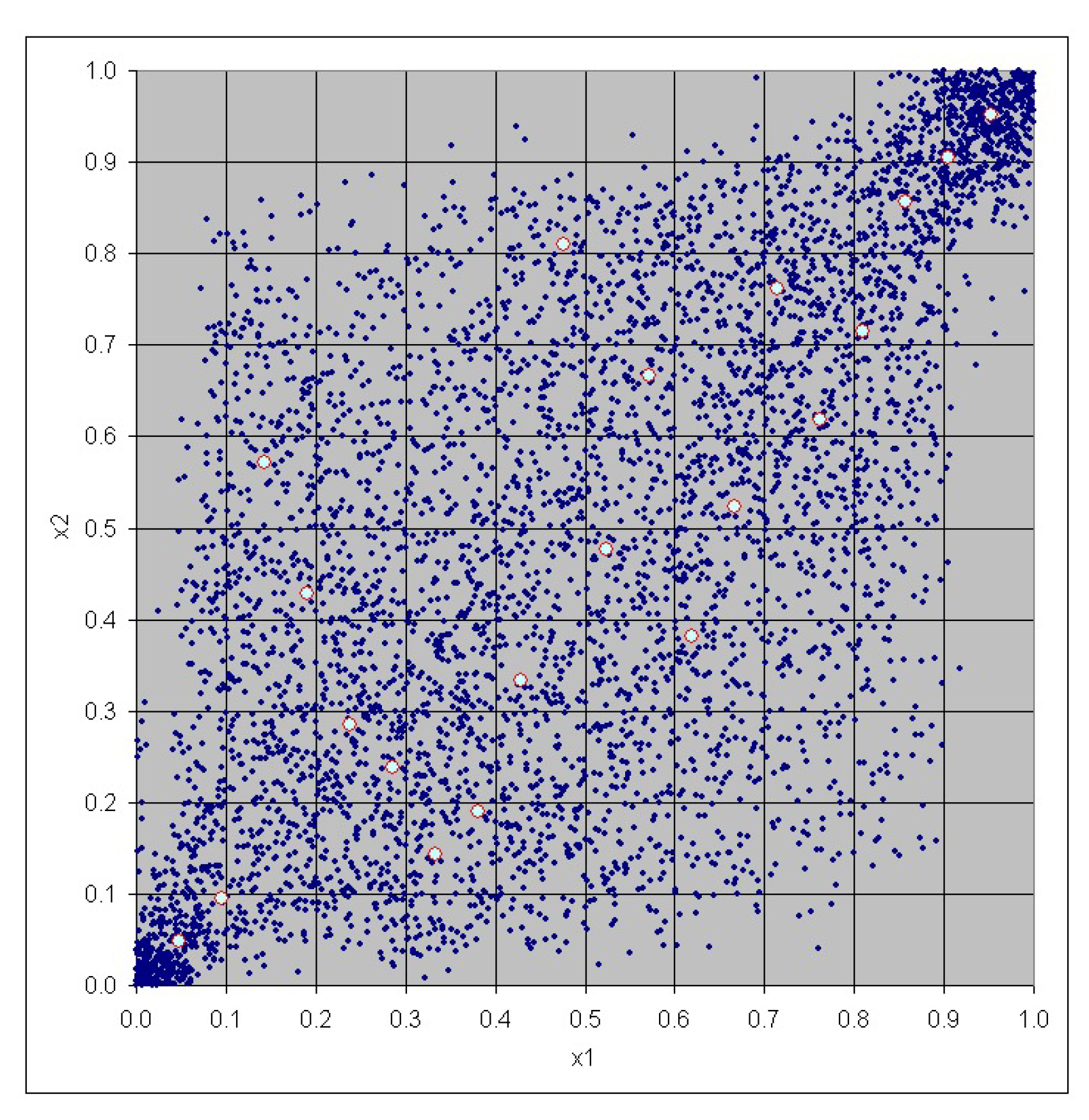
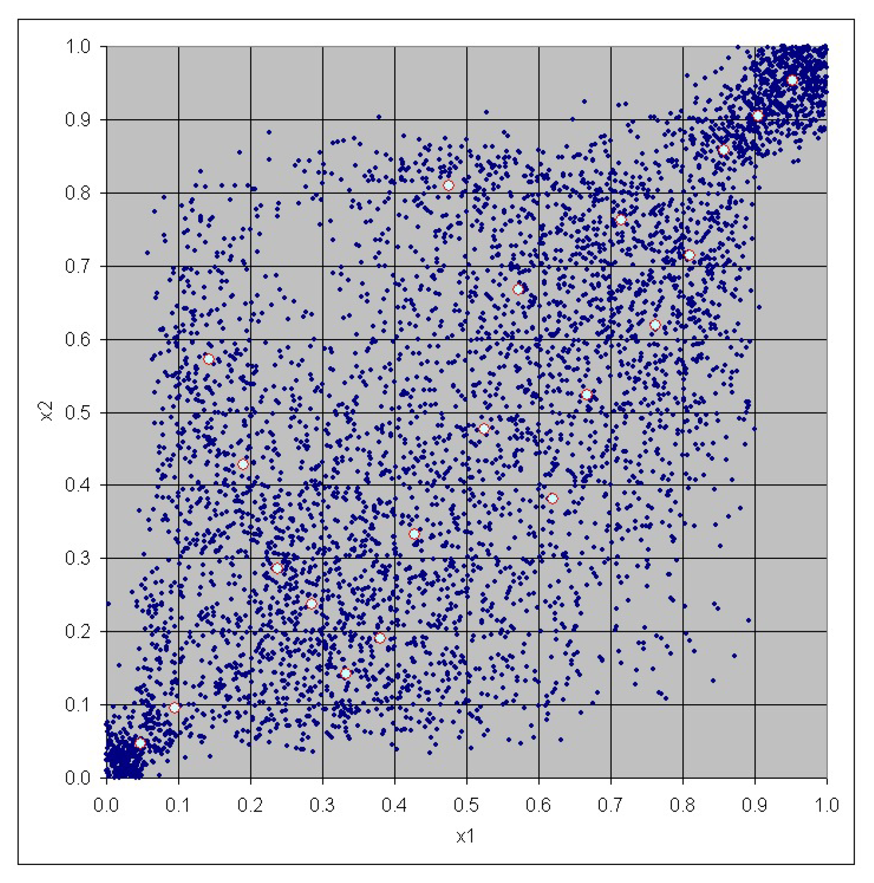
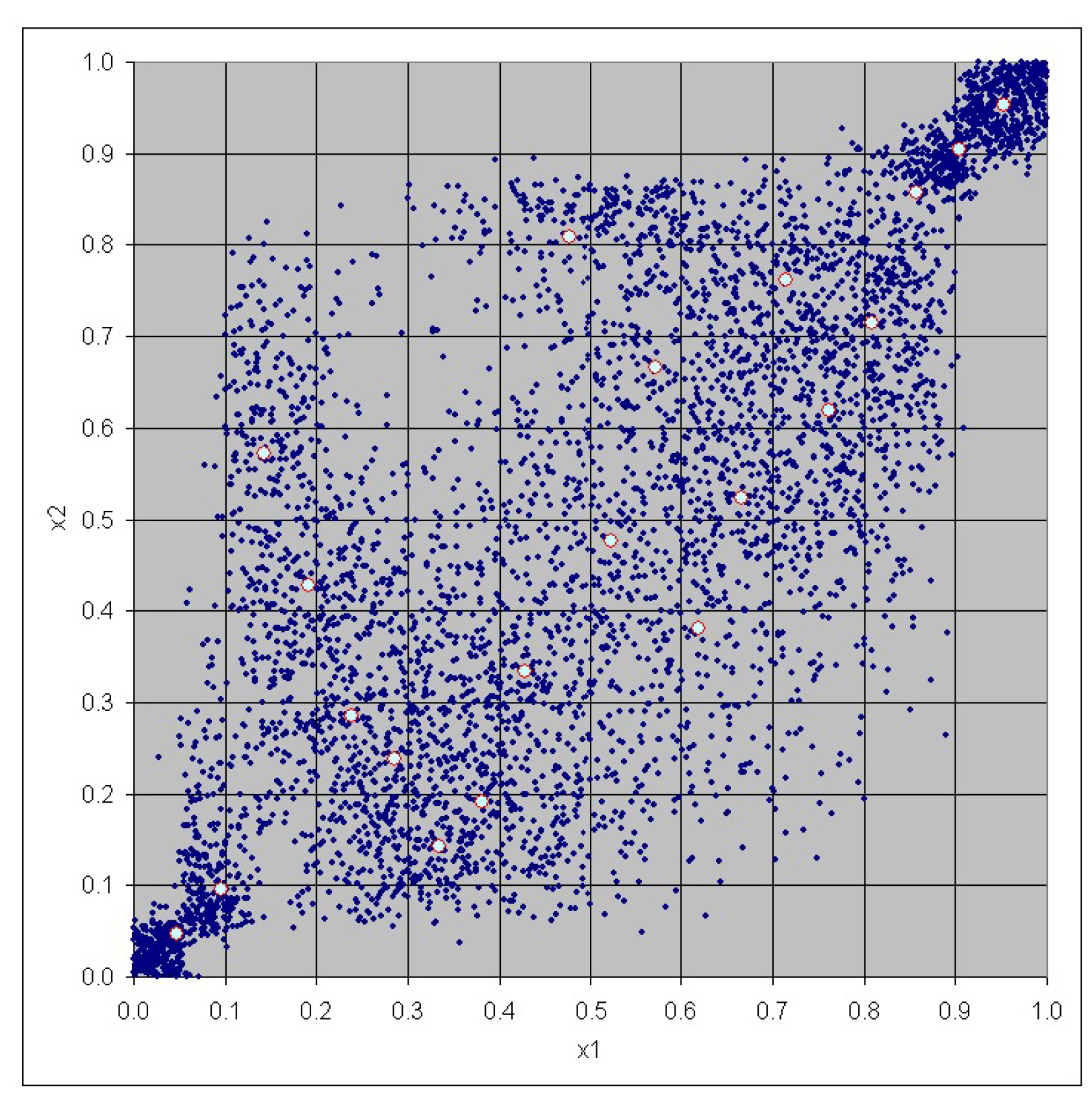
2. The Monte Carlo Algorithm

The central idea in this paper is to transform firstly n marginal observations from d different risks with suitably estimated cumulated distribution functions (cdf’s), so that the resulting data can be considered as observations from a multivariate distribution concentrated on the d-dimensional unit cube, similar—but typically not identical—to a copula. The next step is to approximate this distribution by a mixture of product beta distributions concentrated around each observation. This is similar to the estimation of the underlying dependence structure by a Bernstein copula or related constructions (see, e.g., Cottin and Pfeifer (2014) and Pfeifer et al. (2016, 2017, 2018)). By a marginal-wise backwards transformation of the simulated multivariate distribution with the quantile functions of the originally estimated marginal cdfs, we obtain realizations of an approximating distribution of the original data which allows for various VaR scenarios and VaR estimates that are particularly suitable in Internal Models under Solvency II. Note that this procedure influences the modelled dependence structure as well as the marginal distributions of the risks involved.

To be more precise, assume that $X_{ki}$ is the ith observation of the kth risk, for $i\in \{1,\dots ,n\}$ and $k\in \{1,\dots ,d\}$. Then, if $F_k$ denotes the true underlying cdf of the kth risk, then obviously $\left\{\left(F_1(X_{1i}),\dots ,F_d(X_{di})\right)|i=1,\dots ,n\right\}$ is a sample of the true underlying copula by Sklar’s Theorem (cf. Durante and Sempi (2016), chp. 2). Now, if ${\widehat{F}}_k$ denotes a suitably estimated absolutely continuous cdf for the kth risk and ${\widehat{f}}_k$ its corresponding density, define

$$\widehat{h}(x_1,\dots ,x_d):=\frac{1}{n}{\displaystyle \sum _{i=1}^n\prod _{k=1}^d}b\left(x_k,(m+1){\widehat{F}}_k(X_{ki}),(m+1)\left(1-{\widehat{F}}_k(X_{ki})\right)\right)\mathrm{for}(x_1,\dots ,x_d)\in {(0,1)}^d$$

(1)

(mixture of randomized product beta distributions) and

$$\widehat{g}(y_1,\dots ,y_d):=\widehat{h}\left({\widehat{F}}_1(y_1),\dots ,{\widehat{F}}_d(y_d)\right)·{\displaystyle \prod _{k=1}^d}{\widehat{f}}_k(y_k)\mathrm{for}(y_1,\dots ,y_d)\in {\mathbb{R}}^d,$$

(2)

where $b(x,\alpha ,\beta ):=\frac{{\displaystyle x^{\alpha -1}{(1-x)}^{\beta -1}}}{{\displaystyle B(\alpha ,\beta )}}$ for $0<x<1$ and $\alpha ,\beta >0$ denotes the density of the Beta distribution with parameters $\alpha$ and $\beta$, $B(\alpha ,\beta ):={\int }_0^1{x}^{\alpha -1}{(1-x)}^{\beta -1}\mathrm{d}x$ denotes the corresponding Beta function, and $m>0$ is a further steering parameter of the model. This approach is similar to the construction of Cottin and Pfeifer (2014) and resembles a classical kernel density estimate for the dependence structure where the kernel is represented by product beta densities.

Note that, given $X_{ki}=z$, the expectation of the Beta distribution with parameters $(m+1){\widehat{F}}_k(z)$ and $(m+1)\left(1-{\widehat{F}}_k(z)\right)$ is ${\widehat{F}}_k(z)$ and its variance is $\frac{{\displaystyle {\widehat{F}}_k(z)\left(1-{\widehat{F}}_k(z)\right)}}{{\displaystyle m+2}}\le \frac{{\displaystyle 1}}{{\displaystyle 4(m+2)}}$.

Seemingly, $\widehat{g}$ is the randomized density of a multivariate distribution (scenario distribution) that “interpolates” the original observations of the risks under investigation. This follows by similar arguments as Joe (2015), pp. 8–9 or Durante and Sempi (2016), Remark 2.2.2 since, obviously, $\widehat{h}$ is the randomized density of a d-dimensional distribution with cdf $\widehat{H}$, and $\widehat{g}$ is the density of the cdf $\widehat{G}$ defined by

$$\widehat{G}(y_1,\dots ,y_d):=\widehat{H}\left({\widehat{F}}_1(y_1),\dots ,{\widehat{F}}_d(y_d)\right)\mathrm{for}(y_1,\dots ,y_d)\in {\mathbb{R}}^d.$$

(3)

Note that, due to the remark above, the additional parameter m influences essentially the shape of the density $\widehat{g}$ as the bandwidth does for kernel type density estimators. In general, we can conclude that $\widehat{g}$ is more strongly concentrated around the original observations the larger m is. Given the observations $X_{ki}=x_{ki}$, simulations following the cdf $\widehat{G}$ or the density $\widehat{g}$ can be created as follows:

• Choose an index I randomly according to a uniform distribution over $\{1,\dots ,n\}$.
• Generate independently d random variables $Z_1$, …, $Z_d$ where $Z_k$ follows a Beta distribution with parameters $(m+1){\widehat{F}}_k(x_{kI})$ and $(m+1)\left(1-{\widehat{F}}_k(x_{kI})\right)$ (product beta distribution).
• Set $Y_k:={\widehat{F}}_k^{-1}(Z_k)$.

Then, $(Y_1,\dots ,Y_d)$ represents a Monte Carlo sample from the desired multivariate scenario distribution.

Obviously, the shape of the density $\widehat{g}$ depends on m as well as on the estimation of the marginal risk cdf’s. Hence, large sets of scenarios can be generated to estimate the VaR or other risk measures from Monte Carlo studies that embed the original data in a suitable way.

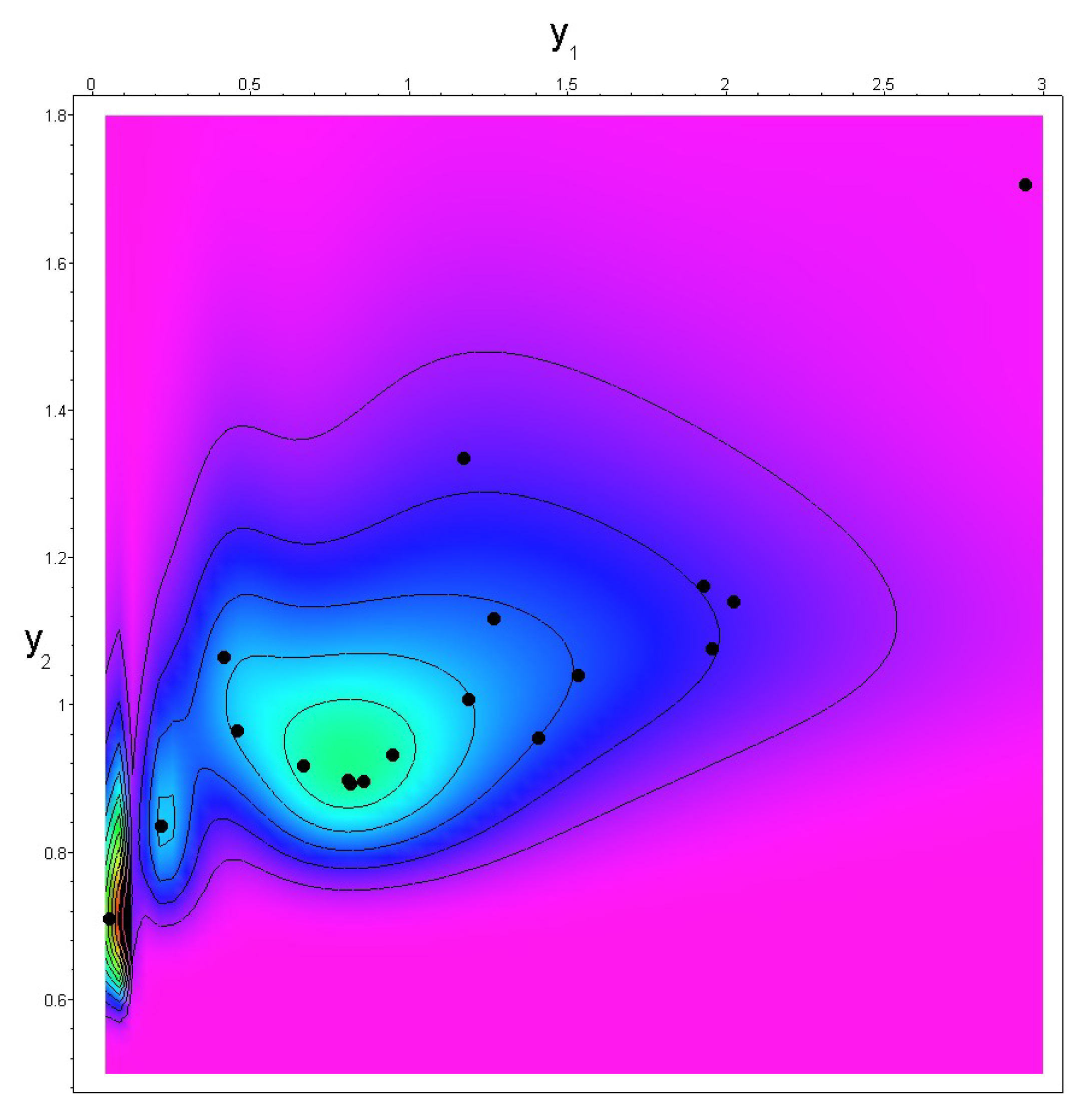
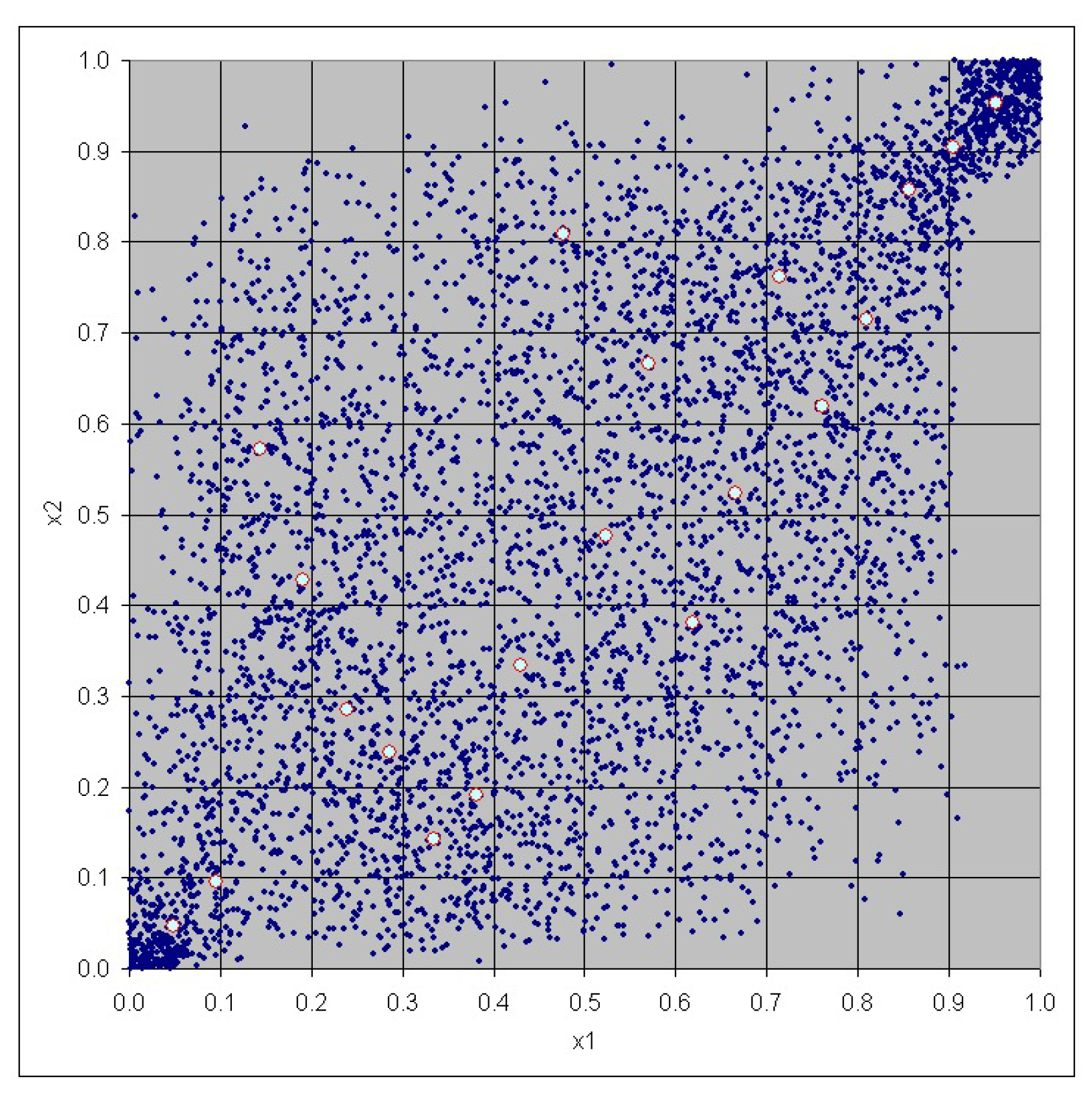
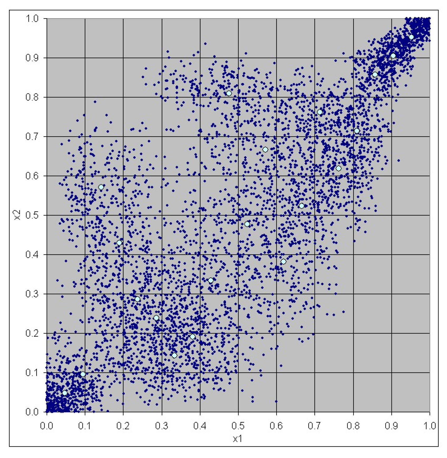
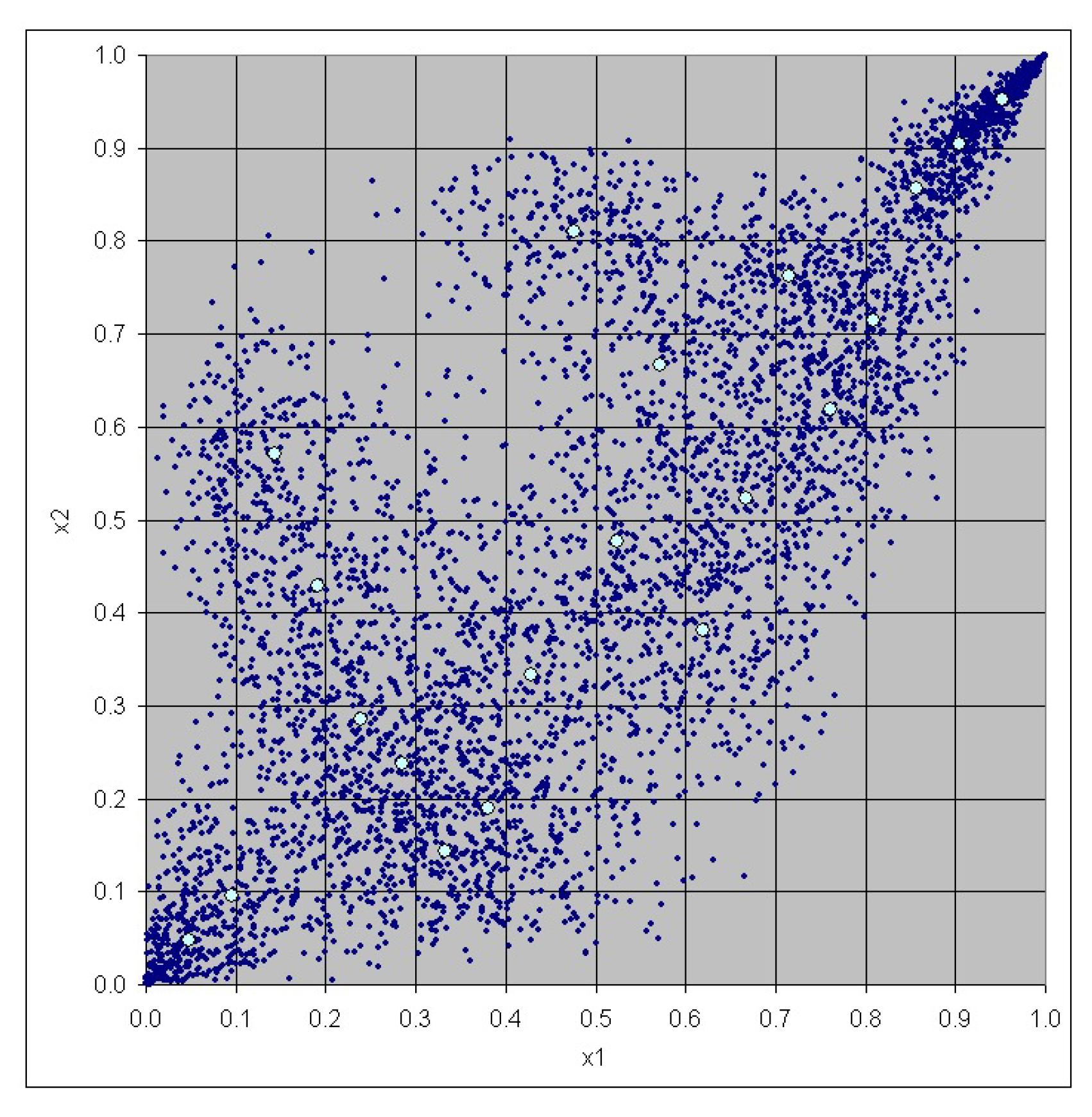
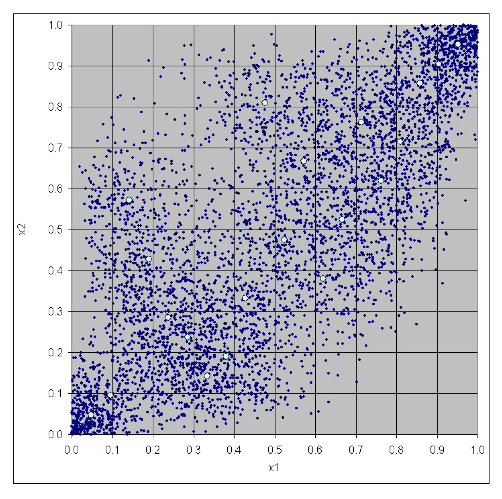
3. Case Study

For simplicity, we concentrate on the example data set given by Cottin and Pfeifer (2014) because it has also been used as a data basis in several papers on partition-of-unity copulas (Pfeifer et al. 2016, 2017, 2018). Here, we have $d=2$ and $n=20$. The marginal distributions were estimated by Q-Q-plots as normal and Gumbel for the log risks, i.e., as lognormal for the first risk and Fréchet for the second risk (see Table 1 and Figure 1 and Figure 2).

Table 1. The original data.

No.	Risk ${\mathit{X}}_1$	Risk ${\mathit{X}}_2$
1	0.468	0.966
2	9.951	2.679
3	0.866	0.897
4	6.731	2.249
5	1.421	0.956
6	2.040	1.141
7	2.967	1.707
8	1.200	1.008
9	0.426	1.065
10	1.946	1.162
11	0.676	0.918
12	1.184	1.336
13	0.960	0.933
14	1.972	1.077
15	1.549	1.041
16	0.819	0.899
17	0.063	0.710
18	1.280	1.118
19	0.824	0.894
20	0.227	0.837

Figure 1. Q-Q-plot for the first risk, log data.

Figure 2. Q-Q-plot for the second risk, log data.

From this analysis, we obtained estimates for the location parameter $\mu$ and the scale parameter $\sigma$ for the log risks (see Table 2).

Table 2. Parameter estimates for the log risks.

	$\mathit{\mu }$	$\mathit{\sigma }$
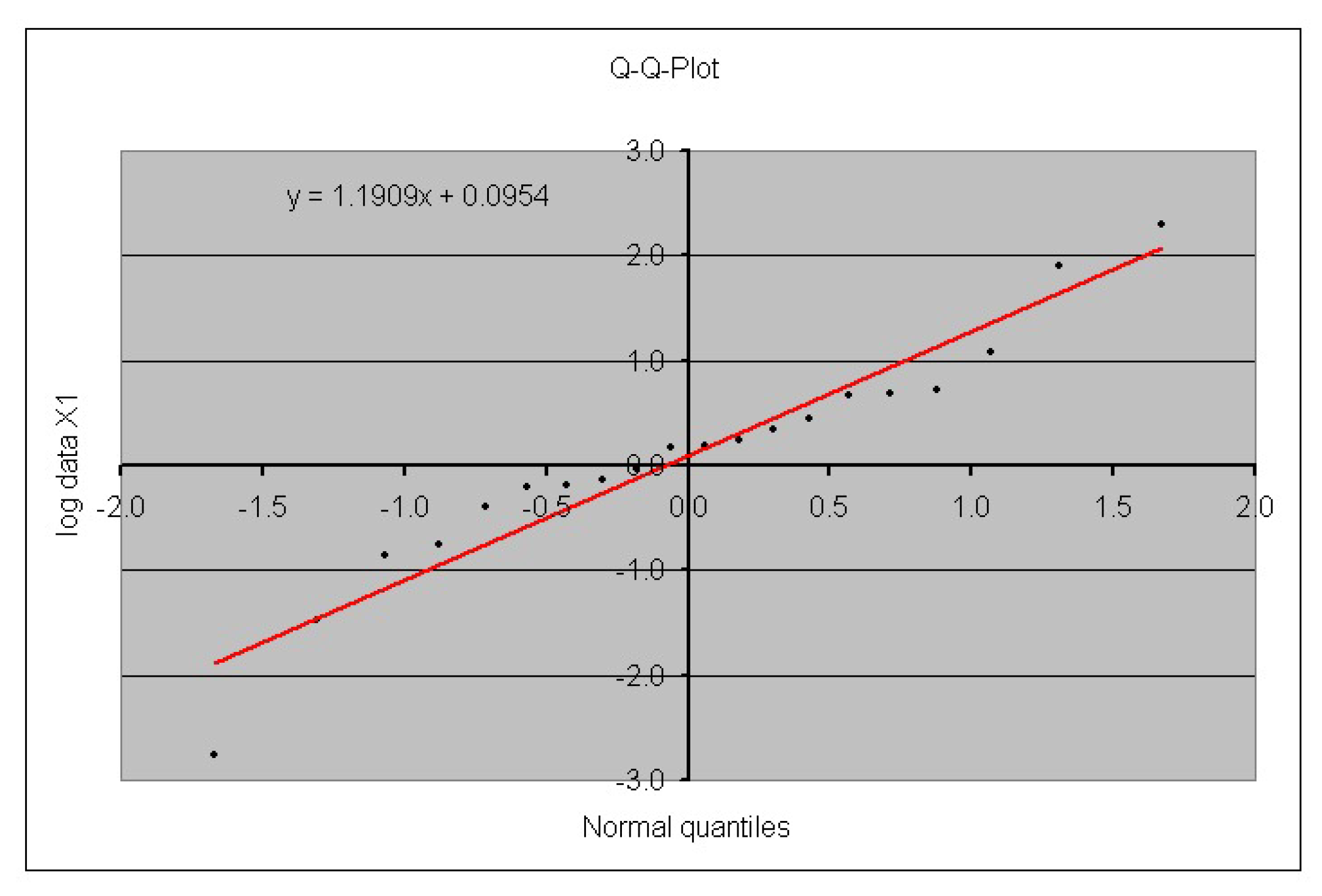
$ln(X_1)$	0.0954	1.1909
$ln(X_2)$	–0.0437	0.2857

The graphs in Figure 3, Figure 4, Figure 5, Figure 6, Figure 7, Figure 8, Figure 9, Figure 10, Figure 11, Figure 12, Figure 13 and Figure 14 show scatterplots for various Monte Carlo simulations with the algorithm described above, for several integer values of m, and graphs of the contour plots of the estimated scenario density $\widehat{g}$. The original data are marked by circles. The simulation size was 10,000 in each case. For comparison, we also present scatterplots for a Monte Carlo simulation with a certain adaptive kernel density estimator, where, for the first risk, we used pointwise lognormal densities and, for the second risk, Fréchet densities matching their modes with the data points (cf. Scott (2016), chp. 6.6). In particular, the kernel density estimator used here is given by

$$\widehat{f}(x,y,\sigma ,\alpha ):=\frac{1}{20}{\displaystyle \sum _{i=1}^{20}}{k}_1(x,X_{1i},\sigma )·k_2(y,X_{2i},\alpha ),$$

(4)

where

$$k_1(x,z,\sigma )=\frac{1}{\sqrt{2\pi }\sigma x}exp\left(-\frac{1}{2}{\left(\frac{ln\left(\frac{x}{z}\right)-{\sigma }^2}{\sigma }\right)}^2\right)$$

and

$$k_2(x,z,\alpha )=\frac{\alpha +1}{x}{\left(\frac{z}{x}\right)}^{\alpha }exp\left(-\left(1+\frac{1}{\alpha }\right){\left(\frac{z}{x}\right)}^{\alpha }\right),x>0.$$

Figure 3. Simulation scatterplot of $\widehat{g}(y_1,y_2)$, $m=15$. Small scale.

Figure 4. Simulation scatterplot of $\widehat{g}(y_1,y_2)$, $m=15$. Large scale.

Figure 5. Contour plot of $\widehat{g}(y_1,y_2)$, $m=15$.

Figure 6. Simulation scatterplot of $\widehat{g}(y_1,y_2)$, $m=30$. Small scale.

Figure 7. Simulation scatterplot of $\widehat{g}(y_1,y_2)$, $m=30$. Large scale.

Figure 8. Contour plot of $\widehat{g}(y_1,y_2)$, $m=30$.

Figure 9. Simulation scatterplot of $\widehat{g}(y_1,y_2)$, $m=50$. Small scale.

Figure 10. Simulation scatterplot of $\widehat{g}(y_1,y_2)$, $m=50$. Large scale.

Figure 11. Contour plot of $\widehat{g}(y_1,y_2)$, $m=50$.

Figure 12. Simulation scatterplot, kernel density estimate. Small scale.

Figure 13. Simulation scatterplot, kernel density estimate. Large scale.

Figure 14. Bivariate density contour plot, kernel density estimate.

For the kernel density estimate, the parameters $\sigma =0.3$ and $\alpha =7$ were used.

Table 3 shows various estimates of the ${\mathrm{VaR}}_{\alpha }$ for the aggregated risk (=$1-\alpha$-quantile of the sum distribution for the risks), calculated from 100,000 simulations each, where $\alpha$ denotes the risk level.

Table 3. VaR estimates for the aggregated risk.

	m = 15	m = 20	m = 25	m = 30	m = 50	m = 100	Kernel Density
${\widehat{\mathrm{VaR}}}_{0.05}$	13.987	12.978	12.347	12.016	11.341	10.908	11.754
${\widehat{\mathrm{VaR}}}_{0.01}$	40.637	31.235	26.989	23.966	19.498	16.580	17.272
${\widehat{\mathrm{VaR}}}_{0.005}$	60.752	44.270	36.410	30.846	23.390	18.864	19.087

Obviously, the estimated VaR’s decrease with increasing m for every risk level $\alpha$, which seems reasonable since, with increasing m, the scenario distribution is closer concentrated around the original data points, which is also clearly reflected in the graphs above. For $m\to \infty$, we would get a VaR estimate from the empirical distribution, i.e., a value of 12.630 for $\alpha \le 0.01$ and 8.980 for $\alpha =0.05$. Note also that with a kernel density approach, extreme scenarios can in general not be obtained.

It is interesting to observe that for $\alpha =0.005$ (Solvency II standard) the estimated VaR is almost twice as high for $m=15$ as in comparison to $m=30$.

VaR estimates with a classical Bernstein copula or finite, infinite or continuous partition-of-unity copulas with or without tail dependence as in Pfeifer et al. (2017, 2018) typically give much smaller values. Table 4 and Table 5 list some results for comparison. The rook copula driver for the Negative Binomial and the Gamma copula shows no tail dependence, while the upper Fréchet copula (UF) driver does. For technical details, see Pfeifer et al. (2017, 2018).

Table 4. VaR estimates with Bernstein and Negative Binomial copulas.

	Bernstein	NB Rook, a = 7	NB UF, a = 7	NB Rook, a = 15	NB UF, a = 15
${\widehat{\mathrm{VaR}}}_{0.05}$	7.166	6.885	7.016	6.974	7.155
${\widehat{\mathrm{VaR}}}_{0.01}$	15.634	15.973	15.744	15.877	16.059
${\widehat{\mathrm{VaR}}}_{0.005}$	21.105	20.801	21.311	20.256	21.733

Table 5. VaR estimates with Gamma copulas.

	Gamma Rook, a = 7	Gamma UF, a = 7	Gamma Rook, a = 15	Gamma UF, a = 15
${\widehat{\mathrm{VaR}}}_{0.05}$	9.330	10.072	9.522	10.191
${\widehat{\mathrm{VaR}}}_{0.01}$	18.113	21.224	18.550	21.428
${\widehat{\mathrm{VaR}}}_{0.005}$	22.933	28.123	23.079	28.588

The graphs in Figure 15, Figure 16, Figure 17, Figure 18, Figure 19, Figure 20, Figure 21, Figure 22 and Figure 23 show some realizations of the induced empirical copulas (scaled rank vectors) based on 5000 simulations for different choices of m and the kernel approach outlined above. The empirical copula of the original data (scaled rank vectors) is represented by circles in each plot. For comparison purposes, we also show some realizations of the Negative Binomial (NB) and the Gamma copulas using the parameters in Table 4 and Table 5, taken from Pfeifer et al. (2017, 2018) and Cottin and Pfeifer (2014).

Figure 15. Empirical copula, $m=15$.

Figure 16. Empirical copula, $m=30$.

Figure 17. Empirical copula, $m=50$.

Figure 18. Empirical kernel copula.

Figure 19. Gamma rook copula, $a=15$.

Figure 20. Gamma UF copula, $a=15$.

Figure 21. NB rook copula, $a=15$.

Figure 22. NB UF copula, $a=15$.

Figure 23. Bernstein copula.

Seemingly, the structure of the various copula approaches alone (with and without tail dependence) does not give any hint to the height of the VaR estimate for the aggregate risk. An ordering of the figures according to the decreasing magnitude of the VaR estimate for $\alpha =0.005$ (Solvency II standard) is: Figure 15, Figure 16, Figure 20, Figure 17, Figure 19, Figure 22, Figure 23, Figure 21, and Figure 18.

Finally, we present Q-Q-plots for the marginal distributions of the log risks from 5000 simulations for different choices of m and the kernel approach outlined above (see Figure 24 and Figure 25). The plot positions for the theoretical quantiles are chosen with the parameters from Table 2. Additionally, the original data points are shown as circles.

Figure 24. Q-Q-plot for the first risk, ordered log data.

Figure 25. Q-Q-plot for the second risk, ordered log data.

Seemingly, the product beta and the kernel density approach are in good coincidence with the body of the data, while the product beta approach is characterized by essentially higher values in the upper tail of the marginal distributions. This emphasizes again the fact that unfavourable VaR estimates cannot be characterized by the copula structure alone but that the interplay between the dependence structure and the marginal distributions is essential, as discussed by Ibragimov and Prokhorov (2017).

4. Conclusions

The algorithm proposed here typically generates mathematically well-defined high-score VaR scenarios on the basis of observed losses with particular emphasis on the underlying stochastic dependence which reproduce the original data exactly, and give stress tests and scenario analyses under Solvency II a more precise meaning. It is applicable in arbitrary dimensions and generally superior to kernel density or classical and recent copula approaches, with respect to complexity, easy implementation (even in usual spreadsheet programs), and larger scenario VaR estimates. We have tested the procedure described in this paper with the 19-dimensional dataset discussed by Neumann et al. (2018) and came to similar conclusions. A crucial point here is the estimation of the marginal distributions which, of course, influences the results to a certain extend, as does the value of m. However, in any case, the original data are exactly reproduced, and the selection of the steering parameters should depend on the purpose of the application.

References

- Blumentritt, Thomas. 2012. On Copula Density Estimation and Measures of Multivariate Association. Reihe: Quantitative Ökonomie 171. Lohmar: Eul Verlag. [Google Scholar]
- Cadoni, Paolo, ed. 2014. Internal Models and Solvency II. From Regulation to Implementation. London: Risk Books. [Google Scholar]
- Cherubini, Umberto, Elisa Luciano, and Walter Vecchiato. 2004. Copula Methods in Finance. New York: Wiley. [Google Scholar]
- Cottin, Claudia, and Dietmar Pfeifer. 2014. From Bernstein polynomials to Bernstein copulas. Journal of Applied Functional Analysis 9: 277–88. [Google Scholar]
- Cruz, Marcelo, ed. 2009. The Solvency II Handbook. Developing ERM Frameworks in Insurance and Reinsurance Companies. London: Risk Books. [Google Scholar]
- Durante, Fabrizio, and Carlo Sempi. 2016. Principles of Copula Theory. Boca Raton: CRC Press. [Google Scholar]
- Embrechts, Paul, Giovanni Puccetti, and Ludger Rüschendorf. 2013. Model uncertainty and VaR aggregation. Journal of Banking and Finance 37: 2750–64. [Google Scholar] [CrossRef]
- European Union. 2015. Commission Delegated Regulation EU 2015/35 of 10 October 2014 supplementing Directive 2009/138/EC of the European Parliament and of the Council on the taking-up and pursuit of the business of Insurance and Reinsurance (Solvency II). Official Journal of the European Union 17.1: L12/1–L12/797. [Google Scholar]
- Ibragimov, Rustam, and Artem Prokhorov. 2017. Heavy Tails and Copulas. Topics in Dependence Modelling in Economics and Finance. Singapore: World Scientific. [Google Scholar]
- Joe, Harry. 2015. Dependence Modeling with Copulas. Boca Raton: CRC Press. [Google Scholar]
- Mai, Jan-Frederik, and Matthias Scherer. 2017. Simulating Copulas. Stochastic Models, Sampling Algorithms, and Applications, 2nd ed. Singapore: World Scientific. [Google Scholar]
- Mainik, Georg. 2015. Risk aggregation with empirical margins: Latin hypercubes, empirical copulas, and convergence of sum distributions. Journal of Multivariate Analysis 141: 197–216. [Google Scholar] [CrossRef]
- Malevergne, Yannick, and Didier Sornette. 2006. Extreme Financial Risks. From Dependence to Risk Management. New York: Springer. [Google Scholar]
- McNeil, Alexander J., Rüdiger Frey, and Paul Embrechts. 2015. Quantitative Risk Management. Concepts, Techniques and Tools, 2nd ed. Princeton: Princeton University Press. [Google Scholar]
- Neumann, André, Taras Bodnar, Dietmar Pfeifer, and Thorsten Dickhaus. 2018. Multivariate multiple test procedures based on nonparametric copula estimation. Biometrical Journal, 1–22. [Google Scholar] [CrossRef] [PubMed]
- Pešta, Michal, and Ostap Okhrin. 2014. Conditional least squares and copulae in claims reserving for a single line of business. Insurance: Mathematics and Economics 56: 28–37. [Google Scholar] [CrossRef]
- Pfeifer, Dietmar, Andreas Mändle, Olena Ragulina, and Côme Girschig. 2018. Continuous partition-of-unity copulas and their application to risk management. Advances in Statistical Analysis. [Google Scholar]
- Pfeifer, Dietmar, Andreas Mändle, and Olena Ragulina. 2017. New copulas based on general partitions-of-unity and their applications to risk management (part II). Dependence Modeling 5: 246–55. [Google Scholar] [CrossRef]
- Pfeifer, Dietmar, Hervé Awoumlac Tsatedem, Andreas Mändle, and Côme Girschig. 2016. New copulas based on general partitions-of-unity and their applications to risk management. Dependence Modeling 4: 123–40. [Google Scholar] [CrossRef]
- Rank, Jörn, ed. 2007. Copulas. From Theory to Application in Finance. London: Risk Books. [Google Scholar]
- Rose, Doro. 2015. Modeling and Estimating Multivariate Dependence Structures with the Bernstein Copula. Ph.D. thesis, Lincoln Memorial University, München, Germany. [Google Scholar]
- Sandström, Arne. 2011. Handbook of Solvency for Actuaries and Risk Managers. Theory and Practice. London: CRC Press, Taylor & Francis Group. [Google Scholar]
- Schumaker, Larry L. 2015. Spline Functions: Computational Methods. Philadelphia: SIAM. [Google Scholar]
- Scott, David W. 2016. Multivariate Density Estimation. Theory, Practice, and Visualization, 2nd ed. Hoboken: Wiley. [Google Scholar]
- Szegö, Giorgio, ed. 2004. Risk Measures for the 21st Century. Chichester: Wiley. [Google Scholar]
- Yang, Jingping, Zhijin Chen, Fang Wang, and Ruodu Wang. 2015. Composite Bernstein copulas. ASTIN Bulletin 45: 445–75. [Google Scholar] [CrossRef]