1. Introduction
Research on futures hedging has been a popular topic in the agricultural economics literature. In particular, many studies have explored optimal hedge ratios for producers and the factors that influence their magnitude. Although academic studies generally support the use of futures hedging, anecdotal evidence suggests that few agricultural producers actually adopt futures contracts for hedging.
Peck and Nahmias (
1989) and
Collins (
1997) discuss how the disconnection between underlying assumptions of hedging models and hedgers’ decision context may explain why estimated and observed hedge ratios differ.
One of the factors often cited to explain why producers do not use futures contracts for hedging as much as suggested in academic studies are the transaction costs involved in a hedging operation. Previous studies have already indicated that the presence of transaction costs would typically reduce the optimal hedge ratio. For instance,
Lence (
1995,
1996),
Arias et al. (
2000) and
Mattos et al. (
2008) incorporate transaction costs in hedging models and find that optimal hedge ratios decrease as larger transaction costs are considered.
When previous studies incorporate transaction costs in hedging models, they typically consider fees charged by brokers or futures exchanges. Additionally, these fees are assumed to be deterministic, i.e., specific values that are fully known to hedgers at the beginning of the hedge. However, there are other transaction costs involved in futures hedging and the exact amounts of some of them are only known during or at the end of the hedge. Taxation and margin calls are two examples of this kind of transaction cost. The precise amounts to be paid in taxes or to be deposited in the hedgers’ margin account when there are margin calls that are unknown to hedgers when they start the hedge, because they depend on how much money is gained or lost in the futures market during the hedging period (i.e., they depend on the trajectory of futures prices during the hedge). This creates another dimension in the risk profile of a futures hedge, which is the notion of “cost risk”. This idea has not yet been explored in the literature and implies that a portion of transaction costs involved in futures hedging is stochastic.
The objective of this paper is to explore the notion of “cost risk” in futures hedging. An expected utility framework will be adopted in this study, with Monte Carlo methods used to simulate different price trajectories and their respective hedging costs. The uncertainty associated with hedging costs will be incorporated as an additional source of risk in the expected utility model, where a hedger’s trade-off between return and risk will be discussed. Hence, optimal hedge ratios will be simulated in the presence of a broader and more realistic set of transaction costs, which are stochastic in nature. The simulation will be based on a livestock producer in Brazil, who uses futures contracts on live cattle traded at the Brazilian futures exchange to hedge cattle sales.
Results from this study will improve our theoretical understanding of the risks involved in futures hedging and their influence in the determination of optimal hedge ratios. The simulation based on realistic conditions faced by a livestock producer will illustrate our theoretical discussion and provide further insights on hedging decisions by agricultural producers. Findings can be useful for producers (hedgers), marketing advisors, government, and futures exchanges, as it will allow them to understand better all risks involved in futures hedging and help them improve hedging strategies, design of contracts and regulations related to risk management.
2. Previous Studies
Several studies have investigated futures hedging under different conditions and explored factors that influence the demand for hedge by agricultural producers. Previous research has explored how optimal futures hedge ratios may vary in the presence of price risk, inefficient futures markets, production risk, basis risk, production diversification, producer’s risk aversion, other available marketing contracts, and producer’s limited knowledge about futures markets (e.g.,
Robison et al. 1984;
Hirshleifer 1988;
Lence 1995;
Hardwood et al. 1999;
Frechette 2000).
The impact of transaction costs on hedging decisions has also been largely explored in many studies. Since there are costs involved in futures trading, the benefits of futures hedging can be partially or completely outweighed by these transaction costs. For example,
Ennew et al. (
1992),
Collins (
1997),
Pannell et al. (
2008) and
Wolf (
2012) show how transaction costs reduce the attractiveness of futures hedging for producers. However, previous studies focus only on a few costs involved in futures hedging. Further,
Andrade (
2004) discussed a large set of costs that can affect the decision to use futures contracts to hedge, which are divided into six categories.
- (a)
Learning cost. This cost corresponds to the time and effort invested into learning how futures markets and hedging work.
- (b)
Exchange and brokerage fees. This is the most frequently addressed cost in the literature, and refers to the fees charged by the futures exchanges and brokerage houses for the execution of trades in the futures market.
- (c)
Liquidity cost. This one refers to the cost of entering and exiting the market, and is closely related to the trading volume in a given futures contract. The bid-ask spread is commonly used to measure this cost.
- (d)
Position management. When hedgers trade futures contracts, they need to dedicate time to monitor and manage their position in the futures market or pay someone to do so. Either way, there is a cost associated with the management of their position.
- (e)
Initial margin deposit. The margin system in the futures market requires that all traders make an initial margin deposit when they first trade a contract. Hence, there is an opportunity cost of having funds tied to the margin system.
- (f)
Margin calls. Traders can receive margin calls if the positions in the futures market start losing money. Hence, traders need to set aside some funds in order to meet those margin calls, which also corresponds to an opportunity cost.
- (g)
Taxation. If traders make a profit in the futures market, they have to pay taxes on their earnings. Although specific tax regulations can vary across different countries, this can be seen as another cost involved in futures trading.
Andrade (
2004) also discussed the stochastic nature of some costs. More specifically, costs associated with margin calls and taxation are unknown at the beginning of the hedge, because they depend on the evolution of the futures price during the hedging period. Thus, the stochastic behavior of futures prices generates a stochastic behavior for the margin calls and taxation faced by hedgers.
Andrade (
2004) refers to this uncertainty as “cost risk”, which can be modelled with probability distributions. However, it is not explored empirically how this idea of “cost risk” may affect hedging decisions.
In general, two approaches have been adopted to investigate futures hedging in the literature: Econometric methods and the expected utility framework. Econometric estimation is used to generate minimum variance hedge ratios. Although the econometric techniques adopted in those studies are fairly sophisticated,
Lence (
1995) highlights some limitations of the models based on a minimum variance hedge ratio. For example, those models do not account for transaction fees and margin calls, and neglect that fact that a given hedge ratio might not actually be traded due the standard size of futures contracts. Further, it is also assumed that hedgers do not have investments in other activities and do not borrow money in the market. Those limitations can be addressed in an expected utility framework, which focuses on optimal hedge ratios that maximize the hedger’s expected utility and was initially adopted in the study of hedging models by
Stein (
1961) and
Johnson (
1960)
1.
Arias et al. (
2000) adopted the expected utility framework to find optimal hedge ratios considering that producers’ “motivations to hedge are to reduce tax liabilities, bankruptcy costs, borrowing costs, and liquidity costs.” (
Arias et al. 2000, p. 392). In this context, they account for specific issues that can affect a producer’s decisions, such as the ability to borrow money, taxes associated to the hedge, the availability of funds to meet margin calls, and the existence of transaction fees to trade futures contracts. They found that optimal hedge ratios around 0–10% and argued that these numbers are consistent with observed hedging practices among agricultural producers. Despite the extensive analysis of how financial variables affect hedging decisions, they do not account for the stochastic nature of costs involved in futures hedging.
Lien and Li (
2003) introduced the discussion of how margin calls affect hedging decisions in their analysis. They argued that hedgers would consider large daily price changes (which could lead to margin calls and hence cash flow issues for producers) in their hedging decisions and would then reduce their hedging positions if they believed that those daily price changes were excessive. The authors stated that the “risk” associated with large margin calls was not typically addressed in the literature and claimed that this factor could discourage producers from hedging with futures contracts. Their results show that optimal hedge ratios are reduced when margin calls are taken into account in hedging decisions. Although they extensively discuss the possible impacts of margin calls on hedge ratios, their model is limited to margin calls and does not account for other types of transaction costs commonly incurred in hedging operations.
Wong and Xu (
2006) and
Adam-Müller and Panaretou (
2009) built on this idea and discussed “liquidity risk” in futures hedging. They discussed the case of producers/firms that use futures contracts to manage (output) price risk and may face losses in their futures position during the hedge. As the hedgers receive margin calls, there is the cost of additional funds that need to be used to meet margin calls. Both studies found that the presence of “liquidity risk” tends to reduce hedge ratios and may even lead to early liquidation of the hedge. Then they proposed the combination of futures and options contracts in those hedges as a way to attenuate the “liquidity risk”, but this point goes beyond the scope of the current research. Again, these two studies are limited to margin calls and do not account for a broader set of hedging costs.
Similar ideas were also addressed from different perspectives in
Acharya et al. (
2013) and
Brunetti and Reiffen (
2014), who explored trading in futures markets and hedging costs. They developed equilibrium models in which speculators are liquidity providers to hedgers.
Acharya et al. (
2013) focused on capital constraints (arising for margin requirements, for example) on the speculators’ end. These constraints would lead to limits to arbitrage between equity and commodity markets, which in turn would affect commodity futures prices and reduce hedging activity.
Brunetti and Reiffen (
2014) investigated whether trading by commodity index traders would affect the cost of hedging in commodity futures markets. Although they do not account for transaction costs explicitly, they do incorporate the idea that the volatility of futures prices impact hedging costs. Their general conclusion is that index traders provide hedging opportunities for commodity producers and can help reduce hedging costs compared to markets in which there are no index traders.
Transaction costs have also been explored when hedgers are not commodity producers and become particularly important when frequent trading is needed during the hedge. For example,
Jitmaneeroj (
2018) addressed the use of commodities in hedging stock portfolios and investigated the role of transaction costs in portfolio rebalancing (and hence hedge rebalancing). The study focused on the transaction cost per hedging effectiveness ratio to discuss whether the extra transaction costs involved in portfolio rebalancing would be compensated by higher hedging effectiveness. The findings varied according to the rebalancing horizon, indicating that transaction costs can have a major impact on hedging decisions. Similar idea was raised by
Wang et al. (
2015), who explored different hedging strategies with futures contracts compared to the naïve hedging. Their conclusion was that the naïve hedge generally performs better than other strategies before accounting for transaction costs. Although they did not incorporate transaction costs in the analysis, they claimed that naïve hedging would perform even better than other strategies (especially the ones with time-varying hedge ratios, which involve frequent rebalancing) if transaction costs were considered.
Overall, the standard conclusion from previous studies is that futures contracts become less attractive as a hedging tool when transaction costs are considered in the analysis. However, those studies generally include just a subset of costs involved in futures hedging and fail to consider costs that may have a major role in hedging decisions (e.g., income tax on futures and spot positions). Just as importantly, previous research has failed to fully account for the stochastic nature of some of those costs and how they can change the traditional discussion about hedging costs. As new stochastic variables are incorporated in the hedging model to reflect the nature of some transaction costs, new dynamics can emerge from the relationship between spot prices, futures prices and transaction costs, providing new insights on the role of transaction costs in hedging decisions. In the present study, a more realistic set of transaction costs will be adopted in the hedging model and the uncertainty associated with some transaction costs will also be incorporated. A more detailed discussion of the hedging model is provided in the next sections.
3. Transaction Costs in Brazil
The hedging simulation will be based on a livestock producer in Brazil, and two sets of transaction costs are considered. First, producers have to pay income tax on gains in their spot position. If a producer indicates a profit with his cattle business when taxes are filed, he has to pay a tax rate of up to 27.5% (the exact rate varies according to the magnitude of profit). Income tax is the only cost related to the spot market considered in this study. Although it is not directly associated with the hedging operation, it affects the dynamics between spot and futures prices in the hedging model (as will be discussed later).
A second set of transaction costs is associated with trading futures contracts, which comprises taxes, margin costs (daily mark-to-market), and exchange fees. Income tax is charged from producers on their monthly gains in their futures positions. At the end of each month, producers are charged an income tax rate of 15% on any gains they might have in their futures position. Note that these taxes apply to futures positions, which is separate from the income tax applied to the producer’s spot position. Margin costs refer to possible margin calls when the daily balance of producer’s margin account drops below the maintenance margin when accounts are marked-to-market every day. This cost can be viewed as either the borrowing cost of raising extra funds or the opportunity cost of using own funds to meet the margin calls. Finally, a third component of transaction costs in futures trading are exchange fees. Producers who trade futures contracts at the Brazilian Securities, Commodities and Futures Exchange (BM&FBOVESPA) have to pay four types of fees: Exchange/brokerage fees, settlement fees, permanence fees, and registration fees. Exchange fees account for the trading service provided by the exchange and depend on the total volume traded by the producer. Brokerage fees are charged by brokers but regulated by the futures exchange. Permanence fees are intended to cover operational costs incurred by the clearing house to keep track of hedgers’ positions and charged on a daily basis. Registration fees are also related to the clearing house and aim to cover expenses with registration service.
With respect to transaction costs related to futures trading, only exchange fees are fixed and thus known to hedgers by the time they place their hedges. Given the initial futures price on the day the hedge is placed, it is possible to calculate the total value of exchange/brokerage fees. On the other hand, income tax and margin costs are unknown to producers at the moment that they place their hedges. Producers might not need to pay income tax if their futures positions exhibit losses during the hedging period. If they do need to pay income tax, the actual value will depend on the magnitude of the gains in their futures position. Margin costs might also be zero if the balance of the producer’s margin account never falls below the maintenance margin. However, if they receive margin calls, the actual amount to be deposited in their margin accounts will vary according to the changes in futures prices.
4. Research Method
This study investigates how transaction costs and their stochastic nature affect optimal hedge ratios. Producers’ hedging decisions will be framed within an expected utility model and explored using a Monte Carlo simulation. In this section, we will discuss the variables adopted in the decision model and the procedures followed in the simulation.
The hedging decision of a producer in the presence of transaction costs will be investigated using an expected utility framework. It is assumed that a producer starts a short hedge with futures contracts in period
t = 0 and holds the hedge until period
t = 1, when his production is sold in the spot market and the futures hedge is terminated. The producer’s final wealth in period
t = 1 is given by
W1 as defined in Equation (1), where
W0 is initial wealth in period
t = 0,
S1 is the spot price in period
t = 1,
CP is the cost of production,
Q is the quantity produced and sold by the producer,
tax is the income tax rate on the spot position,
F0 and
F1 are the respective futures prices in periods
t = 0 and
t = 1,
h is the hedge ratio, and
TC is the total transaction cost involved in trading futures contracts.
An exponential utility function will be adopted to represent producer’s preferences and final wealth will be the argument of this function (Equation (2)). The parameter
α is the coefficient of absolute risk aversion. Since the return
R generated between periods
t = 0 and
t = 1 can be calculated by dividing final wealth by initial wealth (
R =
W1/
W0), final wealth can be expressed as
W1 =
W0R. Thus, return
R can be used as the argument of the utility function as in Equation (3), where
θ is the coefficient of relative risk aversion (
θ =
αW0).
If the probability distribution of return R is elliptically symmetric, then expected utility can be characterized by a function of the mean and variance of return
R (
Chamberlain 1983). In addition, when the return distribution is elliptically symmetric, then the distribution of final wealth satisfies the location and scale condition, which allows a two-parameter ranking of these risky alternatives to be consistent with an expected utility ranking (
Sinn 1983;
Meyer 1987). In this case, expected utility of return
R can be expressed in terms of its mean and variance as in Equation (4), where
µR and
are the mean and variance of the return distribution, respectively.
Since return is defined as
W1/
W0, Equation (1) can be algebraically manipulated such that
R is given by Equation (5), where
and
are the respective returns on the spot and futures positions,
tax is the income tax rate on the spot position,
h is the hedge ratio,
tc is the total transaction cost of trading futures contracts as a proportion of the initial futures price
and
. The mean and variance of
R are then given by Equations (6) and (7), where
µspot and
are the mean and variance of spot return distribution,
µfut and
are the mean and variance of the futures return distribution,
µtc and
are the mean and variance of the futures transaction cost distribution,
σspot,fut is the covariance between spot and futures returns,
σspot,tc is the covariance between spot returns and transaction costs, and
σfut,tc is the covariance between futures returns and transaction costs.
Substituting expressions (6) and (7) into (4), the optimal hedge ratio is determined by maximizing expected utility in (4) with respect to the hedge ratio
h. Assuming that spot returns are uncorrelated with transaction costs in futures trading (
σspot,tc = 0), the optimal hedge ratio is given by Equation (8). This expression will be used to calculate hedge ratios in the simulations performed in this study. Equation (8) incorporates the magnitude of transaction costs (
) as well as their stochastic nature (variance of transaction costs
, and covariance between transaction costs and futures returns
).
Assuming that the mean of futures returns is zero (
µfut = 0)
2, three hedge ratios can be discussed. First, in order to provide a benchmark for comparison, no transaction costs are assumed
. In this case, the optimal hedge ratio is simply the minimum-variance hedge ratio
. Given how returns are calculated, spot and futures returns are negatively correlated. Hence, the covariance between spot and futures returns is negative and the optimal hedge ratio is a positive number.
Next, deterministic transaction costs are considered, i.e., hedgers know exactly how much the costs are and hence there is no uncertainty related to transaction costs
. The optimal hedge ratio is then given by (9). The inclusion of positive mean transaction cost (
µtc) will reduce the magnitude of the numerator and thus lead to lower hedge ratios.
Finally, stochastic transaction costs are introduced, such that hedgers no longer know the exact amount of costs when they place the hedge. Now there is uncertainty related to transaction costs
and the optimal hedge ratio is given by (10). The positive mean transaction cost will again reduce the magnitude of the numerator, but the numerator will also change because of the variance of transaction costs (
) and the covariance between transaction cost and futures returns (
σfut,tc).
Equations (9) and (10) differ in their denominators, i.e., in the difference between variance of transaction costs and covariance between futures returns and transaction costs which appears in (10) but not in (9). If the variance of transaction costs is equal to the covariance between futures returns and transaction costs , then hedge ratios under stochastic costs in (10) will be the same as hedge ratios under deterministic costs in (9). If , then hedge ratios under stochastic costs in (10) will be lower than hedge ratios under deterministic costs in (9). Finally, if , then hedge ratios under stochastic costs in (10) will be higher than hedge ratios under deterministic costs in (9).
Therefore, when stochastic transaction costs are considered, optimal hedge ratios can increase or decrease (or even stay the same) compared to the case with deterministic transaction costs. It is not clear beforehand if the stochastic nature of transaction costs would make producers hedge more or less. The magnitudes of the variance of transaction costs and covariance between futures returns and transaction costs will determine the behavior of the optimal hedge ratio in the presence of stochastic costs.
Intuitively, stochastic transaction costs increase the total risk of the hedge, since the final price received by the producer (hedger) will be uncertain due to uncertainty in prices as well as uncertainty in transaction costs. If the variance of transaction costs is smaller than the covariance between futures returns and transaction costs , then trading futures contracts can also help “hedge” the variability in transaction costs. Therefore, when transaction costs are stochastic and , trading more futures contracts (i.e., higher hedge ratio) compared to the case of deterministic transaction costs will help hedge the total risk of the hedger. On the other hand, if the variance of transaction costs is greater than the covariance between futures returns (), then trading more futures contracts will actually increase the total risk of the hedge.
Finally, it will be assumed a coefficient of relative risk aversion (
θ) equal to 3 in this study. This is consistent with an average (or moderate) level of relative risk aversion discussed in the literature (e.g.,
Lence 1995;
Nelson and Escalante 2004).
5. Data
This research focuses on cattle producers who use futures contract to hedge in Brazil. Live cattle futures contracts in the Brazilian Securities, Commodities and Futures Exchange (BM&FBOVESPA) are traded for all 12 delivery months of the year, but the majority of the trading volume is concentrated in the May and October maturities. The last trading day of a contract is the last business day of the maturity month. The underlying commodity is an animal ready for slaughter with weight ranging between 450 and 550 kg (approximately between 990 and 1200 pounds). The futures contract size is 4950 kg (approximately 10,900 pounds), which corresponds to approximately 10 animals. Prices are quoted in the Brazilian currency–Reais (R$)–per 15 kg (about 33 pounds).
Two hedging horizons are considered: 2 months (42 trading days) and 4 months (84 trading days). The 2-month horizon corresponds to situations in which the producer decides to hedge the cattle price around the middle of the feeding cycle, while the 4-month horizon relates to cases when the hedge is placed at the beginning of the feeding cycle. Daily data on live cattle futures prices for the two most active delivery months–May and October–were collected from BMF&BOVESPA and used in this study to generate probability distributions for the two hedging horizons. Daily futures returns were calculated as , where p are daily futures prices. The annualized standard deviation (volatility) was calculated for each series of futures returns, and values ranged from 8.6% to 22.3%. Based on observed volatility, three values are selected to be used as parameters to generate a probability distribution of daily returns: 10%, 20%, and 30%. Round numbers are adopted for ease of exposition, and the first two values are chosen based on their proximity to the lowest and highest values calculated from the returns data. The last value was chosen to represent a scenario with higher uncertainty. The general behavior of futures returns and the values for means and variances are similar for both May and October contracts, so no distinction is made between delivery months. Data for these calculations were initially collected for the 2008–2012 period, but these values are also consistent with more recent data for live cattle futures returns in Brazil. Note that the goal is to generate probability distributions of returns (not prices) that are often observed in this market and commonly faced by cattle producers in Brazil.
Following
Lence (
1995) and
Mattos et al. (
2008), it is assumed that the expected return on futures contracts is zero (
µfut = 0). In fact, based on our data set, mean returns are not statistically distinguishable from zero. Assuming returns follow a normal distribution
, three probability distributions of futures returns are generated:
,
, and
, which are used to simulate futures price trajectories in each hedging horizon. For each probability distribution 5000 futures price trajectories are simulated for each hedging horizon. At this point, it was necessary to choose the same starting point for all price trajectories, which was set at the average price observed in the sample collected for this study (R
$90.00 per 15 kg). Each trajectory starts with
F0 = 90 and the second daily price is generated by randomly picking a daily return from the probability distribution and multiplying it by the initial price. The subsequent prices are also generated by randomly picking daily returns from the probability distribution and multiplying them by the price in the previous day. This process continues for 42 days in the 2-month hedging horizon and 84 days in the 4-month hedging horizon, and is repeated 5000 times for each probability distribution. At the end, there will be six sets of 5000 simulated futures price trajectories: 2-month hedging horizon with
, 2-month hedging horizon with
, 2-month hedging horizon with
, 4-month hedging horizon with
, 4-month hedging horizon with
, and 4-month hedging horizon with
.
The simulated price trajectories are used to calculate returns on spot and futures positions and transactions costs in each hedging horizon. It is assumed that spot and futures prices are the same on the last day of the hedging horizon (S1 = F1) and spot and futures returns are calculated as and , respectively. Cost of production (CP) used to calculate spot returns were obtained from the Center for Advanced Studies on Applied Economics (CEPEA). The set of spot and futures returns calculated from the 5000 trajectories are used to generate the covariance between spot and futures returns, which is then used to calculate the hedge ratios in (8)–(10).
Transaction costs in futures trading (as previously discussed) are also based on the price trajectories. Income tax on gains in futures markets and margin costs related to daily mark-to-market are calculated for each price trajectory and, in addition to the fixed exchange fees, are used to generate a probability distribution of transaction costs. Brazilian producers have to pay a 15% tax on net profits in futures trading at the end of every month. In the simulation, for each price trajectory, daily gains and losses in the producer’s futures position are calculated. At the end of each month, a 15% rate is applied if a net gain was observed. The expenses with income tax (Ctax) are calculated from all tax payments during the hedge. Opportunity costs are considered based on margin deposits required during the hedge. An interest cost of 11% (average rate observed in Brazil during the period in which prices were collected) is applied to the funds deposited by the producer during the hedge. The “margin cost” (Cmargin) is the sum of these costs during the hedge. Lastly, fees charged by brokers and futures exchanges are also considered in the calculation of transaction costs. Consistent with values charged from Brazilian hedgers, a fixed rate of 0.3% of the contract value is used to represent expenses with brokerage and exchange fees (Cfees). The total transaction cost TCi for each price trajectory i in each hedging horizon is calculated as TCi = Ctax,i + Cmargin,i + Cfees. Costs with income tax and margins will vary according to the price trajectory, while expenses with fees are the same for all trajectories.
Lastly, as discussed in Equation (5), transaction costs are adopted as a proportion of the initial futures price. The costs generated in each simulation yield a probability distribution for transaction costs, which allow calculating means (µtc) and variances () for transaction costs that are used to find the optimal hedge ratio in (8)–(10). Covariances between futures returns and transaction costs needed to calculate the hedge ratio in (8)–(10) are obtained from the simulated price trajectories.
Table 1,
Table 2 and
Table 3 show the means and standard deviations for total transaction costs and each one of the cot components. These values are based on the simulated price trajectories, hence income tax and opportunity costs associated with margin requirements depend on how futures prices behaved in each simulation. On the other hand, exchange fees are fixed and do not depend on the price trajectory. This is why standard deviations are positive for income tax and margin costs, and zero for exchange fees. In terms of magnitude, exchange fees represent a large portion of transaction costs in the scenario with lower price volatility (
Table 1). As higher price volatility is assumed in the simulated futures price trajectories (
Table 2 and
Table 3), income tax becomes more relevant to determine the total transaction cost.
Finally, as explained in a previous section, there is also income tax on producer’s spot position (producers have to pay 27.5% on profits from their cattle operation). This income tax does not depend on futures prices and therefore is not included in the transaction costs associated with the hedge. However, it is considered in the study because it affects the covariance between spot and futures returns. With this income tax, actual returns on the producer’s spot position are given by
, where
tax is the income tax rate on the profits of the cattle operation (if there is no profit, then
tax is zero). It can be shown that the covariance between spot returns (in the presence of income tax) and futures returns
is smaller than the covariance between those returns without income tax
(Equation (11)). As the income tax on producer’s spot position affects the covariance between spot and futures returns, it will impact the optimal hedge ratios calculated in (9) and (10).
6. Results
Results are initially discussed without transaction costs in futures trading, so that it is possible to assess the magnitude of hedge ratios without hedging costs. First, standard minimum-variance hedge ratios are calculated following Equation (8) and considering no costs either in the spot or futures positions
. Calculated ratios are presented in
Table 4 and values are close to 1 for both hedging horizons and all three scenarios for the volatility of futures prices. Income tax on spot positions is then introduced (
tax = 0.275), but there are still no transaction costs in futures trading. Hedge ratios drop to values between 0.71 and 0.79 as income tax is introduced for spot positions (
Table 4). This finding is expected because income tax affects the covariance between spot and futures returns, while there is no change in the variance of futures returns. As discussed in (11), this covariance becomes smaller when the tax rate of 0.275 is considered. Intuitively, it implies that changes in spot prices are not matched with changes in futures prices as closely as they would be without taxes on the spot position, hence making futures contracts relatively less effective.
Next, transaction costs in futures trading are considered. At first, these costs are included in a deterministic manner, i.e., there is a positive cost to trade futures contracts, but no uncertainty about the value of this cost
. Consistent with previous studies (such as
Lence 1995;
Mattos et al. 2008), the introduction of deterministic transaction costs in futures trading decreases the optimal hedge ratio. In the 2-month horizon, hedge ratios vary between 0 and 0.761 depending on the volatility scenario, while in the 4-month horizon they vary between 0.276 and 0.841 (
Table 5). Then, income tax on the spot position is also included with the deterministic transaction costs in futures trading, in which case there is a larger drop in optimal hedge ratios (
Table 5). In the scenario with lower volatility, optimal hedge ratios become zero for both hedging horizons when deterministic costs are considered for spot and futures positions.
Finally, uncertainty about transaction costs in futures trading is introduced. Now, in addition to a positive cost to trade futures contracts, producers also face uncertainty about the total value of these costs, which can only be known at the end of the hedge
. In line with findings discussed above and with previous studies, optimal hedge ratios when stochastic transaction costs in futures trading are introduced (
Table 6) are still smaller than hedge ratios that do not account for transaction costs in futures hedging (
Table 4). These results are consistent with the discussion in Equations (9) and (10) and show that a more realistic set of transaction costs faced by hedgers can substantially reduce the attractiveness of futures contracts as a hedging instrument.
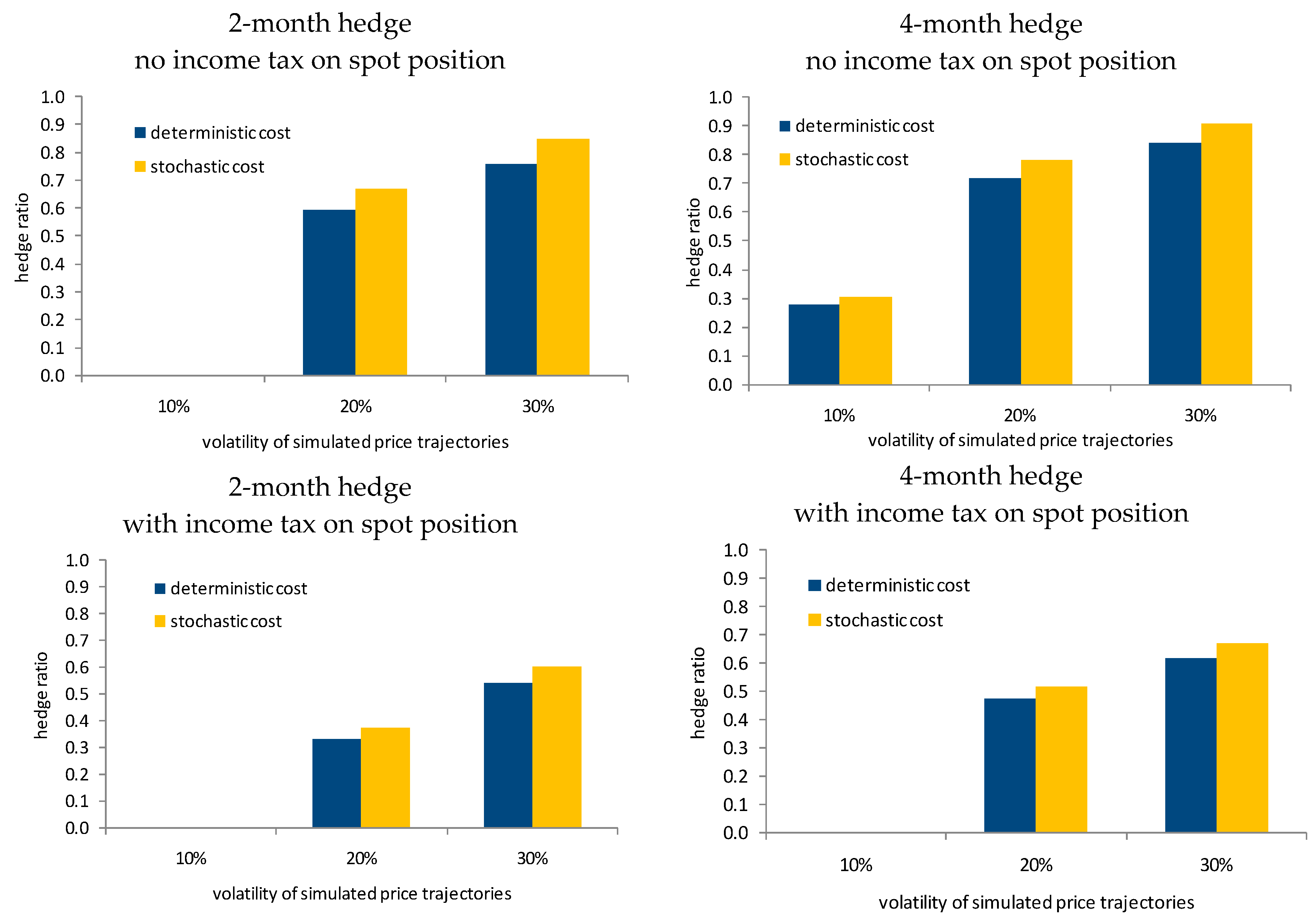
Another dimension of this study is the stochastic nature of transaction costs in futures trading. As shown in Equations (9) and (10), it is not theoretically evident whether considering stochastic transaction costs will increase or decrease optimal hedge ratios. In order to highlight the comparison of how uncertainty in transaction costs affects hedge ratios,
Figure 1 shows the same optimal hedge ratios as in the tables above, but now focusing on the differences between hedge ratios under deterministic transaction costs and under stochastic transaction costs. As can be seen, optimal hedge ratios increase when stochastic transaction costs are introduced compared to the cases with deterministic costs. This finding suggests that producers should trade a larger quantity of futures contracts when they are uncertain about the value of transaction costs, and a smaller quantity of futures contracts when they can determine the exact amount of transaction costs involved in their hedge. Based on our previous discussion, this is expected when the variance of transaction costs is smaller than the covariance between futures returns and transaction costs
, such that
in the denominator of Equation (10). In fact,
and
calculated from the simulations always show that
, which explains the findings in
Figure 1 and in the tables above.
7. Conclusions
Two main results emerge from this study. First, consistent with previous research (such as
Lence 1995;
Mattos et al. 2008;
Arias et al. 2000), the introduction of transaction costs in futures trading leads to smaller hedge ratios compared to scenarios without those costs. In the current study, a larger and more realistic set of transaction costs involved in futures trading was considered, along with income tax on producer’s spot position. Income taxes on both spot and futures positions represent a large portion of transaction costs associated with a cattle operation that uses futures contracts to hedge the price of its output in Brazil. Hence, it is important to understand the exact structure of transaction costs involved in futures hedging in a given market, and account for all relevant variables in the hedging model.
The second main finding of this study is that, if transaction costs are stochastic, it is not possible to determine beforehand how they will affect hedge ratios. This point brings new insights to the hedging literature and has not yet been extensively discussed. The actual value of income tax paid on futures positions and opportunity cost associated with margin requirements in futures markets depends on how the futures price changes during the hedging period. Therefore, before the hedge is placed, there is uncertainty about the total amount of transaction costs incurred in the hedge. Several futures price trajectories are simulated to assess the magnitude and variability of these two costs, which implies that hedgers also need to take into account the variability of transaction costs in their hedging decisions. Again, income tax on futures positions has a relevant role in the model, accounting for a large share of the total variability of transaction costs in futures trading. However, when optimal hedge ratios are calculated, uncertainty with transaction costs does not seem to have a large impact in this study (compared to the case of deterministic costs). In fact, the introduction of stochastic transaction costs in the hedging model causes optimal hedge ratios to increase slightly relative to the case with deterministic transaction costs. This result contrasts with
Arias et al. (
2000),
Lien and Li (
2003),
Wong and Xu (
2006) and
Adam-Müller and Panaretou (
2009), for example, who accounted for margin calls and liquidity constraints in futures hedging, but did not consider the stochastic nature of these costs.
In the current research, the impact of uncertainty in transaction costs on the optimal hedge ratio depends on the difference between the variance of transaction costs and the covariance between futures returns and transaction costs. In the current simulation, the variance of transaction costs is smaller than the covariance between futures returns and transaction costs, which increases hedge ratios when stochastic costs are considered. However, the covariance between futures returns and transaction costs depends on how transaction costs on futures trading are determined. Thus, it is possible that distinct results could be found in markets with different procedures to calculate transaction costs.
Further, the uncertainty in costs also affects the covariance between spot and futures returns. There are differences in income tax rates for the spot and futures markets, which imply that actual gains and losses in each market might not match as closely as it is usually considered in hedging studies. Therefore, the covariance between spot and futures returns would also be smaller than it is typically seen in hedging models.
The stochastic nature of costs in the hedging model creates a new dynamic between price returns and transaction costs that is important for practitioners. Previous studies have ignored the role of the covariance structure of price returns and stochastic costs, and the general findings in the literature are that larger costs lead to smaller optimal hedge ratios. Results from the current research show that this is not necessarily true. Depending on the covariance structure of price returns and stochastic costs, it is possible that larger costs lead to larger optimal hedge ratios. If hedgers do not account for this covariance structure, their hedge may actually be exposing them to more risk than previously thought. For example, the optimal hedge ratio for the 2-month hedging horizon in the scenario with 30% volatility is 0.539 when all costs are assumed to be deterministic (
Table 5) and 0.601 when the stochastic nature of those costs is accounted for (
Table 6). In this case, the producer would be under-hedged if costs were not properly considered in the analysis.
In summary, it should not be assumed that transaction costs in futures hedging automatically imply smaller optimal hedge ratios. Instead, an accurate set of hedging costs needs to be taken into account, along with the covariance structure between price returns and costs. The resulting analysis will then indicate whether hedging costs lead to smaller or larger optimal hedge ratios.
Finally, two points can be further explored in future research. One is the relationship between the variance of transaction costs and the covariance between futures returns and transaction costs, which makes hedge ratios increase in the presence of stochastic transaction costs in this study. As indicated above, transaction costs can be determined in many ways across futures markets and across countries, hence optimal hedge ratios may actually decrease in the presence of stochastic transaction costs depending on the values of the variance of transaction costs and the covariance between futures returns and transaction costs. Another point is how distinct income tax rates on the spot and futures positions impact the optimal hedge ratio. In the present model, tax rates on spot and futures positions are 27.5% and 15%, respectively. Different countries can have distinct tax structures. Since income tax accounts for a large portion of the mean and standard deviation of transaction costs in our model, results may vary considerably under distinct settings for income tax. It is even possible to investigate how alternative tax structures for spot and futures positions affect the trade-off between government revenue and the attractiveness of futures contracts as a hedging tool for commodity producers.


