Article

Robust Estimations for the Tail Index of Weibull-Type Distribution

by
Chengping Gong
1,† and
Chengxiu Ling
1,2,*,†
1
School of Mathematics and Statistics, Southwest University, Chongqing 400715, China
2
Department of Actuarial Science, University of Lausanne, Chamberonne, 1015 Lausanne, Switzerland
*
Author to whom correspondence should be addressed.
These authors contributed equally to this work.
Risks 2018, 6(4), 119; https://doi.org/10.3390/risks6040119
Submission received: 1 September 2018 / Revised: 30 September 2018 / Accepted: 9 October 2018 / Published: 11 October 2018
(This article belongs to the Special Issue Heavy-Tail Phenomena in Insurance, Finance, and Other Related Fields)

Abstract

:
Based on suitable left-truncated or censored data, two flexible classes of M-estimations of Weibull tail coefficient are proposed with two additional parameters bounding the impact of extreme contamination. Asymptotic normality with n -rate of convergence is obtained. Its robustness is discussed via its asymptotic relative efficiency and influence function. It is further demonstrated by a small scale of simulations and an empirical study on CRIX.

1. Introduction

The estimation of tail quantities plays an important role in extreme value statistics. One challenging problem is to select extreme sample fraction to balance the asymptotic variance and bias. Meanwhile, this requires a large and ideal sample from the underlying distribution. Indeed, in practical data analysis, it is not unusual to encounter outliers or mis-specifications of the underlying model which may have a considerable impact on the estimation results. A typical treatment is then required for instance by down-weighting its influence on the estimation in various standards, see e.g., Basu et al. (1998); Beran and Schell (2012); Vandewalle et al. (2004, 2007); Goegebeur et al. (2015); Liu and Tang (2010).
Given the wide applications of Weibull-type distributions and little studies on its robust estimations, this paper shall address this issue concerning its tail quantities. Let X 1 , , X n be an independent and identically distributed sequence from parent X F ( x ) satisfying
1 F ( x ) = exp { x α ( x ) } for   large   x ,
where α > 0 is the so-called Weibull tail coefficient (WTC) and ( x ) is a slowly varying function at infinity, i.e., (cf. Bingham et al. (1987))
lim t ( t x ) / ( x ) = 1 , x > 0 .
Prominent instances of Weibull-type distributions of F are Gaussian ( α = 2 ), gamma, Logistic and exponential ( α = 1 ) and extended Weibull (any α > 0 ) distributions (cf. Gardes and Girard (2008)). As an important subgroup of light-tailed distributions, Weibull-type distributions are of great use in hydrology, meteorology, environmental and actuarial science, to name but a few (cf. Arendarczyk and Dȩbicki (2011); Beirlant and Teugels (1992); Dȩbicki et al. (2018); Hashorva and Weng (2014)). Meanwhile, the WTC governs the tail behavior of F, and the larger the WTC is, the faster the tail of F decays. Dedicated estimations of WTC have thus been proposed and most of them are based on an asymptotically vanishing sample fraction of high quantiles, which asymptotic normality is achieved under certain second-order condition specifying the rate of convergence of ( t x ) / ( t ) to 1, see e.g., Girard (2004); Gardes and Girard (2008); Goegebeur et al. (2010); Asimit et al. (2010). Indeed, most data-sets from applied-oriented fields are relative large and with certain deviations from the pre-supposed model. For instance, it occurs with the slowly varying function ( · ) (where 1 F ( x ) = exp { x α ( x ) } ) in the left part of the distributions. To the best of our knowledge, it is new to investigate the robust Weibull tail estimations when only a small sample is available.
Inspired by the theory of robust inference in Huber (1964), we propose two classes of robust estimations of WTC. Denote for given c 0 > 0
h ( t ) = ( c 0 t 1 ) ln t 1 , t > 0 .
Clearly, we have g ( x ; α ) = α 1 h ( x α ) is the score function of
X F W ( x ; α ) = 1 exp { c 0 x α } , x > 0 , α > 0 .
Please note that h ( t ) , t > 0 is not monotone and thus one cannot directly weaken the effect of outliers by bounding score function g ( x ; α ) . On the other hand, most interest of risk management lies principally in the extreme large risks. This motivates us to consider some tailored h ( t ) according to certain left-truncated/censored Weibull distributions with the same Weibull tail coefficient α under considerations. Namely, we set below t 0 = arg min t 1 h ( t ) with h specified by (2) and
h ˜ ( t ) = h ( t ) , t 1 , h * ( t ) = h ( t ) , t t 0 ,
which properties are stated as below.
Lemma 1.
Let X F W ( x ; α ) and X ˜ = X | { X 1 } F ˜ W ( x ; α ) . Then h ˜ ( y ) = inf { t 1 : h ˜ ( t ) y } , y 1 is strictly increasing, and α 1 h ˜ ( x α ) is the score function of F ˜ W ( x ; α ) . Moreover, h * ( x α ) , x x 0 = t 0 1 / d 0 is strictly increasing provided that α d 0 > 0 .
Basically, both h ˜ and h * are certain modifications of h via its valued interval and domain region. Now, we are ready to state our M-estimations of Weibull tail coefficient using the M-estimation process based on the alternative samples X ˜ i ’s and X i * ’s respectively from X ˜ : = X | { X 1 } F ˜ and X * : = max ( X , x 0 ) F * where X i ’s is a random sample from X F . Set below [ y ] v u = min ( max ( y , v ) , u ) , } , v < u and is a set of distributions with support in ( 0 , ) .
Definition 1.
Let F W ( x ; α ) and h ˜ , h * be given by (3) and (4), respectively. Define the psi-function ψ ˜ as
ψ ˜ v , u ( y ; α ) = [ h ˜ ( y α ) ] v u 1 [ h ˜ ( z α ) ] v u d F ˜ W ( z ; α ) = [ h ˜ ( y α ) ] v u v + v u exp { c 0 [ h ˜ ( z ) 1 ] } d z , 1 v < u < .
Then the functional T ˜ ( F ) as the solution of the equation
λ ˜ F ( t ) = 1 ψ ˜ v , u ( y ; t ) d F ˜ ( y ) = 0 , F ,
is called huberized Weibull tail M-functional corresponding to ψ ˜ . The corresponding M-estimator T ˜ n = T ˜ n ( v , u ) ( F n ) , the solution of the equation
λ ˜ F n ( t ) = j = 1 m ψ ˜ v , u ( X ˜ j ; t ) = 0 , m = # { 1 i n : X i 1 } ,
is the huberized Weibull tail M-estimator of α. If further 0 < d 0 α d 1 , then define the psi-function ψ * with x 0 = arg min t 1 h ( t ) 1 / d 0 and v 0 = h ( x 0 d 1 )
ψ v , u * ( y ; α ) = [ h * ( y α ) ] v u x 0 [ h * ( z α ) ] v u d F W * ( z ; α ) = [ h * ( y α ) ] v u v + v u exp { c 0 ( h * ) ( z ) } d z , v 0 v < u < .
Then the functional T * ( F ) , F as the solution of the equation
λ F * ( t ) = x 0 ψ v , u * ( y ; t ) d F * ( y ) = 0 ,
is called huberized Weibull tail M-functional corresponding to ψ * . The corresponding M-estimator T n * = T n * ( v , u ) ( F n ) , the solution of the equation
λ F n * ( t ) = i = 1 n ψ v , u ( X i * ; t ) = 0 ,
is the huberized M-estimator of the Weibull tail coefficient α.
We remark that (5) and (6) hold since
F ˜ W ( x ; α ) = 1 exp { c 0 [ x α 1 ] } , x 1 ; F W * ( x ; α ) = 1 exp { c 0 x α } , x > x 0 , 0 , x x 0 .
Figure 1 illustrates the lower huberization by comparing the score function ψ ˜ 1 , ( y ; α ) of F ˜ W (recall Lemma 1) with ψ ˜ v , ( y ; α ) . We see that the contaminated Weibull density by Gamma (see (10) below for its definition) has almost the same shape as the pre-supposed Weibull one in the right tail, and therefore lower-huberized psi-function ψ ˜ v , ( y ; α ) can restrict the influence of all observations below y 0 = ( h ˜ ( v ) ) 1 / α instead of removing them completely. On the other hand, for all y > y 0 , the ψ ˜ v , ( y ; α ) is shifted downwards for the consistency purpose. One may similarly analyze the ψ * function.
The paper principally investigates the asymptotic behavior of the proposed new classes of M-estimations of Weibull tail coefficient. Details are as follows.
In Section 2, we consider Weibull distributions in Theorems 1 and 2 and establish its asymptotic normality of the M-estimations T ˜ n and T n * with n -rate of convergence, which is rather faster than that of most classical Weibull tail estimations such as the Hill-type estimation, see Theorem 2 in Girard (2004). Generally, we study related asymptotic properties in Theorems 3 and 4 when the underlying risk follows Weibull-type distributions specified in (1). Some bounded asymptotic bias may appear due to its deviations from the Weibull distributions.
In Section 3, using asymptotically relative efficiency (AEFF) and influence function (IF), we investigate the robustness (Theorem 5) and the bias, which are further related to the choices of flexible parameters v and u. These results are useful, especially when the practical regulators in risk management consider the trade-off between the robustness and consistency.
In Section 4, a small scale of Monte Carlo simulations and an empirical study concerning the CRIX proposed by Trimborn and Härdle (2016) are carried out. We see that both M-estimations are robust and perform very well even for small samples, in comparisons with the classical maximum likelihood estimations and Hill-type estimations of the Weibull tail coefficient. We expect the results would be beneficial to both financial practitioners and theoretical experts in risk management and extreme value statistics.
The rest of the paper is organized as follows. Main results are given in Section 2 followed with a section dedicated to the robust analysis. Section 4 and Section 5 are devoted to a small scale of Monte Carlo simulations and an empirical studies on CRIX. All proofs of the results are postulated to Section 6.

2. Asymptotic Results

Throughout this section, we keep the same notation as in Introduction and write further p and d for the convergence in probability and in distribution, respectively. All the limits are taken as n unless otherwise stated.
Theorem 1.
Let X 1 , , X n be a random sample from X F W ( x ; α 0 ) = 1 exp { c 0 x α 0 } , x > 0 , c 0 , α 0 > 0 . Denote by X ˜ j X ˜ = X | { X 1 } , 1 j m = # { 1 i n : X i 1 } , and by T ˜ n = T ˜ n ( v , u ) , 1 v < u < the solution of
λ ˜ ( F W ) n ( t ) = i = 1 m ψ ˜ v , u ( X ˜ i ; t ) = 0 .
Then T ˜ n p α 0 and
n ( T ˜ n α 0 ) d N ( 0 , σ ˜ v , u , α 0 ; F W 2 ) ,
where, with μ ˜ = v + v u exp { c 0 [ h ˜ ( z ) 1 ] } d z
σ ˜ v , u , α 0 ; F W 2 = e c 0 α 0 2 c 0 2 ( v μ ˜ ) 2 + 2 h ˜ ( v ) h ˜ ( u ) [ h ˜ ( s ) μ ˜ ] exp { c 0 ( s 1 ) } d h ˜ ( s ) h ˜ ( v ) h ˜ ( u ) s ln s exp { c 0 ( s 1 ) } d h ˜ ( s ) 2 .
Remark 1.
As stated in Lemma 1, α 1 h ˜ ( x α ) , x 1 is the score function of F ˜ W ( x ; α ) . Therefore, T ˜ n = T ˜ n ( v , u ) with v = 1 , u = reduces to the maximum likelihood estimation of α. This fact will be used in Theorem 5 for the asymptotic relative efficiency analysis. Additionally, we have by laws of large numbers that m = m ( n ) satisfies m / n p P { X 1 } = e c 0 .
Theorem 2.
Let X 1 , , X n be a random sample from X F W ( x ; α 0 ) = 1 exp { c 0 x α 0 } , x > 0 and 0 < d 0 α 0 d 1 . Denote by X i * = max ( X i , x 0 ) , 1 i n with x 0 = ( arg min t 1 h ( t ) ) 1 / d 0 , and by T n * = T n * ( v , u ) , n N , u > v v 0 = h ( x 0 d 1 ) the solution of
λ ( F W ) n * ( t ) = i = 1 n ψ v , u * ( X i * ; t ) = 0 .
Then T n * p α 0 and
n ( T n * α 0 ) d N ( 0 , σ v , u , α 0 ; F W * 2 ) ,
where, with μ * = v + v u exp { c 0 ( h * ) ( z ) } d z
σ v , u , α 0 ; F W * 2 = α 0 2 c 0 2 ( v μ * ) 2 + 2 ( h * ) ( v ) ( h * ) ( u ) [ h * ( s ) μ * ] exp { c 0 s } d h * ( s ) ( h * ) ( v ) ( h * ) ( u ) s ln s exp { c 0 s } d h * ( s ) 2 .
Remark 2.
(i) The difference between ψ ˜ and ψ * is that h * is not the score function of F W * , the distribution of the censored risk at point x 0 , where 0 < d 0 α 0 d 1 is needed to ensure the monotonicity of h * and ψ * , see details in (19) with α = α 0 .
(ii) The proposed M-estimations are principally based on suitable left-truncated and censored data, which are commonly used in survival analysis, see e.g., Kudu et al. (2017). Moreover, both consistency and robustness are obtained since we bound the psi-functions to weaken the influence of the extreme outliers for the exact Weibull models.
In what follows, we consider generally the Weibull-type risks and investigate asymptotic properties of the proposed M-estimations.
Theorem 3.
Let X 1 , , X n be a random sample from F ( x ) = 1 exp { c 0 x α 0 ( x ) } , x > 0 . Suppose that there is a unique solution t 0 of λ ˜ F ( t ) = 0 . Then T ˜ n = T ˜ n ( v , u ) , 1 v < u < , the solution of
λ ˜ F n ( t ) = i = 1 m ψ ˜ v , u ( X ˜ i ; t ) = 0 , m = # { 1 i n : X i 1 } ,
converges in probability to t 0 . If further 1 ψ ˜ v , u 2 ( x ; t 0 ) d F ˜ ( x ) < and λ ˜ F ( t ) 0 hold in a neighbourhood of t 0 , then
n ( T ˜ n t 0 ) d N ( 0 , σ ˜ v , u , t 0 ; F 2 ) ,
where
σ ˜ v , u , t 0 ; F 2 = e c 0 ( 1 ) 1 ψ ˜ v , u 2 ( x ; t 0 ) d F ˜ ( x ) [ λ ˜ F ( t 0 ) ] 2 .
Theorem 4.
Let X 1 , , X n be a random sample from F ( x ) = 1 exp { c 0 x α 0 ( x ) } , x > 0 and 0 < d 0 α 0 d 1 , x 0 = ( a r g m i n t 1 h ( t ) ) 1 / d 0 . Suppose that there is a unique solution t 0 of λ F * ( t ) = 0 . Then T n * = T n * ( v , u ) , u > v v 0 = h ( x 0 d 1 ) , the solution of
λ F n * ( t ) = i = 1 n ψ v , u * ( X i * ; t ) = 0 , n N ,
converges in probability to t 0 . If further x 0 ψ v , u * 2 ( x ; t 0 ) d F * ( x ) < and ( λ F * ) ( t ) 0 hold in a neighbourhood of t 0 , then
n ( T n * t 0 ) d N ( 0 , σ v , u , t 0 ; F * 2 ) ,
where
σ v , u , t 0 ; F * 2 = x 0 ψ v , u * 2 ( x ; t 0 ) d F * ( x ) [ ( λ F * ) ( t 0 ) ] 2 .
Please note that here the t 0 , the unique solution of λ ˜ F and λ F * specified in Theorems 3 and 4, might not be equal to α 0 . In other words, to maintain the robustness of the M-estimations is at cost of consistency. In the next section, we shall discuss the balance via the flexible parameters v and u.

3. Robustness

A simple criterion for choosing v and u in the M-estimations is the trade-off between the efficiency loss (that one is willing to put up with when data are generated by a Weibull distribution), and its asymptotic bias (when the underlying distribution deviates from the ideal Weibull distribution). We study below the relative asymptotic efficiency (AEFF) in Theorem 5, and then analyze its influence function. Both quantities are some functions of the flexible parameters v and u, which enable the risk regulators to balance the robustness and consistency.
As stated in Remark 1, the M-estimation T ˜ n ( v , u ) with v = 1 , u = reduces to the maximum likelihood estimation of α . Therefore, a straightforward application of Theorems 1 and 2 leads to the following theorem.
Theorem 5.
Under the same assumptions of Theorems 1 and 2, we have the relative asymptotic efficiency functions of T ˜ n ( v , u ) and T n * ( v , u ) (compared to T ˜ n ( 1 , ) , the maximum likelihood estimation) are given by
A E F F ( T ˜ n ( v , u ) ) = σ ˜ 1 , , α 0 ; F W 2 σ ˜ v , u , α 0 ; F W 2 = 1 exp { c 0 [ h ˜ ( z ) 1 ] } d z 2 + 2 1 [ h ˜ ( s ) μ ˜ ] exp { c 0 ( s 1 ) } d h ˜ ( s ) 1 s ln s exp { c 0 ( s 1 ) } d h ˜ ( s ) 2 × h ˜ ( v ) h ˜ ( u ) s ln s exp { c 0 ( s 1 ) } d h ˜ ( s ) 2 ( v μ ˜ ) 2 + 2 h ˜ ( v ) h ˜ ( u ) [ h ˜ ( s ) μ ˜ ] exp { c 0 ( s 1 ) } d h ˜ ( s )
and
A E F F ( T n * ( v , u ) ) = σ ˜ 1 , , α 0 ; F W 2 σ v , u , α 0 ; F W * 2 = e c 0 1 exp { c 0 [ h ˜ ( z ) 1 ] } d z 2 + 2 1 [ h ˜ ( s ) μ ˜ ] exp { c 0 ( s 1 ) } d h ˜ ( s ) 1 s ln s exp { c 0 ( s 1 ) } d h ˜ ( s ) 2 × ( h * ) ( v ) ( h * ) ( u ) s ln s exp { c 0 s } d h * ( s ) 2 ( v μ * ) 2 + 2 ( h * ) ( v ) ( h * ) ( u ) [ h * ( s ) μ * ] exp { c 0 s } d h * ( s ) .
Here μ ˜ and μ * are given by Theorems 1 and 2, respectively.
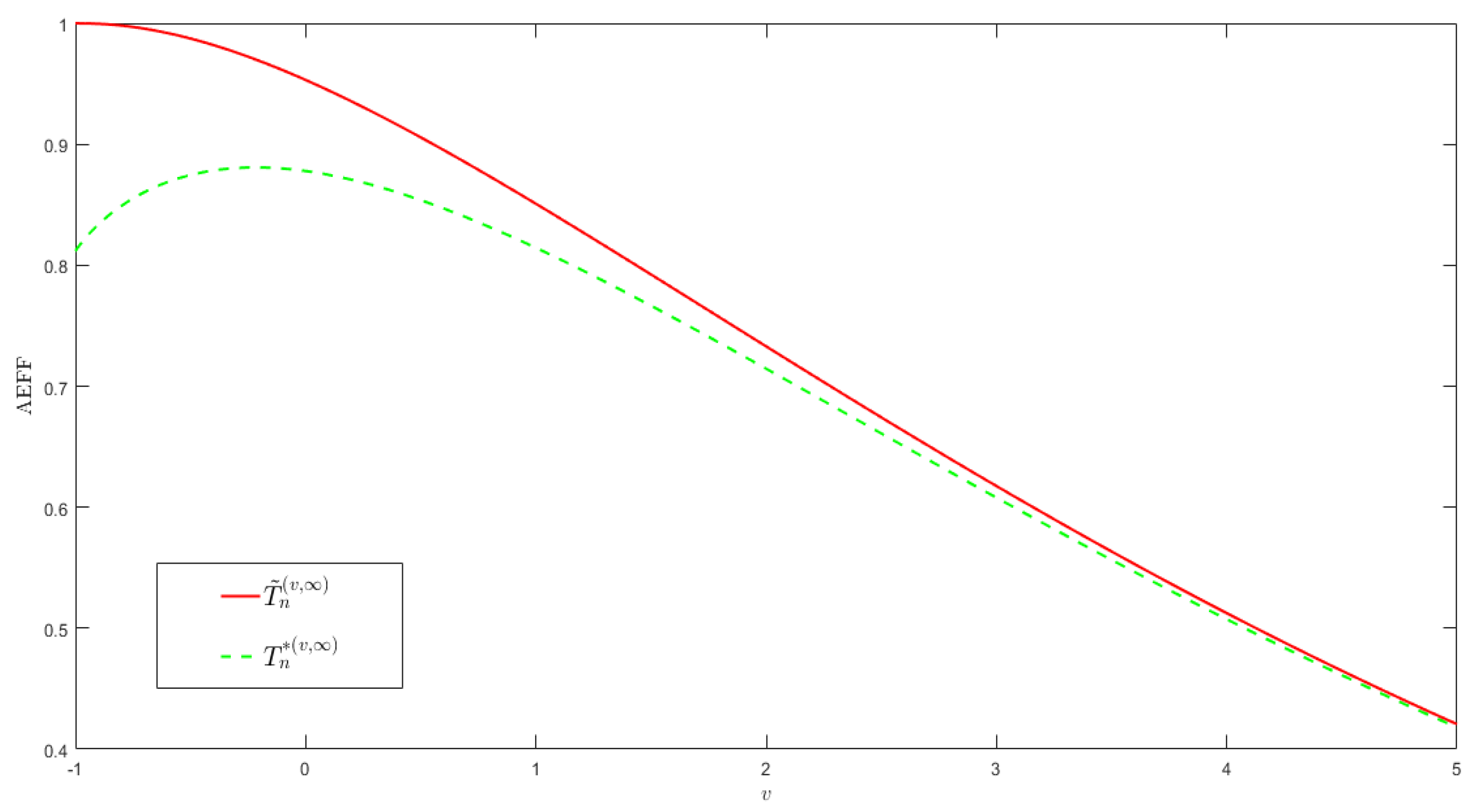
Figure 2 illustrates the effect of v on the relative asymptotic efficiency of T ˜ n ( v , ) and T n * ( v , ) (compared to the MLE T ˜ n ( 1 , ) ). For smaller v, the relative asymptotic effective loss of T ˜ n is rather smaller than that of T n * . While for larger v, both are asymptotically the same.
The influence function approach, known also as the “infinitesimal approach”, is generally employed to quantify robustness. Recall that the influence function describes the effect of some functional T ( F ) for F in an infinitesimal ϵ -contamination neighbourhood { F ϵ | F ϵ ( x ) = ( 1 ϵ ) F ( x ) + ϵ G ( x ) } , is defined by
I F ( T ; F , G ) = lim ϵ 0 T ( ( 1 ϵ ) F + ϵ G ) T ( F ) ϵ = ϵ T ( F ϵ ) | ϵ = 0 .
We have
I F ( T ˜ ; F , G ) = 1 ψ ˜ v , u ( y ; T ˜ ( F ) ) d G ˜ ( y ) λ ˜ F ( T ˜ ( F ) ) ; I F ( T * ; F , G ) = x 0 ψ v , u * ( y ; T * ( F ) ) d G * ( y ) ( λ F * ) ( T * ( F ) ) .
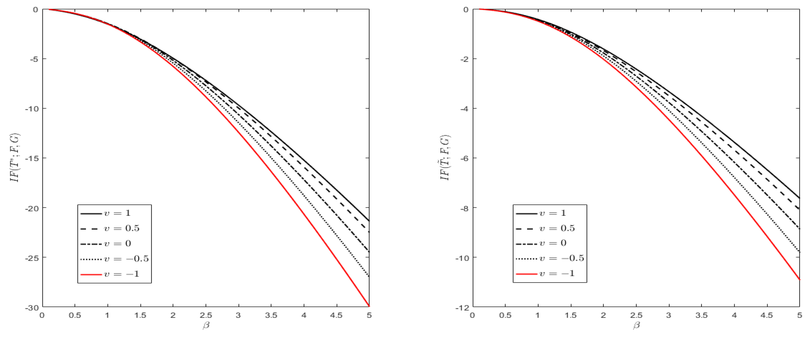
In Figure 3, we take G ( x ) = Γ ( x ; λ , β ) with scale parameter λ = 0.5 and shape parameter β ( 0 , 5 ) , which is a Weibull-type distribution with α = 1 . Its density function g ( x ; λ , β ) is given by
g ( x ; λ , β ) = λ β Γ ( β ) x β 1 exp { λ x } , x > 0 .
We see that, the absolute values of the influence functions of both M-estimations T ˜ n and T n * are increasing in β , and decreasing with v. In other words, with increasing huberization and light-tail contamination, one gets the reduction of sensitivity to deviations from the Weibull model.

4. Simulations

In this section, we carry out a simulation study to illustrate the small sample behavior of M-estimations T ˜ n ( v , ) and T n * ( v , ) compared to the maximum likelihood estimation α ^ m l e = T ˜ n ( 1 , ) and the classical Hill-type estimation α ^ H i l l ( k n ) of the Weibull tail coefficient given by (cf. Girard (2004))
α ^ H i l l ( k n ) = 1 k Σ j = 1 k log ( log n + 1 j ) log ( log n + 1 k + 1 ) 1 k Σ j = 1 k log ( X n j + 1 , n ) log ( X n k , n ) , k = 1 , , n 1 .
To analyze the robustness of the M-estimations, we generate m = 1000 samples of size n = 30 , 50 , 80 and 100 from Weibull distribution F W ( x ; α ) = 1 exp { c 0 x α } , x > 0 contaminated by Gamma distribution Γ ( x ; λ , β ) with contamination level ϵ ( 0 , 1 ) , i.e., the underlying risk follows
F ϵ ( x ) = ( 1 ϵ ) F W ( x ; α ) + ϵ Γ ( x ; λ , β ) .
In the simulations, we take c 0 = 0.5 , 1 , 2 , d 0 = 1 , d 1 = 2 , α = 1 , 2 and λ = β = 0.5 , ϵ = 0.1 , 0.3 . Table 1 lists the average estimations α ¯ , the sample variance s 2 and the ratio of mean squared error (MSE) of MLE, Hill-type estimation to that of T ˜ n and T n * with v = 0 , i.e., ( r ^ , r ˜ , r * ) = ( r ^ 0 , r ˜ 0 , r 0 * ) is given by
r ^ v = M S E ( α ^ H i l l ( k o p t ) ) M S E ( T ˜ n ( v , ) ) , r ˜ v = M S E ( α ^ m l e ) M S E ( T ˜ n ( v , ) ) , r v * = M S E ( α ^ m l e ) M S E ( T n * ( v , ) ) .
Here, we use alternatively k n = k o p t given by (since the traditional optimal choice of k n in Girard (2004) is not available for small samples)
k o p t = arg min k n 1 M S E ( α ^ H i l l ( k n ) ) .
The last column of Table 1 is the relative proportion of k n for which M S E ( α ^ H i l l ( k n ) ) M S E ( T ˜ n ( v , ) ) , denoted by p H i l l , is given by
p H i l l = # { 1 k n n 1 : M S E ( α ^ H i l l ( k n ) ) M S E ( T ˜ n ( v , ) ) } n 1 × 100 % .
The p H i l l describes the percent that the Hill-type estimation outperforms the estimation T ˜ n ( v , ) .
We conclude from Table 1 that
(i)
The bias of the proposed M-estimations is smaller than that of Hill-type estimation and MLE estimation (see columns 2–5 for details).
(ii)
The sample variance s 2 of our estimations is very close to zero. Note by passing that even with the optimal choice of k n = k o p t , the s 2 of Hill-type estimations is still relatively larger than the other (see columns 6–9 for details).
(iii)
Since the ratios of MSE satisfy r ^ r * r ˜ , we see that the best rank estimation is T ˜ n , which coincides with the analysis of the relative efficiency (see columns 10–12 and Figure 2).
(iv)
For n = 30 , 50 , the p H i l l is almost zero indicating that for very small samples T ˜ n ( 0 , ) outperforms Hill-type estimators α ^ H i l l ( k n ) for almost all k n ’s. For n = 80 , p H i l l does not exceed 10 % in most cases which means that there is a set K with at most s = 8 of k n K such that the Hill-type estimators would outperform T ˜ n ( 0 , ) . Similar argument holds for n = 100 . Hence, the M-estimations perform better even for small samples.

5. Empirical Study

The CRIX, a market index (benchmark), is designed by Trimborn and Härdle (2016). It enables each interested party to study the performance of the crypto market as a whole or single crypto market, and therefore attracts increasing attention of risk managers and regulators. We select the daily CRIX index during 31 July 2014–1 January 2018 (available on crix.berlin) and take all n = 713 positive log returns of CRIX multiplied by 15 to obtain a moderate amount of sample of size m around 35–50 greater than 1 for the M-estimation T ˜ n (recall scaled risks keep the same tail decay feature) as the original data sequence X = ( X i , i = 1 , , n ) .
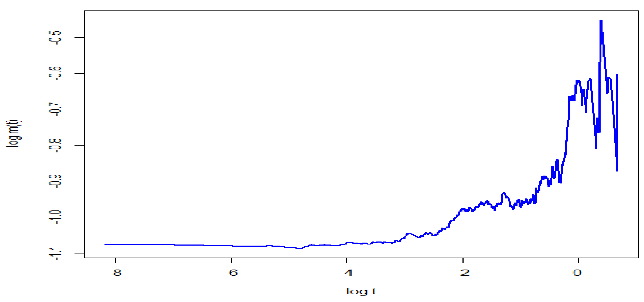
In Figure 4 we employ the empirical mean excess function from extreme value theory to analyze its tail feature (set below I { · } as the indicator function)
m ^ X ( t ) = i = 1 n X i t I { X i > t } i = 1 n I { X i > t } for t large ,
where X i ’s are the scaled daily log returns of CRIX. We see that the log mean excess function behaves linearly for large threshold, indicating the Weibull tail feature of the data-set (cf. Dierckx et al. (2009)).
Therefore, we illustrate the robustness of the proposed M-estimations T ˜ n ( v , ) and T n * ( v , ) with ( d 0 , d 1 ) = ( 0.8848 , 0.9898 ) as the 95 % confidence interval via MLE, and v = 0 using the real data-set X and compare it with the Hill-type estimations α ^ H i l l ( k n ) given by (11). Specifically, we consider the same contamination distribution G ( x ) = Γ ( x ; 0.5 , 0.5 ) and contamination level ϵ = 0.05 i , i = 0 , 1 , , 10 . Besides, the sample fraction k n involved in the Hill-type estimations, is chosen via the bootstrap and maximum likelihood method as follows.
k o p t ( 1 ) = arg min k n 1 | α ^ H i l l ( k n ) α ¯ b H i l l ( k n ) | , k o p t ( 2 ) = arg min k n 1 | α ^ H i l l ( k n ) α ^ m l e | ,
where α ¯ b H i l l ( k n ) is the average value of Hill-type estimations based on m = 100 bootstrap samples, and α ^ m l e is the maximum likelihood estimation of the shape parameter α of Weibull distribution (see (1) for its definition). Due to the unknown Weibull tail coefficient α , we use alternatively the relative deviation of α ^ at contamination level ϵ to ϵ + δ ϵ , denoted by D ( α ^ ) to study the relative robustness. Specifically,
D ( α ^ ) = D e v i a t i o n ( α ^ ) = | α ^ ( ϵ + δ ϵ ) α ^ ( ϵ ) | ,
where α ^ = T ˜ n , T n * , α ^ H i l l ( 1 ) and α ^ H i l l ( 2 ) stand for the M-estimations and Hill-type estimations with optimal choice of k n as in (13), accordingly.
From Table 2, we draw the following conclusions: (i) As expected, the proposed M-estimations are not sensitive to the contaminations, since the relative deviations of M-estimations are almost zero. Conversely, both Hill-type estimations with optimal choices of sample fraction have obvious deviations from no contamination to small contamination ( D ( α ^ H i l l ( 1 ) ) = 0.1277 , D ( α ^ H i l l ( 2 ) ) = 0.2601 for ϵ = 0 ). (ii) The Hill-type estimation α ^ H i l l ( 2 ) , with average value around 0.67, underestimates the α to some extent since the averages of the other three estimations are closer to 0.80.

6. Proofs

Proof of Lemma 1.
Firstly, we show that h * ( t ) , t t 0 is strictly increasing. Indeed, h ( t ) = ( c 0 t 1 ) ln t 1 , t > 0 is twice differentiable and
h ( t ) = c 0 ( ln t + 1 ) 1 t , h ( t ) = c 0 t + 1 t 2 > 0 ,
which imply that h ( t ) , t > 0 is a convex function with a unique minimum h ( t 0 * ) where h ( t 0 * ) = 0 . Therefore, we have t 0 = arg min t 1 h ( t ) exists and the unique solution t 0 = max ( t 0 * , 1 ) and thus h * ( t ) , t [ t 0 , ) is strictly increasing. Noting further for given t 0 1 that t 0 1 / α is strictly decreasing in α , we have h * ( x α ) is strictly increasing in [ x 0 , ) with x 0 = t 0 1 / d 0 t 0 1 / α since α d 0 .
Secondly, note that 1 F ˜ W ( x ; α ) = exp { c 0 ( x α 1 ) } , x 1 . It follows by some elementary calculations that α 1 h ˜ ( x α ) is the score function of F ˜ W ( x ; α ) . Moreover, in view of (15), the minimizer t 0 * of h is decreasing in c 0 . This together with the fact that h ( 1 ) = 1 implies that h ˜ ( y ) = inf { t 1 : h ˜ ( t ) y } , y [ 1 , ) is strictly increasing. ☐
Proof of Theorem 1.
It follows by (5) that ψ ˜ v , u ( y ; α ) is strictly increasing and continuous in α . Hence it suffices to show that
λ ˜ ( α ) : = λ ˜ F W ( α ) = 1 ψ ˜ v , u ( y ; α ) d F ˜ W ( y ; α 0 )
has an isolated root α = α 0 . We have
λ ˜ ( α ) = 1 [ h ˜ ( y α ) ] v u d F ˜ W ( y ; α 0 ) 1 [ h ˜ ( y α ) ] v u d F ˜ W ( y ; α ) = 1 [ h ˜ ( y α ) ] v u d F ˜ W ( y ; α 0 ) μ ˜ , μ ˜ : = v + v u exp { c 0 [ h ˜ ( z ) 1 ] } d z .
Next, it follows by a change of variable t = h ˜ ( y α ) and integration by parts that
1 [ h ˜ ( y α ) ] v u d F ˜ W ( y ; α 0 ) = 1 v v d F ˜ W ( [ h ˜ ( t ) ] 1 / α ; α 0 ) + v u t d F ˜ W ( [ h ˜ ( t ) ] 1 / α ; α 0 ) + u u d F ˜ W ( [ h ˜ ( t ) ] 1 / α ; α 0 ) = v + v u exp { c 0 [ ( h ˜ ( t ) ) α 0 / α 1 ] } d t .
Hence, λ ˜ ( α 0 ) = 0 and
λ ˜ ( α ) = c 0 α 0 α 2 h ˜ ( v ) h ˜ ( u ) s α 0 / α ln s exp { c 0 [ s α 0 / α 1 ] } d h ˜ ( s ) > 0
since h ˜ ( s ) is strictly increasing over [ 1 , ) and
s > h ˜ ( v ) h ˜ ( 1 ) = 1 .
Consequently, the consistency of T ˜ n is obtained.
Next, we show the asymptotic normality of T ˜ n . Set below (recall μ ˜ given in (16))
σ ˜ v , u 2 ( α ) : = 1 ψ ˜ v , u 2 ( y ; α ) d F ˜ W ( y ; α 0 ) = 1 ( [ h ˜ ( y α ) ] v u μ ˜ ) 2 d F ˜ W ( y ; α 0 ) .
Since
σ ˜ v , u 2 ( α ) = 1 v ( v μ ˜ ) 2 d F ˜ W ( [ h ˜ ( t ) ] 1 / α ; α 0 ) + v u ( t μ ˜ ) 2 d F ˜ W ( [ h ˜ ( t ) ] 1 / α ; α 0 ) + u ( u μ ˜ ) 2 d F ˜ W ( [ h ˜ ( t ) ] 1 / α ; α 0 ) = ( v μ ˜ ) 2 + 2 v u ( t μ ˜ ) exp { c 0 [ ( h ˜ ( t ) ) α 0 / α 1 ] } d t = ( v μ ˜ ) 2 + 2 h ˜ ( v ) h ˜ ( u ) ( h ˜ ( s ) μ ˜ ) exp { c 0 [ s α 0 / α 1 ] } d h ˜ ( s )
is finite in a neighbourhood of α 0 and continuous at α = α 0 . It follows thus by Theorem A, p. 251 in Serfling (1980) that T ˜ n is asymptotically normal distributed.
Furthermore, we have by (20)
λ ˜ ( α 0 ) = c 0 α 0 h ˜ ( v ) h ˜ ( u ) s ln s exp { c 0 ( s 1 ) } d h ˜ ( s ) > 0 .
Hence, the asymptotic variance of m ( T ˜ n α 0 ) is given by
σ ˜ v , u , α 0 ; F W 2 = σ ˜ v , u 2 ( α 0 ) [ λ ˜ ( α 0 ) ] 2 .
Please note that m / n p P { X 1 } = exp { c 0 } . We complete the proof of Theorem 1. ☐
Proof of Theorem 2.
Similar arguments of Theorem 1 apply with ψ ˜ , F ˜ W and h ˜ replaced by ψ * , F * and h * , respectively. First we show the consistency of T n * . It follows by (6) that ψ v , u * ( y ; α ) is strictly increasing and continuous in α . Hence it suffices to show that
λ * ( α ) : = λ F W * ( α ) = x 0 ψ v , u * ( y ; α ) d F W * ( y ; α 0 )
has an isolated root α = α 0 . We have
λ * ( α ) = x 0 ψ v , u * ( y ; α ) d F W * ( y ; α 0 ) = x 0 [ h * ( y α ) ] v u d F W * ( y ; α 0 ) x 0 [ h * ( y α ) ] v u d F W * ( y ; α ) = x 0 [ h * ( y α ) ] v u d F W * ( y ; α 0 ) μ * , μ * : = v + v u exp { c 0 ( h * ) ( z ) } d z .
Next, it follows by a change of variable t = h * ( y α ) and integration by parts that
x 0 [ h * ( y α ) ] v u d F W * ( y ; α 0 ) = h * ( x 0 α ) v v d F W ( [ ( h * ) ( t ) ] 1 / α ; α 0 ) + v u t d F W ( [ ( h * ) ( t ) ] 1 / α ; α 0 ) + u u d F W ( [ ( h * ) ( t ) ] 1 / α ; α 0 ) + F W ( x 0 ; α 0 ) [ h * ( x 0 α ) ] | v u = v [ 1 F W ( x 0 ; α 0 ) ] + v u [ 1 F W ( [ ( h * ) ( t ) ] 1 / α ; α 0 ) ] d t + v F W ( x 0 ; α 0 ) = v + v u exp { c 0 ( ( h * ) ( t ) ) α 0 / α } d t ,
where in the second equality we use h * ( x 0 α ) h * ( x 0 d 1 ) = v 0 v . Hence, λ * ( α 0 ) = 0 and
( λ * ) ( α ) = c 0 α 0 α 2 ( h * ) ( v ) ( h * ) ( u ) s α 0 / α ln s exp { c 0 s α 0 / α } d h * ( s ) > 0
since h * ( s ) is strictly increasing over ( x 0 d 0 , ) and
s > ( h * ) ( v ) ( h * ) ( v 0 ) = x 0 d 1 = t 0 d 1 / d 0 1 .
Consequently, the consistency of T n * is obtained.
Next, we show the asymptotic normality of T n * . Set below (recall μ * given by (18))
( σ v , u * ) 2 ( α ) : = x 0 ( ψ v , u * ) 2 ( y ; α ) d F W * ( y ; α 0 ) = x 0 ( [ h * ( y α ) ] v u μ * ) 2 d F W * ( y ; α 0 ) .
Since
( σ v , u * ) 2 ( α ) = h * ( x 0 α ) v ( v μ * ) 2 d F W ( [ ( h * ) ( t ) ] 1 / α ; α 0 ) + v u ( t μ * ) 2 d F W ( [ ( h * ) ( t ) ] 1 / α ; α 0 ) + u ( u μ * ) 2 d F W ( [ ( h * ) ( t ) ] 1 / α ; α 0 ) + F W ( x 0 ; α 0 ) ( v μ * ) 2 = ( v μ * ) 2 + 2 v u ( t μ * ) exp { c 0 ( ( h * ) ( t ) ) α 0 / α } d t = ( v μ * ) 2 + 2 ( h * ) ( v ) ( h * ) ( u ) ( h * ( s ) μ * ) exp { c 0 s α 0 / α } d h * ( s )
is finite in a neighbourhood of α 0 and continuous at α = α 0 , it follows by Theorem A, p. 251 in Serfling (1980) that T n * is asymptotically normal distributed.
Furthermore, we have by (20)
( λ * ) ( α 0 ) = c 0 α 0 ( h * ) ( v ) ( h * ) ( u ) s ln s exp { c 0 s } d h * ( s ) > 0 .
Hence, the asymptotic variance is given by
σ v , u , α 0 ; F 2 = ( σ v , u * ( α 0 ) ) 2 [ ( λ * ) ( α 0 ) ] 2 .
We complete the proof of Theorem 2. ☐
Proof of Theorem 3.
The result follows by analogous arguments as in the proof of Theorem 1. Since ψ ˜ v , u ( x ; α ) is strictly increasing and contionuous in α , the assumptions of Theorem 3 are sufficient for the consistency and asymptotic normality of T ˜ n . Using further Lemma 7.2.1A and Theorem A (see p. 249 and 251 therein) by Serfling (1980), we complete the proof of Theorem 3. ☐
Proof of Theorem 4.
The result follows by analogous arguments as in the proof of Theorem 2. Since ψ v , u * ( x ; α ) is strictly increasing and continuous in α , the assumptions of Theorem 4 are sufficient for the consistency and asymptotic normality of T n * . Using further Lemma 7.2.1A and Theorem A (see p. 249 and 251 therein) by Serfling (1980), we complete the proof of Theorem 4. ☐

Author Contributions

Original Draft Preparation, C.G.; Supervision and Project Administration, C.L.

Funding

This research was funded by the National Natural Science Foundation of China grant (11604375), and Chinese Government Scholarship (201708505031).

Acknowledgments

The authors would like to thank the referees for his\her important suggestions which significantly improve this contribution.

Conflicts of Interest

The authors declare no conflict of interest.

References

  1. Arendarczyk, Marek, and Krzysztof Dȩbicki. 2011. Asymptotics of supremum distribution of a Gaussian process over a Weibullian time. Bernoulli 17: 194–210. [Google Scholar] [CrossRef]
  2. Asimit, Alexandru V., Deyuan Li, and Liang Peng. 2010. Pitfalls in using Weibull tailed distributions. Journal of Statistical Planning and Inference 140: 2018–24. [Google Scholar] [CrossRef]
  3. Basu, Ayanendranath, Ian R. Harris, Nils L. Hjort, and M. C. Jones. 1998. Robust and efficient estimation by minimising a density power divergence. Biometrika 85: 549–59. [Google Scholar] [CrossRef]
  4. Beirlant, Jan, and Jozef L. Teugels. 1992. Modeling large claims in non-life insurance. Insurance: Mathematics and Economics 11: 17–29. [Google Scholar] [CrossRef]
  5. Beran, Jan, and Dieter Schell. 2012. On robust tail index estimation. Computational Statistics & Data Analysis 56: 3430–43. [Google Scholar]
  6. Bingham, Nicholas H., Charles M. Goldie, and Jozef L. Teugels. 1987. Regular variation. In Encyclopedia of Mathematics and Its Applications. Cambridge: Cambridge University Press, vol. 27, ISBN 9780511721434. [Google Scholar]
  7. Dȩbicki, Krzysztof, Julia Farkas, and Enkelejd Hashorva. 2018. Extremes of randomly scaled Gumbel risks. Journal of Mathematical Analysis and Applications 458: 30–42. [Google Scholar] [CrossRef]
  8. Dierckx, Goedele, Jan Beirlant, D. De Waal, and Armelle Guillou. 2009. A new estimation method for Weibull-type tails based on the mean excess function. Journal of Statistical Planning and Inference 139: 1905–20. [Google Scholar] [CrossRef]
  9. Gardes, Laurent, and Stephane Girard. 2008. Estimation of the Weibull tail-coefficient with linear combination of upper order statistics. Journal of Statistical Planning and Inference 138: 1416–27. [Google Scholar] [CrossRef]
  10. Girard, Stephane. 2004. A Hill type estimator of the Weibull tail-coefficient. Communications in Statistics-Theory and Methods 33: 205–34. [Google Scholar] [CrossRef]
  11. Goegebeur, Yuri, Jan Beirlant, and Tertius De Wet. 2010. Generalized kernel estimators for the Weibull-tail coefficient. Communications in Statistics-Theory and Methods 39: 3695–716. [Google Scholar] [CrossRef]
  12. Goegebeur, Yuri, Armelle Guillou, and Theo Rietsch. 2015. Robust conditional Weibull-type estimation. Annals of the Institute of Statistical Mathematics 67: 479–514. [Google Scholar] [CrossRef]
  13. Hashorva, Enkelejd, and Zhichao Weng. 2014. Tail asymptotic of Weibull-type risks. Statistics 48: 1155–65. [Google Scholar] [CrossRef]
  14. Huber, Peter J. 1964. Robust estimation of a location parameter. The Annals of Mathematical Statistics 35: 73–101. [Google Scholar] [CrossRef]
  15. Kundu, Debasis, Debanjsn Mitra, and Ayon Ganguly. 2017. Analysis of left-truncated and right-censored competing risks data. Computational Statistics & Data Analysis 108: 12–26. [Google Scholar]
  16. Liu, Yan, and Qihe Tang. 2010. The subexponential product convolution of two Weibull-type distributions. Journal of the Australian Mathematical Society 89: 277–88. [Google Scholar] [CrossRef]
  17. Serfling, Robert J. 1980. Approximation Theorems of Mathematical Statistics. New York: John Wiley & Sons, ISBN 9780471024033. [Google Scholar]
  18. Trimborn, Simon, and Wolfgang K. Härdle. 2016. CRIX an Index for Blockchain Based Currencies. SFB 649 Discussion Paper 2016-021. Berlin: Economic Risk. [Google Scholar]
  19. Vandewalle, Bjorn, Jan Beirlant, and Mia Hubert. 2004. A robust estimator of the tail index based on an exponential regression model. In Theory and Applications of Recent Robust Methods. Berlin and Heidelberg: Springer, pp. 367–76. [Google Scholar]
  20. Vandewalle, Bjorn, Jan Beirlant, Andreas Christmann, and Mia Hubert. 2007. A robust estimator for the tail index of Pareto-type distributions. Computational Statistics & Data Analysis 51: 6252–68. [Google Scholar]
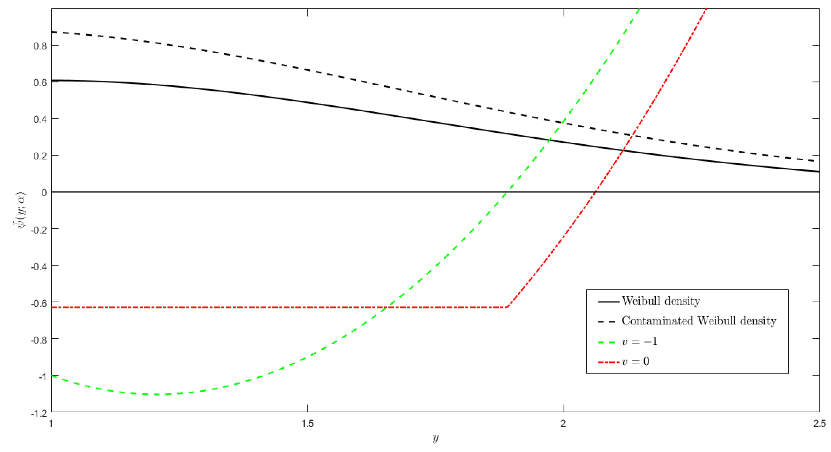
Figure 1. Psi-functions ψ ˜ for the huberized M-estimators T ˜ n ( v , ) . Here the truncated densify functions are generated from the Weibull F W ( x ; α ) and contaminated Weibull F ϵ ( x ) = ( 1 ϵ ) F W ( x ; α ) + ϵ Γ ( x ; λ , β ) with α = 2 , c 0 = 0.5 , ϵ = 0.3 , λ = 1 , β = 1 .
Risks 06 00119 g001
Figure 2. Relative asymptotic efficiency (AEFF) of T ˜ n ( v , ) and T n * ( v , ) compared to the MLE T ˜ n ( 1 , ) . Here F W ( x ; α 0 ) is given by (1) with c 0 = 1 , α 0 = 1 .
Risks 06 00119 g002
Figure 3. Influence functions I F ( T ; F , G ) for T = T ˜ n ( v , ) (left) and T n * ( v , ) (right). Here G ( x ) = Γ ( x ; λ , β ) , λ = 0.5 , β ( 0 , 5 ) , v = ± 1 , ± 0.5 , 0 and F ( x ) = F W ( x ; α 0 ) is given by (1) with c 0 = 1 , α 0 = 1 .
Risks 06 00119 g003
Figure 4. Graph of log mean excess function of scaled log returns of daily CRIX during 31 July 2014–1 January 2018.
Risks 06 00119 g004
Table 1. Comparisons of T ˜ n , T n * with α ^ m l e , α ^ H i l l ( k n ) . Here we take m = 1000 samples of size n = 30 , 50, 80, 100 from F ϵ ( x ) = ( 1 ϵ ) F W ( x ; α ) + ϵ Γ ( x ; 0.5 , 0.5 ) .
( ϵ , c 0 , α ) n α ¯ mle α ¯ Hill T ˜ n T n * s mle 2 s Hill 2 s T ˜ 2 s T * 2 r ^ r ˜ r* p Hill
(0.3, 1, 1)300.92170.82551.00061.00050.00720.04510.00180.001568.68118.77748.36780.00
500.86090.84351.00221.00610.00680.02890.00140.001523.128814.340713.43440.00
800.82740.83261.00831.00750.00410.01760.00130.00169.748519.597219.23930.00
1000.81610.83681.01471.01190.00300.01480.00180.00156.260720.814320.08420.00
(0.1, 1, 1)300.98850.93430.99420.99400.00070.04690.00070.00065.72871.22831.05610.00
500.98340.92520.99490.99520.00090.02690.00070.00063.64071.81941.80000.00
800.97760.94070.99620.99530.00090.01890.00050.00061.00062.58492.38290.00
1000.97350.93020.99640.99610.00100.01300.00050.00050.71383.25492.96230.15
(0.3, 1, 2)301.23821.60391.99601.99190.06870.24080.00560.005074.7362147.2932126.86530.00
501.13471.64432.00151.99630.02680.15760.00450.004222.7834158.1670165.11270.00
801.08511.68532.00502.00390.01270.12190.00390.00387.8035197.7217180.37460.00
1001.07311.67092.00812.00730.00850.08830.00420.00385.1102223.2889186.39960.00
(0.1, 1, 2)301.92451.83991.99031.98590.01690.20250.00260.00244.88339.35668.41480.00
501.84591.85061.99001.98880.02390.12230.00220.00213.123321.457618.46490.00
801.76541.83921.98731.98950.02280.07540.00170.00173.075839.654735.45840.00
1001.72491.86811.98981.99060.01900.06600.00180.00181.914243.165645.15570.00
(0.3, 2, 1)300.94660.86400.99740.99870.00470.04290.00160.002182.55584.60143.53350.00
500.90610.88810.99550.99650.00510.02980.00150.001322.783412.701310.12860.00
800.87290.88480.99440.99550.00360.01720.00120.00103.299016.110916.02860.00
1000.85620.89380.99700.99780.00290.01520.00110.00111.714619.840718.13230.00
(0.1, 2, 1)300.98800.92230.99530.99560.00050.27730.04830.00115.19040.88480.72320.00
500.98520.95570.99410.99520.00070.14380.02610.00063.46811.23801.10710.00
800.98080.94520.99400.99420.00080.17750.01650.00050.95242.03531.65220.10
1000.97620.95600.99270.99390.00090.04440.01480.00060.85892.37732.24940.12
(0.3, 2, 2)301.30191.60181.98551.98530.05830.24340.00300.002685.6893153.3920159.48660.00
501.20121.65891.98501.98500.02280.12090.00240.002114.7957260.7202270.02560.00
801.15701.67011.98441.98380.00991.10060.00180.00172.5650348.1278345.65870.00
1001.14841.67711.98321.98300.00690.07120.00170.00171.4158386.5744370.88520.00
(0.1, 2, 2)301.92381.80541.98851.98700.01610.17630.00270.00324.31615.84396.34420.00
501.85191.86371.98861.98500.02120.12010.00310.00233.938817.654816.92910.00
801.76461.85651.98691.98490.02000.06960.00170.00191.258837.791236.67440.00
1001.74021.88391.98491.98430.01810.07560.00170.00170.979147.860144.64770.05
(0.3, 0.5, 1)300.93200.79891.00561.00650.00480.05650.00120.00147.24977.72316.79770.00
500.89120.82501.01161.00960.00510.04680.00120.00138.846512.230910.27650.00
800.85650.81301.01851.01880.00340.02610.00130.00122.835515.429414.89020.00
1000.84630.83681.02181.02320.00240.02520.00110.00121.317517.004516.52850.00
(0.1, 0.5, 1)300.98740.88480.99680.99430.00050.04280.00060.00065.37881.21571.02360.00
500.98530.91360.99720.99520.00050.02950.00050.00053.84571.51111.49740.00
800.97990.91930.99770.99750.00060.01810.00040.00051.94362.35281.97080.00
1000.97830.91650.99910.99890.00060.01430.00050.00040.92412.28652.18400.10
(0.3, 0.5, 2)301.32771.59642.00651.81440.07130.25040.00520.000461.5168111.591815.10110.00
501.21411.62432.01851.80830.03730.16070.00490.000331.3754129.648917.78500.00
801.16181.65962.03571.80420.01470.10470.00460.000213.2211128.053018.89150.00
1001.14861.67072.03861.80350.01250.09740.00470.00024.5564118.170819.16170.00
(0.1, 0.5, 2)301.94431.85891.99001.80400.00930.20910.00200.00058.53296.75370.34540.00
501.89361.87451.99351.79630.13160.65200.00200.00034.906012.63720.58320.00
801.83291.82711.99581.79370.07200.64080.00180.00021.352422.13260.92320.00
1001.81251.85382.00241.79300.06702.81630.00170.00020.956126.71881.03630.08
Table 2. Estimations of Weibull tail coefficient and its relative deviations via contamination level ϵ = 0.05 i , i = 0 , , 10 . Data is the positive and scaled log returns of daily CRIX during 31 July 2014–1 January 2018.
ϵ T ˜ n T n * α ^ Hill ( 1 ) α ^ Hill ( 2 ) D ( T ˜ n ) D ( T n * ) D ( α ^ Hill ( 1 ) ) D ( α ^ Hill ( 2 ) )
0.000.77110.79320.92020.93590.00720.00550.12770.2601
0.050.77830.79870.79250.67580.00560.00600.00840.0246
0.100.78390.80470.80090.65120.00020.00050.00380.0028
0.150.78410.80520.80470.64840.00260.01440.02580.0172
0.200.78670.81960.83050.63120.00930.01170.05600.0094
0.250.79600.83130.77450.64060.00460.01860.01680.0075
0.300.80060.84990.75770.63310.00460.00920.00380.0089
0.350.79600.84070.75390.64200.01200.00840.01680.0049
0.400.80800.84910.77070.63710.00080.00960.03700.0029
0.450.80720.85870.73370.64000.00690.00520.02080.0096
0.500.80030.86390.75450.6304----