Abstract
In this paper, we propose a clustering procedure of financial time series according to the coefficient of weak lower-tail maximal dependence (WLTMD). Due to the potential asymmetry of the matrix of WLTMD coefficients, the clustering procedure is based on a generalized weighted cuts method instead of the dissimilarity-based methods. The performance of the new clustering procedure is evaluated by simulation studies. Finally, we illustrate that the optimal mean-variance portfolio constructed based on the resulting clusters manages to reduce the risk of simultaneous large losses effectively.
1. Introduction
It is of great interest in identifying the risk of simultaneous large losses in portfolio selection and financial risk management. If this type of risk is identified properly, candidate assets could be grouped such that asset prices or returns from different groups are unlikely to drop simultaneously. An investment strategy is called portfolio diversification if the portfolio is constructed by selecting one asset from each group. As we could see, the performance of portfolio diversification depends on how the assets are grouped.
In general, the observed prices or returns of assets are essentially time series. To group assets properly, time series clustering techniques are usually involved. Early works on time series clustering include interdependence measure between asset returns such as the (Pearson or Spearman type) cross-correlation coefficients (cf. Kaufman and Rousseeuw 1990). In particular, Mantegna (1999) and Bonanno et al. (2004) quantified the degree of interdependence between the synchronous time evolution of a pair of stock prices and used it in financial time series clustering. Moreover, as another extension of dependence-based method, Baragona (2001) and Brockwell and Davis (2002) developed a new measure of interdependence from the residuals obtained by fitting the data to acceptable time series. In addition, inspired by the dynamic conditional correlation (DCC) model developed by Engle and Sheppard (2001) and Engle (2002), Billio et al. (2006) and Billio and Caporin (2009) proposed the Flexible Dynamic Conditional Correlation (FDCC) multivariate GARCH model and provided an estimate of the dynamics of correlation coefficients within groups of financial assets for asset allocations.
However, cross-correlation coefficients do not always guarantee a sufficient degree of portfolio diversification because these coefficients cannot always capture the possible extreme co-movements of asset returns in lower tails. Extreme co-movement of asset returns in lower tails plays an important role in studying contagion of financial crisis. Bae et al. (2003) provided evidence of the existence of extreme co-movements in terms of coexceedances when studying the phenomenon of contagion. More formally, the contagion of financial crisis could be defined directly as a significant increase of extreme co-movements if financial crisis occurs in one of the markets (cf. Pericoli and Sbracia 2003, Definition 4). Hence, if a portfolio diversification arrangement fails to diversify the risk of extreme co-movement in the lower tail, it might be vulnerable to the contagion of financial crisis occurring in other markets.
Even when there is no contagion, extreme co-movements of asset returns may also exist due to the similarity of fundamentals from the traditional point of view, investor trading patterns(Barberis et al. 2005), or incomplete information (Veldkamp 2006). To diversify the risk of extreme co-movement in lower tail, De Luca and Zuccolotto (2011) proposed a dissimilarity measure based on tail dependence coefficients (TDC) instead of cross-correlation coefficients to obtain homogeneous groups of time series with an association between extreme low values. Inspired by this work, Durante et al. (2014) developed a time series clustering procedure with a conditional version of Spearman’s correlation coefficient for extremely low values introduced by Durante et al. (2014), and a non-parametric estimator of tail dependence provided in Durante et al. (2015). De Luca and Zuccolotto (2015) further proposed a dynamic clustering procedure so that the coefficient employed to measure the lower tail dependence can be time-varying on the basis of historical market volatility.
In this paper, we propose to cluster time series via the coefficients of maximum tail dependence introduced by Furman et al. (2015). The coefficients of maximal tail dependence are direct extensions of TDCs including the tail dependence coefficient , the weak tail dependence coefficient and the tail order . The major difference is that the coefficients of maximal tail dependence are calculated with convergence paths that are possibly other than the diagonal path. As a result, the matrix of coefficients of maximal tail dependence may not be symmetric and thus cannot be used as a similarity (or dissimilarity) matrix in clustering procedures. Instead, such a matrix may be seen as a type of affinity matrix representing directed relations between assets.
The paper is organized as follows. Section 2 is a brief introduction of the coefficients of maximal tail dependence. The proposed clustering procedure of time series is formally described in Section 3. The performance of the proposed procedure is evaluated in Section 4. An application to real exchange rates of G20 countries is presented and analyzed in Section 5. Section 6 concludes.
2. The Coefficients of Maximal Tail Dependence
Several coefficients have been introduced by researchers to measure the extreme co-movements in recent years. For example, one of the most important measures is the lower (upper) tail dependence, which is formally defined by
where random variables X and Y represent the potentially dependent risks. Since by Sklar’s Theorem (cf. Nelsen 2006) there is a uniquely determined copula function such that
the lower (upper) tail dependence could be defined as the limiting point of a functional of the copula function, namely,
where is the survival copula with respect to C. Apart from the lower (upper) tail dependence, similar measures include the weak lower (upper) tail dependence
(cf. Coles et al. 1999) and lower (upper) tail order () defined via:
where and are slowly varying functions of u at 0 (cf. Hua and Joe 2011).
The aforementioned measures of tail dependence are all limiting values of functionals of C as the arguments shrink to along the diagonal line of the square . However, as pointed out by Furman et al. (2015), these measures may sometimes underestimate the extent of extreme co-movements for dependent risks, and, for this reason, the authors proposed improved versions of these coefficients of tail dependence, named as the coefficients of the maximal tail dependence, which are more sensitive to extreme co-movements. Accordingly, a clustering procedure based on such coefficients may provide better clustering results than those based on other coefficients of tail dependence such as those proposed by De Luca and Zuccolotto (2011) and Durante et al. (2014), and the portfolios constructed based on such clustering results may also outperform.
The coefficients of the maximum tail dependence are limiting values of the usual versions of the corresponding functionals of C (or ) converging to the lower-left (or upper-right) vertex along paths of maximal tail dependence. To formally define the paths of maximal tail dependence, consider a function satisfying the following admissible conditions (see Furman et al. 2015, Definition 2.1):
- for every ; and
- both and converge to 0 when .
The collection of such kind of functions is called the admissible set, denoted as . Then, a path shrinking to the lower-left (or upper-right) vertex is called admissible whenever belongs to . Specifically, the diagonal path used to define the usual coefficients of tail dependence is admissible as the function , is admissible. According to (Furman et al. 2015, Definition 2.2), the paths of maximal tail dependence is denoted as where
To simplify the notations, we denote if the optimal value exists. Then, the lower tail maximal dependence (LTMD) is defined via:
the weak lower tail maximal dependence (WLTMD) is defined via:
and the order of lower tail maximal dependence is defined via:
where is a slowly varying function of u at 0. In particular, for , we have the following result similar to that of the usual tail order (cf. Hua and Joe 2011):
Proposition 1.
For any bivariate copula function C, if exists, then the corresponding index of maximal tail dependence .
The proof is given in Appendix A. As a result, may also not be a desirable affinity measure for common clustering procedures such as k means clustering or hierarchical clustering. However, is a desirable weight for graphs. The larger of two assets is, the stronger the extreme co-movement between these assets is, and hence a bigger weight is posed by .
We refer to Furman et al. (2015) for examples of expressions for and with closed forms in the case of parametric families of distributions. Notably, Furman et al. (2016) proved that, in the Gaussian case, the classical and maximal tail dependence coefficients coincide. In the present paper, however, to speed up practical calculations, we resort to non-parametric approach in the following sections. In particular, we find a clustering procedure based on to be very attractive.
3. Clustering Procedure
Typically, clustering based on dissimilarity matrices such as given by De Luca and Zuccolotto (2011, sct. 3) could be achieved through the hierarchical clustering method directly. However, to cluster using the affinity matrix constructed with , we could not use the hierarchical clustering method because the affinity matrix may not be symmetric. Hence, we have to consider graph based clustering procedures.
Suppose we have n assets in total available for a portfolio construction. Then, the affinity matrix is given by
(cf. Furman et al. 2015, sct. 5). Theoretically, should be a symmetric matrix which could be seen as an affinity matrix consisting of edge weights for an undirected graph and thus could be used for clustering with the hierarchical clustering method. This is because is unique as long as it exists and thus . However, for those asymmetric copulas such as the unexchangeable Marshall–Olkin copulas
the estimated parameters may differ due to that for two series of observations there are actually two different copulas to be chosen for the parameter estimation procedure: and . In other words, for two arbitrary series of observations, it is impossible to determine which group should be regarded as “u” and the other group as “v” in practice, even though we are sure that these observations are generated from an unexchangeable Marshall–Olkin copula.
For simplicity, when constructing the affinity matrix , we keep only one of the two possible copulas whenever we have to estimate the parameters of the copula from pairwise observations. The advantage of this idea is that, taking for instance, the lower triangle part of is calculated by assuming the pairwise observations are generated from and then estimating the parameters a and b while the upper triangle part of is actually calculated by assuming the same pairwise observations are generated from and then estimating the parameters a and b. In other words, the resulting affinity matrix contains information of estimated parameters from both and in fact.
Since such an affinity matrix may not necessarily be symmetric, the hierarchical clustering method fails to work. In this case, the resulting affinity matrix could be considered as a matrix of weighted edges in a directed graph instead of an undirected graph. The clustering task could be achieved with the Weighted Normalized Cuts (WNACut for short) introduced by Meilă and Pentney (2007), which is initially developed to analyze directed graphs related to the link data.
To understand the WNACut method, let be an arbitrary partition of the set of all assets. Then, the cut of to represents the total influence of Cluster on Cluster , namely,
Hence, the total weighted cut of all clusters is defined via:
where for . Then, our target cluster is such that
This optimization problem could be solved through a spectral clustering algorithm named “Best WCut”. Similar to the clustering procedure proposed by De Luca and Zuccolotto (2011), this algorithm is also a two-stage clustering procedure, in which the non-metric multidimensional scaling (MDS) in the first stage is substituted by a process that transforms the asymmetric affinity matrix consisting of the WLTMDs into k orthonormal columns, where k is the predetermined number of clusters. The details are given in Algorithm A1. In Meilă and Pentney (2007), the WNACut method is shown to consistently outperform all other clustering methods chosen to be tested with synthetic data in their experiments. For this reason, we adopt this method to finish the clustering task in our proposed procedure.
4. A Simulation Study of Synthetic Data
As mentioned, our proposed clustering procedure is a two-stage procedure, as shown in Algorithm A1. However, there is no information related to the choice of clustering method for the second stage in this particular situation revealed. Hence, a simulation study is designed in this section to compare the performance of the second stage clustering method in WNACut with that of a list of commonly used clustering methods, including the classical k-means method and hierarchical clustering procedure with Ward’s minimum variance method (considering both Ward’s criterion and Ward’s criterion squared, the results are denoted as Ward.D2 and Ward.D, respectively), single linkage method, complete linkage method, average linkage method, McQuitty’s linkage method, median linkage method, and centroid linkage method. The performances are measured in two metrics: the misclassification error (ME) described in Verma and Meilă (2003) and variation in information (VI) introduced in Meilă (2003). Both criteria tend to be smaller if the resulting clusters are more similar to the K known clusters.
To begin with, we assume there are K different known clusters whose numbers of elements are , respectively. The dependence structure employed to generate the realizations in each cluster is a particular case of the asymmetric multivariate copula given by Liebscher (2008, eq. 3); namely, for cluster k, we have
where and . Then, the joint CDF of the distribution used to generate the realizations is given by
Notice that, with the above model settings, the pairwise marginal copulas could be written as either
or
which includes both the pairwise independent copula as the particular case and the pairwise standard Clayton copula as the particular case . Then, as discussed in Section 3, we only keep (3) for further analysis. When the realizations are generated, the affinity matrix consisting of pairwise WLTMDs could be calculated by first estimating and with the maximal likelihood method based on (3) and then calculating the WLTMDs using
(cf. Furman et al. 2015, eq. 6.2). Therefore, with all pairwise obtained, the affinity matrix could be calculated through Equation (1). Then, given the predetermined number of clusters k, the first stage of the BestWCut will transform the affinity matrix into k orthonormal columns.
The total number of iterations for our simulation study is 500, which is the same as De Luca and Zuccolotto (2011). Other values of the parameters for the simulation study are given below:
- The number of known clusters .
- The number of objects in each cluster are independently sampled from at random for each iteration.
- .
- , which result in theoretical , respectively, if the two series of realizations are neither independent nor dependent with a classical Clayton copula.
- The distances used in hierarchical clustering methods are all Euclidean distance in .
The results of MEs and VIs are given in Table 1 and Table 2, respectively, in which we can see that, with Ward’s criterion squared, the Ward’s minimum variance method is consistently competitive or even outperforms other methods. Moreover, the distributional properties of the simulated ME’s are shown in Figure 1, Figure 2 and Figure 3 for , , and , respectively, and the distributional properties of the simulated VIs are shown in Figure 4, Figure 5 and Figure 6 for , , and , respectively. All these figures indicate that the Ward’s minimum variance method might be the best choice for the second stage of the proposed clustering procedure.

Table 1.
Means and variances of simulated MEs using various clustering methods in the second stage of WNACut for , and , respectively.
Table 2.
Means and variances of simulated VIs using various clustering methods in the second stage of WNACut for , and , respectively.
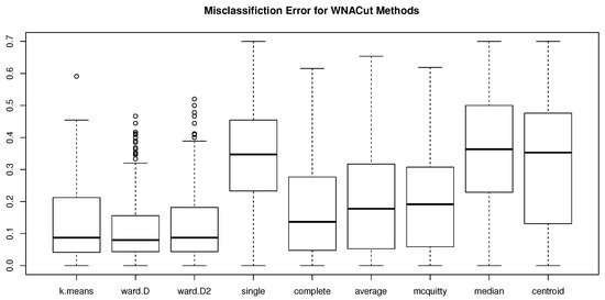
Figure 1.
Box plots of simulated MEs using various clustering methods in the second stage of WNACut for .
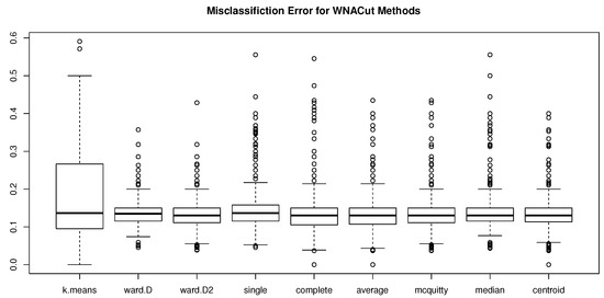
Figure 2.
Box plots of simulated MEs using various clustering methods in the second stage of WNACut for .
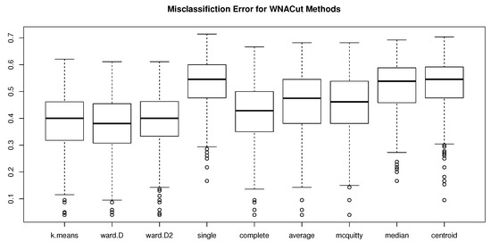
Figure 3.
Box plots of simulated MEs using various clustering methods in the second stage of WNACut for .
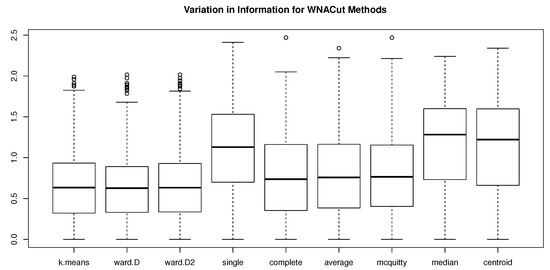
Figure 4.
Box plots of simulated VIs using various clustering methods in the second stage of WNACut for .
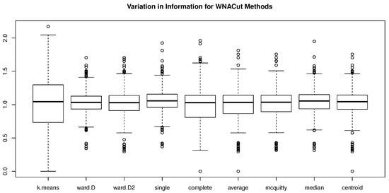
Figure 5.
Box plots of simulated MEs for all hierarchical clustering methods when .
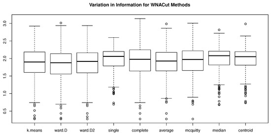
Figure 6.
Box plots of simulated VIs using various clustering methods in the second stage of WNACut for .
The results shown in Table 1 and Table 2 also indicate the sensitivity of the ME/VI to . Taking the Ward’s minimum variance method as an example, when increases or decreases by () (i.e., increases from 8 to 64 or decreases from 8 to 1, correspondingly) the average ME increases by or decreases by , correspondingly, while the average VI increases by or decreases by , correspondingly. Thus, our proposed clustering procedure seems to perform better as the true WLTMD gets closer to 1, and as the true WLTMD moves towards 2, the performance of our proposed clustering procedure worsens rapidly.
5. Application to Real Data
In this section, we apply the proposed procedure on the log-returns of foreign exchange rates with respect to US dollars from Group of 20 (known as G20). Since US dollar is used as the underlying currency, there are 19 time series of exchange rates in total. The exchange rates of France, Germany and Italy are excluded from our analysis due to their perfect linear correlation with euros, which results in 16 time series of exchange rates available for our clustering analysis1. The data were collected weekly from 5 September 2012 to 17 August 2016, covering 207 × 16 active observations during these four years, which can be downloaded from “PACIFIC Exchange Rate Service”, 2016, by Werner Antweiler, University of British Columbia. The descriptive statistics and histograms of observations for the 16 currencies are given in Table 3 and Figure 7.
Table 3.
Descriptive statistics of (log)returns of 16 selected currencies.
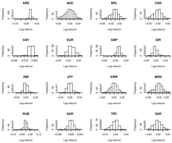
Figure 7.
Histograms for the 16 selected currencies.
5.1. Preliminary Analysis
For each series of the exchange rates, the log-returns are obtained by taking logarithm of the fraction between two consecutive weekly exchange rates, part of which are shown in Figure 8. To eliminate the potential autocorrelation and heteroskedasticity of the log-returns, a univariate generalized error distribution (GED) ARMA-GARCH model is applied to each time series of log-returns and the fitted standardized residuals are extracted for the purpose of clustering.
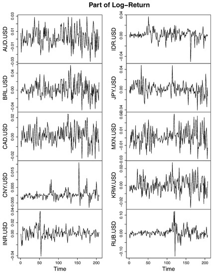
Figure 8.
Log return of exchange rates for some of the G20 members.
A preliminary test of correlation indicates that the standardized residuals of Argentine Pesos seem to be uncorrelated to those of all the other currencies. The details of the correlation tests are shown in Table 4, from which we could see that all p-values are greater than . Thus, we suspect that all WLTMDs between the residuals of ARS and any other currency are approximately 0. To this end, let where X represents some currency and is the random variable having the same distribution as the standard residuals obtained by fitting the log-returns of currency X with GED ARMA-GARCH model. Then, by Coles et al. (1999, eq. 4.2), we have
as where and is the weak lower-tail dependence between the standard residuals of the log-returns of ARS and currency X. Hence, our concern about whether is equivalent to test
Table 4.
The p-values of correlation tests between the standardized residuals of ARS and those of the other 15 currencies based on Pearson’s product moment correlation coefficient, Kendall’s and Spearman’s , respectively. The last column contains the p-values of the test of using the OLS test statistic.
The test statistic, which is asymptotically standard normal, could be obtained using the improved OLS method given in Gabaix and Ibragimov (2011). When 50 pairs of observations are used, the resulting p-values are all greater than , as shown in Table 4. Thus, could not be rejected, which leads to and hence for all currencies other than ARS. Notice that by definition WLTMD should always be smaller than or equal to the corresponding weak lower-tail dependence, therefore the WLTMDs between the residuals of ARS and those of any other currency are approximately 0, which allows us to evaluate ARS as an isolated point that will not be taken into account in further analysis.
In fact, ARS is not the only currency that should be excluded from further clustering procedure. When testing the correlation between standardized residuals of the fitted GED ARMA-GARCH model for log-returns, we discover that the residuals of SAR have negative correlation with majority of the residuals of the other currencies (see the columns entitled “Sign of estimated coefficients” in Table 5). Furthermore, we can see in Table 5 that only AUD, CNY, GBP and JPY are currencies whose standard residuals may not be negatively correlated with SAR. Unfortunately, none of the corresponding p-values show significant correlation between the standardized residuals of these currencies and SAR. Therefore, it is reasonable to suspect the WLTMDs between the residuals of SAR and any other currency are approximately 0. As expected, the last column in Table 5 verifies this result using the OLS test statistics with only 30 pairs of observations. Therefore, we do not include SAR in our next step of clustering procedure either.
Table 5.
The sign of Estimated Correlation Coefficients and p-values of correlation tests between the standardized residuals of SAR and those of the other 14 currencies based on Pearson’s product moment correlation coefficient, Kendall’s and Spearman’s , respectively. The last column is the p-values of the test of using the OLS test statistic.
Since there are no more currencies that could be evaluated as isolated points based on correlation tests or OLS test statistics, we retain all of the rest 14 exchange rates in our further clustering analysis.
5.2. Clustering the Exchange Rates Using WLTMD
For each pair of the residuals fitted from the log-return series, a bivariate Clayton copula function (see Liebscher 2008, for instance) is adopted with the form of Equation (3) on the estimated empirical distribution functions (pseudo observations), where and are unknown parameters to be specified. Notice that the Clayton-type copula defined in Equation (3) relaxes the restriction in the classical Clayton copula and hence is not necessarily symmetric. With this Clayton-type copula, the tail order of maximal dependence is proved to have the following analytic form:
(cf. Furman et al. 2015, eq. 6.2). The parameters can be estimated by the maximum likelihood method, and hence the estimate of the lower tail of the maximal dependence is given by . To measure the goodness-of-fit of the assumed copula, we employ a test based on the Rosenblatt transformation (see Breymann et al. 2003) between two dependent random variables and , given by
where denotes the standard normal c.d.f. and the conditional copula. Then, the random variable should have a distribution if C is the true copula, which can be tested by a Kolmogorov–Smirnov test between S as a function of pseudo observations and for each pair of the standardized residuals for different currencies. The test statistics are given in Table A1 in Appendix C. Notice that in our situation, thus the critical value for the Kolmogorov–Smirnov test is equal to , indicating none of the fitted copulas should be rejected as the true copulas.
Using the fitted parameters and , we obtain the fitted tail order of maximal dependence as well as the fitted WLTMD . Then, we apply the WNACut algorithm for the first stage of the clustering procedure and Ward1 method for the second stage on the affinity matrix constructed by the ( 196) s for , respectively. The total weights for WNACut is k, and the percentages of weights cut of the total weights against k are shown in Figure 9, which indicates that a relatively stable clustering result is obtained when the number of clusters .
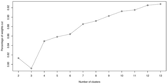
Figure 9.
Percentage of weights cut against the number of clusters.
To get a closer look at the clustering result, first we consider the case whose cluster dendrogram is given by Figure 10.
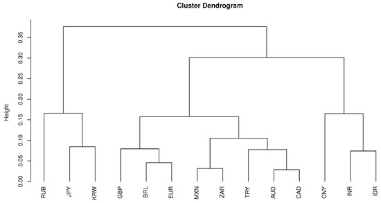
Figure 10.
The dendrogram of the clustering procedure based on WNACut methods with affinity matrix as WLTMDs for .
The resulting clusters are listed in Table 6 which provides a regional segmentation of the world: Northeast Asia, the East/Southeast Asia and the rest of the world. Obviously, such a cluster result has the lowest percentage of weighted cuts and seems to perform well for currencies of countries in the Northeast Asia, East Asia and Southeast Asia. However, it fails to distinguish the currencies of the rest of the world. For the purpose of comparison, in Table 6, we also provide the clustering results given by the method of De Luca and Zuccolotto (2011) for .
Table 6.
Members for each of the clusters when .
Next, we compare the clustering result for to . When , the clustering dendrogram is given by Figure 11.
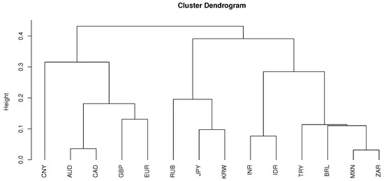
Figure 11.
The dendrogram of the clustering procedure based on WNACut methods with affinity matrix as WLTMDs for .
The resulting clusters are listed in Table 7 which preserves the regional characteristics for currencies of countries in East/Northeast Asia while the partition of the rest of the world in Table A2 is provided by the IMF. For the purpose of comparison, in Table 7, we also provide a clustering result given by the method of De Luca and Zuccolotto (2011) for . Here are some remarks on the clustering outcomes obtained by our clustering procedure.
Table 7.
Members for each of the clusters when .
- All economies in the first group have strong economic connections with the US (under certain type of free trade agreements). Besides, the nominal per capita GDPs of these economies are all above (see Table A2 in Appendix D). Thus, it is reasonable to include currencies of these economies in one group.
- The second group of economies have neither strong economic connection to the US nor high nominal per capita GDPs (less than ). Moreover, all of them are identified as emerging economies by IMF (see Table A2 in Appendix D).
- China is the only member of the third group. Although there is no free trade agreements between US and China, it is well-acknowledged that China has a strong economic connection with the US. In addition, China has a very high nominal GDP (the third highest among all 20 economies) but very low nominal GDP per capita (less than ). As a result, it is reasonable to not include China in any other group.
- It is reasonable to include the rest three economies in one group from the geographical perspective.
In conclusion, the clustering result for seems to more reasonable compared to that of . Besides, the clustering result for could not be obtained through further partition based on the clustering result for because it requires a combination of {Brazil, Mexico, South Africa, Turkey} and {India, Indonesia} as a new cluster. Therefore, the clustering result for seems not to be sufficiently stable from our perspective.
5.3. An Example of Portfolio Management with the Clustering
As stressed in Section 1, one important application of time series clustering is risk management. Since the WLTMD represents the extreme co-movement downwards, the resulting clusters obtained through our proposed procedure represent groups of assets whose returns move in the same direction when both returns are extremely low. Hence, we should avoid including two assets from the same cluster in our portfolio. For instance, if we would like to construct a portfolio with four of the 14 aforementioned currencies, we may consider the following steps:
- Perform our proposed clustering procedure for . The clustering result is given in Table 7.
- From the clustering result in Table 7, one has () 72 choices if he/she tries to avoid selecting two assets from the same cluster in his/her portfolio. All 72 resulting portfolios are listed in Table A3 in Appendix E.
- Construct portfolio using Markowitz’s procedure (minimum variance criteria), namely, computing the sample covariance matrix of the log-returns for any combination of currencies in Table A3 and solvingsubject to and for , where . The resulting weights corresponding to the 72 choices of currencies are also given in Table A3 in Appendix E.
The paths of the returns for all 72 combinations are shown in Figure 12. Notice that there are () 1001 different combinations of four currencies without considering the clustering result (the resulting weights as well as the mean and accumulative returns corresponding to these 1001 portfolios are listed in Table S1 in the Supplementary Materials). We also construct portfolios using Equation (5) for all of the 1001 combinations of currencies and plot the corresponding paths of returns in Figure 12. In contrast, in Figure 12, we also provide the paths of aggregated returns of all portfolios constructed by the method of De Luca and Zuccolotto (2011).
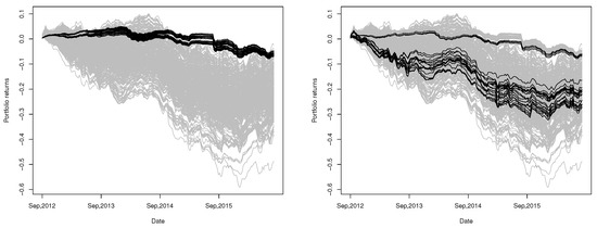
Figure 12.
Returns (black lines) of the selected minimum variance portfolios based on our clustering procedure (left, 72 portfolios in total) and the procedure proposed by (De Luca and Zuccolotto (2011)) (right, 32 portfolios in total). Each portfolio consists of four currencies, selected by choosing one currency from each of the four resulting clusters, compared to returns (gray lines) of minimum variance portfolios constructed by all combinations (1001 in total) of four currencies out of total 14 currencies.
In Figure 12, the portfolios constructed through our proposed procedure are shown to have uniformly exceptional performance among all possible ways to construct portfolios with four currencies for a long period (September 2012–August 2016). Compared with the portfolios constructed using the method of De Luca and Zuccolotto (2011), all of our portfolios outperform most of their portfolios. Besides, the paths of return provided by our portfolios do not vary significantly across the 72 combinations of currencies and seem to have better performance in the long run (the average and accumulative returns of these 72 portfolios on 17 August 2016 (the last date of the observation period) are also provided in Table A3 in Appendix E, from which we can see that the accumulative returns are from to , corresponding to the range shown in the left of Figure 12).
We also show the path of risk adjusted returns provided by our portfolios in Figure 13. The results also show that our portfolios have outstanding performance most of the time.
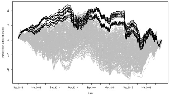
Figure 13.
Risk-adjusted returns (black lines) of the 72 minimum variance portfolios selected based on our proposed clustering procedure, compared to risk-adjusted returns (gray lines) of minimum variance portfolios constructed by all combinations (1001 in total) of four currencies out of total 14 currencies.
For a retrospective study, the performance of the proposed portfolios as well as all possible portfolios from 17 August 2016 to 10 September 2018 are plotted in Figure 14. Although these portfolios fail to be the best choices again, the resulting returns are still shown to have very strong invulnerability against fluctuations and risks.
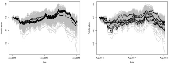
Figure 14.
Returns (black lines) of the selected minimum variance portfolios based on our clustering procedure (left, 72 portfolios in total) and the procedure proposed by De Luca and Zuccolotto (2011) (right, 32 portfolios in total). Each portfolio consists of four currencies, selected by choosing one currency from each of the four clusters, compared to returns (gray lines) of minimum variance portfolios constructed by all combinations (1001 in total) of four currencies out of total 14 currencies.
In contrast, in Figure 14, we also provide the paths of aggregate returns of all portfolios constructed by the method of De Luca and Zuccolotto (2011). Obviously, the performances are quite inconsistent and the returns seem to vary when volatility increases.
For the retrospective study, we also show the path of risk adjusted returns provided by our portfolios in Figure 15. The performance of our portfolios seems to be very good during early 2018 but relatively poor during late 2016 to 2017.
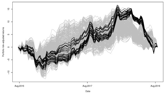
Figure 15.
Risk-adjusted returns (black lines) of the 72 minimum variance portfolios selected based on our proposed clustering procedure, compared to returns (gray lines) of minimum variance portfolios constructed by all combinations (1001 in total) of four currencies out of total 14 currencies.
6. Conclusions
In this paper, we have proposed a clustering procedure based on a new affinity measure indicating the extreme co-movements for financial time series. Unlike the common distance-based affinity matrix, our proposed affinity matrix is not necessarily symmetric and hence cannot be used as the input in hierarchical clustering algorithms directly. As a result, clustering procedures based on weighted cuts are employed and examined, and the WNACut method is finally selected as a recommended clustering procedure, based on the performances of compared procedures applicable. The resulting clusters seem to be reasonable when applied to the real exchange rate time series, and the portfolios constructed based on the resulting clusters are shown to outperform those from other clustering procedures, particularly in the long run.
Future research should focus on seeking consistent nonparametric estimators for the coefficients of maximal tail dependence such as WLTMD, since parametric copulas having explicit forms of these coefficients are not always available for the standard residuals extracted from the data. As pointed out in (Furman et al. 2015, sct. 7), the achievement in the area of M-estimators may be a possible way to obtain such estimators as well as the relevant statistical inference. Moreover, the idea of the OLS estimator (see Gabaix and Ibragimov 2011, for instance) may also be a potential way to address this challenging problem. Furthermore, as indexes of maximal tail dependence such as WLTMD are measures of extreme co-movements, they might not reflect the potential causality between quantities and hence could not be directly applied to some important issues in the financial markets such as contagion effects. Nevertheless, our proposed clustering procedure provides an insight to analyze financial time series using asymmetric information matrices such as matrices of contagion measures.
Supplementary Materials
The following are available at http://www.mdpi.com/2227-9091/6/4/115/s1, Table S1: 1001 portfolios constructed for all combinations of 4 currencies out of 14 currencies. The portfolio weights obtained by Markowitz minimal variance criteria is given in the bracket. Also, mean returns and accumulative returns are listed.
Author Contributions
Conceptualization, X.L.; Methodology, J.W.; Formal Analysis, C.Y.; Data Curation, W.J.
Funding
This research was funded by National Natural Science Foundation of China (71603190) and Ministry of Education in China (10YJC790280).
Conflicts of Interest
The authors declare no conflict of interest.
Appendix A. Proof of Proposition 2.1
Proof.
Since there exists a function such that
combined with the upper Fréchet–Hoeffding bound of copulas we must have for any ,
for all because . From Equation (A1), it is easy to obtain
Given the Lipschitz condition of copula, we have
as by noticing , then
for all . Combining Equations (A1) and (A3) yields
for all , and since , it further follows by Equations (A2) and (A4) that
for all . Provided the Karamata’s Representation Theorem, the slowly varying function has the following representation:
where measurable functions and satisfy
and
Hence, by Equation (A6), we have for all
Notice that, in Equation (A7), it is obvious that
the major discussion should focus on the limit of the rest part of Equation (A7) as . Since as , by defining for arbitrary we know that . Hence, for small enough , we could rewrite
Therefore, for all we have
which is equivalent to
Finally, combined with (A8) we deduce
Therefore, we may conclude that by letting for both inequalities of Equation (A9). ☐
Appendix B. Details of the Clustering Algorithm in Simulation
| Algorithm A1 Best WCut (Meilă and Pentney 2007, Algorithm 4.1). |
| Require: Affinity matrix, ; diagonal matrix of volume weights, ; diagonal matrix of row weights, ; number of clusters, k; Ensure: The clustering, ;
|
Appendix C. Goodness-of-Fit Test
Table A1.
Estimated Kolmogorov statistics for the goodness-of-fit test.
Table A1.
Estimated Kolmogorov statistics for the goodness-of-fit test.
| AUD | BRL | CAD | CNY | GBP | INR | IDR | JPY | KRW | MXN | RUB | ZAR | TRY | EUR | |
|---|---|---|---|---|---|---|---|---|---|---|---|---|---|---|
| AUD | — | 0.0634 | 0.0778 | 0.0636 | 0.0733 | 0.0614 | 0.0460 | 0.0747 | 0.0685 | 0.0922 | 0.0563 | 0.0815 | 0.0644 | 0.0487 |
| BRL | 0.0794 | — | 0.0685 | 0.0539 | 0.0425 | 0.0493 | 0.0488 | 0.0501 | 0.0527 | 0.0668 | 0.0766 | 0.0665 | 0.0841 | 0.0454 |
| CAD | 0.0899 | 0.0655 | — | 0.0502 | 0.0545 | 0.0512 | 0.0561 | 0.0673 | 0.0601 | 0.0568 | 0.0668 | 0.0563 | 0.0555 | 0.0629 |
| CNY | 0.0495 | 0.0445 | 0.0469 | — | 0.0794 | 0.0375 | 0.0633 | 0.0489 | 0.0666 | 0.0496 | 0.0494 | 0.0516 | 0.0516 | 0.0470 |
| GBP | 0.0603 | 0.0579 | 0.0517 | 0.0705 | — | 0.0481 | 0.0584 | 0.0580 | 0.0565 | 0.0493 | 0.0494 | 0.0486 | 0.0754 | 0.0414 |
| INR | 0.0633 | 0.0433 | 0.0470 | 0.0383 | 0.0484 | — | 0.0367 | 0.0476 | 0.0472 | 0.0290 | 0.0604 | 0.0462 | 0.0577 | 0.0637 |
| IDR | 0.0480 | 0.0531 | 0.0502 | 0.0612 | 0.0584 | 0.0371 | — | 0.0675 | 0.0686 | 0.0395 | 0.0577 | 0.0750 | 0.0665 | 0.0505 |
| JPY | 0.0687 | 0.0522 | 0.0677 | 0.0534 | 0.0611 | 0.0516 | 0.0705 | — | 0.0645 | 0.0637 | 0.0497 | 0.0513 | 0.0587 | 0.0542 |
| KRW | 0.0763 | 0.0619 | 0.0581 | 0.0797 | 0.0821 | 0.0569 | 0.0696 | 0.0643 | — | 0.0628 | 0.0578 | 0.0797 | 0.0896 | 0.0448 |
| MXN | 0.0861 | 0.0648 | 0.0748 | 0.0511 | 0.0524 | 0.0353 | 0.0353 | 0.0637 | 0.0543 | — | 0.0718 | 0.0585 | 0.0589 | 0.0446 |
| RUB | 0.0558 | 0.0748 | 0.0520 | 0.0550 | 0.0481 | 0.0493 | 0.0559 | 0.0485 | 0.0382 | 0.0512 | — | 0.0561 | 0.0565 | 0.0592 |
| ZAR | 0.0715 | 0.0620 | 0.0500 | 0.0566 | 0.0518 | 0.0504 | 0.0565 | 0.0510 | 0.0726 | 0.0786 | 0.0647 | — | 0.0687 | 0.0465 |
| TRY | 0.0675 | 0.0614 | 0.0542 | 0.0555 | 0.0890 | 0.0512 | 0.0599 | 0.0604 | 0.0719 | 0.0698 | 0.0576 | 0.0753 | — | 0.0483 |
| EUR | 0.0415 | 0.0574 | 0.0663 | 0.0483 | 0.0418 | 0.0607 | 0.0399 | 0.0548 | 0.0306 | 0.0339 | 0.0540 | 0.0419 | 0.0506 | — |
Appendix D. Economic Summary of G20 Nations
Table A2.
Part of the economic summary of G20 nations 2015 by (IMF (2014)).
Table A2.
Part of the economic summary of G20 nations 2015 by (IMF (2014)).
| Member | Nom. GDP mil. USD | PPP GDP mil. USD | Nom. GDP per capitaUSD | PPP GDP per capltaUSD | HDI | Population | Area | Economic Classification (IMF) |
|---|---|---|---|---|---|---|---|---|
| Argentina | 585,623 | 964,300 | 13,589 | 22,554 | 0.836 | 42,961,000 | 2,780,400 | Emerging |
| Australia | 1,223,887 | 1,489,000 | 50,962 | 47,389 | 0.935 | 23,599,000 | 7,692,024 | Advanced |
| Brazil | 1,772,589 | 3,166,000 | 8670 | 16,155 | 0.755 | 202,768,000 | 8,515,767 | Emerging |
| Canada | 1,552,386 | 1,632,000 | 43,332 | 44,967 | 0.913 | 35,467,000 | 9,984,670 | Advanced |
| China | 10,982,829 | 19,510,000 | 7990 | 14,107 | 0.727 | 1,367,520,000 | 9,572,900 | Emerging |
| France | 2,421,560 | 2,647,000 | 37,675 | 41,181 | 0.888 | 63,951,000 | 640,679 | Advanced |
| Germany | 3,357,614 | 3,842,000 | 40,997 | 46,893 | 0.916 | 80,940,000 | 357,114 | Advanced |
| India | 2,090,706 | 7,965,000 | 1617 | 6162 | 0.609 | 1,259,695,000 | 3,287,263 | Emerging |
| Indonesia | 858,953 | 2,839,000 | 3362 | 11,126 | 0.684 | 251,490,000 | 1,904,569 | Emerging |
| Italy | 1,815,757 | 2,174,000 | 29,867 | 35,708 | 0.873 | 60,665,551 | 301,336 | Advanced |
| Japan | 4,123,258 | 4,658,000 | 32,486 | 38,054 | 0.891 | 127,061,000 | 377,930 | Advanced |
| South Korea | 1,376,868 | 1,849,000 | 27,195 | 36,511 | 0.898 | 50,437,000 | 100,210 | Advanced |
| Mexico | 1,144,334 | 2,220,000 | 9009 | 17,534 | 0.756 | 119,581,789 | 1,964,375 | Emerging |
| Russia | 1,324,734 | 3,471,000 | 9055 | 25,411 | 0.798 | 146,300,000 | 17,098,242 | Emerging |
| Saudi Arabia | 653,219 | 1,683,000 | 20,813 | 53,624 | 0.837 | 30,624,000 | 2,149,690 | Emerging |
| South Africa | 312,957 | 723,518 | 5695 | 13,165 | 0.666 | 53,699,000 | 1,221,037 | Emerging |
| Turkey | 733,642 | 1,589,000 | 9437 | 20,438 | 0.761 | 77,324,000 | 783,562 | Emerging |
| United Kingdom | 2,849,345 | 2,660,000 | 43,771 | 41,159 | 0.907 | 64,511,000 | 242,495 | Advanced |
| United States | 17,947,000 | 17,947,000 | 55,805 | 55,805 | 0.915 | 318,523,000 | 9,526,468 | Advanced |
| European Union | 16,220,370 | 19,180,000 | 31,918 | 37,852 | 0.876 | 505,570,700 | 4,422,773 | N/A |
Appendix E. Seventy-Two Portfolios Constructed Based on Our Clustering Result in Table 7
Table A3.
Sevent-two portfolios constructed based on our clustering result in Table 7. Notice that for each cluster only one currency is selected. The portfolio weights obtained by Markowitz minimal variance criteria is given in the bracket. In addition, mean returns and accumulative returns are listed.
| Portfolio | Currency from Cluster 1 | Currency from Cluster 2 | Currency from Cluster 3 | Currency from Cluster 4 | Mean Return | Accumulative Return |
|---|---|---|---|---|---|---|
| 1 | AUD (0.0000) | BRL (0.0220) | CNY (0.9177) | JPY (0.0603) | −0.0321% | −6.6162% |
| 2 | CAD (0.0122) | BRL (0.0195) | CNY (0.9089) | JPY (0.0595) | −0.0329% | −6.7676% |
| 3 | GBP (0.0221) | BRL (0.0196) | CNY (0.8984) | JPY (0.0599) | −0.0333% | −6.8559% |
| 4 | EUR (0.0392) | BRL (0.0164) | CNY (0.8944) | JPY (0.0499) | −0.0313% | −6.4531% |
| 5 | AUD (0.0000) | INR (0.0539) | CNY (0.8841) | JPY (0.0620) | −0.0316% | −6.5051% |
| 6 | CAD (0.0188) | INR (0.0500) | CNY (0.8709) | JPY (0.0603) | −0.0332% | −6.8367% |
| 7 | GBP (0.0236) | INR (0.0508) | CNY (0.8643) | JPY (0.0613) | −0.0331% | −6.8180% |
| 8 | EUR (0.0419) | INR (0.0483) | CNY (0.8596) | JPY (0.0502) | −0.0315% | −6.4815% |
| 9 | AUD (0.0000) | IDR (0.0322) | CNY (0.9072) | JPY (0.0606) | −0.0320% | −6.5924% |
| 10 | CAD (0.0227) | IDR (0.0271) | CNY (0.8913) | JPY (0.0589) | −0.0336% | −6.9266% |
| 11 | GBP (0.0278) | IDR (0.0317) | CNY (0.8807) | JPY (0.0597) | −0.0340% | −6.9977% |
| 12 | EUR (0.0441) | IDR (0.0263) | CNY (0.8810) | JPY (0.0486) | −0.0315% | −6.4964% |
| 13 | AUD (0.0023) | MXN (0.0109) | CNY (0.9221) | JPY (0.0647) | −0.0299% | −6.1674% |
| 14 | CAD (0.0300) | MXN (0.0000) | CNY (0.9093) | JPY (0.0608) | −0.0310% | −6.3935% |
| 15 | GBP (0.0269) | MXN (0.0066) | CNY (0.9029) | JPY (0.0636) | −0.0310% | −6.3900% |
| 16 | EUR (0.0468) | MXN (0.0031) | CNY (0.8995) | JPY (0.0507) | −0.0288% | −5.9339% |
| 17 | AUD (0.0085) | ZAR (0.0000) | CNY (0.9290) | JPY (0.0626) | −0.0290% | −5.9725% |
| 18 | CAD (0.0300) | ZAR (0.0000) | CNY (0.9093) | JPY (0.0608) | −0.0310% | −6.3935% |
| 19 | GBP (0.0282) | ZAR (0.0000) | CNY (0.9091) | JPY (0.0627) | −0.0301% | −6.2074% |
| 20 | EUR (0.0476) | ZAR (0.0000) | CNY (0.9024) | JPY (0.0501) | −0.0284% | −5.8410% |
| 21 | AUD (0.0085) | TRY (0.0000) | CNY (0.9290) | JPY (0.0626) | −0.0290% | −5.9725% |
| 22 | CAD (0.0300) | TRY (0.0000) | CNY (0.9093) | JPY (0.0608) | −0.0310% | −6.3935% |
| 23 | GBP (0.0282) | TRY (0.0000) | CNY (0.9091) | JPY (0.0627) | −0.0301% | −6.2074% |
| 24 | EUR (0.0476) | TRY (0.0000) | CNY (0.9024) | JPY (0.0501) | −-0.0284% | −5.8410% |
| 25 | AUD (0.0000) | BRL (0.0264) | CNY (0.9736) | KRW (0.0000) | −0.0271% | −5.5828% |
| 26 | CAD (0.0217) | BRL (0.0218) | CNY (0.9566) | KRW (0.0000) | −0.0285% | −5.8756% |
| 27 | GBP (0.0234) | BRL (0.0238) | CNY (0.9528) | KRW (0.0000) | −0.0284% | −5.8427% |
| 28 | EUR (0.0606) | BRL (0.0166) | CNY (0.9228) | KRW (0.0000) | −0.0272% | −5.6042% |
| 29 | AUD (0.0045) | INR (0.0558) | CNY (0.9397) | KRW (0.0000) | −0.0262% | −5.3969% |
| 30 | CAD (0.0304) | INR (0.0511) | CNY (0.9185) | KRW (0.0000) | −0.0286% | −5.8954% |
| 31 | GBP (0.0260) | INR (0.0541) | CNY (0.9200) | KRW (0.0000) | −0.0275% | −5.6677% |
| 32 | EUR (0.0635) | INR (0.0480) | CNY (0.8885) | KRW (0.0000) | −0.0273% | −5.6167% |
| 33 | AUD (0.0058) | IDR (0.0391) | CNY (0.9516) | KRW (0.0036) | −0.0276% | −5.6778% |
| 34 | CAD (0.0321) | IDR (0.0346) | CNY (0.9332) | KRW (0.0000) | −0.0299% | −6.1540% |
| 35 | GBP (0.0303) | IDR (0.0416) | CNY (0.9282) | KRW (0.0000) | −0.0296% | −6.1004% |
| 36 | EUR (0.0643) | IDR (0.0307) | CNY (0.9050) | KRW (0.0000) | −0.0281% | −5.7784% |
| 37 | AUD (0.0143) | MXN (0.0000) | CNY (0.9762) | KRW (0.0094) | −0.0233% | −4.7940% |
| 38 | CAD (0.0418) | MXN (0.0000) | CNY (0.9581) | KRW (0.0001) | −0.0264% | −5.4331% |
| 39 | GBP (0.0289) | MXN (0.0000) | CNY (0.9621) | KRW (0.0089) | −0.0238% | −4.8943% |
| 40 | EUR (0.0690) | MXN (0.0000) | CNY (0.9310) | KRW (0.0000) | −0.0242% | −4.9823% |
| 41 | AUD (0.0143) | ZAR (0.0000) | CNY (0.9762) | KRW (0.0094) | −0.0233% | −4.7940% |
| 42 | CAD (0.0418) | ZAR (0.0000) | CNY (0.9581) | KRW (0.0001) | −0.0264% | −5.4331% |
| 43 | GBP (0.0289) | ZAR (0.0000) | CNY (0.9621) | KRW (0.0089) | −0.0238% | −4.8943% |
| 44 | EUR (0.0690) | ZAR (0.0000) | CNY (0.9310) | KRW (0.0000) | −0.0242% | −4.9823% |
| 45 | AUD (0.0143) | TRY (0.0000) | CNY (0.9762) | KRW (0.0094) | −0.0233% | −4.7940% |
| 46 | CAD (0.0418) | TRY (0.0000) | CNY (0.9581) | KRW (0.0001) | −0.0264% | −5.4331% |
| 47 | GBP (0.0289) | TRY (0.0000) | CNY (0.9621) | KRW (0.0089) | −0.0238% | −4.8943% |
| 48 | EUR (0.0690) | TRY (0.0000) | CNY (0.9310) | KRW (0.0000) | −0.0242% | −4.9823% |
| 49 | AUD (0.0000) | BRL (0.0264) | CNY (0.9736) | RUB (0.0000) | −0.0271% | −5.5828% |
| 50 | CAD (0.0217) | BRL (0.0218) | CNY (0.9566) | RUB (0.0000) | −0.0285% | −5.8756% |
| 51 | GBP (0.0234) | BRL (0.0238) | CNY (0.9528) | RUB (0.0000) | −0.0284% | −5.8427% |
| 52 | EUR (0.0606) | BRL (0.0166) | CNY (0.9228) | RUB (0.0000) | −0.0272% | −5.6042% |
| 53 | AUD (0.0045) | INR (0.0558) | CNY (0.9397) | RUB (0.0000) | −0.0262% | −5.3969% |
| 54 | CAD (0.0304) | INR (0.0511) | CNY (0.9185) | RUB (0.0000) | −0.0286% | −5.8954% |
| 55 | GBP (0.0260) | INR (0.0541) | CNY (0.9200) | RUB (0.0000) | −0.0275% | −5.6677% |
| 56 | EUR (0.0635) | INR (0.0480) | CNY (0.8885) | RUB (0.0000) | −0.0273% | −5.6167% |
| 57 | AUD (0.0071) | IDR (0.0394) | CNY (0.9534) | RUB (0.0000) | −0.0279% | −5.7458% |
| 58 | CAD (0.0321) | IDR (0.0346) | CNY (0.9332) | RUB (0.0000) | −0.0299% | −6.1540% |
| 59 | GBP (0.0303) | IDR (0.0416) | CNY (0.9282) | RUB (0.0000) | −0.0296% | −6.1004% |
| 60 | EUR (0.0643) | IDR (0.0307) | CNY (0.9050) | RUB (0.0000) | −0.0281% | −5.7784% |
| 61 | AUD (0.0182) | MXN (0.0000) | CNY (0.9818) | RUB (0.0000) | −0.0240% | −4.9542% |
| 62 | CAD (0.0418) | MXN (0.0000) | CNY (0.9582) | RUB (0.0000) | −0.0264% | −5.4349% |
| 63 | GBP (0.0310) | MXN (0.0000) | CNY (0.9690) | RUB (0.0000) | −0.0242% | −4.9888% |
| 64 | EUR (0.0690) | MXN (0.0000) | CNY (0.9310) | RUB (0.0000) | −0.0242% | −4.9823% |
| 65 | AUD (0.0182) | ZAR (0.0000) | CNY (0.9818) | RUB (0.0000) | −0.0240% | −4.9542% |
| 66 | CAD (0.0418) | ZAR (0.0000) | CNY (0.9582) | RUB (0.0000) | −0.0264% | −5.4349% |
| 67 | GBP (0.0310) | ZAR (0.0000) | CNY (0.9690) | RUB (0.0000) | −0.0242% | −4.9888% |
| 68 | EUR (0.0690) | ZAR (0.0000) | CNY (0.9310) | RUB (0.0000) | −0.0242% | −4.9823% |
| 69 | AUD (0.0182) | TRY (0.0000) | CNY (0.9818) | RUB (0.0000) | −0.0240% | −4.9542% |
| 70 | CAD (0.0418) | TRY (0.0000) | CNY (0.9582) | RUB (0.0000) | −0.0264% | −5.4349% |
| 71 | GBP (0.0310) | TRY (0.0000) | CNY (0.9690) | RUB (0.0000) | −0.0242% | −4.9888% |
| 72 | EUR (0.0690) | TRY (0.0000) | CNY (0.9310) | RUB (0.0000) | −0.0242% | −4.9823% |
References
- Bae, Kee-Hong, G. Andrew Karolyi, and Reneé M. Stulz. 2003. A New Approach to Measuring Financial Contagion. Review of Financial Studies 16: 717–63. [Google Scholar] [CrossRef]
- Baragona, Roberto. 2001. A simulation study on clustering time series with metaheuristic methods. Quaderni di Statistica 3: 1–26. [Google Scholar]
- Barberis, Nicholas, Andrei Shleifer, and Jeffrey Wurgler. 2005. Comovement. Journal of Financial Economics 75: 283–317. [Google Scholar] [CrossRef]
- Billio, Monica, and Massimiliano Caporin. 2009. A generalized Dynamic Conditional Correlation model for portfolio risk evaluation. Mathematics and Computers in Simulation 79: 2566–78. [Google Scholar] [CrossRef]
- Billio, Monica, Massimiliano Caporin, and Michele Gobbo. 2006. Flexible Dynamic Conditional Correlation multivariate GARCH models for asset allocation. Applied Financial Economics Letters 2: 123–30. [Google Scholar] [CrossRef]
- Bonanno, Giovanni, Guido Caldarelli, Fabrizio Lillo, Salvatore Miccichè, Nicolas Vandewalle, and Rosario N. Mantegna. 2004. Networks of equities in financial markets. The European Physical Journal B - Condensed Matter 38: 363–71. [Google Scholar] [CrossRef]
- Breymann, Wolfgang, Alexandra Dias, and Paul Embrechts. 2003. Dependence structures for multivariate high-frequency data in finance. Quantitative Finance 3: 1–14. [Google Scholar] [CrossRef]
- Brockwell, Peter J., and Richard A. Davis. 2002. Introduction to Time Series and Forecasting. Springer Texts in Statistics. New York: Springer. [Google Scholar] [CrossRef]
- Coles, Stuart, Janet Heffernan, and Jonathan Tawn. 1999. Dependence measures for extreme value analyses. Extremes 2: 339–65. [Google Scholar] [CrossRef]
- De Luca, Giovanni, and Paola Zuccolotto. 2011. A tail dependence-based dissimilarity measure for financial time series clustering. Advances in Data Analysis and Classification 5: 323–40. [Google Scholar] [CrossRef]
- De Luca, Giovanni, and Paola Zuccolotto. 2015. Dynamic tail dependence clustering of financial time series. Statistical Papers 58: 641–57. [Google Scholar] [CrossRef]
- Durante, Fabrizio, Enrico Foscolo, Piotr Jaworski, and Hao Wang. 2014. A spatial contagion measure for financial time series. Expert Systems with Applications 41: 4023–34. [Google Scholar] [CrossRef]
- Durante, Fabrizio, Roberta Pappadà, and Nicola Torelli. 2014. Clustering of financial time series in risky scenarios. Advances in Data Analysis and Classification 8: 359–76. [Google Scholar] [CrossRef]
- Durante, Fabrizio, Roberta Pappadà, and Nicola Torelli. 2015. Clustering of time series via non-parametric tail dependence estimation. Statistical Papers 56: 701–21. [Google Scholar] [CrossRef]
- Engle, Robert. 2002. Dynamic Conditional Correlation: A Simple Class of Multivariate Generalized Autoregressive Conditional Heteroskedasticity Models. Journal of Business & Economic Statistics 20: 339–50. [Google Scholar]
- Engle, Robert, and Kevin Sheppard. 2001. Theoretical and Empirical properties of Dynamic Conditional Correlation Multivariate GARCH. Cambridge: National Bureau of Economic Research. [Google Scholar] [CrossRef]
- International Monetary Fund. 2014. World Economic Outlook Database. Washington: International Monetary Fund. [Google Scholar]
- Furman, Edward, Alexey Kuznetsov, Jianxi Su, and Ričardas Zitikis. 2016. Tail dependence of the Gaussian copula revisited. Insurance: Mathematics and Economics 69: 97–103. [Google Scholar]
- Furman, Edward, Jianxi Su, and Ričardas Zitikis. 2015. Paths and indices of maximal tail dependence. ASTIN Bulletin 45: 661–78. [Google Scholar] [CrossRef]
- Gabaix, Xavier, and Rustam Ibragimov. 2011. Rank −1/2: A Simple Way to Improve the OLS Estimation of Tail Exponents. Journal of Business & Economic Statistics 29: 24–39. [Google Scholar]
- Hua, Lei, and Harry Joe. 2011. Tail order and intermediate tail dependence of multivariate copulas. Journal of Multivariate Analysis 102: 1454–71. [Google Scholar] [CrossRef]
- Kaufman, Leonard, and Peter J. Rousseeuw. 1990. Finding Groups in Data: An Introduction to Cluster Analysis. Wiley Series in Probability and Statistics; Hoboken: John Wiley & Sons, Inc. [Google Scholar] [CrossRef]
- Liebscher, Eckhard. 2008. Construction of asymmetric multivariate copulas. Journal of Multivariate Analysis 99: 2234–50. [Google Scholar] [CrossRef]
- Mantegna, Rosario N. 1999. Hierarchical structure in financial markets. The European Physical Journal B 11: 193–97. [Google Scholar] [CrossRef]
- Meilă, Marina. 2003. Comparing Clusterings by the Variation of Information. In Learning Theory and Kernel Machines. Berlin and Heidelberg: Springer Nature Switzerland AG, pp. 173–87. [Google Scholar] [CrossRef]
- Meilă, Marina, and William Pentney. 2007. Clustering by weighted cuts in directed graphs. Paper presented at 2007 SIAM International Conference on Data Mining, Philadelphia, PA, USA, 26–28 April. [Google Scholar]
- Nelsen, Roger B. 2006. An Introduction to Copulas. Springer Series in Statistics; New York: Springer. [Google Scholar] [CrossRef]
- Pericoli, Marcello, and Massimo Sbracia. 2003. A Primer on Financial Contagion. Journal of Economic Surveys 17: 571–608. [Google Scholar] [CrossRef]
- Veldkamp, Laura L. 2006. Information markets and the comovement of asset prices. The Review of Economic Studies 73: 823–45. [Google Scholar] [CrossRef]
- Verma, Deepak, and Marina Meilă. A Comparison of Spectral Clustering Algorithms. Technical Report UW-CSE-03-05-01. Seattle: University of Washington.
| 1 | The currencies include: Argentine Pesos, Australian Dollars, Brazilian Reals, British Pounds, Canadian Dollars, Chinese Renminbi, European Euros, Indian Rupees, Indonesian Rupiah, Japanese Yen, Mexican Pesos, Russian Rubles, Saudi Arabian Riyal, South African Rand, South Korean Won, and Turkish New Lira. |
© 2018 by the authors. Licensee MDPI, Basel, Switzerland. This article is an open access article distributed under the terms and conditions of the Creative Commons Attribution (CC BY) license (http://creativecommons.org/licenses/by/4.0/).