Numerical Ruin Probability in the Dual Risk Model with Risk-Free Investments

Abstract

In this paper, a dual risk model under constant force of interest is considered. The ruin probability in this model is shown to satisfy an integro-differential equation, which can then be written as an integral equation. Using the collocation method, the ruin probability can be well approximated for any gain distributions. Examples involving exponential, uniform, Pareto and discrete gains are considered. Finally, the same numerical method is applied to the Laplace transform of the time of ruin.

1. Introduction

The simplest surplus model in non-life insurance is known as the Cramér–Lundberg model or the classical risk model. It assumes that the company collects premiums at a fixed rate and pays out claims of a random amount at random times. Mathematically, the surplus process can be written as:

$$U_t=u+ct-\sum _{k=1}^{N_t}{X}_k,$$

(1)

where u is the initial capital, c is the constant premium rate, $X_1,X_2,\dots$ are the claim sizes and $N_t$ is the claim arrival process, which counts the number of claims in the time interval $[0,t]$. It is vital for any company to operate above a certain income level. For convenience, this level is set to be zero. Define the time of ruin by:

$$\tau =inf\{s>0\mid U_s<0\},$$

where if $U_s\ge 0$ for all s, then $\tau =inf\varnothing =\infty .$ Define the ruin probability with initial surplus $U_0=u$ by:

$$\psi (u)=P(\tau <\infty \mid U_0=u).$$

The classical model (1) assumes that the only source of income is from collecting premiums. In the past, many models incorporated investments with constant force of interest, for example, investing all (or part) of the surplus in bonds or time accounts. The study of these risk models dated back to Segerdahl (1942), who considered the constant interest risk model and provided an explicit expression for the ruin probability when the claims are exponentially distributed. Sundt and Teugels (1995) gave an extensive treatment of the ruin probability with constant interest force and obtained approximations, as well as upper and lower bounds. Kasozi and Paulsen (2005) used numerical methods such as the block-by-block method and the Simpson rule to approximate the ultimate ruin probabilities under a constant rate of interest. Cai et al. (2009) considered the well-known Gerber–Shiu function under the risk model of liquid reserves and constant interest on the surplus, and more recently, Schmidli (2015) studied a variant of the discounted penalty function where a penalty applies when the surplus process leaves a finite interval. Yang and Wang (2010) investigated the asymptotic behavior of the ruin probability of some negatively dependent risk models with a constant interest rate and dominatedly-varying-tailed claims. Renewal risk models with constant interest were well studied by Konstantinides et al. (2010).

A dual model to (1) is obtained by regarding premiums as expenses and claims as gains. In life annuity insurance or pension insurance, a basic model for the surplus process is known as the classical dual risk model, which is given by:

$$U_t=u-ct+\sum _{k=1}^{N_t}{X}_k.$$

(2)

Here, c denotes the expense rate, $\left\{X_k\right\}$ represent random gains and $N_t$ is called the gain arrival process. The process $N_t$ is assumed to be a homogenous Poisson process with intensity $\lambda >0$. Moreover, it is assumed that the claim sizes $X_1,X_2,\dots$ are independent and identically distributed (i.i.d) with cumulative distribution function (c.d.f.) F and tail distribution function $\overline{F}=1-F$ and that the processes $\left\{X_i\right\}$ and $N_t$ are independent.

Therefore, (2) models the surplus process of a company with a constant rate of consumption, earning random income at random times. Other examples of such companies are non-profit organizations and petroleum companies where the jumps correspond to random donations (see Chen (2010)) and discoveries of oil (see Avanzi et al. (2007)), respectively. Throughout this paper, the terms “gains”, “innovations” and “donations” will be used interchangeably.

Contrary to the vast literature on the insurance models, there were very few results published in the dual model with constant force of interest. Zeng and Xu (2013) considered the perturbed dual risk model with constant interest and a threshold dividend strategy. They used the sinc method to approximate the expected present value of total dividends. Dong and Wang (2008) studied the renewal risk model with constant force of interest and obtained an explicit expression for the ruin probability in terms of infinite series of iterated integrals. Although their renewal model is more general than the Poisson process considered here, the objective and approach of this paper differ from Dong and Wang (2008).

Here, the main objective is to examine the ruin probability numerically in the dual risk model with risk-free investments under an arbitrary gain distribution. Section 2 shows the derivation of the integro-differential equation (IDE) that is satisfied by ruin probability. From the IDE, Section 3 carefully demonstrates that the derivative of the ruin probability satisfies an integral equation (IE). The ruin probability for certain gain sizes (such as exponential and a mixture of exponentials) has a very explicit representation. In Section 4, using the collocation method, the IE is reduced to a linear matrix equation. The ruin probability can then be obtained numerically for any jump distributions. For numerical illustrations, exponential, uniform, Pareto and discrete gains are considered. In Section 5, the same numerical method is applied to other functionals of the time of ruin, such as the Laplace transform of the ruin time. Exponential gains are again considered to illustrate the numerical scheme. Finally, Section 6 concludes the findings of this paper.

2. The Model

All assumptions in the classical dual model (2) are retained, and it is further assumed that the company invests all of its surplus in a risk-free asset with constant force of interest $a>0$. The surplus process can now be written as:

$$U_t=u-ct+a{\int }_0^t{U}_{s}ds+\sum _{i=1}^{N_t}{X}_i.$$

(3)

Define the consumption (or investment) process $\left\{Z_t\right\}$ by:

$$Z_t=u-ct+a{\int }_0^t{Z}_{s}ds,$$

or equivalently, in differential form,

$$d{Z}_t=(a{Z}_t-c)dt,Z_0=u.$$

Observe that $\left\{Z_t\right\}$ is a deterministic process and that the above is an ordinary differential equation (ODE) with solution:

$$Z_t=\left(u-\frac{c}{a}\right)e^{at}+\frac{c}{a},t\ge 0.$$

Since $Z_t\ge 0$ for all t whenever $u\ge \frac{c}{a}$, one has:

$$\psi (u)=0\mathrm{for}\mathrm{all}u\ge \frac{c}{a}.$$

(4)

In other words, if the initial capital is greater than $\frac{c}{a}$, the contribution from the risk-free investments always offsets the expenses, and so, the company can never be ruined. Hence, for the ruin probability $\psi (u)$, only values of u between zero and $\frac{c}{a}$ are of interest.

Theorem 1.

Assume that the ruin probability $\psi (u)$ is differentiable. For $0<u<\frac{c}{a}$, the ruin probability satisfies the IDE:

$$(au-c){\psi }^{\prime }(u)-\lambda \psi (u)+\lambda {\int }_0^{c/a-u}\psi (u+x)dF(x)=0,$$

(5)

with boundary conditions:

$$\psi (0)=1\mathit{and}\psi \left(\frac{c}{a}\right)=0.$$

(6)

Proof. 

Consider the risk process $U_t$ in an infinitesimal time interval $(0,h)$ where $h<\frac{1}{a}\left|\ln \frac{c}{c-au}\right|$. Therefore,

$$\begin{array}{cc}\hfill \psi (u)& =\mathbb{E}({\mathrm{𝟙}}_{[\tau <\infty ]}{\mathrm{𝟙}}_{[N(h)=0]}\mid U_0=u)+\mathbb{E}({\mathrm{𝟙}}_{[\tau <\infty ]}{\mathrm{𝟙}}_{[N(h)=1]}\mid U_0=u)+\mathbb{E}({\mathrm{𝟙}}_{[\tau <\infty ]}{\mathrm{𝟙}}_{[N(h)>1]}\mid U_0=u)\hfill \\ & =e^{-\lambda h}\psi (Z_h)+{\int }_0^h\lambda e^{-\lambda s}{\int }_0^{c/a-Z_s}\psi (Z_s+x)dF(x)ds+o(h).\hfill \end{array}$$

(7)

By the chain rule,

$$\underset{h\to 0}{lim}\frac{\psi (Z_h)-\psi (u)}{h}={\psi }^{\prime }(u)·a(u-c/a).$$

Dividing (7) by h and taking the limit as $h\to 0$, one obtains:

$$0=(au-c){\psi }^{\prime }(u)e^0+\psi (u)·(-\lambda )+\lambda e^0{\int }_0^{c/a-u}\psi (u+x)dF(x).$$

 □

Remark 1.

Theorem 1 coincides with Equation (20) in Dong and Wang (2008) when $n=1$.

Remark 2.

In the classical risk model with risk-free investments, it has been proven that the ruin probability is continuously differentiable on the positive real line, except at points of discontinuity of the jump distribution (for example, see Mishura and Ragulina (2016), Chapter 2, and the references therein). One can verify that the same is true for the dual model considered in this paper.

3. Integral Equation Approach

Here, the derivative of $\psi$ is shown to satisfy a simple integral equation. This provides a framework for the numerical approximation of the ruin probability in the next section.

For $u\ge 0$, define:

$$\chi (u)\equiv \left\{\begin{array}{cc}{\psi }^{\prime }(u),\hfill & \hfill 0\le u\le \frac{c}{a},\\ 0,\hfill & \hfill u>\frac{c}{a}.\end{array}\right.$$

Using (4), for $0\le u\le \frac{c}{a}$, we have:

$$\begin{array}{cc}\hfill \psi (u)-{\int }_0^{c/a-u}\psi (u+x)dF(x)& ={\int }_0^{c/a-u}(\psi (u)-\psi (u+x))dF(x)+{\int }_{c/a-u}^{\infty }(\psi (u)-0)dF(x)\hfill \\ & ={\int }_0^{\infty }{\int }_{u+x}^u\chi (t)dtdF(x)\hfill \\ & =-{\int }_u^{\infty }\overline{F}(t-u)\chi (t)dt.\hfill \end{array}$$

Therefore, the IDE (5) becomes an IE given by:

$$(au-c)\chi (u)=-\lambda {\int }_u^{c/a}\overline{F}(t-u)\chi (t)dt,0<u<\frac{c}{a}.$$

Denoting $\frac{c}{a}=b$ and $\frac{\lambda }{a}=d$, the above IE can be rewritten as:

$$\chi (u)=\frac{d}{b-u}{\int }_u^b\overline{F}(t-u)\chi (t)dt,0<u<b,$$

(8)

with the integrability condition:

$${\int }_0^b\chi (u)du=\psi (b)-\psi (0)=-1.$$

(9)

Performing the change of variable $\chi (u)={(b-u)}^{d-1}\tilde{\chi }(u)$, (8) becomes:

$${(b-u)}^{d-1}\tilde{\chi }(u)=\frac{d}{b-u}{\int }_u^b\overline{F}(t-u){(b-t)}^{d-1}\tilde{\chi }(t)dt,0<u<b.$$

Therefore,

$$\begin{array}{cc}\hfill {(b-u)}^d\tilde{\chi }(u)& =-{\int }_u^b\overline{F}(t-u)\tilde{\chi }(t)\frac{d}{dt}{(b-t)}^{d}dt\hfill \\ & =\overline{F}(t-u)\tilde{\chi }(t){(b-t)}^d{\mid }_b^u+{\int }_u^b{(b-t)}^d\frac{d}{dt}\left[\overline{F}(t-u)\tilde{\chi }(t)\right]dt,\hfill \end{array}$$

and so, one obtains:

$$0={\int }_u^b{(b-t)}^d\frac{d}{dt}\left[\overline{F}(t-u)\tilde{\chi }(t)\right]dt,0<u<b.$$

(10)

The IE (10) can now be used to obtain numerical approximations for any arbitrary jump distributions. In certain cases, the explicit expression of $\psi$ is simple enough, and this can be used to validate the numerical approximation in the next section.

Example 1.

Assume that the gains are exponentially distributed with mean μ, that is, $\overline{F}(x)=e^{-x/\mu }$. Then, (10) reduces to:

$$0=e^{u/\mu }{\int }_u^b{(b-t)}^d\frac{d}{dt}\left[e^{-t/\mu }\tilde{\chi }(t)\right]dt.$$

Since the above holds for all u, the integral term must be equal to zero. Differentiating this equation leads to the ODE ${\tilde{\chi }}^{\prime }(u)-\frac{1}{\mu }\tilde{\chi }(u)=0,$ with the solution given by $\tilde{\chi }(u)=e^{u/\mu }.$ Therefore,

$$\chi (u)={(b-u)}^{\lambda /a-1}{e}^{u/\mu }$$

and the boundary conditions (6) are then used to obtain:

$$\psi (u)=\frac{\Gamma (\frac{\lambda }{a},0)-\Gamma (\frac{\lambda }{a},\frac{c-au}{a\mu })}{\Gamma (\frac{\lambda }{a},0)-\Gamma (\frac{\lambda }{a},\frac{c}{a\mu })},0\le u\le c/a,$$

(11)

where $\Gamma (b,x):={\int }_x^{\infty }{t}^{b-1}{e}^{-t}dt$ is the incomplete Gamma function.

Example 2.

Assume that the gains are distributed as a mixture of two exponentials, i.e., $\overline{F}(x)=p{e}^{-{\mu }_{1}x}+(1-p)e^{-{\mu }_{2}x}$ where w.l.o.g. ${\mu }_1>{\mu }_2$ and $0\le p<1$. Then, (10) can be written as:

$$\begin{array}{cc}\hfill 0& =p{e}^{{\mu }_{1}u}{\int }_u^b{(b-t)}^d\frac{d}{dt}\left[e^{-{\mu }_{1}t}\tilde{\chi }(t)\right]dt+(1-p)e^{{\mu }_{2}u}{\int }_u^b{(b-t)}^d\frac{d}{dt}\left[e^{-{\mu }_{2}t}\tilde{\chi }(t)\right]dt.\hfill \end{array}$$

(12)

Differentiating (12) twice and simplifying yield a second order linear ODE:

$$(b-u){\tilde{\chi }}^{″}(u)-((b-u)({\mu }_1+{\mu }_2)+d){\tilde{\chi }}^{\prime }(u)+({\mu }_1{\mu }_2(b-u)+d({\mu }_{1}p+{\mu }_2(1-p)))\tilde{\chi }(u)=0.$$

From Polyanin and Zaitsev (2002), the general solution to the above ODE is given by:

$$\tilde{\chi }(u)=c_1{e}^{{\mu }_{1}u}{}_1{F}_1(d(1-p),d,({\mu }_1-{\mu }_2)(b-u))+c_2{e}^{{\mu }_{1}u}U(d(1-p),d,({\mu }_1-{\mu }_2)(b-u)),$$

where ${}_1{F}_1$ and U are the confluent hypergeometric functions (see Slater (1960)) and $c_1$, $c_2$ are arbitrary constants. Therefore, the ruin probability is given by:

$$\psi (u)=1-c_1{\int }_0^u{\Psi }_1(s)ds-c_2{\int }_0^u{\Psi }_2(s)ds,$$

where:

$$\begin{array}{cc}\hfill {\Psi }_1(u)& =e^{{\mu }_{1}u}{\left(\frac{c}{a}-u\right)}^{\lambda /a-1}{}_1{F}_1\left(\frac{(1-p)\lambda }{a},\frac{\lambda }{a},({\mu }_1-{\mu }_2)\left(\frac{c}{a}-u\right)\right),\hfill \\ \hfill {\Psi }_2(u)& =e^{{\mu }_{1}u}{\left(\frac{c}{a}-u\right)}^{\lambda /a-1}U\left(\frac{(1-p)\lambda }{a},\frac{\lambda }{a},({\mu }_1-{\mu }_2)\left(\frac{c}{a}-u\right)\right).\hfill \end{array}$$

The boundary conditions are then used to determine the constants $c_1$ and $c_2$, as shown in Dong and Wang (2008).

Remark 3.

In general, an explicit expression for ψ can be obtained if the c.d.f. of the gains satisfies an ODE with constant coefficients. The techniques used in Examples 1 and 2 can be applied to the case of the mixture of n exponentials, i.e., $\overline{F}(x)={\sum }_{i=1}^n{p}_i{e}^{-{\mu }_{i}x}$ where $0\le p_i<1$ with ${\sum }_{i=1}^n{p}_i=1$, which is an important class of distributions since any positive distributions can be approximated by the mixture of exponentials. If the c.d.f. is not of this form, e.g., uniform or Pareto gains, explicit formulas are difficult to obtain. This leads to the next section, which provides numerical approximations for ψ under arbitrary gains.

4. Numerical Scheme

In this section, a numerical framework for the ruin probability under any gain distributions is presented. The numerical scheme requires solving a simple linear system $A\tilde{\chi }=Y$ where A and Y are to be determined and the vector $\tilde{\chi }$ consists of values of the function $\tilde{\chi }(u)$ evaluated at some discrete points.

Consider the partition $0=u_0<u_1<\cdots <u_{N-1}<u_N=b$. For each $j=1,\dots ,N-1$, (10) can be written as:

$$0={\int }_{u_j}^b{(b-t)}^d\frac{d}{dt}[\overline{F}(t-u_j)\tilde{\chi }(t)]dt.$$

For each fixed $u_j$, discretize in the t variable where the length of $\Delta t$ coincides with the length of $\Delta u$. The derivative term is approximated using the forward difference method. Defining ${\tilde{\chi }}_i\approx \tilde{\chi }(u_i)$, one arrives at the following system of equations:

$$0=\sum _{k=j}^{N-1}{(b-u_k)}^d\left[\overline{F}(u_{k+1}-u_j){\tilde{\chi }}_{k+1}-\overline{F}(u_k-u_j){\tilde{\chi }}_k\right],j=1,\dots ,N-1,$$

which can be rewritten as:

$$0=-{(b-u_j)}^d{\tilde{\chi }}_j+\sum _{k=j+1}^N\overline{F}(u_k-u_j){\tilde{\chi }}_k[{(b-u_{k-1})}^d-{(b-u_k)}^d],j=1,\dots ,N-1.$$

The integrability condition (9) is approximated by:

$$\sum _{i=1}^{N-1}{(b-u_i)}^{d-1}{\tilde{\chi }}_i=-1.$$

Therefore, one obtains the matrix equation:

$$A\tilde{\chi }=Y,$$

(13)

where $\tilde{\chi }={[{\tilde{\chi }}_1,\cdots ,{\tilde{\chi }}_N]}^T$, $Y={[0,\cdots ,0,1]}^T$, and $A=(a_{jk})$ where:

$$a_{jk}=\left\{\begin{array}{cc}\overline{F}(u_k-u_j)[{(b-u_{k-1})}^d-{(b-u_k)}^d],\hfill & \hfill j=1,\dots ,N-1,k=j+1,\dots ,N\\ -{(b-u_j)}^d,\hfill & \hfill j=1,\dots ,N-1,k=j,\\ -{(b-u_k)}^{d-1},\hfill & \hfill j=N,k=1,\dots ,N-1,\\ 0\hfill & \hfill \mathrm{else}.\end{array}\right.$$

(14)

To solve (13), the matrix A needs to be invertible. The following lemma asserts this claim.

Lemma 1.

If B is an $N\times N$ matrix of the form:

$$B=\left[\begin{array}{ccccc}-b_{1,1}& b_{1,2}& \dots & b_{1,N-1}& b_{1,N}\\ 0& -b_{2,2}& \dots & b_{2,N-1}& b_{2,N}\\ ⋮& ⋮& \ddots & ⋮& ⋮\\ 0& 0& \dots & -b_{N-1,N-1}& b_{N-1,N}\\ -b_{N,1}& -b_{N,2}& \dots & -b_{N,N-1}& 0\end{array}\right],$$

where each $b_{j,k}>0$, then $det(B)\ne 0$.

Proof. 

It suffices to show that B can be reduced, using elementary row operations, to an upper triangular matrix with non-zero diagonal entries. First, perform $R_1\leftarrow R_1-\frac{b_{1,1}}{b_{N,1}}{R}_N$, which results in a matrix with the first row of the form $[0b_{1,2}^{\prime }\cdots b_{1,N-1}^{\prime }{b}_{1,N}]$ where each $b_{1,k}^{\prime }$ is positive. Inductively, perform the row operations $R_1\leftarrow R_1+\frac{b_{1,j}^{\prime }}{b_{j,j}}{R}_j$ for each $j=2,\dots ,N-1$. These operations result in a matrix with the first row of the form $[00\cdots 0b^{*}]$ where $b^{*}>0$. Finally, swap the first row with the last row to obtain an upper triangular matrix with non-zero diagonal entries. □

Thus, $\tilde{\chi }=A^{-1}Y$. To recover $\chi$, for each $j=1,\dots ,N-1$, multiply the j-th component of $\tilde{\chi }$ by ${(b-u_j)}^{d-1}$. Since $\chi ={\psi }^{\prime }$, performing the numerical integration:

$${\psi }_j=\sum _{k=j}^N{\chi }_i$$

yields the vector $\psi \equiv {[{\psi }_1,\cdots ,{\psi }_N]}^T$ where ${\psi }_i\approx \psi (u_i)$. Finally, the vector $\psi$ is normalized by imposing the boundary condition $\psi (0)=1$.

The following four examples show the approximate ruin probabilities under different gain distributions. Naturally, the first example concerns the exponentially-sized gains.

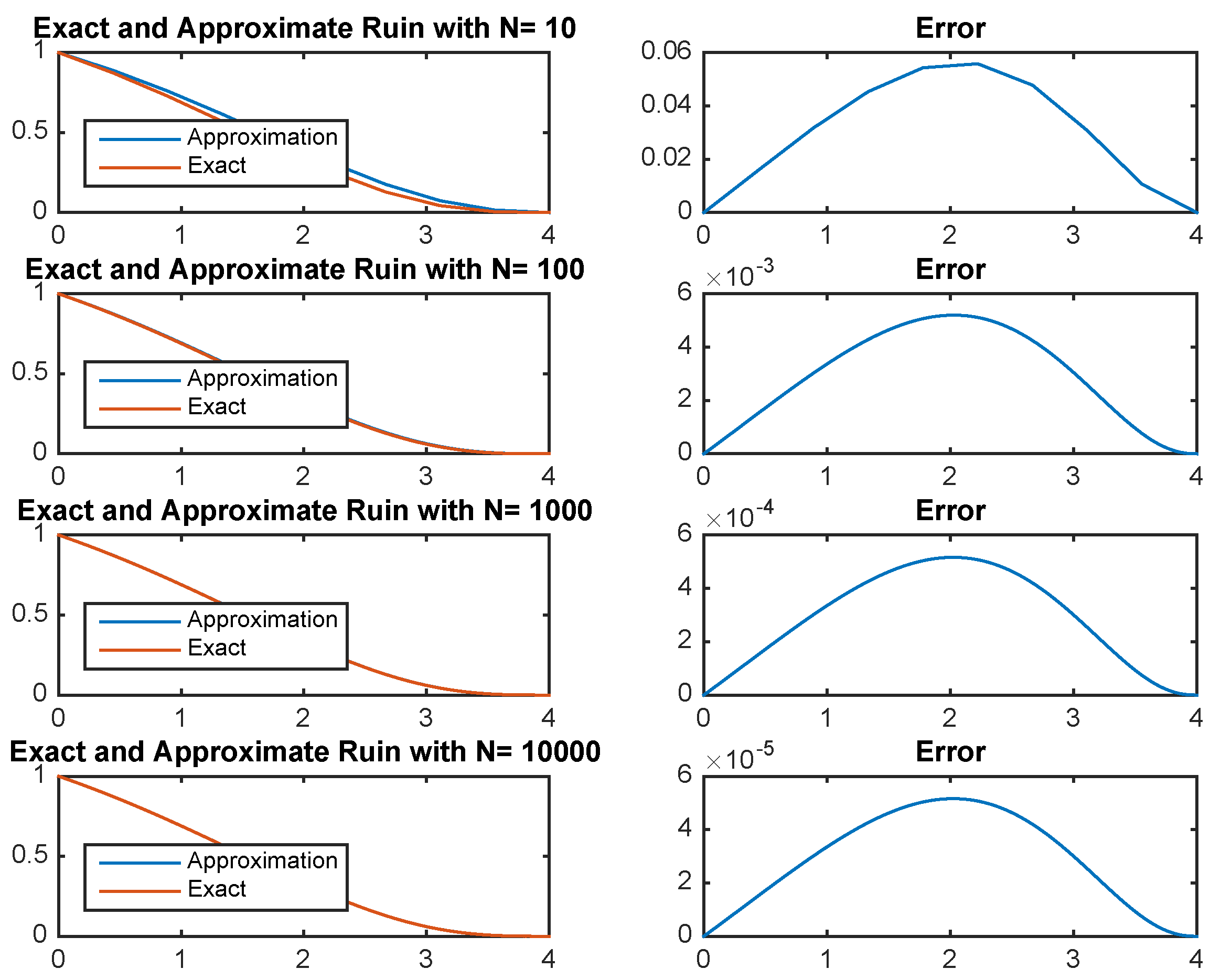
Example 3.

Suppose that $\overline{F}(x)=e^{-x}$. Let $\frac{c}{a}=b=4$ and $\frac{\lambda }{a}=d=3.5$. From Example 1,

$$\psi (u)=\frac{\Gamma (1.5,0)-\Gamma (1.5,4-u)}{\Gamma (1.5,0)-\Gamma (1.5,4)}.$$

Figure 1 shows that the numerical approximation of ψ approaches the exact solution as the number of subintervals increases. The maximum error is used for error analysis, which is the largest absolute difference between the approximation and the true value of ψ. The resulting error suggests that this numerical scheme has a first order of accuracy, which is unsurprising since first order discretization is used for the integral term, as well as for the derivative term.

The next three examples concern gains with c.d.f. that does not satisfy any ODE with constant coefficients, and so, the exact expression for the ruin probability is complicated. In all three examples, varying one of the parameters in the model leads to some interesting yet intuitive results.

Example 4.

Consider uniformly distributed gains on the interval $[0,\theta ]$. Then,

$$\overline{F}(x)=\left\{\begin{array}{cc}1,\hfill & \hfill x\le 0\\ 1-\frac{x}{\theta },\hfill & \hfill 0<x\le \theta \\ 0,\hfill & \hfill x>\theta .\end{array}\right.$$

For the numerical experiment, set $\frac{c}{a}=b=4$, $\frac{\lambda }{a}=d=1.5$ and $N=100$. Figure 2 shows that the numerical approximation of ψ approaches a limiting curve as the parameter θ increases.

This limiting curve can be found by investigating the IDE (5). For each parameter θ, denote the associated ruin probability by ${\psi }_{\theta }$. Then, the IDE is given by:

$$(au-c){\psi }_{\theta }^{\prime }(u)-\lambda {\psi }_{\theta }(u)+\lambda {\int }_0^{c/a-u}\frac{1}{\theta }{\mathrm{𝟙}}_{[0<x<\theta ]}{\psi }_{\theta }(u+x)dx=0.$$

Now,

$$\frac{\lambda }{\theta }{\int }_0^{c/a-u}{\mathrm{𝟙}}_{[0<x<\theta ]}{\psi }_{\theta }(u+x)dx=\frac{\lambda }{\theta }{\int }_u^{min\{c/a,\theta \}}{\psi }_{\theta }(y)dy\to 0$$

as $\theta \to \infty$ by the dominated convergence theorem since $0\le {\psi }_{\theta }\le 1$. Hence, as $\theta \to \infty$, the IDE becomes:

$$(au-c){\psi }_{\infty }^{\prime }(u)-\lambda {\psi }_{\infty }(u)=0,$$

and so, the solution of the above that satisfies the boundary conditions (6) is given by:

$${\psi }_{\infty }(u)={\left(1-\frac{u}{b}\right)}^{\lambda /a},0<u<b.$$

Observe that there is a natural monotonicity in this case. If ${\theta }_1<{\theta }_2$, then ${\psi }_{{\theta }_1}(u)>{\psi }_{{\theta }_2}(u)$ for all $0<u<b$. This property agrees with the model, since larger gains will reduce the probability of ruin.

The next example features a heavy tail gain distribution.

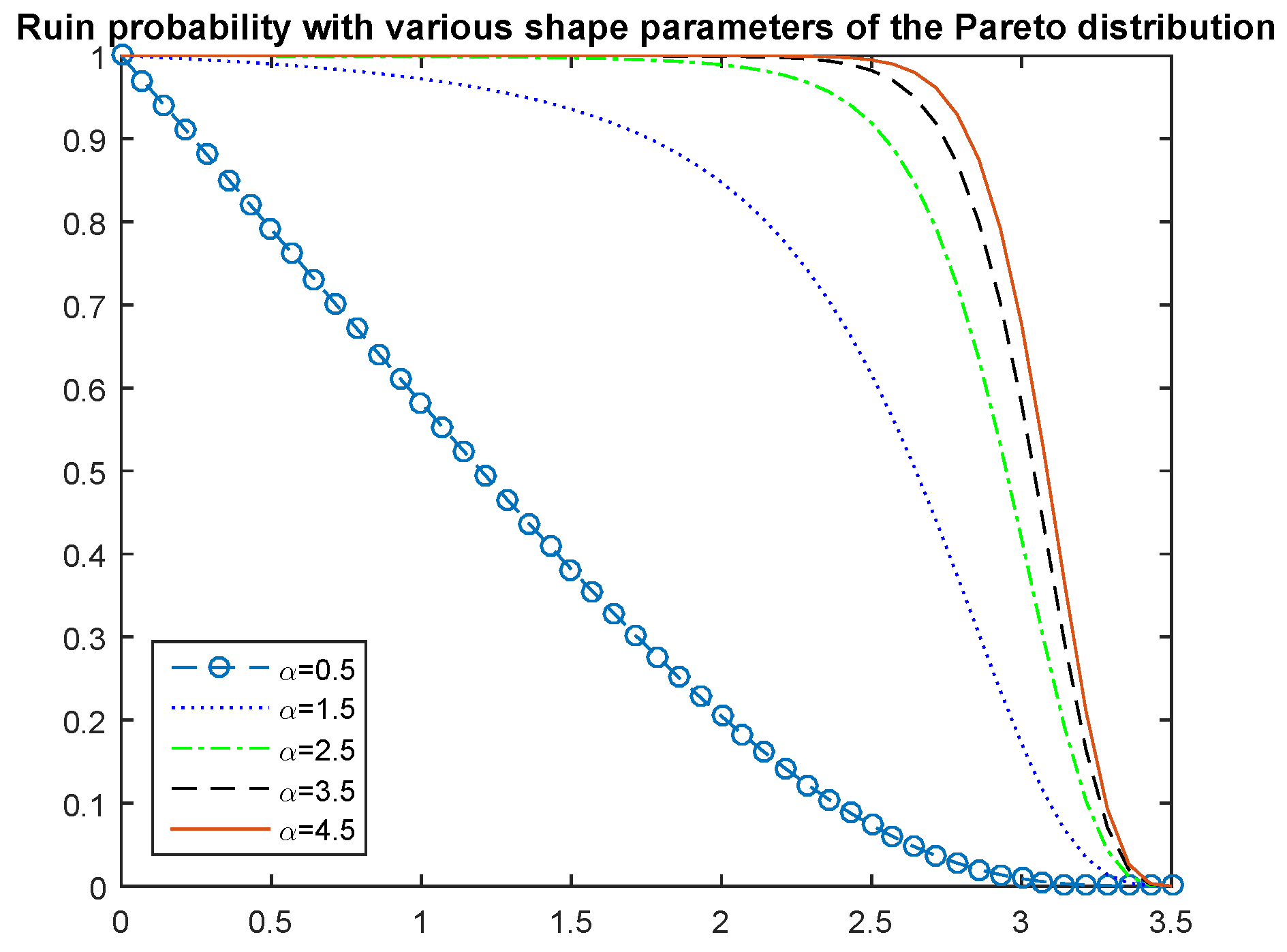
Example 5.

Suppose that the gains follow a Pareto distribution, whose tail distribution is given by:

$$\overline{F}(x)=\left\{\begin{array}{cc}1,\hfill & \hfill x\le x_m\\ {\left(\frac{x_m}{x}\right)}^{\alpha },\hfill & \hfill x>x_m.\end{array}\right.$$

For the numerical illustration, set $\frac{c}{a}=b=4$, $\frac{\lambda }{a}=d=3.5$ and $N=100$. Figure 3 shows that the numerical approximation of ψ approaches a limiting curve as the parameter α increases.

The limiting function can be thought of as follows. As $\alpha \to \infty$, X converges to a constant random variable $x_m$, that is the p.d.f. $f(x)\to {\delta }_{x_m}$. Hence, from the IDE (5), one obtains the following delay differential equation (DDE):

$$\begin{array}{cc}\hfill (au-c){\psi }^{\prime }(u)-\lambda \psi (u)+\lambda \psi (u+x_m)& =0,0<x_m<b-u,\hfill \end{array}$$

(15)

$$\begin{array}{cc}\hfill (au-c){\psi }^{\prime }(u)-\lambda \psi (u)& =0,x_m>b-u.\hfill \end{array}$$

(16)

For $u>b-x_m$, the solution is given by $\psi (u)={\left(1-\frac{u}{b}\right)}^{\lambda /a}$. Once this is known, (15) becomes a linear nonhomogenous first order ODE, which is then solvable for $b-2x_m<u<b-x_m$. One can then proceed inductively to obtain the solution to (15). This method of solving DDEs is also called the method of steps.

Finally, an example in which the gains are discrete random variables is considered. Specifically, the company is assumed to receive two types of incomes: frequent small donations and sparse large gifts.

Example 6.

Suppose that the gains have the probability mass function given by:

$$P(X=x)=\left\{\begin{array}{cc}p,\hfill & \hfill ifx=\gamma ,\\ 1-p,\hfill & \hfill ifx=\beta ,\end{array}\right.$$

where $\gamma \ll \beta$ and $p\gg 0$. For the following two sub-examples, fix $d=2,b=8$ and $N=50$. Figure 4 shows two different scenarios. As the size of the large donations β increases, the ruin probability decreases. As the frequency of small donations γ increases, the ruin probability increases.

5. The Laplace Transform of the Time of Ruin

The same procedure can be applied to other functionals of the time of ruin. Let $\delta >0$, and denote the Laplace transform of the time of ruin by:

$$\Phi (u)=\mathbb{E}[e^{-\delta \tau }{\mathrm{𝟙}}_{[\tau <\infty ]}\mid U_0=u].$$

One can also interpret $\Phi (u)$ as the probability of ruin before an independent exponential clock with mean $1/\delta$. First, it is shown that $\Phi$ satisfies an IDE. The proof is different than the proof in Theorem 1. From the IDE of $\Phi$, one recovers the IDE for the ruin probability simply by setting $\delta =0$.

Theorem 2.

The Laplace transform of the time of ruin satisfies the following IDE:

$$0=(au-c){\Phi }^{\prime }(u)-(\lambda +\delta )\Phi (u)+\lambda {\int }_0^{\frac{c}{a}-u}\Phi (u+y)f(y)dy.$$

(17)

Proof. 

Let $b=c/a$. Recall that the investment process is given by $Z_t=(u-b)e^{at}+b$ and that the solution to the equation $Z_t=0$ is given by $t^{*}=\frac{1}{a}\ln \left(\frac{b}{b-u}\right)$. Therefore, if the time of the first gain is bigger than $t^{*}$, ruin is certain. Thus, conditioning on the time and amount of the first gain, we get:

$$\begin{array}{cc}\hfill \Phi (u)& ={\int }_0^{t^{*}}\lambda e^{-(\lambda +\delta )t}{\int }_0^{b-Z_t}\Phi (Z_t+y)f(y)dydt+e^{-(\lambda +\delta )t^{*}}\hfill \\ & =\frac{\lambda }{a}{\int }_0^u{\left(\frac{b-u}{b-v}\right)}^{\frac{\lambda +\delta }{a}}{\int }_0^{b-v}\Phi (v+y)f(y)dy\frac{1}{b-v}dv+{\left(\frac{b-u}{b}\right)}^{\frac{\lambda +\delta }{a}},\hfill \end{array}$$

where we have used the substitution $t=\frac{1}{a}\ln \left(\frac{b-v}{b-u}\right)$. Applying the operator $\left((b-u)\frac{d}{du}+\frac{\lambda +\delta }{a}\right)$ to the above yields:

$$(b-u){\Phi }^{\prime }(u)+\frac{\lambda +\delta }{a}\Phi (u)=\frac{\lambda }{a}{\int }_0^{b-u}\Phi (u+y)f(y)dy.$$

 □

Let:

$$\Xi (u)\equiv \left\{\begin{array}{cc}{\Phi }^{\prime }(u),\hfill & \hfill 0\le u\le \frac{c}{a},\\ 0,\hfill & \hfill u>\frac{c}{a}.\end{array}\right.$$

From (17) and following the steps in Section 3, one has:

$$\begin{array}{cc}\hfill (au-c)\Xi (u)& =\delta \Phi (u)+\lambda {\int }_0^{\infty }{\int }_{u+y}^u\Xi (t)dtf(y)dy\hfill \\ & =-\delta {\int }_u^{\infty }\Xi (t)dt-\lambda {\int }_u^{c/a}\overline{F}(t-u)\Xi (t)dt,\hfill \end{array}$$

for $0<u<\frac{c}{a}$, where the last equality follows from the fact that ${lim}_{u\to \infty }\Phi (u)=0$. Recall that $b=\frac{c}{a}$, and so:

$$\Xi (u)=\frac{\delta }{c-au}{\int }_u^b\Xi (t)dt+\frac{\lambda }{c-au}{\int }_u^b\overline{F}(t-u)\Xi (t)dt,0<u<b.$$

With $\Xi (u)={(b-u)}^{d-1}\tilde{\Xi }(u)$, one can perform integration by parts (see the steps leading to (10)) to obtain:

$$0={\int }_u^b{(b-t)}^d\frac{d}{dt}\left[\overline{F}(t-u)\tilde{\Xi }(t)\right]dt+{\int }_u^b\frac{\delta }{a}{(b-t)}^{d-1}\tilde{\Xi }(t)dt,0<u<b,$$

(18)

with the integrability condition:

$${\int }_0^b{(b-u)}^{d-1}\tilde{\Xi }(u)du=-1.$$

Similar discretization yields the matrix equation $B\tilde{\Xi }=Y$ where the matrix:

$$B=A+\frac{\delta }{a}\overline{A}.$$

(19)

Here, $A=(a_{jk})$ is the matrix given by (14),

$$\overline{A}=\left[\begin{array}{ccccc}{(b-u_1)}^{d-1}& {(b-u_2)}^{d-1}& \dots & {(b-u_{N-1})}^{d-1}& 0\\ 0& {(b-u_2)}^{d-1}& \dots & {(b-u_{N-1})}^{d-1}& 0\\ ⋮& ⋮& \ddots & ⋮& ⋮\\ 0& 0& \dots & {(b-u_{N-1})}^{d-1}& 0\\ 0& 0& \dots & 0& 0\end{array}\right],$$

$\tilde{\Xi }={[{\tilde{\Xi }}_1,{\tilde{\Xi }}_2,\dots ,{\tilde{\Xi }}_N]}^T$ and $Y={[0,\cdots ,0,1]}^T$. It follows from Lemma 1 that a sufficient condition for the invertibility of B is that $-(b-u_i)+\delta /a<0$ for all $j=1,\dots ,N-1$, which is equivalent to the condition $\delta <a(b-u_{N-1})$. Although we do not know of more general conditions for the invertibility of B, it does not give rise to any problems in the numerical examples, as seen below.

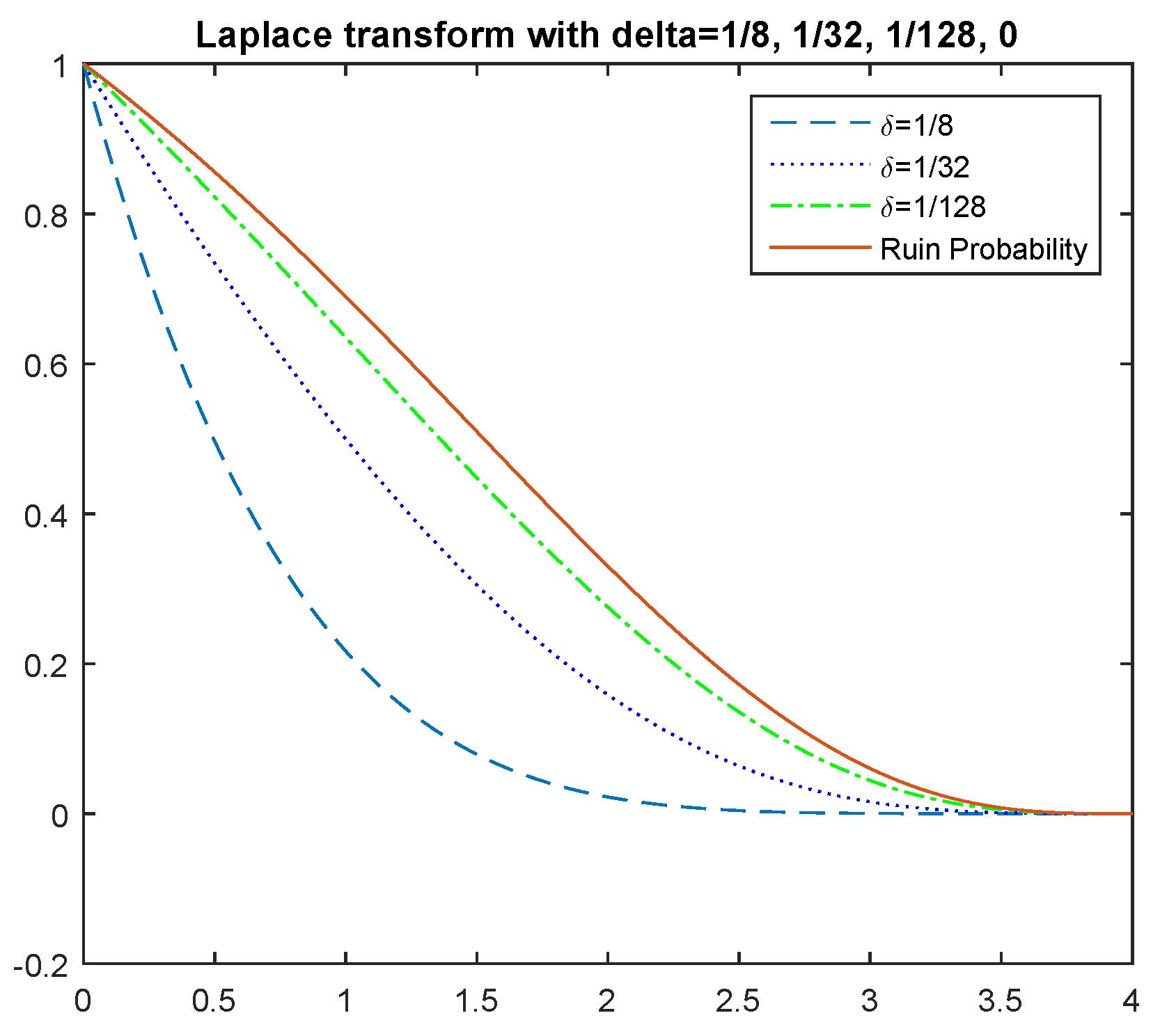
Example 7.

Consider exponentially-distributed gains, where $\overline{F}(x)=e^{-x}$. Let $\frac{c}{a}=b=4$, $\frac{\lambda }{a}=d=3.5$ and $N=100$. Figure 5 shows that the numerical approximation of Φ approaches the ruin probability as $\delta \to 0$. As expected, the Laplace transform of the ruin time is a decreasing function of δ.

6. Conclusions and Future Research

In summary, this paper provides a framework to study numerical approximations of the ruin probability in the dual risk model with a constant interest rate, as well as the Laplace transform of the time of ruin when the gain distribution is arbitrary. Using elementary analysis, the IDE satisfied by the ruin probability can be rewritten as an IE, which in turn can be approximated by a simple linear system.

One possible extension of this work is the numerical approximation for the Gerber–Shiu function. In the classical insurance model, the seminalwork by Gerber and Shiu (1998) builds around the study of the joint distribution of the time of ruin, the surplus immediately before ruin and the deficit at ruin. In the classical dual model, two of the three random variables here are identical. Since ruin is caused by continuous expenses/consumption, the surplus immediately before ruin and the deficit at ruin are both equal to zero. Nevertheless, for the dual risk model, one can study analogs of the Gerber–Shiu function by considering random variables such as the time of the last gain before ruin and its amount (see Yang and Sendova (2014)) or the time of the first gain after ruin and its amount (see Cheung (2012)).