This paper aims to explore the process of deciding whether to adopt technology innovation on a product when facing the uncertainty of environmental changes. During this process, a change in the economic cycle, which is a part of the overall economy, affects consumer purchasing power, while the GDP, which represents future economic growth, is uncertain. The study takes into account the characteristics of product life cycles in the introductory, growth, and maturity stages, and assesses the optimal investment strategies of each stage and project values, as well as the options premiums of the decision-making points.
2.1. Assumptions
The paper assumes sustainable development of high-tech products. According to the product life cycle characteristics, the introduction of technological innovation is divided into three stages (product innovation, manufacturing innovation, and business innovation). It is in the early stage of the three stages to assess whether to invest in innovation cost investment decisions. The investment process must be a sequential investment style. The paper also assumes that consumer purchasing power is highly positively correlated with GDP. According to the historical data of GDP, it is possible to analyze the future GDP that may affect the purchasing power of consumers. At the same time, GDP affects the firm’s revenue, and in time affects the development path of the firm’s investment strategy for product development and innovation technology. Firm’s revenue will also increase when GDP grows. Therefore, the paper is based on the trend of GDP changes in the past, which corresponds to the trend of similar firm’s revenue. The compound binomial options model is used to assume a perfectly efficient market. The change in the price of the target (GDP or revenue) during the duration of the option is used to evaluate the reasonable value of the option. This study split the selection period into T periods, with only two options for each period. One is to increase the fixed range u, and the probability is p, while the other is to fall a fixed range d, and the probability is . The current price of the target (GDP or revenue), after the first period, rises to or falls to . u represents the price increase of the target (), and d the price decrease of the target ().
The study assumes that the changes in GDP affect the purchase and consumption abilities of its citizens, and in turn impact production and revenues. The study analyzed historical data to find possible future GDP occurrences and determine their impact on consumer purchasing power and their further impact on investment strategy development paths concerning their product development in technology innovation. Assume that
is the GDP base stage.
and
are defined as the upward and downward multipliers of the variable GDP in the next period, respectively, and
is satisfied. Let
denote the three stages of technology innovation and
=
I,
II,
III denote the first stage, the second stage, and the third stage respectively. Let
denote the risk-adjusted discounted rate (
Lin 2009;
Lin and Huang 2011), complying with the natural constraints of
. The possible growth path of risk-adjusted probability is
(
Copeland and Antikarov 2001); the decline path of risk-adjusted probability is
(
). This paper shows the GDP change path, the relevant path ratio distribution, and the corresponding GDP nodes of each time frame as shown in
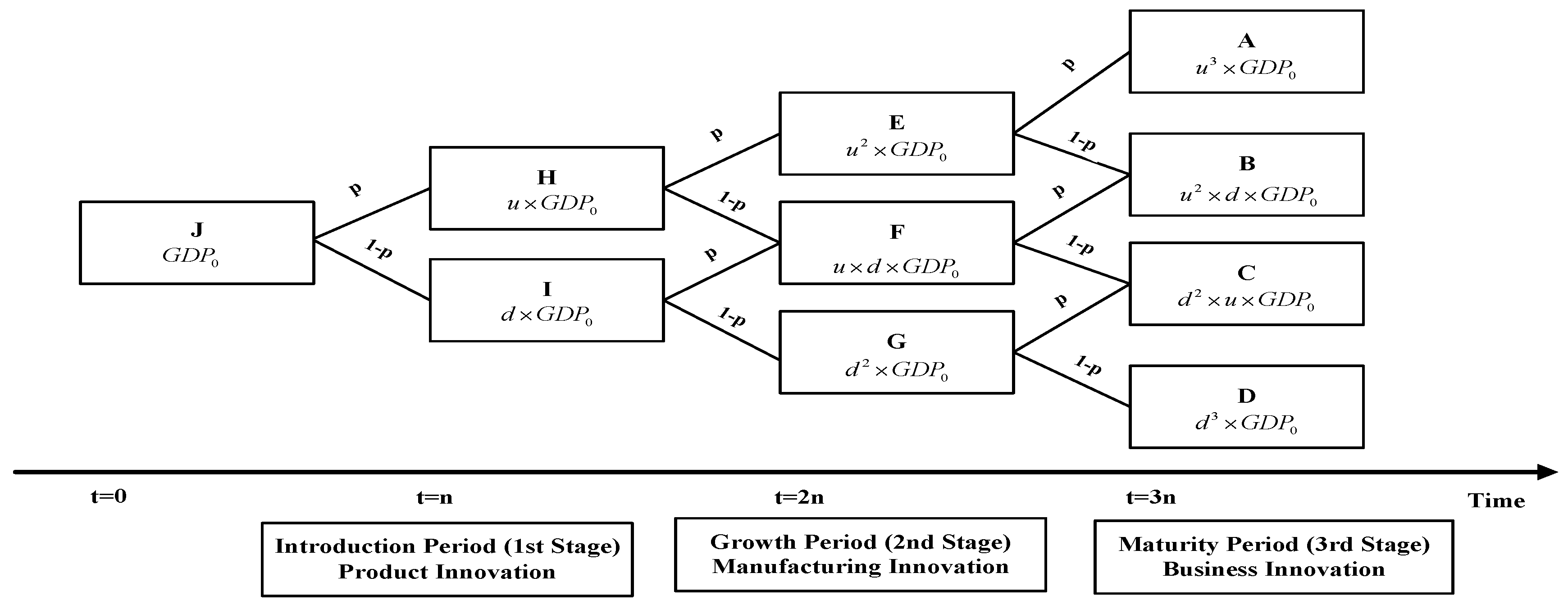
Figure 1 (
Copeland and Antikarov 2001;
Cheng et al. 2011):
In
Figure 1 GDP change path, this study assumes
is the GDP of
i node, where
and
is the GDP of
J node. Then the GDP of
H node is
. In addition, the GDP of
I node is
. Similarly, the GDP of each node is
,
,
,
,
,
, and
, respectively. The expected future revenue of the product corresponding to each node of
Figure 1 is shown in
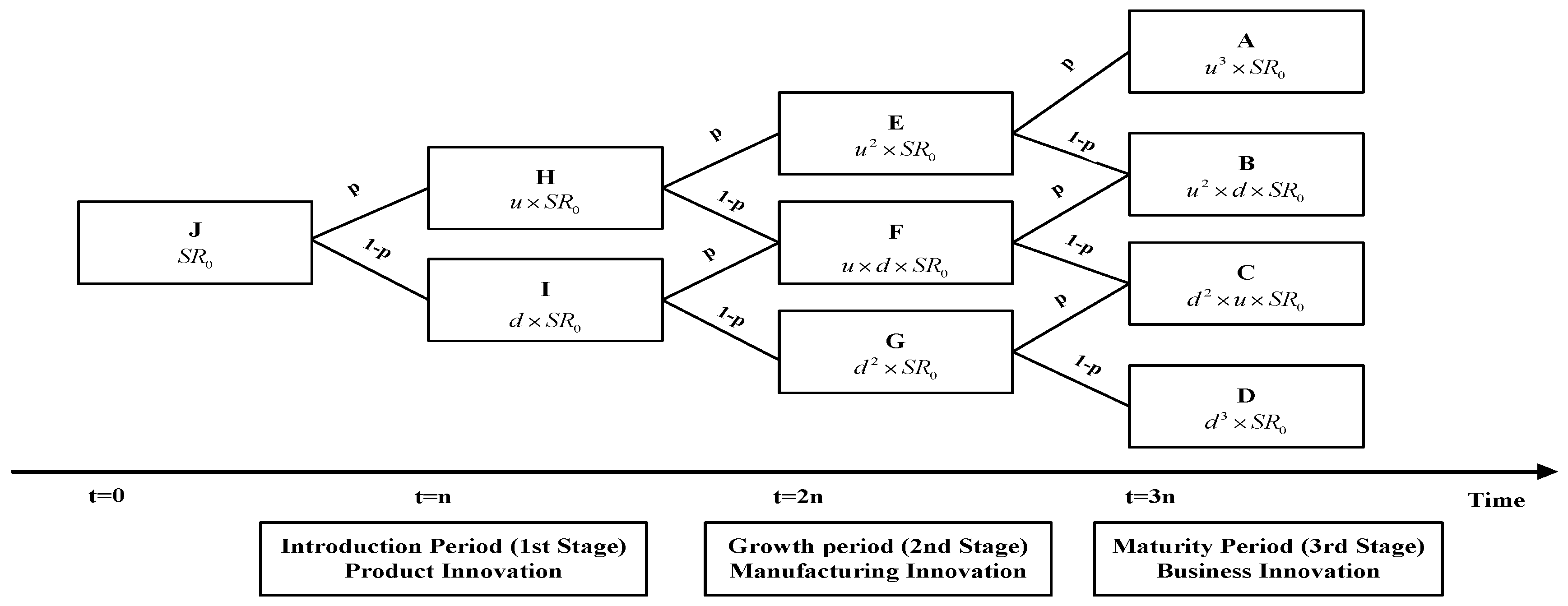
Figure 2 revenue change path (
Copeland and Antikarov 2001;
Cheng et al. 2011):
In
Figure 2 revenue change path, this paper assumes that
is the revenue of
i node, where
and
is the revenue of
J node. Following the GDP variation path in the next step, where the economic growth adjusted-risk probability is
p and the average growth rate of each stage is
, the revenue of
H node is
. In addition, the recession adjusted-risk probability is
and the average recession rate is
; therefore, the revenue of
I node is
. Similarly, the revenue of each node is
,
,
,
,
,
, and
, respectively. That is, there are two possible situations for each node. In one case, the GDP will increase in the case of economic growth, and the corresponding GDP will increase the purchasing power of consumers, and the revenue of firm will also increase. In another case, when the economy is in a recession, the GDP at the node is declining, and the purchasing power of the corresponding consumer is declining, which also results in a decrease in firm revenue.
2.2. Compound Binomial Options
This study utilizes the compound binomial options model (
Copeland and Antikarov 2001;
Cheng et al. 2011) and the three stages of the product life cycle characteristics: introductory, growth, and maturity. For the sustainable operation of the product, each stage requires innovation cost investments: product innovation, manufacturing innovation, and business innovation. According to product life cycle characteristics, the sequence investment program primarily completes the first stage of the introduction period (product innovation) innovation investment, and subsequently moves in the next stage of investment (manufacturing innovation). After completing the second stage of innovation investment, it finally enters the mature period (business innovation) investment strategy.
Due to the long lead time of technology innovation, this paper assumes that the investment strategy in each stage adopts the early assessment investment strategy method. That is, the investment strategy in the E, F, and G nodes of the second stage is to consider whether to invest in business innovation costs, or to abandon the investment project. Similarly, the investment strategy in the H and I nodes of the first stage is to consider whether to invest in manufacturing innovation, while in the stage , the decision is to determine whether product innovation is to be continued or abandoned. Suppose is the innovation cost of the s stage. At the stage, it is to decide whether to invest in the first stage product innovation input cost. At the first stage of the introduction period , it is to decide whether to invest in the second stage of growth and innovation costs. The second stage of the growth phase determines the third stage of business innovation investment strategy.
This study assumes that the investment strategy in each stage adopts the early assessment investment strategy method. Therefore, the consideration factors affecting whether to proceed with the next stage of investment at each revenue node of each stage include the decision point, the expected revenue of the previous stage, and the discounted present value of the revenue of the expected invested innovation cost. That is, at
E node of the 2nd stage, the revenue at the decision point
is included in the added total of the expected revenue of the 1st stage for
n years and the discounted present value of the expected revenue of the 3rd stage after the business innovation cost is invested (
Cheng et al. 2011):
From Equation (1), denotes the revenue of E node decision point, which is the added total of the discounted present value of A and B nodes revenues of the 3rd stage , and the expected revenue . This paper constructs an investment model that incorporates the three stages of innovation strategies of new product development, and uses the early strategic decision method. That is, at the decision point of the 2nd stage, the revenue resulting from the 1st stage strategic options and the present value of the expected revenue of the corresponding expected results of the 3rd stage are considered, which are the results of the adopted strategies at each node of the 2nd stage.
Similarly,
denotes the revenue of
F node decision point as shown in Equation (2) (
Cheng et al. 2011):
Then,
denotes the revenue of
G node decision point as shown in Equation (3) (
Cheng et al. 2011):
Then, at
H node in the 1st stage, the consideration factors, when facing the decision of investing in the manufacturing innovation cost, include the discounted present value of the expected revenues of
E and
F nodes of the 2nd stage
, and the expected revenue
(
Cheng et al. 2011):
Similarly,
denotes the revenue of
I node decision point as shown in Equation (5) (
Cheng et al. 2011):
The revenue of
J node decision point is denoted as
as shown in Equation (6) (
Cheng et al. 2011):
This paper continues to calculate the equity values of nodes E, F, G, H, I, J. Assuming is the equity value of i node of s stage, the rule of the decision is that when the equity value is greater than 0, i.e., , the option is to invest; if the equity value is smaller than 0, i.e., , the option is to abandon the investment or to wait for the next appropriate investment opportunities.
The option of whether to invest in the business innovation cost is at
E node. Its equity value
equals the decision point revenue of the 2nd stage
minus the business innovation cost
invested during the 2nd stage. When the value is greater than 0, the plan of investing in the business innovation cost will be implemented; otherwise, the choice will be to abandon the plan or to wait for the next investment opportunity when the equity value equals 0. The
E node option of whether to invest in the business innovation cost and its equity value are shown in Equation (7):
Additionally, the equity value of
F node
equals the decision point revenue of the 2nd stage
minus the business innovation cost
invested in the 2nd stage. When the value is greater than 0, i.e.,
, the option will be to invest in the business innovation cost; otherwise, the option will be to defer the investment. The
F node option of whether to invest in the business innovation cost and the equity value are shown in Equation (8):
Likewise,
G node equity value
equals the decision point revenue of the 2nd stage
minus the business innovation cost
invested in the 2nd stage. When the value is greater than 0, i.e.,
, the option will be to invest in the business innovation cost; otherwise, the option will be to defer the investment. The
G node option of whether to invest in the business innovation cost and the equity value are shown in Equation (9):
The equity value of
H node
must include the results of the decision point revenue of the 1st stage
minus the invested manufacturing innovation cost
of the 1st stage. It means that when
is greater than 0, it is worth proceeding with the investment. Because the investment decision is correlated to the decision of business innovation investment of the 3rd stage, this consideration must also include the discounted present value of the expected equity return of
E and
F nodes of the 2nd stage
. If the value is greater than 0, it is one of the consideration factors in the manufacturing innovation cost investment decision, that is, when
, investing in the manufacturing innovation cost will be considered. But if
, the option will be to abandon the investment in the manufacturing innovation cost and wait for another opportunity as shown in Equation (10):
Likewise, the equity value of
I node
must include the results of the decision point revenue of the 1st stage
minus the invested manufacturing innovation cost
of the 1st stage. It means that when
is greater than 0, it is worth proceeding with the investment. Because the investment decision is correlated to the decision of business innovation investment of the 3rd stage, this consideration must also include the expected equity values of
F and
G nodes of the 2nd stage
. If the value is greater than 0, it is one of the consideration factors in the manufacturing innovation cost investment decision, that is, when
, investing in the manufacturing innovation cost will be considered. But if
, the option will be to abandon the investment in the manufacturing innovation cost and wait for another opportunity as shown in Equation (11):
The equity value of
J node
includes the results of expected revenue after the product innovation cost is invested
minus the results of whether to invest in the product innovation cost
in stage 0, i.e.,
. In addition, this calculation must also include the expected equity value of
H and
I nodes of the 1st stage
because if the innovation cost is not invested at
J node, neither manufacturing innovation nor business innovation is possible. Therefore, the consideration factor in stage 0 includes the decision to invest the profit in innovation costs. If losses are incurred in stage 0, the equity value of manufacturing innovation of the 1st stage is still one of the consideration factors. That is, when
, investing in the product innovation cost will be considered. But when
, the option is to abandon the investment or to defer to the next investment opportunity as shown in Equation (12):
The equity value
of nodes
E,
F,
G,
H,
I,
J and the equity values of binomial options are shown in
Figure 3:
Figure 3 is the equity values of binomial options. This model employs a compound binomial options approach that is more flexible in strategic thinking than other approach to construct an innovation investment strategy, which is product life cycle specific. Its strategic principle is that when the equity value is greater than 0, i.e.,
, the option is to proceed with the investment; if the value equals 0, i.e.,
, the option is to abandon the investment or to defer to the next appropriate investment opportunity. This model serves as a reference for corporate decision-making in product investment strategies.
Section 3 below uses a firm case study, where One-Time Password’s investment is studied and simulation analysis is performed, providing a basis for managerial reference when considering the product innovation investment.


