An Age Grouping Framework for Multi-Population Mortality Modeling

Abstract

This study extends existing mortality prediction frameworks by incorporating information borrowed from population–gender–age subgroups that exhibit similar mortality patterns. The borrowed information is integrated into classical mortality models to improve the accuracy of future mortality rate forecasts. To capture structural similarities among mortality trajectories, several distance measures are evaluated in combination with four linkage methods, particularly when each subgroup comprises multiple age-specific mortality trajectories. Extensive empirical analyses using data from the Human Mortality Database demonstrate the superior predictive performance of the proposed approach.

1. Introduction

Quantifying the evolution of mortality patterns over time through a well-structured mortality model is a fundamental task for actuaries engaged in life insurance and longevity risk management. Such modeling capabilities enable insurers to manage retirement portfolios more effectively while allowing policymakers to create more accurate forecasts and informed decisions in the design of pension plans and annuity products.

The traditional Lee–Carter model (Lee and Miller 2001; Lee and Carter 1992; Wilmoth 1993) incorporates an age-specific coefficient applied to a common mortality trend, which describes how mortality improves over time across all ages, maintaining consistency within a given dataset. However, this traditional method fails to account for the variation and structural differences in mortality trends between different ages and can eventually lead to unreliable future mortality forecasts.

In order to identify and model both similarities and differences in mortality development patterns across age groups, researchers in this field have introduced solutions based on multiple aspects. On one hand, classical mortality models have been reformulated to address specific age ranges through structural and interpretive modifications. A well-known example is the Cairns–Blake–Dowd (CBD) model (Cairns et al. 2006) and its generalizations (e.g., Cairns et al. 2009), which are particularly valued for their simplicity, interpretability, and predictive accuracy for older age groups. On the other hand, models have been developed to effectively capture distinct mortality dynamics across different ages. Examples include the multi-factor extensions of traditional models that incorporate additional age–period interaction terms (e.g., Booth et al. 2002; Hyndman and Ullah 2007; Renshaw and Haberman 2003) and spline-based approaches in which mortality is modeled non-parametrically using localized basis functions to capture local mortality trends (e.g., Camarda 2012, 2019; Currie et al. 2004; Zhu and Zhou 2023).

When the age range of mortality data is specified, the aforementioned models can be viewed as a tool for borrowing information across different ages. Recent studies have demonstrated that the choice of age range, without adjusting the model structure, can also substantially influence predictive performance. For example, Shang and Haberman (2020) compared models calibrated on full and partial age ranges and found that the selected range affected the forecasting accuracy. Building on this insight, alternative approaches have emerged that enhance mortality model predictions by optimizing the scope of data used for model calibration, rather than constructing entirely new model structures. This strategy aims to leverage the most relevant age information to improve the predictive accuracy. For instance, Wang et al. (2021) incorporated information from neighboring ages to strengthen forecasts, while Tsai and Cheng (2021) applied statistical clustering to filter mortality data and extract representative patterns. Similarly, Meng et al. (2025) proposed an individual age-specific band selection framework that borrows information from adjacent ages to train prediction models for each age, achieving notable improvements in accuracy.

This paper builds on the idea of filtering data and extends the individual age-specific framework from (Meng et al. 2025) to a more general age grouping-based mortality prediction framework. Unlike existing approaches that model each age separately, the proposed framework allows ages with similar mortality development patterns due to being in the same life stage to be grouped together, reflecting the belief that human mortality evolves differently across various stages of life. Meanwhile, the framework further leverages the well-established benefits of multi-population modeling to improve the predictive accuracy (e.g., Diao et al. 2021, 2023; Enchev et al. 2017; Li and Lee 2005; Russolillo et al. 2011; Shang and Hyndman 2017) through a fully data-driven procedure that simultaneously borrows information across populations, genders, and age groups with similar mortality trends to the target.

This paper contributes to this strand of research in the following ways. First, it extends the distance-based approach of the individual age-specific framework in (Meng et al. 2025) by allowing flexible choices of both distance measures and linkage functions and by incorporating an ensemble-based averaging procedure to enhance the stability and accuracy of the resulting predictions. Second, the proposed framework offers a direct and computationally efficient solution that closely aligns with real-world actuarial practice, in which mortality is typically modeled and projected at the age group level rather than at each individual age for insurance applications. The life stage-based grouping procedure limits the number of prediction targets, ensures relatively stable mortality patterns within each group, reduces the roughness and noise inherent in highly granular age-specific models, and avoids the computational and methodological burden of extensive data-driven features through engineered group selection. Extensive empirical comparisons using the Human Mortality Database confirm the effectiveness of the proposed method in improving predictive performance.

The remainder of this manuscript is structured as follows. Section 2 provides a detailed description of the proposed age grouping-based mortality prediction framework, along with the data mining procedure that is involved in the framework. Section 3 presents the empirical results, comparing the proposed method with traditional benchmark models based on an analysis of the Human Mortality Database to assess the overall performance. Finally, Section 4 summarizes the key findings and concludes the paper.

2. Methodology

Traditional single-factor mortality models, such as the Lee–Carter model, apply age-specific coefficients to a common mortality trend that captures how mortality improves over time across all ages. However, these models do not adequately account for variations and structural differences in mortality trends across ages, which can lead to unreliable long-term forecasts. Although introducing additional variables or model components can address these age-specific variations, achieving the appropriate balance between model complexity and interpretability remains challenging, as overly complex models are more susceptible to misspecification and may potentially result in reduced predictive performance. A newly emerging alternative is to incorporate a data filtering process that controls which data are included in the model calibration step. The idea is to retain only the data that share structurally similar mortality trajectories with the target, while filtering out those with different patterns. This approach can help to ensure the validity of the model, bringing potential improvements in prediction accuracy to our mortality-predicting target without the need to increase the complexity of the underlying mortality model.

Building on this idea, we extend the distance-based individual age-specific framework of Meng et al. (2025) to a more comprehensive age grouping framework. This new generation of methods integrates the data filtering process within a multi-population setting, grouping and selecting data across populations, genders, and ages. Our fully data-driven procedures robustly quantify the structural similarities in mortality trajectories among population–gender–age groups, enabling an optimal balance between incorporating beneficial information and filtering out less relevant data to enhance the mortality prediction accuracy of the predicting target.

2.1. Individual Age Mortality Modeling Frameworks

Before introducing our proposed method, we first outline the distance-based individual age-specific framework in (Meng et al. 2025). Let $\mathcal{X}:=\{x_L,x_{L+1},\dots ,x_U\},(x_L\ge 0,x_U\le 100)$ and $\mathcal{T}=\{t_L,t_{L+1},\dots ,t_U\}$ denote the age and time ranges of the available mortality data. The individual age-specific framework decomposes the overall mortality prediction task into separate prediction tasks for each age $x_0\in \mathcal{X}$. For each target age $x_0$, a data-driven procedure selects an age-specific set ${\mathcal{A}}_{x_0}^{*}$ that contains both the target age $x_0$ and a set of reference ages to be used in the subsequent mortality modeling step.

For scenarios in which the individual age-specific framework is implemented in a single-population scenario where mortality data from different ages of the same population are filtered to enhance the prediction accuracy, Meng et al. (2025) outlined a method to define ${\mathcal{A}}_{x_0}^{*}$ for the target age $x_0$ as a symmetric or asymmetric age band that includes both the target age $x_0$ and some neighboring ages, with the rationale that adjacent ages typically exhibit greater similarity in mortality development patterns compared to ages that are further apart. When the individual age-specific framework is implemented in a multi-population scenario where information from other populations can be incorporated simultaneously, the notion of a “neighborhood” for a target age is generalized beyond the natural age ordering. Instead, the neighborhood is defined as the set of ages across all available populations that exhibit the greatest similarity to the target age, as determined by some proposed distance measures.

The individual age-specific framework can be embedded with many classic mortality models. For example, when the Lee–Carter model (Lee and Carter 1992) is embedded, we conduct the estimation regarding the following formulation and data range:

$$logm(x,t)=a_x+b_x{k}_t+{ϵ}_{x,t},x\in {\mathcal{A}}_{x_0}^{*},t\in \mathcal{T},$$

(1)

where $m(x,t)$ denotes the central death rate, also known as the age-specific death rate (ASDR), for  the age $x\in {\mathcal{A}}_{x_0}^{*}$ and year $t\in \mathcal{T}$ of a population. The model has normalization constraints ${\sum }_x{b}_x=1$ and ${\sum }_t{k}_t=0$. ${ϵ}_{x,t}$s are independent and identical residuals with zero mean and finite age-specific variance ${\sigma }_x^2$. The estimation of the parameters in the Lee–Carter model follows the standard non-likelihood-based method using singular value decomposition (SVD). The static age function $a_x$ is estimated as the average of the logarithmic ASDRs over the modeling time period,

$${\widehat{a}}_x={\displaystyle \frac{1}{t_U-t_L+1}}\sum _{t=t_L}^{t_U}log{m}_{x,t},$$

(2)

and $b_x$ and $k_t$ are, respectively, identified as the first left and first right singular vectors of the matrix $log{m}_{x,t}-{\widehat{a}}_x$. The mortality prediction for the target age $x_0$ is then obtained by extrapolating the calibrated mortality model by assuming an appropriate time series model, e.g., a random walk with drift (RWD), for the mortality index $k_t$.

2.2. Age Grouping Framework

The primary motivation for extending the individual age-based framework to an age grouping framework is to overcome several limitations of the original approach. Although age-specific mortality rate series exhibit distinct patterns across ages, many single-age series lack robustness due to limited exposure or inherently volatile dynamics. Moreover, from a practical implementation perspective, actuaries typically model mortality at the age group level, such as infants, working-age adults, or retirees, corresponding to broader life stages. Grouping adjacent ages provides a natural means of improving the statistical stability by increasing exposure within each group, while still preserving meaningful heterogeneity across groups. Since mortality dynamics differ systematically across these stages, grouping by life stage is both intuitive and well aligned with real-world actuarial practice.

In contrast to the individual age-based framework, which relies exclusively on a variance-based distance metric, the proposed framework provides a more comprehensive and flexible approach in several respects. First, it introduces an age grouping procedure based on life stages, consistent with real-world actuarial practice, in which mortality is commonly analyzed at the age group level; this grouping enhances the estimation robustness and reduces the computational burden. Second, the framework allows for a richer class of distance measures, overcoming the limitations of relying solely on variance-based metrics. Third, it defines group-level similarity metrics for multi-dimensional time series through alternative linkage functions, thereby clarifying how overall group-to-group similarity is constructed, rather than restricting comparisons to age-to-age relationships. Finally, the framework incorporates an ensemble-based averaging strategy to aggregate predictions, further improving its robustness.

In the remainder of this subsection, we provide a detailed introduction to each of the aforementioned components of the proposed framework.

2.2.1. Age Grouping Process

Mortality rates vary considerably across individual ages, yet adjacent ages within the same stage of life generally display similar trends. For instance, a 15 year old’s mortality pattern is much closer to that of a 20 year old than to that of a 95 year old. This pattern is evident in Figure 1, which shows age-specific logarithmic mortality rates for Canadian females over time. Our age grouping procedure builds on this observation by predefining age groups under the assumption that ages within the same life stage share common mortality development patterns, while ages from different life stages will exhibit different behaviors. Accordingly, we define six age groups: the infant group (Age 0), the child group (Ages 1–10), the teen group (Ages 11–20), the adult group (Ages 21–65), the retiree group (Ages 66–85), and the old group (Ages 86–100). Although there is no universally accepted rule for the exact age thresholds that distinguish these groups, these choices are consistent with both conventional age decompositions used in the past mortality literature and common practice in real-world settings for distinguishing life stages. Some examples of past work that adopts similar age thresholds can be found in (Fu et al. 2025; Giordano et al. 2019; Meng et al. 2025; Shang and Haberman 2020; Tsai and Cheng 2021).

We therefore treat each age group $B_i$ within each population $p_j$ and gender $g_k$ as a distinct predicting target, denoted by $(B_i,p_j,g_k)$. This decomposition yields $6\times 24\times 2=288$ target datasets. Extending our notation, let ${\mathcal{A}}_{B_i,p_j,g_k}^{*}$ represent the dataset selected for the mortality model corresponding to the target $(B_i,p_j,g_k)$ (age group $B_i$, population $p_j$, and gender $g_k$) to optimally enhance the predicting performance of the target. The mortality sequences from both the predicting target $(B_i,p_j,g_k)$ and potentially additional reference sequences from different populations, genders, or age groups are stacked by row to form a new combined mortality matrix. A general Lee–Carter-type model is embedded to model the mortality dynamics of the selected dataset ${\mathcal{A}}_{B_i,p_j,g_k}^{*}$ based on the combined matrix and can be written as follows:

$$log{m}_{x,t}=a_x+\sum _{s=1}^S{b}_x^{\left(s\right)}{k}_t^{\left(s\right)}+{ϵ}_{x,t},x\in {\mathcal{A}}_{B_i,p_j,g_k}^{*},t\in \mathcal{T}.$$

(3)

where $b_x^{\left(s\right)}$ and $k_t^{\left(s\right)}$ represent the s-th order of the age/period effects that are shared among all members in the selected dataset ${\mathcal{A}}_{B_i,p_j,g_k}^{*}$. Once the dataset is determined, the static age function $a_x$ is still estimated as the average of the logarithmic ASDRs over the modeling time period, and $b_x^{\left(s\right)}$ and $k_t^{\left(s\right)}$ are, respectively, identified as the first s left and right singular vectors of the matrix $log{m}_{x,t}-{\widehat{a}}_x$. Then, the mortality prediction for the target $(B_i,p_j,g_k)$ is obtained using the standard extrapolation procedure, as previously described.

2.2.2. Choice of $A_{B_i,p_j,g_k}^{*}$

In this subsection, we introduce our proposed, fully data-driven procedure that determines the $A_{B_i,p_j,g_k}^{*}$ for each of our targets $(B_i,p_j,g_k)$ from all available datasets to improve the predicting accuracy of the target. Following the principles of the distance-based method in (Meng et al. 2025), the selected dataset $A_{B_i,p_j,g_k}^{*}$ would leverage information from other population–gender–age groups that exhibit a large amount of similarity in mortality development patterns, as measured by a defined similarity measure, through the following steps.

• Define a similarity measure between two population–gender–age groups, $G_T$ and $G_R$ (T for the target and R for the reference), using a function $f_{G_T;G_R}$, where smaller values indicate greater similarity in their mortality development patterns over time.
• For a target population–gender–age group $G_T=(B_i,p_j,g_k)$, compute $f_{G_T;G_R}$ for every potential reference group $G_R$ in the reference pool and sort the results in ascending order to rank the structural similarity of each reference group to $G_T$.
• Predefine a constant K, representing the maximum number of reference groups allowed to contribute information.
• Among these K nearest “neighbors”, select only the top k groups to borrow information from, following the well-known K-nearest neighbors (KNN) algorithm (Fix and Hodges 1989). The parameter k can take possible values within $\{0,1,\cdots ,K\}$ and determines the size of the “neighborhood”, reflecting the extent of information borrowing.
• Selecting the optimal set of neighboring groups reduces to choosing the best neighborhood size k within a prespecified range $\{0,1,2,\cdots ,K\}$ using a standard validation procedure. If the selected group size is $k=0$, no information is borrowed from neighboring groups, and the set ${\mathcal{A}}_{B_i,p_j,g_k}^{*}$ contains only the prediction target $(B_i,p_j,g_k)$ itself.

Quantifying the structural similarity between the mortality development patterns of any two population–gender–age groups using $f_{G_T;G_R}$ requires the following two components: a pairwise distance measure that evaluates the similarity between individual age-specific mortality rate series and a linkage function that aggregates these pairwise distances into an overall similarity score for the two groups. We outline the candidate methods considered for both components in the following.

2.2.3. Distance Measure

• Variance-Based Distance:
  This function follows the same design used in (Meng et al. 2025) to ignore differences arising from varying mortality levels, allowing two parallel mortality trajectories at different levels to be treated as exhibiting highly similar developmental trends. Assuming two mortality trajectory sequences $\mathbf{x}\left(t\right)$ and $\mathbf{y}\left(t\right)$, the proposed distance measure is defined as follows.

  (1)

  Define a difference sequence as

  $${\mathrm{diff}}_{x;y}\left(t\right)=\mathbf{x}\left(t\right)-\mathbf{y}\left(t\right),t\in \mathcal{T},$$

  where the difference sequence represents the difference between the mortality sequences $\mathbf{x}\left(t\right)$ and $\mathbf{y}\left(t\right)$.

  (2)

  Define the distance measure by the variance of the difference sequence, i.e.,

  $$D_{\mathrm{var}}(\mathbf{x};\mathbf{y})=\mathrm{Var}\left({\mathrm{diff}}_{x;y}\left(t\right)\right).$$

  A lower value indicates greater resemblance among the two mortality sequences. $D_{\mathrm{var}}(\mathbf{x};\mathbf{y})=0$ for two parallel sequences that have a constant difference over time.
• Dynamic Time Warping-Based Distance:
  Dynamic time warping (DTW) (Berndt and Clifford 1994) is a widely used technique for measuring similarity between two time series by allowing non-linear stretching and compression along the time axis. It offers two key advantages: first, it does not require time series of equal length, making it suitable for mortality sequences that are not temporally aligned; second, unlike the variance-based distance that relies on pointwise comparisons and assumes perfect alignment, the DTW-based distance is more robust to temporal shifts and local delays, providing a more reliable similarity measure when similar patterns occur at slightly different times. The warped time concept relies on the mathematical idea that time does not need to be treated as a fixed, linear calendar scale; it can be transformed to better align with structural dynamics. This is consistent with the operational time used in Reliability Theory from the 1950s and introduced into the actuarial literature by Bühlmann (1967).
  The following summarizes the general procedure used to obtain the DTW-based distance between two given sequences $\mathbf{x}\left(t\right)$ and $\mathbf{y}\left(t\right)$ of lengths n and m. In brief, the DTW-based distance seeks an alignment that minimizes the cumulative distance under temporal distortions.

  (1)

  Define a local distance measure, denoted as $d(x_i,y_j)$. Using this measure, an $n\times m$ cost matrix is constructed,

  $$D(i,j)=d(x_i,y_j),1\le i\le n,1\le j\le m.$$

  (2)

  Compute the minimal global alignment via dynamic programming, using the cumulative cost matrix

  $$C(i,j)=D(i,j)+min\left\{C\right(i-1,j),C(i,j-1),C(i-1,j-1\left)\right\},$$

  with $C(1,1)=D(1,1)$ and boundary values set to $+\infty$ to enforce valid paths. These choices correspond to vertical, horizontal, or diagonal steps, allowing one point in one series to align with one or more points in the other.

  (3)

  An admissible alignment is represented by a warping path that specifies which elements of $\mathbf{x}\left(t\right)$ are matched with which elements of $\mathbf{y}\left(t\right)$,

  $$W=\left((i_1,j_1),\dots ,(i_L,j_L)\right),$$

  which must start at $(1,1)$, end at $(n,m)$, be monotone, and move only in steps $(1,0)$, $(0,1)$, or $(1,1)$, ensuring continuity and temporal order.

  (4)

  The DTW-based distance is defined as the minimal cumulative cost of this optimal path:

  $$D_{\mathrm{DTW}}(\mathbf{x},\mathbf{y})=C(n,m).$$

  Based on different specifications regarding the local distance, we specify the DTW-based distance functions used in this project as follows.
  • Dynamic Time Warping (DTW) Distance:
    The local distance measure is defined as the squared Euclidean distance, i.e.,

    $$d(x_i,y_j)={(x_i-y_j)}^2.$$
  • Derivative Dynamic Time Warping (DDTW) Distance:
    Derivative dynamic time warping (DDTW) (Keogh and Pazzani 2001) measures the similarity between time series by aligning estimated local derivatives rather than raw values, thereby emphasizing shape over magnitude and treating sequences with more similar local derivatives as closer to one another. Given two sequences $\mathbf{x}\left(t\right)$ and $\mathbf{y}\left(t\right)$, we first compute discrete derivative (slope) estimates for each series,

    $$d_x\left(i\right)=\left\{\begin{array}{cc}{d}_x\left(2\right),\hfill & i=1,\hfill \\ {\displaystyle \frac{(x_i-x_{i-1})+\frac{(x_{i+1}-x_{i-1})}{2}}{2}},\hfill & 2\le i\le n-1,\hfill \\ d_x(n-1),\hfill & i=n,\hfill \end{array}\right.$$

    and similarly for $\mathbf{y}\left(t\right)$. The local distance between time points is then defined as the squared difference of derivatives:

    $$d(x_i,y_j)={\left(d_x\left(i\right)-d_y\left(j\right)\right)}^2,1\le i\le n,1\le j\le m.$$
  • Shape Dynamic Time Warping (ShapeDTW) Distance:
    Shape dynamic time warping (ShapeDTW) (Zhao and Itti 2018) is designed to produce locally meaningful alignments. Rather than warping the raw time series values, ShapeDTW aligns sequences of local shape descriptors extracted from the series, enhancing the robustness to noise and shifts in the original sequences. ShapeDTW consists of two main steps: encoding local structures using shape descriptors and aligning the resulting descriptor sequences via DTW. Specifically, for each time point, a subsequence of window size h is extracted to form a shape descriptor, transforming the original time series into a descriptor sequence of equal length. DTW is then applied to align the descriptor sequences, and the resulting warping path is transferred back to the original time series. Given two sequences $\mathbf{x}\left(t\right)$ and $\mathbf{y}\left(t\right)$, we first extract the local shape descriptor

    $${\mathbf{s}}_i=f\left(x_{i-\lfloor h/2\rfloor },\dots ,x_{i+\lfloor h/2\rfloor }\right),{\mathbf{t}}_j=f\left(y_{j-\lfloor h/2\rfloor },\dots ,y_{j+\lfloor h/2\rfloor }\right),$$

    for $i\in \{\lfloor h/2\rfloor +1,\lfloor h/2\rfloor +2,\cdots ,n-\lfloor h/2\rfloor \}$ and $j\in \{\lfloor h/2\rfloor +1,\lfloor h/2\rfloor +2,\cdots ,m-\lfloor h/2\rfloor \}$. $f(·)$ may represent the raw subsequence in our subsequent analysis, but it can also be chosen as a derivative-based descriptor or another feature mapping. This produces descriptor sequences $\mathbf{S}=({\mathbf{s}}_{\lfloor h/2\rfloor +1},\dots ,{\mathbf{s}}_{n-\lfloor h/2\rfloor })$ and $\mathbf{T}=({\mathbf{t}}_{\lfloor h/2\rfloor +1},\dots ,{\mathbf{t}}_{m-\lfloor h/2\rfloor })$.
    The local distance between descriptors is defined as

    $$D(i,j)=\parallel {\mathbf{s}}_i-{\mathbf{t}}_j{\parallel }_2^2,\lfloor h/2\rfloor +1\le i\le n-\lfloor h/2\rfloor ,\lfloor h/2\rfloor +1\le j\le m-\lfloor h/2\rfloor .$$

Figure 2 illustrates the alignment patterns of two representative logarithmic mortality rate sequences under different distance measures. The variance-based distance enforces strict one-to-one alignment at each time point due to its reliance on pointwise differences. In contrast, DTW-based methods relax this constraint by searching for a minimum-cost warping path that allows many-to-one alignments and accommodates sequences of unequal length. However, as shown in the second subfigure of Figure 2, applying DTW directly to raw logarithmic mortality rates can yield unintuitive alignments, motivating further refinements such as standardization, DDTW, and ShapeDTW, each of which produces distinct alignments and corresponding distance measures.

2.2.4. Linkage Function

To assess the similarity between population–gender–age groups that contain multi-dimensional time series with different dimensionalities, we employ a linkage function, which aggregates individual age-to-age distances into a meaningful group-to-group distance. Linkage functions are widely used in clustering methods, where different linkage choices can lead to varying similarity rankings among population–gender–age groups. Among the linkage functions considered in this project, we recommend the following.

• Complete Linkage: Calculate the pairwise distance measuring function between all members (individual age) from both population–gender–age groups. Then, choose the maximum value as the similarity measure between the population–gender–age groups, i.e.,

  $$f_{G_T;G_R}=\max \left(D(\mathbf{x},\mathbf{y})\right),\mathbf{x}\left(t\right)\in G_T;\mathbf{y}\left(t\right)\in G_R.$$

  (4)
• Average Linkage: Calculate the pairwise distance measuring function between all members (individual age) from both population–gender–age groups. Then, choose the average value as the similarity measure between the population–gender–age groups, i.e.,

  $$f_{G_T;G_R}=\mathrm{mean}\left(D(\mathbf{x},\mathbf{y})\right),\mathbf{x}\left(t\right)\in G_T;\mathbf{y}\left(t\right)\in G_R.$$

  (5)

Figure 3 illustrates the linkage functions used in our analysis, including centroid linkage, which measures similarity as the distance between the centroid sequences of two population–gender–age groups, and single linkage, which defines similarity as the minimum pairwise distance between the groups. Complete and average linkages are recommended due to their underlying assumptions. Complete linkage emphasizes global cohesion by requiring all pairwise distances to be small, while average linkage balances local and global similarities by averaging distances across pairs. In contrast, single linkage is sensitive to noise and outliers because it relies on the closest pair, and centroid linkage focuses on overall mean patterns, with limited attention to within-group variability.

2.2.5. Ensemble-Based Procedure

Having proposed a rich pool of distance measures to address the limitations of relying on a single metric, and having defined the group-to-group similarity from age-to-age similarity using different linkage functions, the next step is to leverage the predictive outputs from multiple base learners. Traditional approaches focus on selecting one “optimal” combination of the distance measure and the linkage function while discarding all other candidates. However, this strategy does not guarantee optimality, as it is vulnerable to model misspecification and may overlook valuable information captured by the omitted models.

As an alternative, we adopt an ensemble-based approach that combines predictions from multiple base learners to produce a final prediction that is more stable and robust than when applying single models. This methodology has been increasingly incorporated into mortality prediction frameworks (see, e.g., Chang and Shi 2023; Diao et al. 2023; Kessy et al. 2021; Li 2023; Li et al. 2025).

For a given population–gender–age target, we fit a base learner predictive model that specifies the underlying mortality model, the distance measure, and the linkage function according to the previously introduced modeling procedure. This procedure automatically selects reference mortality data and generates mortality predictions through joint modeling. We then denote the mortality prediction of this target $G_T=(B_i,p_j,g_k)$ at calendar year t based on the sth base learner as ${\eta }^{\left(s\right)}(G_T,t),s=1,\dots ,S$. Moreover, the final ensemble prediction takes the general form of

$$\widehat{\eta }(G_T,t)=\sum _{s=1}^S{w}_s{\eta }^{\left(s\right)}(G_T,t),$$

(6)

where $w_s$ is the weight assigned to the sth base learner. In this project, we adopt a simple averaging approach where $w_s={\displaystyle \frac{1}{S}}$. We choose this unweighted averaging method over any “filter-then-average” strategy because the simple average is widely documented to outperform selection-based approaches and is supported by strong statistical rationale. Averaging across all learners substantially reduces variance and leads to more robust performance, even when some models are individually weaker. In contrast, a “filter-then-average” procedure does not necessarily achieve the lowest test SSE due to the existence of estimation errors and model misspecification risks in real applications.

3. Empirical Study

3.1. Dataset and Models

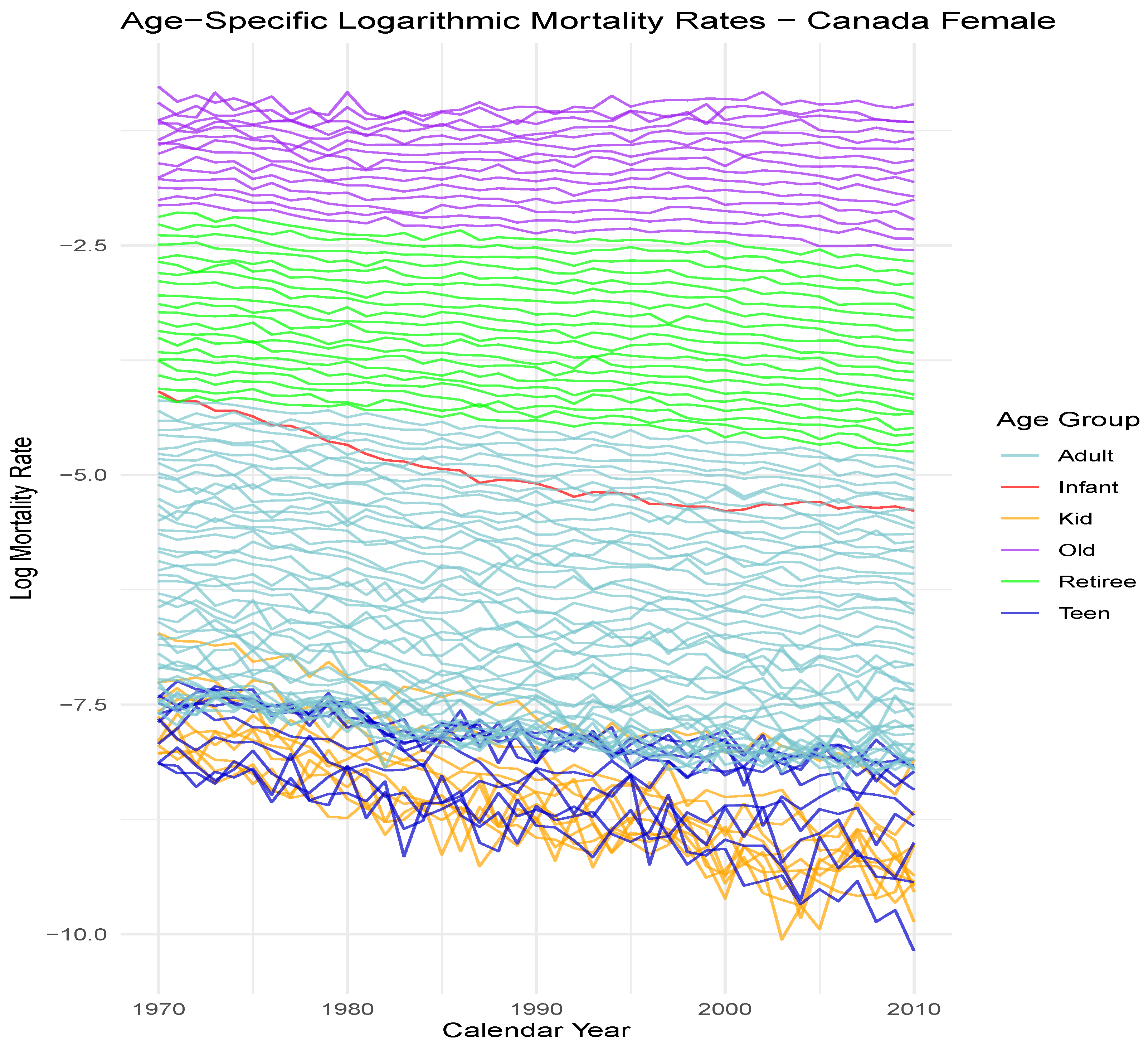
In this section, we empirically evaluate the performance of the proposed framework using data from the Human Mortality Database (HMD) and conduct a comprehensive comparison with a classic mortality model. The HMD is widely regarded as the world’s leading scientific resource for mortality data, providing detailed, consistent, and reliable information for longevity research. Its high-quality data ensure that the models trained are grounded in realistic and actuarially meaningful observations. We obtain mortality data from 24 countries or populations, as listed in

Table 1. The 24 populations from the HMD.

Target Population
Australia	Netherlands
Austria	New Zealand
Japan	Norway
Belgium	Poland
Scotland	Portugal
Canada	U.S.A.
Czech Republic	Slovakia
Denmark	Spain
Finland	Sweden
France	Switzerland
Hungary	Taiwan
Italy	England and Wales

. The dataset includes male and female mortality rates for ages 0 through 100, spanning a 50-year period from 1970 to 2019. Following established practice in longevity research (e.g., Lee and Miller 2001; Tuljapurkar et al. 2000), we select a period of sufficient length that avoids apparent structural breaks. The chosen time frame excludes potential structural changes prior to 1970 and omits the COVID-19 pandemic years, whose long-term mortality effects are still under active investigation.

The dataset is split into a training set spanning from 1970 to 2010 and a test set covering from 2011 to 2019. Each prediction model is fitted using the training period and then extrapolated to the test period to generate mortality forecasts.

The models that we compare with our proposed models include the following.

• LCAllAges: This is the traditional Lee–Carter model in which data from all available ages from one specific gender of one specific population are modeled separately in one model.
• LCOneAge: This method only uses data from the target dataset $G_T=(B_i,p_j,g_k)$ to be trained in the underlying Lee–Carter model, without considering incorporating any other datasets.

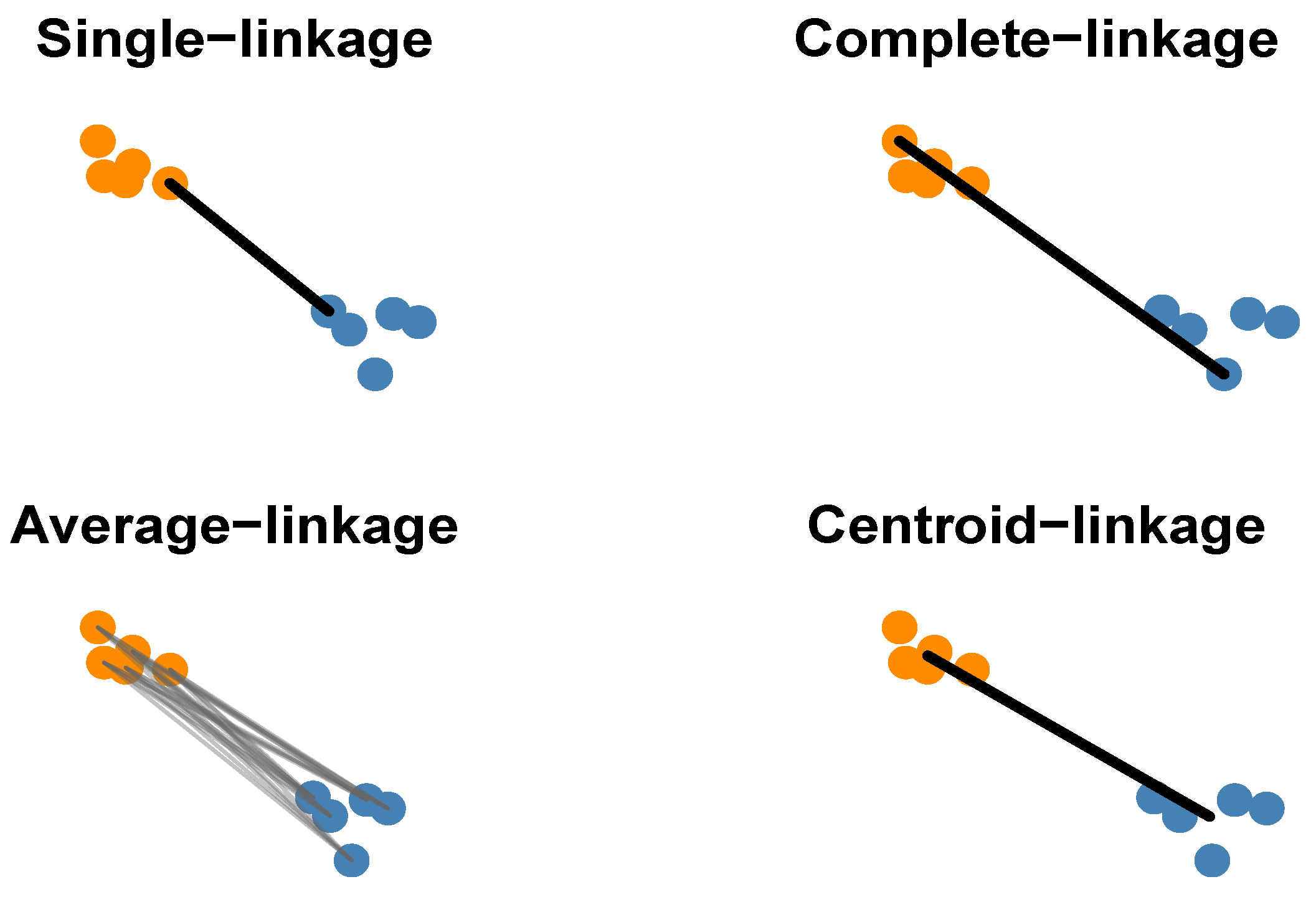
While we continue to use the Lee–Carter model as the underlying mortality model, the methods within our proposed age grouping framework are distinguished by their respective choices of four linkage functions (centroid linkage, single linkage, complete linkage, and average linkage) and the following distance functions.

• VarianceDiff: The distance between two age-specific logarithmic mortality rate sequences is defined as the variance in their difference sequences.
• DTW: The DTW distance computed directly from the original age-specific logarithmic mortality rate sequences. The implementation of the DTW procedure is based on the R package dtw (Giorgino 2009).
• Standardized DTW (SDTW): The DTW distance computed from standardized age-specific logarithmic mortality rate sequences (scaled to zero mean and unit standard deviation).
• DDTW: The DDTW distance computed from standardized age-specific logarithmic mortality rate sequences.
• ShapeDTW: The ShapeDTW distance with window size $h=7$, computed from standardized age-specific logarithmic mortality rate sequences.

This will yield the following $4\times 5=20$ proposed age grouping base model for each predicting target. A validation step is required for each proposed age grouping base model to determine the optimal choice of k from $\{1,2,3,\cdots ,K=20\}$ for each predicting target, with the training set further decomposed into a modeling period from 1970 to 2001 and a validation period from 2002 to 2010 to support this selection. Setting the maximum value at $K=20$ allows a balance between data sufficiency and diminishing marginal gains. Smaller values of K do not provide adequate information for population–gender–age targets with sparse or highly volatile observations—particularly at older ages—whereas larger values of K tend to introduce additional noise into the training process, thereby weakening the predictive performance. The final simple average step will take the average of the predictive results from base models that use the same linkage function but different distance measuring functions by assigning equal weights. All resulting methods are demonstrated in

Table 2. Proposed age grouping methods in this numerical study.

LC-VarianceDiff-Centroid	LC-VarianceDiff-Single	LC-VarianceDiff-Complete	LC-VarianceDiff-Average
LC-DTW-Centroid	LC-DTW-Single	LC-DTW-Complete	LC-DTW-Average
LC-SDTW-Centroid	LC-SDTW-Single	LC-SDTW-Complete	LC-SDTW-Average
LC-DDTW-Centroid	LC-DDTW-Single	LC-DDTW-Complete	LC-DDTW-Average
LC-ShapeDTW-Centroid	LC-ShapeDTW-Single	LC-ShapeDTW-Complete	LC-ShapeDTW-Average
LC-SimAvg-Centroid	LC-SimAvg-Single	LC-SimAvg-Complete	LC-SimAvg-Average

.

3.2. Predicting Performance

The performance measure that we use to assess the predictive accuracy of a model is the total sum of squared errors (SSE), which represents the model’s performance on the test dataset. This method of measurement for mortality models is regarded as one of the standard paradigms for evaluating overall model performance and is widely used in the community (e.g., Diao et al. 2021, 2023; Tsai and Cheng 2021, etc.).

For a given predicting target $G_T=(B_i,p_j,g_k)$, let $e\left(t\right)$ denote its age-aggregated test SSE, computed as

$$e\left(t\right)=\sum _{x\in G_T}{\left[logm(x,t)-log\widehat{m}(x,t)\right]}^2,t\in \mathit{Test}\mathit{Period}$$

(7)

where $m(x,t)$ represents the observed age-specific mortality rate in the test period and $\widehat{m}(x,t)$ is the corresponding model prediction. The overall SSE for any model is then calculated as ${\sum }_{t\in \mathit{Test}\mathit{Period}}e\left(t\right)$, which measures the total prediction error for all ages x in the predicting target $G_T$. To provide a comprehensive assessment of each model’s performance, we compute the overall test SSE across all target population–gender–age groups $G_T$ and report the first quartile, median, sample mean, and third quartile for these SSE values. A smaller aggregate SSE indicates stronger predictive performance. The results are presented in

Table 3. Summary statistics of test SSEs for prediction performance of Complete Linkage age-grouping methods compared to baseline models for genders and all age groups combined. Numbers in parentheses record the rank of predicting performance for each reported summary statistic of test SSEs for genders and all age groups combined. Lower ranks indicate better performance.

	1st Quartile	Median	Mean	3rd Quartile	Average Rank
Female Population
LCAllAges	0.7649 (8)	3.4817 (8)	10.1457 (8)	17.7492 (6)	(7.75)
LCOneAge	0.4747 (4)	2.8163 (6)	10.1414 (7)	18.9084 (8)	(6.25)
LC-VarianceDiff-Complete	0.5128 (7)	2.8721 (7)	9.5625 (3)	17.7030 (4)	(5.25)
LC-DTW-Complete	0.4766 (5)	2.7232 (4)	10.0752 (6)	18.2780 (7)	(5.50)
LC-SDTW-Complete	0.46606 (3)	2.7854 (5)	9.5888 (4)	17.7484 (5)	(4.25)
LC-DDTW-Complete	0.4898 (6)	2.7148 (2)	9.6456 (5)	17.4455 (1)	(3.50)
LC-ShapeDTW-Complete	0.4455 (1)	2.7174 (3)	9.5413 (1)	17.5548 (2)	(1.75)
LC-SimAvg-Complete	0.4601 (2)	2.7116 (1)	9.5623 (2)	17.5600 (3)	(2.00)
Male Population
LCAllAges	1.0711 (8)	3.4144 (7)	9.8425 (8)	14.6982 (8)	(7.75)
LCOneAge	0.5861 (1)	4.2055 (8)	8.6163 (7)	12.6091 (5)	(5.25)
LC-VarianceDiff-Complete	0.5971 (3)	2.5408 (2)	7.8771 (2)	12.1424 (4)	(2.75)
LC-DTW-Complete	0.6723 (6)	2.5932 (3)	8.2645 (6)	12.7659 (6)	(5.25)
LC-SDTW-Complete	0.6710 (5)	2.5096 (1)	7.8917 (4)	13.2682 (7)	(4.25)
LC-DDTW-Complete	0.7556 (7)	2.7719 (5)	8.0000 (5)	11.9954 (2)	(4.75)
LC-ShapeDTW-Complete	0.5878 (2)	3.0651 (6)	7.8910 (3)	12.0268 (3)	(3.50)
LC-SimAvg-Complete	0.6250 (4)	2.6029 (4)	7.8758 (1)	11.9907 (1)	(2.50)

and

Table 4. Summary statistics of test SSEs for prediction performance of average linkage age grouping methods compared to baseline models for genders and all age groups combined. Numbers in parentheses indicate the rank of predicting performance for each reported summary statistic of test SSEs for genders and all age groups combined. Lower ranks indicate better performance.

	1st Quartile	Median	Mean	3rd Quartile	Average Rank
Female Population
LCAllAges	0.7649 (8)	3.4817 (8)	10.1457 (7)	17.7492 (5)	(7)
LCOneAge	0.4747 (4)	2.8163 (5)	10.1414 (6)	18.9084 (8)	(5.75)
LC-VarianceDiff-Average	0.5063 (6)	2.9145 (6)	9.5862 (2)	17.7205 (4)	(4.50)
LC-DTW-Average	0.5153 (7)	3.0717 (7)	10.1826 (8)	17.8333 (7)	(7.25)
LC-SDTW-Average	0.4675 (2)	2.7243 (4)	9.5743 (1)	16.8408 (1)	(2.00)
LC-DDTW-Average	0.4317 (1)	2.6805 (1)	9.6866 (4)	17.5807 (3)	(2.25)
LC-ShapeDTW-Average	0.4775 (5)	2.6973 (3)	9.6924 (5)	17.7931 (6)	(4.75)
LC-SimAvg-Average	0.4702 (3)	2.6805 (1)	9.6475 (3)	17.5747 (2)	(2.25)
Male Population
LCAllAges	1.0711 (8)	3.4144 (7)	9.8425 (8)	14.6982 (8)	(7.75)
LCOneAge	0.5861 (2)	4.2055 (8)	8.6163 (7)	12.6091 (7)	(6.00)
LC-VarianceDiff-Average	0.5814 (1)	2.7794 (5)	7.8010 (1)	12.2515 (6)	(3.25)
LC-DTW-Average	0.6711 (5)	2.7323 (4)	8.2113 (6)	11.9954 (3)	(4.50)
LC-SDTW-Average	0.6465 (4)	2.8463 (6)	7.9205 (3)	11.9975 (4)	(4.25)
LC-DDTW-Average	0.7015 (7)	2.5837 (2)	7.9882 (5)	12.1208 (5)	(4.75)
LC-ShapeDTW-Average	0.6749 (6)	2.5441 (1)	7.9521 (4)	11.9070 (2)	(3.25)
LC-SimAvg-Average	0.5936 (3)	2.7153 (3)	7.8952 (2)	11.8502 (1)	(2.25)

for the complete and average linkage methods, whereas the corresponding results for the centroid and single linkage methods are provided in

Table A1. Summary statistics of test SSEs for prediction performance of centroid linkage age grouping methods compared to baseline models for genders and all age groups combined. Numbers in parentheses indicate the rank of predicting performance for each reported summary statistic of test SSEs for genders and all age groups combined. Lower ranks indicate better performance.

	1st Quartile	Median	Mean	3rd Quartile	Average Rank
Female Population
LCAllAges	0.7649 (8)	3.4817 (8)	10.1457 (8)	17.7492 (6)	(7.50)
LCOneAge	0.4747 (2)	2.8163 (2)	10.1414 (7)	18.9084 (8)	(4.75)
LC-VarianceDiff-Centroid	0.4839 (4)	2.8950 (3)	9.6096 (1)	16.7116 (1)	(2.25)
LC-DTW-Centroid	0.4735 (1)	2.9112 (4)	9.8516 (6)	17.8236 (7)	(4.50)
LC-SDTW-Centroid	0.5162 (6)	3.2299 (7)	9.6102 (2)	17.3927 (3)	(4.50)
LC-DDTW-Centroid	0.5382 (7)	2.9377 (5)	9.7131 (4)	17.6136 (5)	(5.25)
LC-ShapeDTW-Centroid	0.4889 (5)	3.0199 (6)	9.7619 (5)	17.5097 (4)	(5.00)
LC-SimAvg-Centroid	0.4836 (3)	2.7705 (1)	9.6277 (3)	17.3743 (2)	(2.25)
Male Population
LCAllAges	1.0711 (8)	3.4144 (7)	9.8425 (8)	14.6982 (8)	(7.75)
LCOneAge	0.5861 (1)	4.2055 (8)	8.6163 (7)	12.6091 (4)	(5.00)
LC-VarianceDiff-Centroid	0.5904 (2)	2.7464 (3)	7.8950 (1)	12.8546 (7)	(3.25)
LC-DTW-Centroid	0.6659 (7)	2.8418 (5)	8.0544 (5)	12.7659 (5)	(5.50)
LC-SDTW-Centroid	0.6262 (3)	2.8220 (4)	7.9532 (4)	11.7936 (1)	(3.00)
LC-DDTW-Centroid	0.6591 (6)	2.9191 (6)	8.0669 (6)	12.7659 (5)	(5.75)
LC-ShapeDTW-Centroid	0.6531 (5)	2.5096 (1)	7.9531 (3)	11.9954 (2)	(2.75)
LC-SimAvg-Centroid	0.6289 (4)	2.6668 (2)	7.9028 (2)	12.3427 (3)	(2.75)

and

Table A2. Summary statistics of test SSEs for prediction performance of single linkage age grouping methods compared to baseline models for genders and all age groups combined. Numbers in parentheses indicate the rank of predicting performance for each reported summary statistic of test SSEs for genders and all age groups combined. Lower ranks indicate better performance.

	1st Quartile	Median	Mean	3rd Quartile	Average Rank
Female Population
LCAllAges	0.7649 (8)	3.4817 (7)	10.1457 (8)	17.7492 (1)	(6)
LCOneAge	0.4747 (5)	2.8163 (5)	10.1414 (7)	18.9084 (8)	(6.25)
LC-VarianceDiff-Single	0.4543 (3)	3.5040 (8)	9.7669 (3)	17.7620 (2)	(4.00)
LC-DTW-Single	0.4490 (2)	2.7259 (2)	9.9656 (6)	17.7631 (3)	(3.25)
LC-SDTW-Single	0.4673 (4)	2.9738 (6)	9.8001 (4)	17.8130 (7)	(5.25)
LC-DDTW-Single	0.5113 (7)	2.6804 (1)	9.8741 (5)	17.7815 (5)	(4.50)
LC-ShapeDTW-Single	0.4789 (6)	2.7850 (4)	9.6898 (1)	17.7988 (6)	(4.25)
LC-SimAvg-Single	0.4445 (1)	2.7497 (3)	9.7220 (2)	17.7663 (4)	(2.50)
Male Population
LCAllAges	1.0711 (8)	3.4144 (7)	9.8425 (8)	14.6982 (8)	(7.75)
LCOneAge	0.5861 (1)	4.2055 (8)	8.6163 (7)	12.6091 (5)	(5.25)
LC-VarianceDiff-Single	0.6591 (5)	3.1409 (5)	7.8820 (1)	11.4772 (1)	(3.00)
LC-DTW-Single	0.6484 (3)	3.1839 (6)	7.9797 (2)	11.9954 (3)	(3.50)
LC-SDTW-Single	0.6580 (4)	2.8378 (3)	8.1952 (5)	12.6309 (6)	(4.50)
LC-DDTW-Single	0.6940 (7)	2.5989 (1)	8.1568 (4)	12.0970 (4)	(4.00)
LC-ShapeDTW-Single	0.6662 (6)	2.7710 (2)	8.2237 (6)	12.7659 (7)	(5.25)
LC-SimAvg-Single	0.6351 (2)	2.9061 (4)	8.0147 (3)	11.9080 (2)	(2.75)

in the Appendix A. In the tables, boldface numbers indicate the minimum values in each column within the panel. Additionally, we compute the rank of predictive performance for each reported summary statistic of the test SSEs among the methods reported. These ranks are shown in parentheses alongside each table entry, and an “Average Rank” column is included to demonstrate the average rank for each row. Lower ranks correspond to better performance.

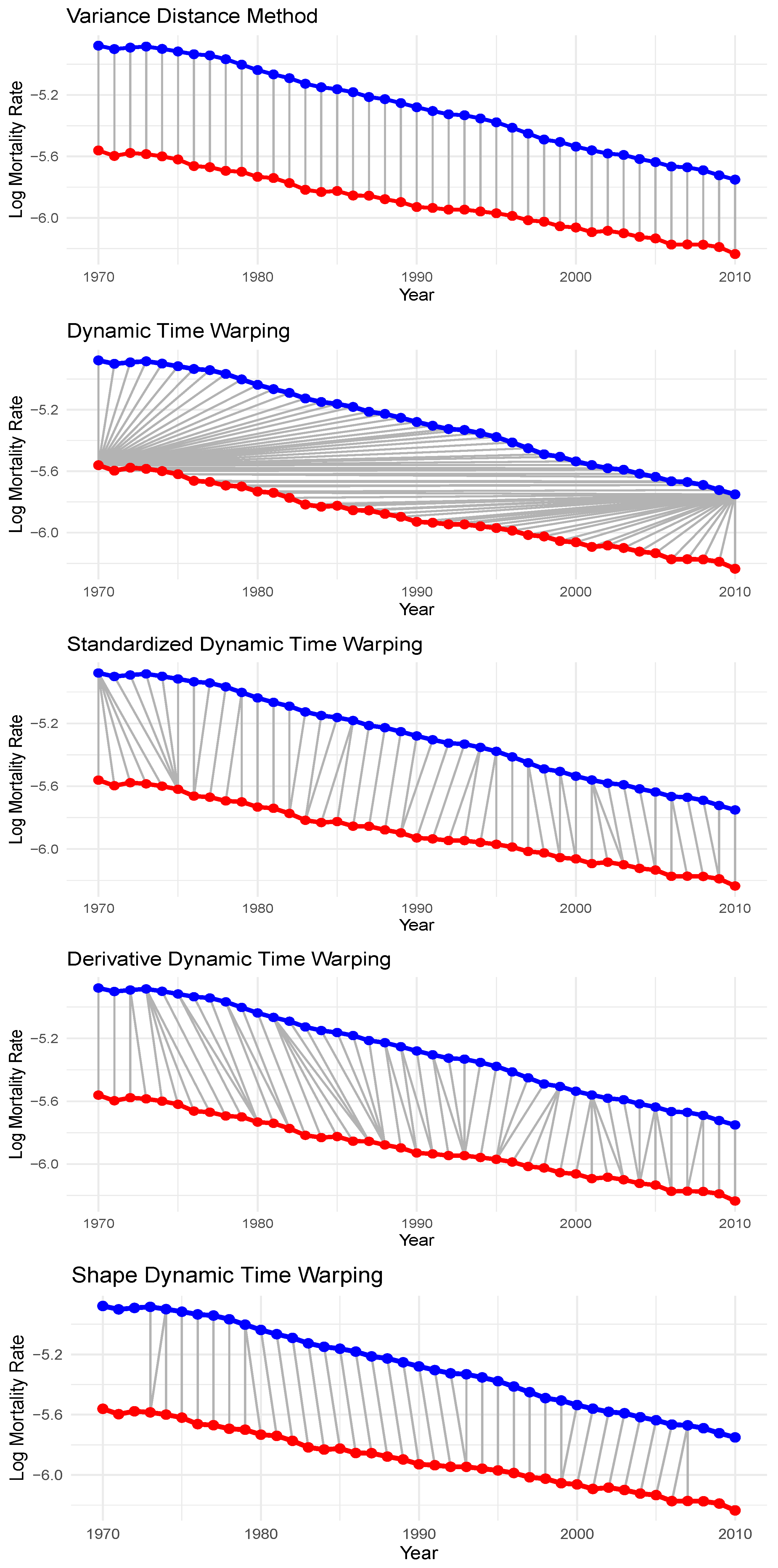
The results in the table clearly provide some insights regarding the selection of different distance functions and the linkage functions. In terms of the mean test SSEs, the proposed methods outperform the benchmark approaches in most cases, as reflected by their lower mean SSE values for both female and male populations. The relatively inferior performance of the DTW-based method can be attributed to potential unintuitive temporal alignments for certain data, as illustrated in Figure 2. In contrast, the refined DTW-based approaches mitigate these shortcomings and achieve substantially improved performance, comparable to that of the variance-based method. Although the mean test SSEs provides a direct measure of the overall predictive accuracy, the other summary statistics reported in the table are also informative for distinguishing performance across methods, as they better reflect robustness. Accordingly, we emphasize rank-based comparisons, summarized by the values in the “Average Rank” column, to assess the relative performance across methods. Based on these results, we recommend the ensemble approach, which averages all base learners using a simple mean, rather than selecting a single best-performing base learner. Because the identity of the best individual base learner varies across linkage functions and selection criteria, the SimAvg ensemble method exhibits more stable overall performance, with its average rank consistently being first or second among all methods. When comparing the linkage functions, we recommend the complete and average linkage methods over the other alternatives for two primary reasons. First, as discussed in Section 2.2.4, complete linkage emphasizes global cohesion by defining groups as similar only when all pairwise distances are small, while average linkage strikes a balance between local and global similarities. Consequently, both methods are less susceptible to undue influences from isolated close pairs arising from noise. Second, based on the comparison of the mean test SSEs reported in the tables, the SimAvg ensemble method exhibits superior predictive performance when either complete or average linkage is employed.

The superiority of the SimAvg ensemble method is further supported by the following results of the one-sided Diebold–Mariano (DM) test, which was introduced by Diebold and Mariano (1995) and Harvey et al. (1997) to formally compare the predictive accuracy of two predicting models. Let $M_1$ and $M_2$ denote the models under comparison; the general procedure of the one-sided DM test can be described as follows.

(1)

Calculate the forecast errors, defined as $e_{i,t}=y_t-{\widehat{y}}_{i,t}(\mathrm{for}\mathrm{model}{M}_i)\mathrm{i}=1,2$, where $y_t$ is the actual value and ${\widehat{y}}_{i,t}$ is the forecast from model i.

(2)

Calculate the loss differential $d_t=L\left(e_{1,t}\right)-L\left(e_{2,t}\right)$, where L is a loss function, commonly taken to be the squared error loss $L\left(e\right)=e^2$.

(3)

Calculate the DM test statistic $DM={\displaystyle \frac{\overline{d}}{s_d/\sqrt{T}}}$, where the mean of the loss differentials is calculated as

$$\overline{d}={\displaystyle \frac{1}{T}}\sum _{t=1}^T{d}_t$$

with T being the number of forecasts, and the variance in the loss differential is calculated as

$$s_d^2={\displaystyle \frac{1}{T-1}}\sum _{t=1}^T{(d_t-\overline{d})}^2$$

(4)

Impose the following one-side test hypotheses:

$$H_0:E\left[d_t\right]\le 0\mathrm{vs}{H}_a:E\left(d_t\right)>0.$$

Assume that the loss differentials $\{d_1,\cdots ,d_T\}$ are stationary in the sense that they have the same mean and variance. Then, under the null hypothesis, the test statistic $DM$ follows a standard normal distribution as T approaches infinity. If the calculated $DM$ statistic exceeds the critical value from the normal distribution, one would reject the null hypothesis, concluding that model $M_2$ provides significantly better predictions than model $M_1$ since the expected value of the loss differential is negative.

We compare the prediction accuracy of each benchmark model against its corresponding model from the proposed method using two one-sided Diebold–Mariano (DM) tests based on the age-aggregated test SSEs. If the first null hypothesis that the benchmark model is no better than the proposed model is rejected, we conclude that the benchmark model performs better and therefore wins the comparison. Conversely, if the second null hypothesis that the proposed model is no better than the benchmark is rejected, the proposed model is deemed superior. If neither hypothesis is rejected, the comparison results in a tie. For each model pair, this win determination process is repeated across all 288 predicting targets, and a higher frequency of wins reflects better predictive performance. In

Table 5. Number of wins for comparisons between the proposed models with (rows) and the Lee-Carter benchmark models (columns) based on pairs of one-sided DM tests. In each cell, the first integer indicates the number of wins for the proposed model and the second integer indicates the number of wins for the benchmark model.

	LCAllAges	LCOneAge
Female Population
LC-VarianceDiff-Centroid	(69,  29)	(44,  37)
LC-SimAvg-Centroid	(73,  29)	(52,  33)
LC-VarianceDiff-Single	(74,  28)	(31,  36)
LC-SimAvg-Single	(70,  32)	(47,  40)
LC-VarianceDiff-Complete	(69,  34)	(38,  31)
LC-SimAvg-Complete	(70,  26)	(57,  25)
LC-VarianceDiff-Average	(71,  29)	(43,  30)
LC-SimAvg-Average	(72,  31)	(53,  25)
Male Population
LC-VarianceDiff-Centroid	(86,  17)	(58,  26)
LC-SimAvg-Centroid	(91,  19)	(59,  32)
LC-VarianceDiff-Single	(84,  21)	(48,  19)
LC-SimAvg-Single	(85,  20)	(56,  29)
LC-VarianceDiff-Complete	(77,  23)	(60,  19)
LC-SimAvg-Complete	(85,  21)	(68,  30)
LC-VarianceDiff-Average	(79,  22)	(58,  27)
LC-SimAvg-Average	(88,  17)	(62,  39)

, we present the comparison results between the two groups of models, where the proposed age grouping models appear in the rows and the benchmark models in the columns. Each cell contains two integers: the first indicates the number of wins for the model in the row, and the second indicates the number of wins for the model in the column. To keep the comparison concise, we report only results for the base learners using a variance-based distance measure with different linkage choices, as the base learners using other distance measures (except for the original DTW) exhibit very similar performance. We also include the models that incorporate the simple averaging procedure in the comparison against the benchmarks.

The results from Table 5 indicate that the VarianceDiff and SimAvg models, under different linkage functions, generally perform better than the benchmark models in terms of predictive accuracy, as reflected by their larger numbers of successes across most entries (except for LC-VarianceDiff-Single against LCOneAge). Moreover, the SimAvg method secures more DM test victories over the benchmarks than the VarianceDiff method. This again underscores the advantage of incorporating the ensemble-based simple averaging procedure, which strengthens the predictive performance by delivering more statistically robust outperformance relative to the benchmarks.

The DM test comparison results between the two groups of models across different age groups are further presented in

Table 6. Number of wins for comparisons between the proposed models (rows) and the benchmark models (columns) for different age groups based on pairs of one-sided DM tests. In each cell, the first integer indicates the number of wins for the proposed model and the second integer indicates the number of wins for the benchmark model.

Infant			Kid
	LCAllAges	LCOneAge		LCAllAges	LCOneAge
LC-VarianceDiff-Centroid	(39, 4)	(19, 10)	LC-VarianceDiff-Centroid	(26, 3)	(18, 6)
LC-SimAvg-Centroid	(42, 2)	(19, 15)	LC-SimAvg-Centroid	(28, 3)	(19, 6)
LC-VarianceDiff-Single	(42, 1)	(16, 11)	LC-VarianceDiff-Single	(29, 4)	(16, 4)
LC-SimAvg-Single	(41, 3)	(18, 16)	LC-SimAvg-Single	(21, 6)	(16, 10)
LC-VarianceDiff-Complete	(40, 1)	(22, 5)	LC-VarianceDiff-Complete	(27, 1)	(22, 3)
LC-SimAvg-Complete	(41, 1)	(22, 9)	LC-SimAvg-Complete	(26, 2)	(24, 5)
LC-VarianceDiff-Average	(40, 1)	(22, 7)	LC-VarianceDiff-Average	(29, 1)	(22, 3)
LC-SimAvg-Average	(41, 1)	(23, 9)	LC-SimAvg-Average	(27, 5)	(21, 7)
Teen			Adult
	LCAllAges	LCOneAge		LCAllAges	LCOneAge
LC-VarianceDiff-Centroid	(14, 7)	(17, 4)	LC-VarianceDiff-Centroid	(31, 6)	(13, 15)
LC-SimAvg-Centroid	(13, 11)	(20, 4)	LC-SimAvg-Centroid	(32, 9)	(14, 16)
LC-VarianceDiff-Single	(14, 8)	(14, 3)	LC-VarianceDiff-Single	(29, 10)	(6, 13)
LC-SimAvg-Single	(13, 10)	(17, 5)	LC-SimAvg-Single	(28, 10)	(14, 15)
LC-VarianceDiff-Complete	(11, 12)	(14, 5)	LC-VarianceDiff-Complete	(30, 10)	(7, 9)
LC-SimAvg-Complete	(13, 10)	(15, 6)	LC-SimAvg-Complete	(31, 9)	(21, 15)
LC-VarianceDiff-Average	(12, 10)	(17, 6)	LC-VarianceDiff-Average	(27, 11)	(9, 12)
LC-SimAvg-Average	(14, 10)	(16, 7)	LC-SimAvg-Average	(30, 11)	(13, 19)
Retiree			Old
	LCAllAges	LCOneAge		LCAllAges	LCOneAge
LC-VarianceDiff-Centroid	(29, 11)	(10, 17)	LC-VarianceDiff-Centroid	(16, 15)	(25, 11)
LC-SimAvg-Centroid	(29, 10)	(13, 17)	LC-SimAvg-Centroid	(20, 13)	(26, 7)
LC-VarianceDiff-Single	(29, 10)	(6, 12)	LC-VarianceDiff-Single	(15, 16)	(21, 12)
LC-SimAvg-Single	(30, 10)	(13, 13)	LC-SimAvg-Single	(22, 13)	(25, 10)
LC-VarianceDiff-Complete	(25, 15)	(9, 14)	LC-VarianceDiff-Complete	(13, 18)	(24, 14)
LC-SimAvg-Complete	(28, 10)	(18, 13)	LC-SimAvg-Complete	(16, 15)	(25, 7)
LC-VarianceDiff-Average	(24, 14)	(8, 17)	LC-VarianceDiff-Average	(18, 14)	(23, 12)
LC-SimAvg-Average	(29, 12)	(14, 16)	LC-SimAvg-Average	(19, 9)	(28, 6)

for more detailed decomposition across different age groups. Across all age groups, SimAvg with complete linkage consistently outperforms the benchmarks in most cases, but the strength of its dominance varies across ages.

• When compared with LCAllAges, all SimAvg methods record a substantial number of wins for the infant, kid, adult, and retiree age groups. For the teen and old groups, the wins still exceed the losses, although the margin narrows, and, in some cases, it approaches parity. This pattern is broadly consistent with intuitive expectations regarding data availability and information sharing across age groups. In particular, infant mortality exhibits distinct dynamics, while adult and retiree ages tend to display relatively stable patterns supported by large exposure sizes, limiting the effectiveness of excessive pooling. In contrast, the teen and old age groups are characterized by higher volatility and smaller exposure sizes, leading them to benefit more from information borrowed across ages, which makes LCAllAges relatively more competitive in these ranges. Nevertheless, the proposed SimAvg approach continues to deliver robust improvements overall, with especially pronounced gains observed at very young and middle ages.
• When compared with LCOneAge, the SimAvg methods exhibit pronounced improvements for the infant, kid, teen, and old age groups, particularly under complete and average linkages. In contrast, the results for the adult and retiree groups are mixed, with several SimAvg methods recording more losses than wins against LCOneAge. Nevertheless, when complete linkage is employed, the proposed ensemble approach continues to achieve a net advantage over LCOneAge.

Overall, SimAvg with complete linkage demonstrates clear improvements over LCAllAges for most age groups, while its advantages over LCOneAge are primarily concentrated at the youngest and oldest ages; for the adult and retiree groups, the evidence of improvement is less pronounced.

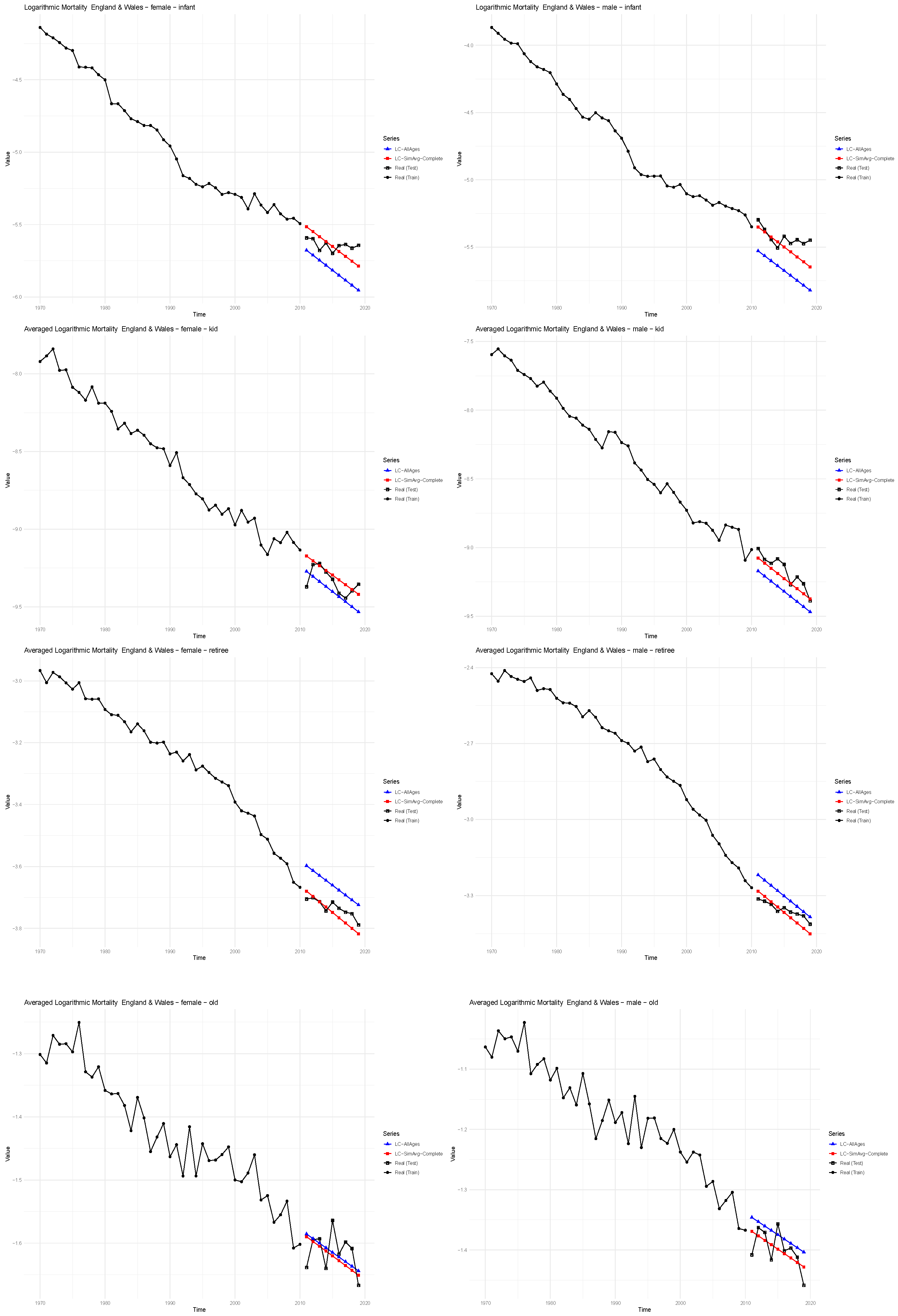
To illustrate cases in which our approach performs particularly well, we consider the male and female populations of England and Wales as representative examples to compare the proposed ensemble-based model (LC-SimAvg-Complete) with the benchmark Lee–Carter model (LCAllAges). Figure 4 displays the observed and forecasted average logarithmic mortality rates for the infant, child, retiree, and old age groups under both models. As noted earlier, the training sample covers the period 1970–2010, while the out-of-sample evaluation spans 2011–2019. The results show that the proposed method generally aligns more closely with the realized mortality rates, or performs at least comparably to the Lee–Carter model, across all targets presented, indicating the practical significance of the proposed method in terms of enhancing mortality predictions.

3.3. Stylized Facts in Reference Selections

In this subsection, we summarize several stylized facts regarding how, for different age groups, reference datasets are selected and information is borrowed in distinct ways. The findings in (Meng et al. 2025) reveal a clear pattern in the amount of external data borrowed as the target age varies from 0 to 100. Middle-age groups tend to benefit from borrowing information from a moderate number of adjacent ages, which improves the prediction accuracy without introducing unnecessary noise. In contrast, both younger and older ages typically require information from a broader range of neighboring ages due to greater variability in their mortality patterns. Infants, however, tend to borrow from a smaller set of nearby ages, as their mortality behaviors are highly unique and do not gain much from incorporating a large number of reference ages. 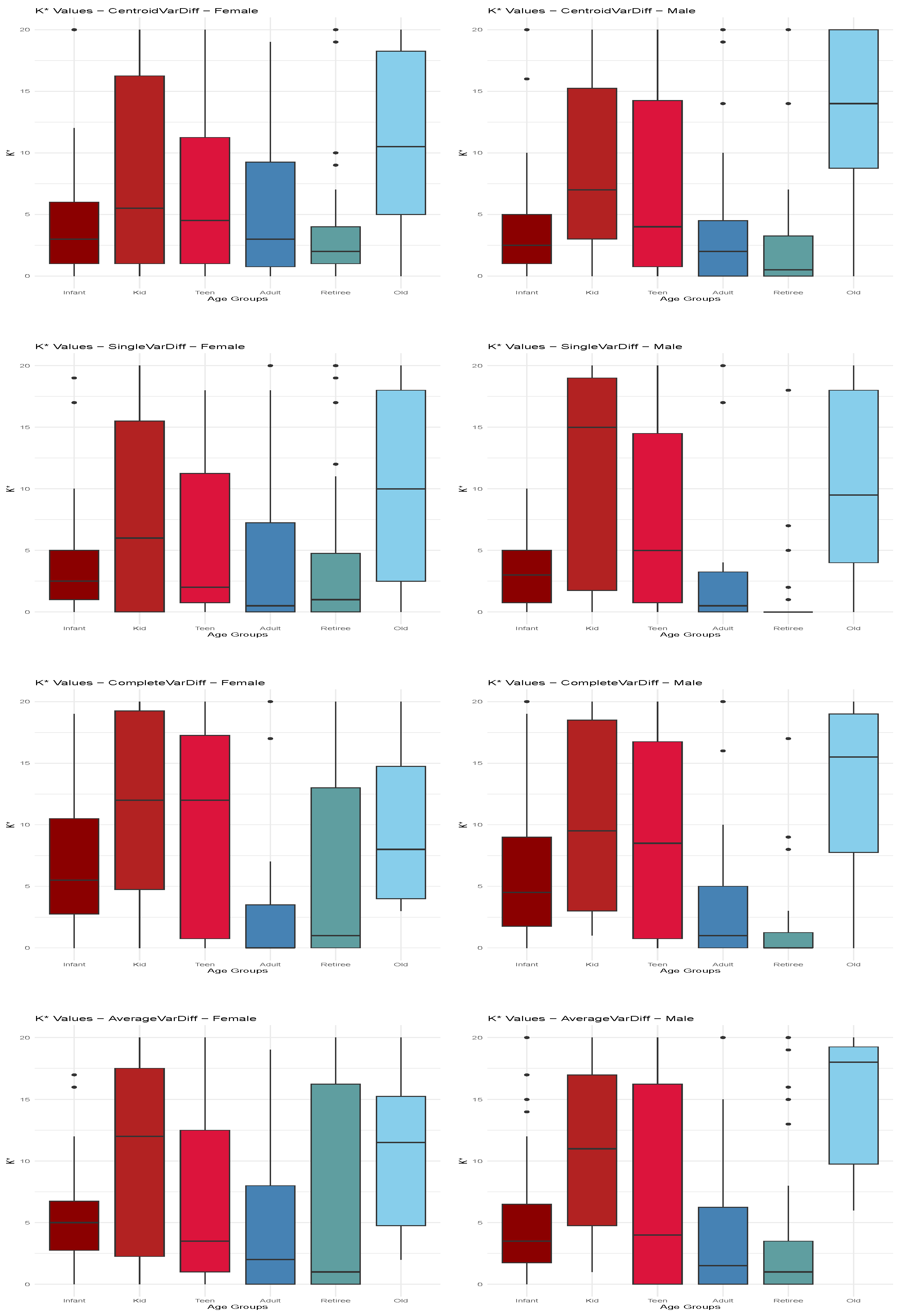Since the selected value of k from the proposed method represents the optimal number of reference groups used for each target population–gender–age group $G_T=(B_i,p_j,g_k)$, we present boxplots of the optimal chosen values of k for each gender–age combination across all target populations from the VarianceDiff-Centroid method in Figure 5. This visualization highlights the overall pattern in how many external reference age groups are incorporated to achieve the best predictive performance for each target group.

The averaged chosen optimal k values for each gender–age combination across all target populations, shown in Figure 5, reveal a consistent pattern, regardless of the chosen linkage method, illustrating how much external information each group borrows, as also noted in (Meng et al. 2025). Specifically, the infant, adult, and retiree age groups, on average, tend to borrow less from other data, whereas the kid, teen, and old age groups incorporate a greater amount. The differences in the box widths in Figure 5 further illustrate the degree of variation in the optimal amount of external data across gender–age combinations. The infant and retiree age groups exhibit noticeably narrower boxes, indicating greater stability in the selected values of k, which represent the optimal number of reference groups used to enhance the predictive performance. In contrast, the adult and teenage groups show more variability across populations, reflected by their wider box widths, while the kid and old age groups display the largest variability in the chosen k values in all figures. Overall, this suggests that the infant and retiree groups across all populations tend to consistently select relatively small numbers of reference groups, whereas other age groups generally rely on larger and more variable amounts of external data, with the results differing from one population to another.

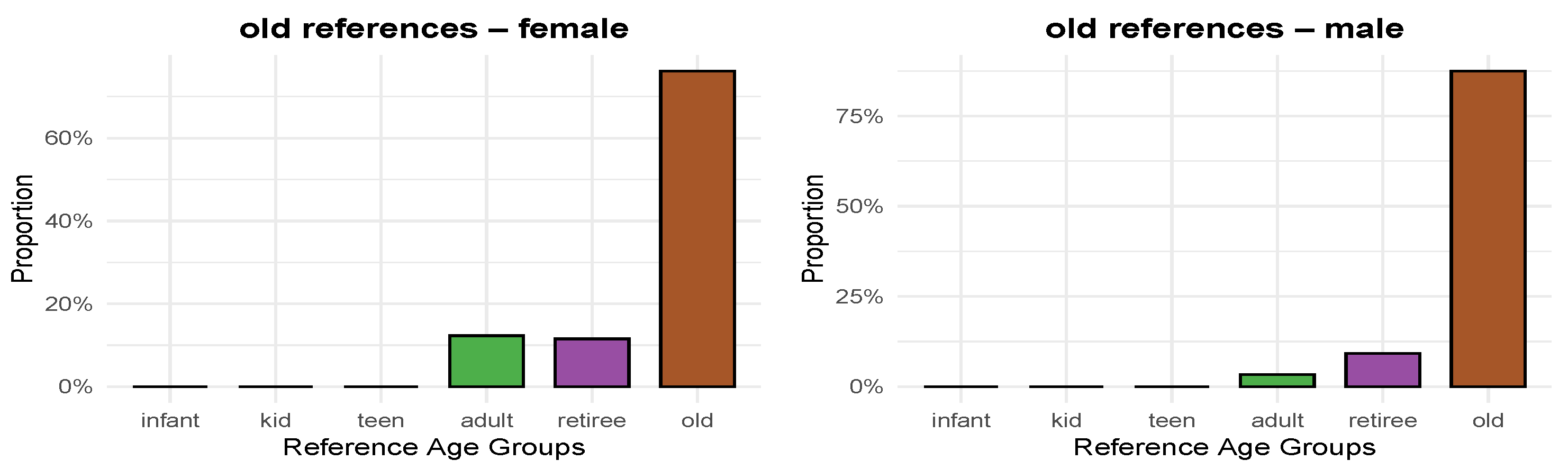
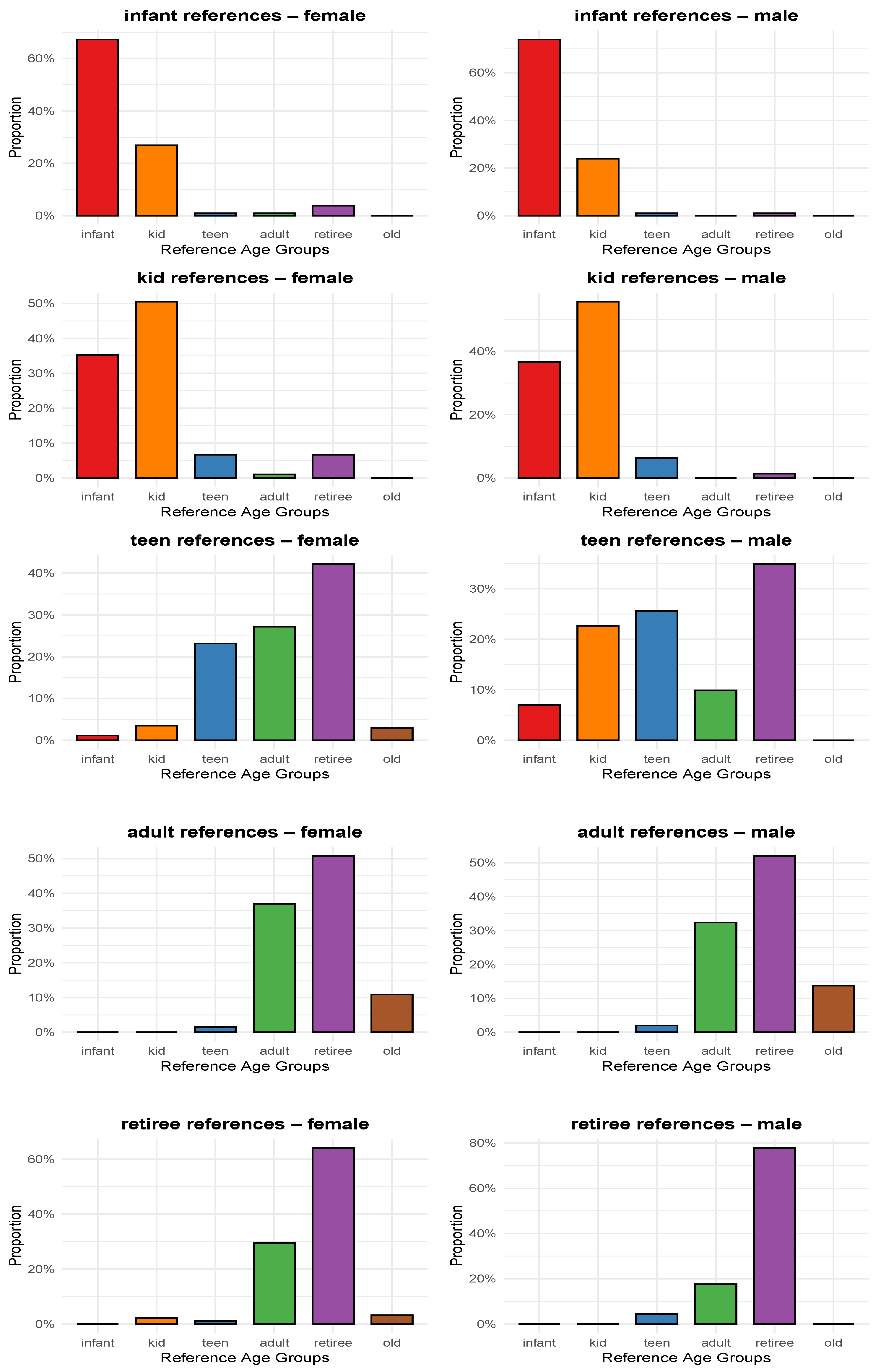
We also analyze the age group compositions of the reference sets for different targets by calculating the average realized percentages of age groups selected by the proposed method (with the variance-based distance and centroid linkage functions) for each of the six target age groups across all 24 populations and both genders, as shown in Figure 6. The visualizations illustrate the specific role that each age group plays within the system of information flow, as outlined below.

• Target age groups tend to draw a substantial portion of their references from their own corresponding age groups across all populations. This pattern is especially pronounced for the infant, kid, retiree, and old age groups, where the same age groups across populations consistently constitute the largest share of the selected references.
• As the reference age group moves further away from the target age group, it becomes less likely to be included in the selected reference set. This is evident from the consistently small proportions of the old age groups chosen as references when the target is infants or kids, and vice versa.
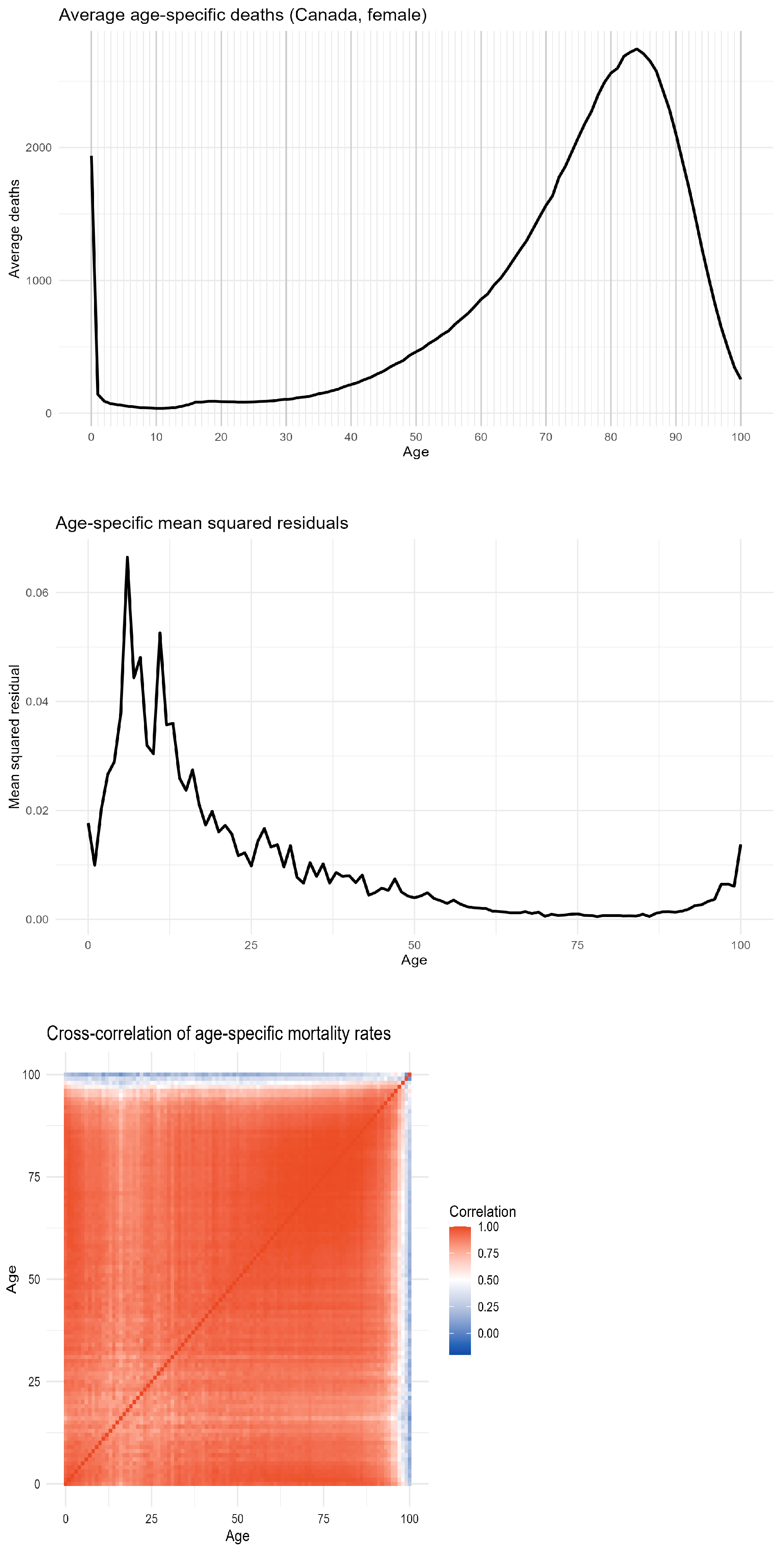
• Unlike most other age groups, the retiree age groups stand out by appearing more frequently in the selected reference sets. Indeed, they even constitute the largest proportion of references for the teen and adult target groups. This suggests that the retiree age groups provide more universal information that can be effectively borrowed by a wide range of other age groups. Although this may sound counterintuitive at first glance, it arises naturally within mortality modeling framework, with several reasons. First, from a credibility perspective, the retiree age group has mortality data with large exposures and correspondingly low variance, making these rates statistically more reliable. Consequently, when predicting mortality for other age groups, the procedure tends to borrow more information from these highly credible sources to reduce estimation uncertainty. Second, the contribution reflects genuine alignment in mortality trends across age groups over time. In particular, the sequences of period effects $k_t$ for the retiree groups tend to be closely correlated with those of other age groups, which allows the joint modeling procedure to borrow meaningful information across ages. To illustrate this graphically, we have plotted the age-specific number of deaths (representing exposure), the age-specific average of the realized squared residuals for Canadian females, and the cross-correlation heatmap between age-specific log-mortality rate sequences, which are presented in Figure 7. The graphs reveal clear patterns across ages. First, the total number of deaths is dominated by the retiree age group, with the peak also occurring within this group, reflecting their large exposures. Second, the residuals are generally homoskedastic across most ages, with an upward trend at the oldest ages, indicating variance inflation, and occasional peaks at young and working ages. In contrast, the residuals remain small and stable for the retiree age groups, suggesting lower volatility in their mortality rate sequences. Moreover, the cross-correlation between age-specific log-mortality rate sequences is obviously positive for most pairs of ages; with only the very old age (near 100), the correlation becomes less positive.

3.4. Extending to LC2 Model

Another key factor influencing the effectiveness of mortality prediction is the choice of the underlying mortality model, which has been extensively examined throughout the literature (e.g., Cairns et al. 2009; Li et al. 2015; Li and Lee 2005; Yang et al. 2016). In the preceding subsection, we embedded the classic Lee–Carter model into the age grouping framework under various distance measuring and linkage functions. This choice is natural because the selected reference population–gender–age groups are assumed to share a consistent underlying time trend with the target group, albeit potentially evolving at slightly different speeds. In this subsection, we introduce greater flexibility by replacing the embedded mortality model with a more complex alternative. This serves two purposes. First, we aim to explore whether a more flexible model can consistently enhance the predictive accuracy across different population–gender–age target groups. Second, we seek to assess the ability of our age grouping-based methods to integrate with alternative mortality models. To balance model complexity and implementation feasibility, we focus on the LC2 model, which sets the number of effect components $S=2$ as in Equation (3). The LC2 model has two pairs of age/period effects $(b_x^{\left(1\right)},k_t^{\left(1\right)})$ and $(b_x^{\left(2\right)},k_t^{\left(2\right)})$ to capture a more complex shared time trend across all included age groups, along with their relative rates of evolution.

The numerical comparison adopts the same HMD data and includes the benchmark “AllAges” and “OneAge” methods and the proposed VarianceDiff and SimAvg methods, using both Lee–Carter and LC2 as the underlying mortality models. This setup allows us to comprehensively assess the proposed methods relative to the benchmarks, including comparisons across different underlying mortality models and evaluations of the ensemble-based strategies against individual base learners. The comparison follows the same strategy as in Section 3.2, and we report the first quartile, median, sample mean, and third quartile for the overall test SSEs across all target population–gender–age groups $G_T$, ranking the relative performance and calculating the average rank for each row. The results are presented in

Table 7. Summary statistics of test SSEs for prediction performance of complete linkage models for genders and all age groups combined. Numbers in parentheses indicate the rank of predicting performance for each reported summary statistic of test SSEs for genders and all age groups combined. Lower ranks indicate better performance.

	1st Quartile	Median	Mean	3rd Quartile	Average Rank
Female Population
LCAllAges	0.7649 (8)	3.4817 (7)	10.1457 (8)	17.7492 (5)	(7.00)
LCOneAge	0.4747 (3)	2.8163 (4)	10.1414 (7)	18.9084 (8)	(5.50)
LC2AllAges	0.7152 (7)	3.4818 (8)	10.1202 (6)	17.7492 (5)	(6.50)
LC2OneAge	0.4751 (4)	2.8066 (3)	9.9736 (5)	18.7978 (7)	(4.75)
LC-VarianceDiff-Complete	0.5128 (6)	2.8721 (5)	9.5625 (4)	17.7030 (4)	(4.75)
LC2-VarianceDiff-Complete	0.4770 (5)	3.1268 (6)	9.4957 (2)	17.2126 (2)	(3.75)
LC-SimAvg-Complete	0.4601 (1)	2.7116 (2)	9.5623 (3)	17.5600 (3)	(2.25)
LC2-SimAvg-Complete	0.4662 (2)	2.6283 (1)	9.3890 (1)	16.9173 (1)	(1.25)
Male Population
LCAllAges	1.0711 (8)	3.4144 (6)	9.8425 (8)	14.6982 (7)	(7.25)
LCOneAge	0.5861 (4)	4.2055 (8)	8.6163 (6)	12.6091 (6)	(6.00)
LC2AllAges	0.9521 (7)	3.1226 (5)	9.7300 (7)	14.6982 (7)	(6.50)
LC2OneAge	0.5539 (2)	3.6654 (7)	8.2065 (5)	11.3960 (3)	(4.25)
LC-VarianceDiff-Complete	0.5971 (5)	2.5408 (2)	7.8771 (4)	12.1424 (5)	(4.00)
LC2-VarianceDiff-Complete	0.5492 (1)	2.5572 (3)	7.6510 (2)	11.1547 (2)	(2.00)
LC-SimAvg-Complete	0.6250 (6)	2.6029 (4)	7.8758 (3)	11.9907 (4)	(4.25)
LC2-SimAvg-Complete	0.5657 (3)	2.5207 (1)	7.4883 (1)	10.7497 (1)	(1.50)

and

Table 8. Summary statistics of test SSEs for prediction performance of average linkage models for genders and all age groups combined. Numbers in parentheses indicate the rank of predicting performance for each reported summary statistic of test SSEs for genders and all age groups combined. Lower ranks indicate better performance.

	1st Quartile	Median	Mean	3rd Quartile	Average Rank
Female Population
LCAllAges	0.7649 (8)	3.4817 (6)	10.1457 (8)	17.7492 (4)	(6.50)
LCOneAge	0.4747 (3)	2.8163 (3)	10.1414 (7)	18.9084 (8)	(5.25)
LC2AllAges	0.7152 (7)	3.4818 (7)	10.1202 (6)	17.7492 (4)	(6.00)
LC2OneAge	0.4751 (4)	2.8066 (2)	9.9736 (5)	18.7978 (7)	(4.50)
LC-VarianceDiff-Average	0.5063 (6)	2.9145 (4)	9.5862 (3)	17.7205 (3)	(4.00)
LC2-VarianceDiff-Average	0.5010 (5)	3.5335 (8)	9.5485 (2)	18.2422 (6)	(5.25)
LC-SimAvg-Average	0.4702 (2)	2.6805 (1)	9.6475 (4)	17.5747 (2)	(2.25)
LC2-SimAvg-Average	0.4491 (1)	3.0019 (5)	9.5360 (1)	17.4697 (1)	(2.00)
Male Population
LCAllAges	1.0711 (8)	3.4144 (6)	9.8425 (8)	14.6982 (7)	(7.25)
LCOneAge	0.5861 (5)	4.2055 (8)	8.6163 (6)	12.6091 (6)	(6.25)
LC2AllAges	0.9521 (7)	3.1226 (5)	9.7300 (7)	14.6982 (7)	(6.50)
LC2OneAge	0.5539 (3)	3.6654 (7)	8.2065 (5)	11.3960 (2)	(4.25)
LC-VarianceDiff-Average	0.5814 (4)	2.7794 (4)	7.8010 (3)	12.2515 (5)	(4.00)
LC2-VarianceDiff-Average	0.5225 (2)	2.6302 (2)	7.4728 (1)	11.4458 (3)	(2.00)
LC-SimAvg-Average	0.5936 (6)	2.7153 (3)	7.8952 (4)	11.8502 (4)	(4.25)
LC2-SimAvg-Average	0.5188 (1)	2.5572 (1)	7.4938 (2)	10.8463 (1)	(1.25)

for the complete and average linkage methods, whereas the corresponding results for the centroid and single linkage methods are provided in

Table A3. Summary statistics of test SSEs for prediction performance of centroid linkage models for genders and all age groups combined. Numbers in parentheses indicate the rank of predicting performance for each reported summary statistic of test SSEs for genders and all age groups combined. Lower ranks indicate better performance.

	1st Quartile	Median	Mean	3rd Quartile	Average Rank
Female Population
LCAllAges	0.7649 (8)	3.4817 (7)	10.1457 (8)	17.7492 (4)	(6.75)
LCOneAge	0.4747 (2)	2.8163 (3)	10.1414 (7)	18.9084 (8)	(4.75)
LC2AllAges	0.7152 (7)	3.4818 (8)	10.1202 (6)	17.7492 (4)	(6.25)
LC2OneAge	0.4751 (3)	2.8066 (2)	9.9736 (5)	18.7978 (7)	(4.25)
LC-VarianceDiff-Centroid	0.4839 (5)	2.8950 (4)	9.6096 (2)	16.7116 (1)	(3.00)
LC2-VarianceDiff-Centroid	0.5053 (6)	3.1130 (6)	9.7791 (4)	18.6104 (6)	(5.50)
LC-SimAvg-Centroid	0.4836 (4)	2.7705 (1)	9.6277 (3)	17.3743 (3)	(2.75)
LC2-SimAvg-Centroid	0.4597 (1)	2.9470 (5)	9.5300 (1)	16.9777 (2)	(2.25)
Male Population
LCAllAges	1.0711 (8)	3.4144 (6)	9.8425 (8)	14.6982 (7)	(7.25)
LCOneAge	0.5861 (3)	4.2055 (8)	8.6163 (6)	12.6091 (5)	(5.50)
LC2AllAges	0.9521 (7)	3.1226 (5)	9.7300 (7)	14.6982 (7)	(6.50)
LC2OneAge	0.5539 (1)	3.6654 (7)	8.2065 (5)	11.3960 (2)	(3.75)
LC-VarianceDiff-Centroid	0.5904 (4)	2.7464 (4)	7.8950 (3)	12.8546 (6)	(4.25)
LC2-VarianceDiff-Centroid	0.6492 (6)	2.4392 (2)	7.6295 (2)	11.5304 (3)	(3.25)
LC-SimAvg-Centroid	0.6289 (5)	2.6668 (3)	7.9028 (4)	12.3427 (4)	(4.00)
LC2-SimAvg-Centroid	0.5806 (2)	2.4296 (1)	7.5707 (1)	11.2919 (1)	(1.25)

and

Table A4. Summary statistics of test SSEs for prediction performance of simple linkage models for genders and all age groups combined. Numbers in parentheses indicate the rank of predicting performance for each reported summary statistic of test SSEs for genders and all age groups combined. Lower ranks indicate better performance.

	1st Quartile	Median	Mean	3rd Quartile	Average Rank
Female Population
LCAllAges	0.7649 (8)	3.4817 (6)	10.1457 (8)	17.7492 (1)	(5.75)
LCOneAge	0.4747 (4)	2.8163 (3)	10.1414 (7)	18.9084 (8)	(5.50)
LC2AllAges	0.7152 (7)	3.4818 (7)	10.1202 (6)	17.7492 (1)	(5.25)
LC2OneAge	0.4751 (5)	2.8066 (2)	9.9736 (4)	18.7978 (7)	(4.50)
LC-VarianceDiff-Single	0.4543 (3)	3.5040 (8)	9.7569 (2)	17.7620 (3)	(4.00)
LC2-VarianceDiff-Single	0.4943 (6)	3.2220 (5)	10.0516 (5)	18.1202 (5)	(5.25)
LC-SimAvg-Single	0.4445 (2)	2.7497 (1)	9.7220 (1)	17.7663 (4)	(2.00)
LC2-SimAvg-Simple	0.4327 (1)	2.9411 (4)	9.7804 (3)	18.7487 (6)	(3.50)
Male Population
LCAllAges	1.0711 (8)	3.4144 (6)	9.8425 (8)	14.6982 (7)	(7.25)
LCOneAge	0.5861 (2)	4.2055 (8)	8.6163 (6)	12.6091 (5)	(5.25)
LC2AllAges	0.9521 (7)	3.1226 (4)	9.7300 (7)	14.6982 (7)	(6.25)
LC2OneAge	0.5539 (1)	3.6654 (7)	8.2065 (5)	11.3960 (1)	(3.50)
LC-VarianceDiff-Single	0.6591 (5)	3.1409 (5)	7.8820 (2)	11.4772 (2)	(3.50)
LC2-VarianceDiff-Single	0.6591 (5)	2.8667 (2)	8.0406 (4)	12.8475 (6)	(4.25)
LC-SimAvg-Single	0.6351 (3)	2.9061 (3)	8.0147 (3)	11.9080 (4)	(3.25)
LC2-SimAvg-Simple	0.6379 (4)	2.4958 (1)	7.7113 (1)	11.5104 (3)	(2.25)

in the Appendix A.

Across both linkage strategies and genders, the benchmark LC models exhibit the weakest predictive performance, while the proposed ensemble-based LC2 models consistently achieve superior accuracy and robustness. Although the LC2AllAges and LC2OneAge benchmarks improve upon their LC counterparts, they remain clearly dominated by the ensemble LC2 approaches, indicating that the main performance gains arise from the aggregation mechanisms rather than from the LC2 extension alone. Interestingly, the simpler LCOneAge model is often competitive with—and in some cases outperforms—LC2AllAges, suggesting that increased model complexity does not automatically translate into better predictive accuracy. Overall, the results underscore the importance of targeted conditioning through the selection of reference ages, together with ensemble strategies that combine predictions from multiple base learners, in achieving consistent improvements in mortality forecasting performance.

The superiority of the SimAvg ensemble method is further supported by the pairwise comparison results based on the DM test, presented in

Table 9. Number of wins for comparisons between the proposed models (rows) and the benchmark LC2 models (columns) based on pairs of one-sided DM tests. In each cell, the first integer indicates the number of wins for the proposed model and the second integer indicates the number of wins for the benchmark model.

	LC2AllAges	LC2OneAge
Female Population
LC2-VarianceDiff-Centroid	(60,  33)	(37,  38)
LC2-SimAvg-Centroid	(66,  27)	(57,  32)
LC2-VarianceDiff-Single	(65,  24)	(27,  26)
LC2-SimAvg-Single	(67,  29)	(52,  35)
LC2-VarianceDiff-Complete	(65,  29)	(37,  28)
LC2-SimAvg-Complete	(73,  20)	(59,  24)
LC2-VarianceDiff-Average	(62,  28)	(39,  34)
LC2-SimAvg-Average	(70,  28)	(55,  35)
Male Population
LC2-VarianceDiff-Centroid	(76,  20)	(50,31)
LC2-SimAvg-Centroid	(83,21)	(60,39)
LC2-VarianceDiff-Single	(67,23)	(43,30)
LC2-SimAvg-Single	(74,17)	(52,33)
LC2-VarianceDiff-Complete	(73,25)	(49,32)
LC2-SimAvg-Complete	(87,16)	(64,36)
LC2-VarianceDiff-Average	(83,20)	(58,28)
LC2-SimAvg-Average	(88,14)	(59,33)

. In general, the proposed methods tend to outperform the benchmark models, as reflected by their larger numbers of wins in most comparisons (except LC2-VarianceDiff-Centroid against LC2OneAge). Moreover, when the same linkage function is used, the SimAvg method consistently achieves more DM test victories against the benchmarks than the VarianceDiff method, indicating further gains in predictive performance.

4. Concluding Remarks

This paper examines mortality prediction through a data filtering perspective and extends the individual age-specific framework of (Meng et al. 2025) to a more general age grouping-based prediction framework. The age grouping procedure partitions a population’s mortality data into distinct life stage-based age groups, allowing ages with similar mortality trajectories to be analyzed together while excluding ages that exhibit different mortality patterns due to belonging to different stages of life. A fully data-driven statistical learning algorithm is proposed to allow information between multiple populations, genders, and ages to be considered simultaneously based on the structural similarities among all population–gender–age groups. The introduction of multiple choices for both the distance measure and the linkage function overcomes the limitations of using single distance measures and aggregates the pairwise mortality-series similarities into an overall object-to-object distance, which determines the merging order of these population–gender–age groups. An additional ensemble-based model averaging procedure further enhances the effectiveness and robustness of the final results. Extensive empirical comparisons using the Human Mortality Database demonstrate both the predictive improvements achieved by the proposed method and its compatibility with different underlying mortality models, offering practitioners a versatile approach to modeling mortality at the age group level in real-world applications.

Although our specification of age groups remains, to some extent, pragmatic, fully data-driven age grouping schemes may have the potential to further tailor models to population-specific mortality dynamics. However, developing such grouping strategies in a way that delivers meaningful predictive improvements while maintaining computational efficiency, stability, and interpretability remains challenging. A systematic investigation of approaches that balance flexibility with structural coherence across populations therefore represents a promising direction for future research.