Article

Estimating Disease-Free Life Expectancy Based on Clinical Data from the French Hospital Discharge Database

by
Oleksandr Sorochynskyi
1,2,*,
Quentin Guibert
3,
Frédéric Planchet
1,2 and
Michaël Schwarzinger
4,5
1
Laboratoire SAF EA2429, Institut de Science Financière et d’Assurances (ISFA), Université Claude Bernard Lyon 1, University of Lyon, 69366 Lyon, France
2
Prim’Act Actuarial Consulting Firm, 42 Avenue de la Grande Armée, 75017 Paris, France
3
CEREMADE, Université Paris-Dauphine, Université PSL, CNRS, 75016 Paris, France
4
Department of Prevention, Bordeaux University Hospital, 33000 Bordeaux, France
5
University of Bordeaux, INSERM, BPH, U1219, I-Prev/PHARES, Certified Team under Ligue Contre le Cancer, CIC 1401, 33000 Bordeaux, France
*
Author to whom correspondence should be addressed.
Risks 2024, 12(6), 92; https://doi.org/10.3390/risks12060092
Submission received: 23 April 2024 / Revised: 29 May 2024 / Accepted: 30 May 2024 / Published: 3 June 2024

Abstract

:
The development of health indicators to measure healthy life expectancy (HLE) is an active field of research aimed at summarizing the health of a population. Although many health indicators have emerged in the literature as critical metrics in public health assessments, the methods and data to conduct this evaluation vary considerably in nature and quality. Traditionally, health data collection relies on population surveys. However, these studies, typically of limited size, encompass only a small yet representative segment of the population. This limitation can necessitate the separate estimation of incidence and mortality rates, significantly restricting the available analysis methods. In this article, we leverage an extract from the French National Hospital Discharge database to define health indicators. Our analysis focuses on the resulting Disease-Free Life Expectancy (Dis-FLE) indicator, which provides insights based on the hospital trajectory of each patient admitted to hospital in France during 2008–2013. Through this research, we illustrate the advantages and disadvantages of employing large clinical datasets as the foundation for more robust health indicators. We shed light on the opportunities that such data offer for a more comprehensive understanding of the health status of a population. In particular, we estimate age-dependent hazard rates associated with sex, alcohol abuse, tobacco consumption, and obesity, as well as geographic location. Simultaneously, we delve into the challenges and limitations that arise when adopting such a data-driven approach.

1. Introduction

Over the last century, life expectancy has significantly increased. However, this increase has also been accompanied by a rise in the duration of life spent in a state of dependency (Fries 1980; Gruenberg 2005). This underscores the importance of health indicators, such as Healthy Life Expectancy (HLE), in monitoring the overall health of a population. HLE is an umbrella term for a family of health indicators that calculate the expected number of years lived in various health states.
HLE is utilized at all levels of policymaking, from international to local. Organizations such as the World Health Organization (WHO) and the European Union (EU) incorporate health indicators—Healthy Life Expectancy (HALE) and Healthy Life Years (HLY), respectively—into their frameworks for assessing population health (Bogaert et al. 2018; WHO 2023). Another example is Japan, which has prioritized health as a key policy objective in recent years (Abe 2013).
Despite the consensus on the importance of health indicators, no universally used definition of health has emerged (Jagger et al. 2020, chap. 1). The complexity of defining a useful health concept and the multiplicity of existing health concepts and methods to calculate them are well documented (Kim et al. 2022). However, one aspect appears to remain invariant: the use of surveys.
Surveys are the main source of data on health status of a population (Jagger et al. 2020, chap. 5). Unlike mortality data, that are already available from national statistics agencies who collect them for administrative purposes, health data are harder to come by, and surveys provide the most readily available means of doing so. The use of survey data necessarily imposes limits on the data collected. For one, the cost of surveys limits the sample sizes. Constructing survey instruments to be comparable over large areas is challenging (Robine 2003). Moreover, self-evaluation of health is influenced by various factors and can therefore be biased (Kempen et al. 1996; Krause and Jay 1994; Peersman et al. 2012). Finally, survey data also do not provide reliable mortality data.
At the same time, the introduction of electronic health records (EHRs) and international diagnostic harmonization has enabled the collection of medical information across large populations, with datasets like the United States’ National Hospital Care Survey, the United Kingdom’s Hospital Episode Statistics database, and Denmark’s National Patient Registry. In this paper, we focus on a subset of the French National Hospital Discharge database (Programme de Médicalisation des Systèmes d’Information). These data cover all hospital discharges from 2010 to 2013 for adults aged 50 and older, and cover, after all exclusions, 10 million unique patients. Each discharge contains the main discharge diagnosis, coded using ICD-10, a standardized international classification of diagnoses (World Health Organization 2015), as well as some demographic information on the patient.
We propose using such large clinical databases to construct health indicators. This proposed approach has many advantages for assessing the health status of a population. First, the use of standardized discharge diagnosis codes, like the ICD-10, simplifies and reinforces cross-regional and temporal comparisons. Second, the involvement of healthcare professionals in diagnosis minimizes biases associated with self-assessment. As the entire population is included, the database can provide a longitudinal view over a lifetime of diagnoses to create a comprehensive health picture. Finally, the individual-level data that contain information on both morbidity and mortality avoids the need for aggregating and allows for a more nuanced analysis, promising a more profound view of health.
Nonetheless, the clinical view of health has inherent limitations. First, a clinical view of health corresponds necessarily to a negative concept of health, considered inadequate by some (Jagger et al. 2020, chap. 1). In clinical settings, the focus is diagnosis and treatment, not holistic health assessment. This divergence yields several notable consequences (Euro-REVES et al. 2000). For instance, preventive measures can avert certain conditions without the need for formal diagnosis. Another concern associated with the clinical perspective is its reliance on healthcare access levels (Sanders 1964). Moreover, the same diagnosis can have varying effects on different individuals. A disease may or may not lead to impairment or disability. For example, two people experiencing a stroke may face different outcomes, a subtlety that may not be accounted for by diagnoses alone. Finally, clinical data represent only a part of the population. Therefore, producing estimates representative of the general population is challenging and requires additional assumptions to correct the selection bias caused by the hospital admission. Even with these limitations we believe clinical data can provide a complimentary view of population health.
In this paper, we develop a novel approach to constructing health indicators from the family of Disease-Free Life Expectancy-type indicators using clinical data. Most of the literature using Dis-FLE focuses on a family of diseases: Lagström et al. (2020) focus on cardiometabolic disease, while Head et al. (2019) and Stenholm et al. (2017) focus on chronic conditions such as cardiovascular disease, stroke, cancer, respiratory disease, and diabetes. We aim to broaden the considered diseases even further by simultaneously considering a wide range of diseases that can lead to severe health deterioration or mortality. This approach helps mitigate bias associated with tracking a single specific condition to assess changes in health status. The obtained Dis-FLE indicator is then compared to HLY.
A second contribution of this paper is to utilize information from clinical data to assess variations in Dis-FLE based on different risk factors. In contrast with the traditional Sullivan’s method, our approach based on individual data and a Cox model is able to assess the effect of different covariates. To do so, we consider the age-dependent impact of sex, behavioral risk factors, and the interactions thereof. We also take into account the region of residence. In doing so, we can not only present an estimate of Dis-FLE for each stratum but gauge to some extent its main determinants.
The rest of this paper is structured as follows. Section 2 introduces the data used. Section 3 describes the statistical methods used to construct health indicators. The results are presented in Section 4, which is broken into three subsections. Section 4.1 presents the Dis-FLE estimations and compares them to HLY. Section 4.2 analyzes Dis-FLE determinants using a Cox model. Section 5 concludes by providing a discussion of the approach and the results.

2. Data

2.1. Description

This study used a subset of the French National Hospital Discharge database, PMSI, that covered 2010 to 2013. These data covered all hospital visits in Metropolitan France during the observation period. Only hospital stays of people ages 50 and up were included in this subset. For this age category, over 75% of the general population appeared in the database. These data were previously used in Schwarzinger et al. (2018) and Schwarzinger (2018). The first reference provides the ICD-10 (International Classification of Diseases, 10th Revision) codes which were used to identify conditions as well as some risk factors. However, the second reference is in French; we therefore include a brief description here.
For each patient, the data included a series of discharge dates and the associated diagnosis. These enabled us to track individual health trajectories over time. A severe condition in this study should be understood as a medical syndrome encompassing multiple diseases or evolving stages with a high risk of disability or death. A typical example of a severe condition is “dementia”, which includes Alzheimer’s disease and related conditions, i.e., all causes of cognitive loss of autonomy (Schwarzinger 2018). The disease-free notion used in this paper is based on these severe conditions.
Some exclusion criteria were applied to construct health indicators relative to a healthy population, in terms of the selected conditions. These criteria were adapted from Schwarzinger (2018). Firstly, we excluded patients observed for any of the severe conditions used to define the healthy population during the period 2008–2010. Here, we assumed that individuals within the general population that did not appear in a hospital during this 2-year period for any of the selected conditions, whether for an initial consultation or follow-up for a chronic disease, were in good health, i.e., they were not affected by the consequences of these conditions. Thus, this procedure allowed us to obtain, as of 1 January 2010, a selected population without any history of severe conditions for over 2 years. Additionally, we excluded 914,595 individuals hospitalized from 2008 to 2013 for certain chronic conditions (e.g., birth defects, HIV infection, psychiatric disorders, etc.). In this regard, we observed that 375,579 (41%) of these individuals were already included in the first exclusion group. After exclusions, data included almost 30 million hospital visits and over 10 million unique individuals over the observation period, see Table A1 for the details of the exclusion criteria.
Table 1 describes the information available for individual patients. Basic demographic information was available: year of birth, sex and approximate place of residence, i.e., the department of residence among the 96 official French administrative departments over the period 2008–2013. To enable the estimation of regular survival functions, a fictitious birth date was imputed for each patient. Three lifestyle risk factors were inferred from hospital data and prior diagnoses: active tobacco smoking, alcohol use disorders, and obesity (body mass index ≥ 30 kg/m2). Each risk factor was classified into three categories: 0, 1, and 2; 0 being the absence of risky behavior (Schwarzinger et al. 2018). It should be noted that alcohol or tobacco consumption was defined based on medical codes rather than on patients’ self-reporting. Therefore, these variables captured a relatively severe exposure to these factors. Information on education levels and immigration status was a commune-level proxy (i.e., it represents the education/immigration levels of the commune of residence not of the individual) based on INSEE data. Individual-level information was collected on the first hospital visit and was assumed to be constant over time.
We defined disease-free as the absence of new events described in Table 2. This choice was motivated by previous research on this dataset (Guibert et al. 2018a; Schwarzinger 2018). These previous works defined disability much more narrowly, considering only two events, “Physical dependence” and “Severe dementia”. Physical dependence was defined as bedridden state. Schwarzinger (2018) established that this definition of disability aligned with severe disability as measured by activities of daily living (ADLs). In our study, we aimed to broaden our definition of disability to encompass all identified severe events, bringing it closer to a less severe level of activity limitation, similar to the concept of Global Activity Limitation Instrument (GALI), the measure of disability used for HLY.
The approach used to define disease-free in this study was distinctive, as it covered essentially all diseases that increased the risk of death. Indeed, this list almost exhaustively covered the various causes of death with 98% of the 1,774,703 deaths in the hospital from 2008 to 2013 (Schwarzinger 2018). Moreover, we believed that including such a wide range of diseases would bring the resulting Dis-FLE closer to a general notion of population health.
It is worth noting that the list of events used to define disability employed in this study was not explicitly designed to mirror existing health measures, such as GALI. Instead, it represented the closest available approximation using these data, based on our knowledge. While this approach allowed us to assess the merits of using clinical data, it is important to recognize that the indicator used may not capture the same aspects of health as existing health indicators.

2.2. Summary Statistics

Table 3 gives summary statistics about the population under study. Women represented a larger proportion of the population, for two reasons. First, women tended to live longer, and second, a higher proportion of women visited hospitals.
The exact age in years was used as the timescale for the analysis. The exact age was the number of years since birth, including the fractional part. Individuals were considered exposed from their 50th birthday to the first adverse event, within the period from 2010 to 2013, the observation period.
For all three risk behaviors, over 85% of the population were in category 0, i.e., the absence of any risk factor. This reflected the fact that risk factors represented relatively severe cases of each behavior. The immigration and education variables were grouped into quartiles.
Table 4 shows the correlations between risk factors. Correlations for risk factors were calculated on the indicator variables for any category risk factor, i.e., category 1 and 2 risk factors were grouped together. For education and immigration, the numeric zero-based quartile was taken. All correlations were highly significant (p < 0.001), but most were small. There was a correlation between alcohol consumption and smoking. The correlation between immigration and education was hard to interpret as it was likely a reflection of postal codes rather than individuals.

3. Methods

3.1. Statistical Tools

In our study, we employed two types of models: the Kaplan–Meier estimator for survival curves and the Cox proportional hazards model. See, for example, Klein et al. (2016) for a general background on survival models. The Kaplan–Meier estimator stratifies the population and calculates survival curves separately for each stratum. In contrast, the Cox model takes into account all available data and covariates simultaneously. Furthermore, the Cox model offers a method for estimating a survival curve based on the covariates in question. Both methods rely on the assumption that the censoring time is independent of both the exit time and the covariables.
The Kaplan–Meier survival function estimator at time t is given by:
S ^ ( t ) = { i : t i t } 1 d i n i ,
where
  • t i is the observed event time for the ith observation;
  • d i is the number of non-censored events at t i ;
  • n i is the number of individuals at risk just before t i .
To obtain stratum-specific survival curves, the estimator is calculated independently for each subset of data.
The Cox model, in contrast to Kaplan–Meier’s, is a regression model as it attempts to establish a link between covariables and the survival time. It does so by assuming that all observations share the same baseline hazard function, λ 0 ( t ) , that is scaled by the covariables. The Cox model estimates the hazard function as:
λ ^ ( t | X ) = λ 0 ( t ) e X β ,
where X is the design matrix and β are Cox model coefficients. To obtain survival curve estimates, we also need to estimate the baseline hazard function λ 0 or equivalently its cumulative counterpart Λ 0 ( t ) = 0 t λ 0 ( u ) d u . We use the Breslow estimate for the cumulative baseline hazard function:
Λ ^ 0 ( t ) = { i : t i t } δ i k R i e X k β ^ .
Here, δ i represents the event indicator (1 if the event occurred, 0 if censored). The summation is performed over all events i where exit time t i t . The denominator calculates the risk set contribution for observations still under risk at t i , with R i = { j : t j t i } and β ^ the maximum likelihood estimator of the Cox model coefficients. Overall, for the Cox model, the survival function is estimated using
S ^ ( t | x ) = exp 0 t e x β ^ d Λ ^ 0 ( u ) .
This basic variant of the Cox model assumes that the conditional hazard functions are all proportional to a base hazard function. This assumption was not satisfied for our data. For this reason, we used a variant of the model that allows the hazard ratio to vary over time, in this case age, thus reducing the non-proportionality λ ( t , X ) = λ 0 ( t ) e X β ( t ) (Martinussen and Scheike 2006). This procedure requires duplicating each observation for every change in β ( t ) . For this reason, instead of using every event time, we chose a coarse grid of ages with steps of 2 years from 50 to 100. This resulted in a step-function estimate for coefficients with a time-dependent effect. We used a natural spline basis to estimate β ( t ) . In the rest of the paper, we refer to these time-dependent coefficients as age-dependent as age was the timescale used for this model.
Initial data wrangling was performed in SAS. Further data treatment and analysis were conducted in R (R Core Team 2022). The Kaplan–Meier survival curves and Cox model were estimated using methods from the survival package (Therneau 2023). The procedure survSplit from the survival package was used to split observations over time, as required to estimate age-dependent effects. The splines were implemented using the nsk function from the same package.

3.2. Statistical Modeling

We analyzed health as a censored life duration without disease. Our estimation approach relied on the use of survival models. The observed individual disease-free life duration values, denoted T, were subject to right censoring and left truncation linked to the observation period. The truncation and censoring dates were assumed to be independent of T. An important assumption that we made was that the conditions selected to define Dis-FLE were supposed to be severe enough to require hospital care. Thus, we considered that the information loss related to patients with these conditions but not observed in hospital induced a limited bias.
The duration studied was the disease-free survival, which we defined as the time between the start of the observation (either 1 January 2010 or the 50th birthday, whichever came later) end the end of observation (either 31 December 2013, the date of death, or censoring, whichever came first). Censoring could be due to the end of the observation period on 31 December 2013 or due to being lost to follow-up. For the Kaplan–Meier model, only sex was used to stratify the population, whereas the Cox model used many variables as covariables, as described in the end of this section. Both methods allowed us to estimate survival curves.
We viewed Dis-FLE as the expected value of the disease-free survival distribution conditional on attaining a certain age. The disease-free survival distribution can be estimated using either the Kaplan–Meier or Cox model. Formally, if S is the estimate of the survival curve of T, then the restricted conditional expectation is Dis - FLE ( t ) = E ( T t | T > t ) , for t 50 , and can be calculated by
t t max S ( u ) S ( t ) d u ,
where t max is the maximum assumed age. We set t max to 100, the largest age in the INSEE age pyramid used in whole-population adjustment (see Section 3.3). Setting a maximal age was one way of dealing with the fact that the survival function did not reach 0 when the longest observation was censored.
However, given that both survival function estimators were step functions, this formula reduced to a weighted sum. The formula used to calculate Dis-FLE was given by:
Dis - FLE ( t ) = i : t ( i ) t S ^ ( t ( i ) ) S ^ ( t ) ( t ( i + 1 ) t ( i ) ) ,
where t ( i ) are the unique, ordered, non-censored exit times observed in the data, such that t ( 1 ) < t ( 2 ) < < t ( n ) . We assumed that this grid was sufficiently small so that we had t ( i ) = t for the first i : t ( i ) t . The first value of the Dis-FLE curve, Dis - FLE ( 50 ) , was the expected disease-free life duration at 50.
We first calculated sex-specific survival curves estimated via the Kaplan–Meier model. We then calculated the corresponding Dis - FLE ( t ) for all ages t 50 . The main part of the analysis was conducted using a Cox proportional hazards model.
The covariates used in the Cox model included sex, behavioral risk factors, and geographical information. All terms of the Cox model are described in Table 5. Sex and all risk factors had age-dependent coefficients. Age-dependent coefficients were obtained by including in the model an interaction term between a natural spline as a function of age and the age-dependent effect. The main effects (i.e., without interaction with age-dependent spline) were not included because they were colinear with the interaction effect. The relationship with age was modeled using cubic natural splines with 8 degrees of freedom, and with knots at the edges of observed values to prevent a linear extrapolation at the extremes. The interaction terms were modeled as a constant offset of the main age-dependent effect.
We usually avoid discussions of p-values, or significance tests, for two reasons. The first one is practical: with such large dataset, almost all comparisons detect significant differences. The second one is conceptual: the data analyzed exhaustively covered the studied population; therefore, estimates were not subject to sampling error.
Forty percent of observed individuals were randomly reserved for model validation, which is shown in the Appendix C. Indeed, the volume of data was more than sufficient to estimate the model described above, as can be seen from the small standard errors of the estimated coefficients.

3.3. Whole-Population Adjustment

The Metropolitan French PMSI dataset analyzed in this article is limited to individuals who have been hospitalized at some point, forming a non-random sample of the broader French population. Consequently, any calculations of Dis-FLE within this sub-population would yield a biased estimate of the true general population indicator, rendering direct comparisons impractical. To make a meaningful comparison with HLY, we made the assumption that individuals not observed in the PMSI were in good health and adjusted the exposure accordingly.
This disparity is not surprising given the substantial number of individuals who have never been hospitalized. In 2010, France had 22.5 million individuals aged 50 and over (INSEE 2022), but only 10.5 million observed in hospital and included in this study after various exclusions. Indeed, hospitalization introduced a selection bias that needed to be corrected. There were two distinct and opposite sources of bias:
  • The population included in the PMSI is, on average, in worse health than the general population since they required hospitalization;
  • Exclusions applied to the original PMSI data should result in a study population that is healthier than the PMSI population.
Of these two effects, the first one was stronger and was the one we attempted to correct using this adjustment.
Let l x , k represent the population aged x on January the 1st of year k. The adjustment was made by introducing l 2010 c , 2010 INSEE l 2010 c , 2010 PMSI artificial data points without any disease, corresponding to individuals not observed in the PMSI on 1 January 2010, for each observed cohort c (year of birth) and separately for each sex, notation notwithstanding. These individuals were then censored at the end of years 2010 through 2013 as needed to align the exposure with INSEE data.
It is important to note that the assumption on which this adjustment was made that individuals not present in the PMSI database were alive and in good health was not universally satisfied: (1) it disregarded the subpopulation initially included in the PMSI but later excluded for this study, and (2) it did not account for rare events missed by the PMSI. The first point was handled by scaling the observed population size, l 2010 c , 2010 PMSI , to the pre-exclusion levels before calculating by how much the exposure needed to be increased to match the entire French population. This was done to avoid re-adding the excluded population back in as healthy observations. The scaling factor corresponded to a 40% increase and was simply the ratio between the population before exclusions and after: 18,440,022/13,170,355 ≈ 1.40; both values come from Table A1. The use of the scaling factor was a simplification as it assumed that the exclusions had proportionally the same effect on all ages. The search for an adjustment to correct the selection bias caused by the use of clinical data is a delicate topic that is outside the scope of this paper. The second point cannot be handled easily.
It is essential to emphasize that this adjustment could only be applied when considering sex as the sole covariate. We could not employ this adjustment for the Cox model since we lacked individual-level information on covariates for the entire population. Therefore, the Cox model should be interpreted as estimating the risk relative to the hospitalized population.

4. Results

4.1. Dis-FLE and Comparison to Eurostat’s HLY

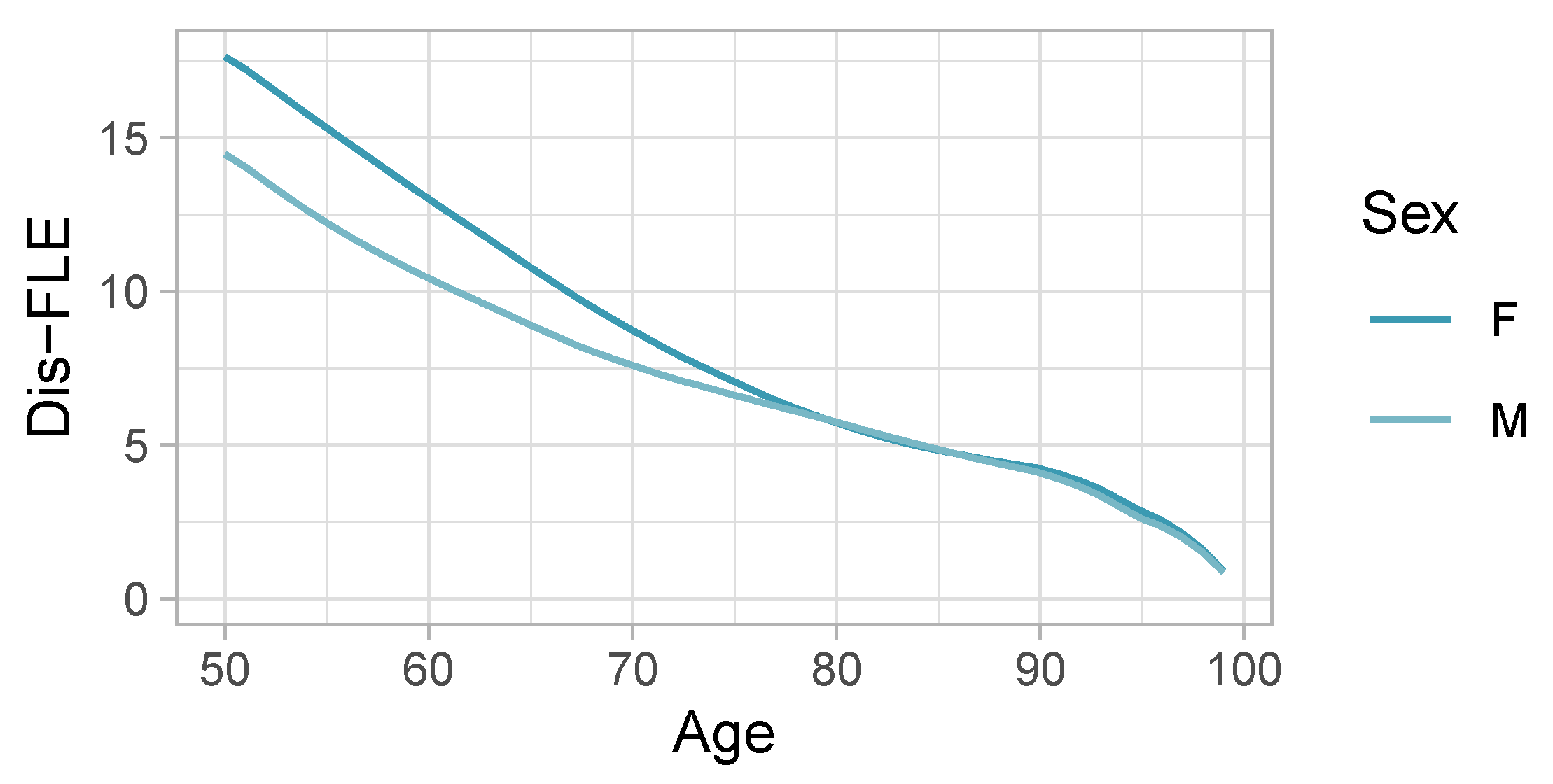
We estimated Dis-FLE using Kaplan–Meier survival curve estimates on the data adjusted for the whole population. The data allowed us to calculate the entire survival curve and Dis-FLE for each age. Figure 1 and Figure 2 show the survival curves and Dis-FLE with the adjustment for the whole population. Life duration in good health was significantly larger with than without the whole-population adjustment (see Figure A1 and Figure A2 in the Appendix B for the unadjusted curves).
Overall, Dis-FLE steadily decreased from 50 to about 80, before stabilizing from about 80 to 90 and continuing to decrease thereafter. Seeing the entire curve revealed an interesting pattern: the sex gap between Dis-FLE started at about 5 years at 50, and decreased to 0 at 80. Dis-FLE for men and women stayed essentially the same thereafter. Dis-FLE without the whole-population adjustment (Figure A2 in the Appendix B) did display a proportionally consistent sex gap; therefore, the closing of the sex gap observed in Figure 2 was due to the whole-population adjustment. There was a higher proportion of men than women who never entered a hospital. Therefore, the adjustment added more healthy men than healthy women, thus having a favorable impact on Dis-FLE for men relative to women. However, this observation is difficult to interpret and requires further investigation in future research. For this reason, we focused on the Cox model for the hospitalized population only.
To place the proposed Dis-FLE indicator into context of existing health indicators, we compared it to the closest available indicator, Eurostat’s Healthy Life Years (HLY) for France over the same period (Eurostat 2020). HLY’s concept of health is based on a self-evaluation of long-term activity limitation, as measured by GALI of the EU-SILC survey.
HLY represents the expected life duration without long-term activity limitation. This indicator was deliberately chosen to reflect the overall level of perceived ability, without attempting to identify the source or type of limitations. This allows it to be simple and be widely applied, thus increasing coverage and allowing for comparisons between countries and over time (Robine 2003).
HLY is also the only comparable health indicator covering France in the observation period. Another candidate was the HALE indicator from the Global Burden of Disease study for France, but it is not directly comparable to Dis-FLE-type indicators, as HALE assigns weights to different health states. Finally, previous articles using these data (Guibert et al. 2018a, 2018b) focused on similar Dis-FLE-type indicator, but they took into consideration only a small number of severe diseases, resulting in significantly longer Dis-FLE.
Table 6 compares Dis-FLE adjusted for the whole French population with HLY at ages 50 and 65. In general, Dis-FLE and HLY followed expected patterns, decreasing from age 50 to 65 for both genders. Women consistently exhibited higher Dis-FLE and HLY compared to men across all ages. However, at age 50, Dis-FLE was significantly lower than HLY for both genders. Furthermore, the sex gap was more pronounced in Dis-FLE. At 50, for Dis-FLE, the female–male gap was 2 years larger than for HLY. At 65, the difference between sexes was smaller but still present at about 1 year.
Assuming that the Dis-FLE estimates are indeed representative of the general population, then the difference may be explained by the difference of perceived activity limitation as measured by GALI and their clinical state, as well as the exclusion of institutional households in the EU-SILC survey.

4.2. Cox Model Inferences

In this section, we analyze the data through the Cox model described in Section 3. This model allows us to identify factors influencing health. Through this analysis, we illustrate the advantages of using clinical data. A similar analysis would not be possible with other data sources, either because they lack the necessary information (covariables) or volume.
We present hazard ratios estimated for this Cox model, that is, e β j for the j th variable, rather than the model coefficient, β j . For non-age-dependent effects, we give the numeric value of the ratio in a table. For terms with age-dependent effects, we show curves of ratios as a function of age.
Overall, the available covariables had a large impact on healthy life duration, with behavioral risk factors having the largest impact, but that impact also decreased with age. Following the risk factors, sex was important, with men experiencing adverse events earlier than women, even after controlling for covariables. As with the risk factors, the difference became smaller for later ages.
In the following sections, we examine one-by-one the effects of the risk factors, but first, we want to get an overall idea of just how much the risk factors influence Dis-FLE.
N.B.: the estimates of Dis-FLE and other quantities do not represent estimates for the general French population as the adjustment described in Section 3.3 cannot be applied for the Cox model.

4.2.1. Risk Profiles

Before delving into the individual impact of each variable, we first illustrate the collective discriminatory power of the model by examining survival curves and Dis-FLE for selected risk profiles. As is seen later in this section, the presence of risk-increasing behaviors (smoking, obesity, and alcohol consumption) is the determinant factor of Dis-FLE. Therefore, the risk profiles are simply the number of risk-increasing behaviors present (smoking, obesity, and alcohol consumption):
  • The “Lowest” risk profile, representing individuals without any risk factors.
  • The “Intermediate” risk profile, involving one risk-increasing behavior.
  • The “Highest” risk profile, featuring two risk-increasing behaviors.
Figure 3 and Figure 4 display survival curves and Dis - FLE ( t ) estimated by the Cox model for these risk profiles. There are two curves for the “Lowest” risk profile, one for men and one for women, while the “Intermediate” and “Highest” profiles each include six curves, one for each combination of sex and one of the risk factors. Since these risk profiles are just groupings of covariables, they remain constant for each individual.
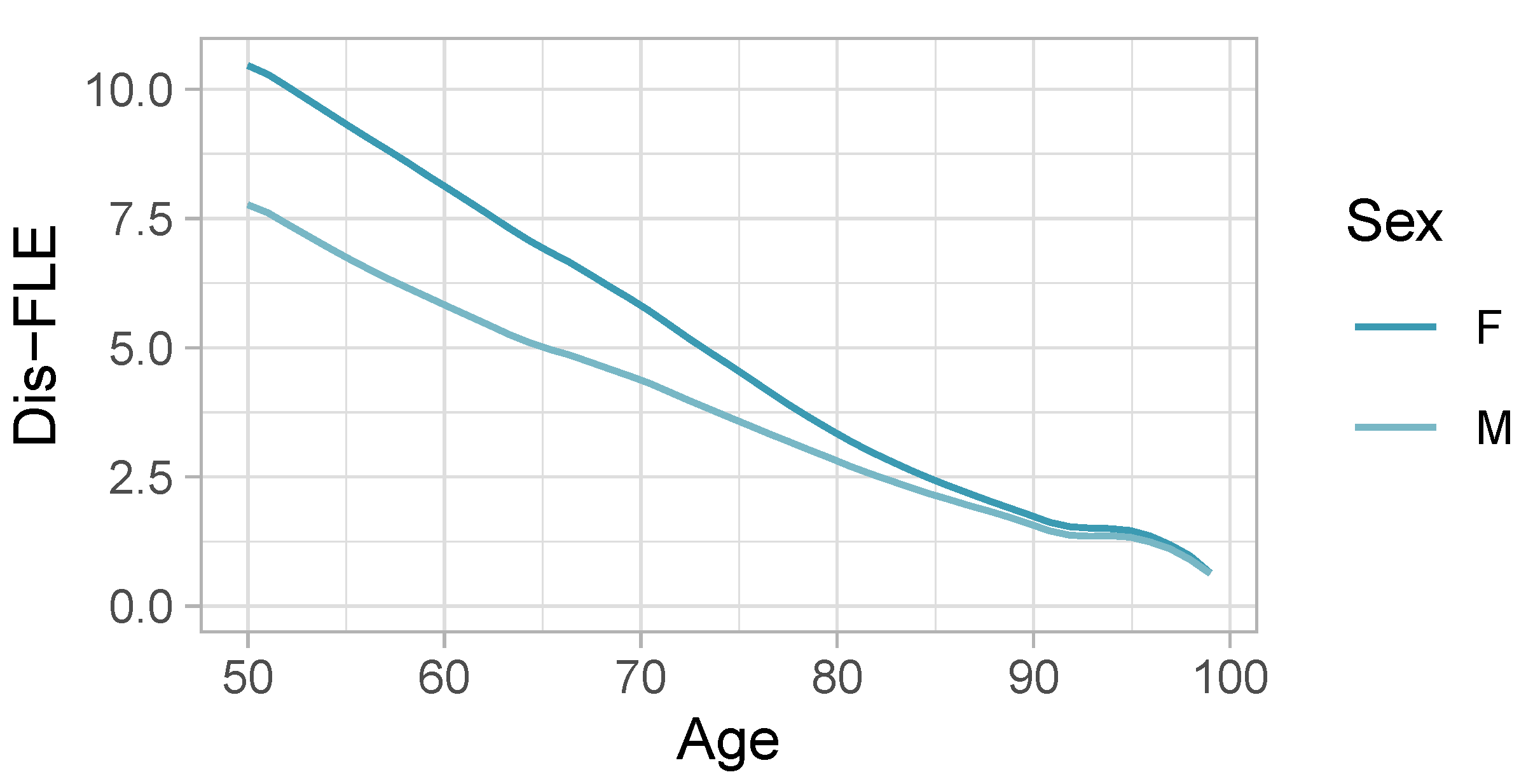
The impact of risk behaviors on disease-free life duration was evident, with a substantial 10-year range in Dis-FLE at age 50 between the lowest and highest risk profiles. Having at least one risk-increasing behavior appeared to be a key factor, reducing Dis-FLE by approximately 5 years. In the absence of such behaviors, sex emerged as the determining factor for Dis-FLE.
It is worth noting that Dis-FLE curves may intersect for men and women in some risk profiles due to age-dependent coefficients in the Cox model. Additionally, these figures allowed us to isolate the sex gap when other factors were equal. For instance, in the absence of risk factors at age 50, the sex gap was approximately 2.5 years. However, with the presence of at least one risk factor, this gap diminished to less than a year. This indicates that while behavioral differences contribute to the Dis-FLE sex gap, they do not entirely explain it.

4.2.2. Sex

We now proceed to inspect the effect of each variable on the disease-free life duration one by one. We examine age-dependent hazard ratios. The first variable analyzed was the sex of the individual. To take into account the apparent non-proportionality of hazard functions, the estimated hazard ratio of sex was allowed to vary with age and was modeled by a step function. All else being equal, men had a larger hazard than women, even when controlling for other covariates, as seen in Figure 5. This difference was not constant over time; it started off at about 30% excess hazard at 50, and rose steadily before attaining a maximum of almost 45% excess hazard at about 70 years of age. The difference then declined to 5% at 100 years.
Note that Figure 4 illustrates the impact of sex on Dis-FLE while keeping other variables constant. From it, we see that in the absence of risk factors, Dis-FLE was 2.5 years lower for men than for women. In the presence of at least one risk factor, the difference was less than a year.

4.2.3. Behavioral Risk Factors

We analyzed the effect of three risk factors:
  • Tobacco consumption;
  • Alcohol consumption;
  • Obesity.
Each risk factor was grouped into three risk categories, 0, 1, and 2. Category 0 represented the absence of risk-increasing behavior and was taken as reference. Figure 6 shows the age-dependent effects for these risk factors. All risk factors appeared to have a large negative impact on the outcome. The impact of these risk factors appeared to decrease with age.
Category 2 alcohol abuse had the largest impact on health (although it also impacted the smallest population compared to other risk factors), followed by smoking and obesity. The hazard ratios for category 1 risk factors were substantially smaller. All hazard ratios decreased with age.

4.2.4. Multiple Behavioral Risk Factors

In our analysis, we investigated the combined impact of multiple risk factors. Given the extensive range of possible combinations involving category 1 and 2 risk factors, we specifically concentrated on the most prevalent interactions—those among category 2 risk factors.
We found that multiple risk factors increased the overall risk. However, the marginal increase in risk was less pronounced compared to the risk associated with each factor independently. This suggested a compensatory effect when multiple behavioral risk factors coexisted. Notably, the combination of alcohol and smoking exhibited the highest compensatory ratio, followed by obesity–alcohol and obesity–smoking.
Figure 7 visually represents the distinctions between:
  • The main effects;
  • The naive combined effect of two risk factors (calculated by multiplying the hazard ratios of the main effects without considering the interaction term);
  • The estimated effect that accounts for the interaction term.
For all three combinations of risk factors, the combined effect with interaction was lower than without it. These observations shed light on the nuanced interplay of risk factors and their collective influence on the overall hazard.

4.2.5. Behavioral Risk Factors Conditional on Sex

We measured whether risk factors impacted men and women differently. To simplify the model, we modeled this difference as an offset for males. Table 7 gives the hazard ratios for the interaction terms between sex and behavioral risk factors. These ratios can be interpreted as additional burden of these risk factors on men, relative to women.
Overall men appeared to be slightly less sensitive to the presence of behavioral risk factors. This explains in part the reason for the decrease in the Dis-FLE sex gap in the presence of risk factors, as seen in Figure 4.
We focused on category 2 behavioral risk factors because category 1 ones were rare or without substantial male–female differences. Category 2 alcohol consumption had a substantially stronger impact on women, with women suffering an additional 12% of hazard. Obesity also impacted women stronger, by about 7%, while men’s health was slightly more sensitive to smoking.

4.2.6. Geographical

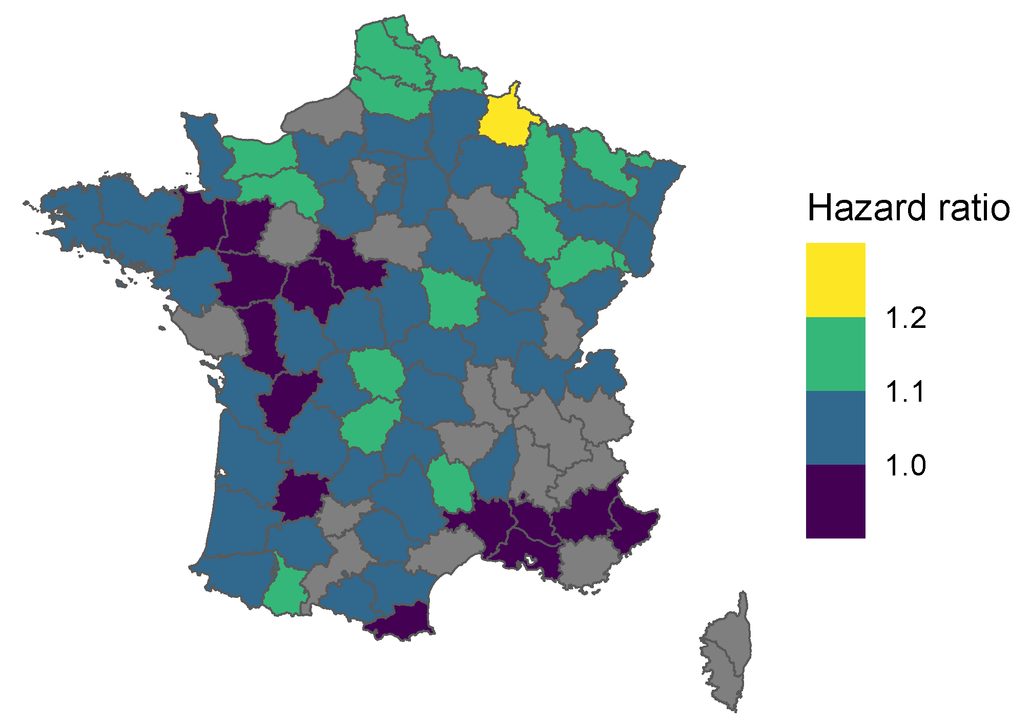
Figure 8 gives the hazard ratios relative to the Yvelines department (78). This reference was chosen because it is in the Île-de-France region, while not being Paris itself.
Northern departments had a markedly higher hazard rate, even after controlling for other covariates. South-east and eastern departments, on the other hand, appeared to have the inverse effect. Both these facts are in accord with the previous literature. In the rest of the territory, the effects appeared to be more local.
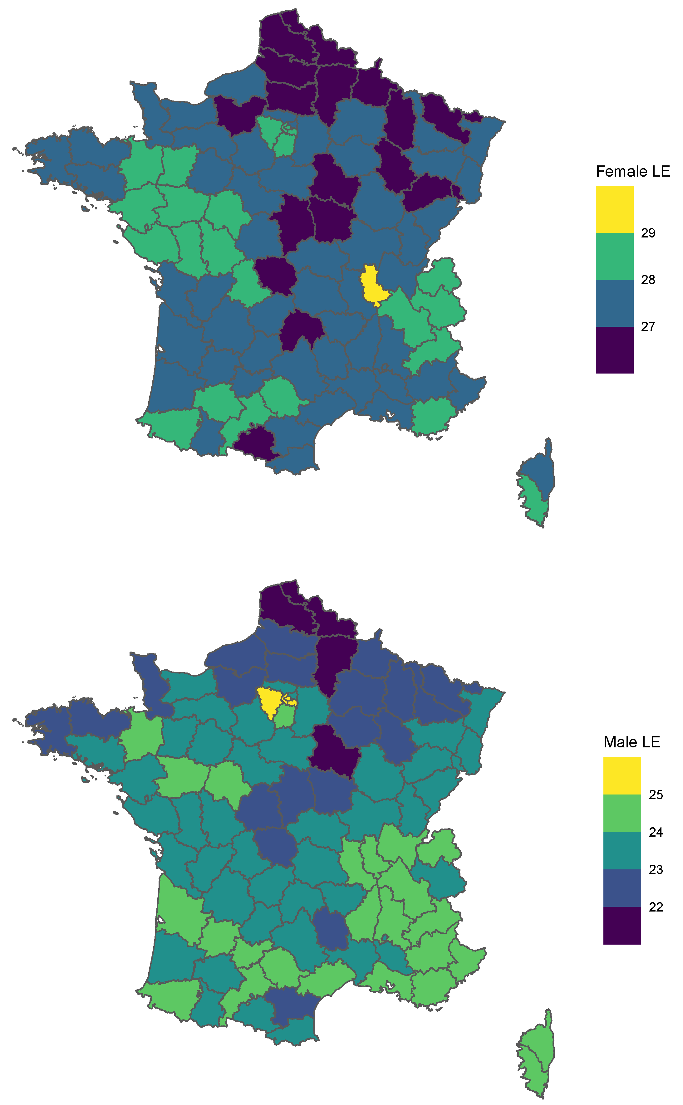
To put these results in context, Figure 9 provides a map of life expectancy at 60 by sex and by department. Overall, we observe similar trends. The similarity suggests that the geographic location is an independent predictor of life expectancy and Dis-FLE.
In and of itself, it is hard to interpret this result, as it may not necessarily reflect the impact of local environment on health, but instead reflect the level of access to healthcare, as discussed when introducing this approach. Further work is necessary to explain these differences. A first step would be including more information on the departments themselves, e.g., population, population density, GDP, median income, etc.
The variables “Education” and “Immigration” indicate the level of education and immigration in the commune of residence. Table 8 gives the obtained hazard ratios for these variables. Surprisingly, the level of education and immigration in the commune of residence appeared to increase the hazard. The effect was minor compared to other risk factors, but nonetheless significant. This result is also hard to interpret on it own as there is a level of indirection between the individual and the commune of residence.

5. Conclusions

We proposed the use of clinical data to construct health indicators. The use of clinical data opens up a hitherto unused source of information and makes a rich analysis possible, some of which we present in this paper.
This work provides a methodological blueprint for calculating health indicators based on clinical datasets. The implications of our research extend beyond the French context, with potential applications in other countries and healthcare systems. Specifically, our methodology is not confined to large clinical datasets and can be applied at smaller scales, such as hospital cohorts, in France or elsewhere. However, when considering entire populations, accessing national hospitalization datasets to calculate nationally representative health indicators can be exceedingly challenging. We hope that this work provides a precedent that will encourage and facilitate similar efforts in the future.
Although clinical data impose a diagnosis-centric vision rather than an outcome-based one that may be provided by health-oriented survey instruments, it does provide a clear outline of the health state over the lifetime of the patient. When combined with the large volume of data available, this results in pertinent indicators on a population level. Indeed, as the comparison with HLY shows, Dis-FLE with the adjustment for the whole population displays similar trends, although with a wider sex gap.
In the absence of standardized practice to define health from clinical data, it is difficult to construct comparable health indicators. We sidestepped the issue by focusing on a simple definition of being disease-free. A more complex indicator would take into account the entire health trajectory but would be difficult to analyze; this could be addressed in further work. Instead, our focus on simple trajectories combined with a large volume of data available allowed us to exhaustively analyze the impact of available covariables. In doing so, we illustrated the kind of analysis we believe can be made possible by using clinical data. We applied the proposed methods to the French PMSI database and analyzed the health status of the population aged 50 and up from 2010 to 2013. We summarized the results of the analysis in terms of Dis-FLE based on 36 severe conditions and hazard ratios of the corresponding Cox model.
For the population studied, the Dis-FLE at 50 years was 10 years for women and 7.5 for men. Dis-FLE was strongly influenced by the covariables available; indeed Dis-FLE ranged from 2.5 to 12.5 for women and from 2.5 to 10 for men when conditioned on covariates.
The most important determinants of Dis-FLE were the behavioral factors; in order of importance: alcohol consumption, tobacco use, and obesity. Each of these had hazard ratios exceeding two for all ages before 80. Alcohol consumption had a hazard ratio larger than three before 60 years. Interestingly, all age-dependent effects decreased with age after 60.
Sex also had a large influence with a hazard ratio above 1.2 before 80 and as large as 1.4 at about 70. Also, the effect of behavioral risk factors was found to differ by sex, with alcohol consumption and obesity having a stronger effect on women, and smoking having a stronger effect on men. Other factors influenced Dis-FLE, but have a weaker effect.
The Cox model analyzed in this paper was the simplest model that still allowed us to illustrate the richness of the underlying data. There are, however, many possible improvements to it. For example, the model analyzed did not take into account calendar time. This is in contrast to most indicators where the ability to follow them over time is vital. A natural extension of the model would be to take into account calendar time by including it as an age-dependent covariate. Another possible extension includes making effects not only depend on age but also on calendar time, therefore modeling possible improvements form the treatment of behavioral factors.
The trajectories analyzed were based on a specific definition of health or more specifically of the disease-free concept. This definition was based on previous work using this dataset and was conceptually coherent with other indicators. However, it lacks direct comparable indicators, making its usefulness as an indicator limited for now. Further work may help identify a definition of disability more closely aligned with other indicators, such as GALI.
More fundamentally, the concept of health used introduces an artificial dichotomy between good and ill health. Using the same data, it should be possible to define more realistic individual trajectories, for example, by assigning each disease a weight. Using this approach, we could define individual-level health-weighted indicator, extending the flexible approach to other indicators such as HALE. In this context, the use of clinical data would also simply be a methodology issue, as many problems plaguing HALE estimates are resolved by these data, for example, comorbidity and the nuance between incidence and prevalence.
Such an approach would make both the definition of health trajectories and their analysis significantly more complex. However, we believe that it would be a natural next step in using clinical data as data source for health indicators.
Beyond considerations of the health concept used, the use of clinical data requires additional assumptions and adjustment procedures to produce nationally representative indicators. A simple adjustment procedure was introduced and used to calculate Dis-FLE for the general French population. However, we believe that this procedure could be improved by using more granular data and under additional assumptions, extended to the estimates provided by the Cox model.
Should our methodology and findings prove useful and robust, future work could delve into the development of a definition of health, that is based on clinical data that explicitly target GALI or other relevant health indicators, potentially drawing upon detailed assessments of activities of daily living (ADLs). Such an endeavor could enhance the accuracy and sensitivity of our understanding of disability and its implications for individual and population health.
The Cox model was the tool of choice for this analysis. However, the large volume of data combined with the need to explicitly define the model matrix required a large amount of computer memory to do the necessary computations. The use of other machine learning algorithms may provide a more efficient means to analyze this dataset.

Author Contributions

Conceptualization, O.S., Q.G., and F.P.; data curation, M.S. and Q.G.; methodology, O.S., Q.G., and F.P.; software, O.S.; writing—original draft, O.S.; writing—review and editing, Q.G., F.P., and M.S. All authors have read and agreed to the published version of the manuscript.

Funding

This research received no external funding.

Institutional Review Board Statement

Not applicable.

Informed Consent Statement

The requirement for informed consent was waived as data were deidentified.

Data Availability Statement

The data are not publicly accessible. The data used in this study can only be obtained from the Agence Technique de l’Information sur l’Hospitalisation (ATIH). The study was approved by the French National Commission for Data Protection (CNIL DE-2015-025), who granted access to the French National Hospital Discharge database for the years 2008 to 2013.

Acknowledgments

The authors are grateful to Christian Robert (ISFA—SAF Laboratory) for providing guidance on writing of this manuscript.

Conflicts of Interest

The authors declare no conflicts of interest.

Appendix A. Exclusion Criteria

Table A1 gives the exclusion criteria applied to the dataset.
Table A1. Exclusion criteria and impact on number of patients. Translated and adapted from Table 1 in (Schwarzinger 2018).
CriteriaYearsPop. Size% of Total Pop.
Hospitalized population, aged 50 and up2008–201318,440,022100.0%
Exclusion criterion 1: severe conditions under study observed in 2008–20092008, 20094,730,65125.7%
Alzheimer’s disease 508,5752.8%
Other severe conditions 4,554,01024.7%
Total loss of autonomy, cognitive or physical 205,6811.1%
Death observed in a hospital 572 4543.1%
Death outside of hospital (imputed from other data) 272 7421.5%
Exclusion criterion 2: other conditions not covered by dependence insurance 914,5955.0%
Major neurological disorder2008, 2009
Paralysis 197,0961.1%
Coma 97,4760.5%
Transplant recipients (of an organ or of bone marrow)2008, 200936,5930.2%
Birth defects and genetic disorders2008–2013
Birth defect or chromosome abnormality (including trisomy 21) 272,8871.5%
Primary immunodeficiency 37,1010.2%
Thalassemia, sickle cell disease, and other blood disorders 16,2000.1%
Hemophilia and other bleeding disorders 16,6000.1%
Inborn errors of metabolism (including hemochromatosis and cystic fibrosis) 210,1761.1%
Cerebral palsy and genetic neuromuscular disorders (including myopathy) 70,5870.4%
Other genetic disorders (including Alport syndrome) 22520.0%
Infections2008–2013
Human immunodeficiency viruses (HIV) 43,7340.2%
Infectious diseases (including tuberculosis and encephalitis) 49,5240.3%
Mental disorders2008–2013
Schizophrenia and others delusional disorders 175,5271.0%
Intellectual disability 44,9360.2%
Hospitalized population, aged 50 and up in good health on the 1st of January 2010 (selected after exclusion criteria 1 and 2)2010–201313,170,35571.4%
Data preparation for analysis2008, 20092,559,72613.9%
Censored before 1 January 2010 2,012,81510.9%
End of observation period ends before 50 896,1114.9%
Population included in study2010–201310,610,62957.5%

Appendix B. Sex-Specific Survival Curves without Adjustment
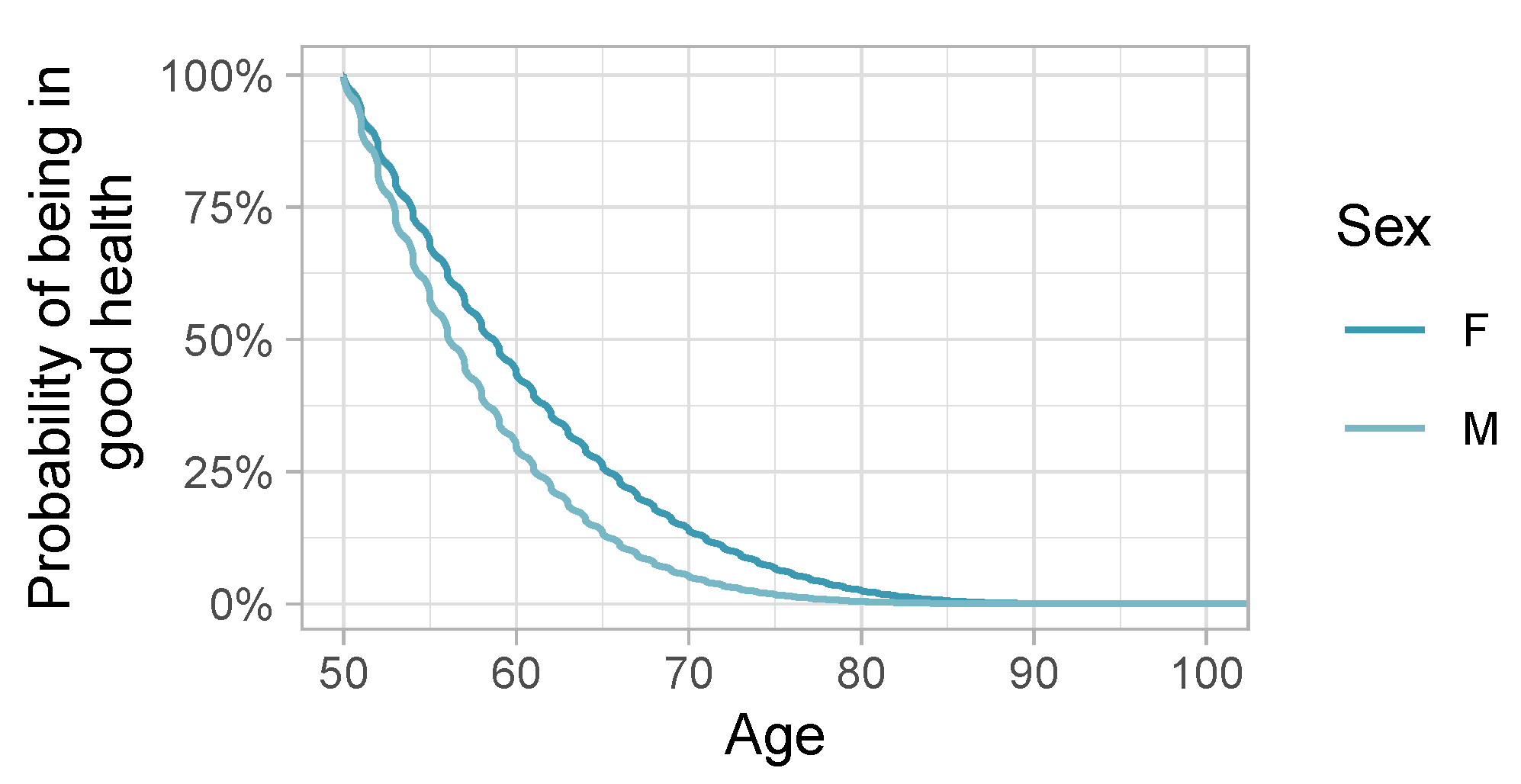
Figure A1 shows the sex-specific survival curves without adjustment for the whole population. Unsurprisingly women spent longer in a healthy state than men. The oscillations in the curves are due to rounding in anonymized dates. Figure A2 shows the corresponding Dis - FLE ( t ) .
Figure A1. Survival curves of being in good health, by sex.
Risks 12 00092 g0a1
Figure A2. Conditional Dis-FLE as a function of age and sex.
Risks 12 00092 g0a2

Appendix C. Model Diagnostics

The cox model used was fit on 60% of the available data. The remaining 40% were reserved to perform model diagnostics presented in this section.
The C-statistic calculated on the test set was 59.91%.
To evaluate the quality of the fit on the test dataset, we calculated the linear predictor, i.e., log ( Hazard ratio ) , for every individual. Individuals were then classified into classes based on the calculated value. The distribution of linear predictors was clustered around few values. This is due to the fact that the influence of sex and the presence of risk factors essentially determined the risk, with all other variables essentially only adding noise. The lowest interval, ( , 0.2 ] , essentially covered only women without any risk factors; ( 0.2 , 0.7 ] covered men without any risk factors; ( 0.7 , 1.1 ] covered mostly persons with obesity; ( 1.1 , 1.5 ] covers mostly smokers; and ( 1.5 , ] covered persons with alcohol consumption, or multiple risk factors. Finally, Figure A3 compares the observed survival curves for each of these classes with the predicted survival curve.
One problem with this approach is that the model includes age-dependent coefficients. This means that the risk score for each individual changes over time, making it impossible to attribute a constant score to each individual. However, since the observation period was four years and the time grid for age-dependent coefficient was two years, each individual could at most have three unique risk values, and most had only one. When multiple risk values were present, they were close to each other. For the calculation above, we used the average of the predicted linear prediction scores.
Figure A3. Comparison between observed and estimated survival functions for the test dataset, grouped by linear predictor.
Risks 12 00092 g0a3

Appendix D. All Cox Model Coefficients

Table A2. All Cox model coefficients with associated standard errors and p-values.
TermHazard RatioStd. Err.p-Value
Obesity, cat. 11.620.010.00
Obesity, cat. 22.200.020.00
Alcohol, cat. 11.240.030.00
Alcohol, cat. 23.300.010.00
Smoking, cat. 12.250.040.00
Smoking, cat. 22.500.010.00
Sex: M1.280.010.00
Department of residence: 021.070.010.00
Department of residence: 031.050.010.00
Department of residence: 040.950.010.00
Department of residence: 051.020.020.16
Department of residence: 060.910.010.00
Department of residence: 071.030.010.01
Department of residence: 081.200.010.00
Department of residence: 091.060.010.00
Department of residence: 101.000.010.83
Department of residence: 111.070.010.00
Department of residence: 121.040.010.00
Department of residence: 130.950.010.00
Department of residence: 141.090.010.00
Department of residence: 151.030.010.02
Department of residence: 160.960.010.00
Department of residence: 171.060.010.00
Department of residence: 181.080.010.00
Department of residence: 191.100.010.00
Department of residence: 211.030.010.00
Department of residence: 221.080.010.00
Department of residence: 231.090.010.00
Department of residence: 241.050.010.00
Department of residence: 251.060.010.00
Department of residence: 261.010.010.59
Department of residence: 271.040.010.00
Department of residence: 281.040.010.00
Department of residence: 291.030.010.00
Department of residence: 2A1.030.010.06
Department of residence: 2B0.990.010.46
Department of residence: 300.980.010.01
Department of residence: 311.010.010.33
Department of residence: 321.060.010.00
Department of residence: 331.020.010.04
Department of residence: 341.000.010.97
Department of residence: 350.980.010.05
Department of residence: 361.030.010.01
Department of residence: 370.980.010.05
Department of residence: 381.000.010.64
Department of residence: 391.020.010.14
Department of residence: 401.030.010.01
Department of residence: 410.980.010.04
Department of residence: 420.980.010.06
Department of residence: 431.010.010.27
Department of residence: 441.030.010.00
Department of residence: 451.010.010.14
Department of residence: 461.040.010.00
Department of residence: 470.970.010.00
Department of residence: 481.110.020.00
Department of residence: 490.940.010.00
Department of residence: 501.070.010.00
Department of residence: 511.030.010.00
Department of residence: 521.130.010.00
Department of residence: 530.930.010.00
Department of residence: 541.050.010.00
Department of residence: 551.130.010.00
Department of residence: 561.070.010.00
Department of residence: 571.140.010.00
Department of residence: 581.100.010.00
Department of residence: 591.100.010.00
Department of residence: 601.040.010.00
Department of residence: 611.090.010.00
Department of residence: 621.120.010.00
Department of residence: 631.080.010.00
Department of residence: 641.080.010.00
Department of residence: 651.090.010.00
Department of residence: 660.960.010.00
Department of residence: 671.050.010.00
Department of residence: 681.040.010.00
Department of residence: 691.020.010.06
Department of residence: 701.090.010.00
Department of residence: 711.020.010.02
Department of residence: 721.000.010.86
Department of residence: 731.020.010.07
Department of residence: 741.020.010.02
Department of residence: 751.030.010.00
Department of residence: 761.010.010.11
Department of residence: 771.050.010.00
Department of residence: 780.980.010.08
Department of residence: 790.960.010.00
Department of residence: 801.080.010.00
Department of residence: 811.060.010.00
Department of residence: 820.980.010.05
Department of residence: 830.990.010.20
Department of residence: 840.940.010.00
Department of residence: 851.000.010.91
Department of residence: 861.030.010.00
Department of residence: 871.070.010.00
Department of residence: 881.030.010.00
Department of residence: 891.070.010.00
Department of residence: 901.090.020.00
Department of residence: 911.020.010.01
Department of residence: 921.030.010.00
Department of residence: 931.070.010.00
Department of residence: 941.040.010.00
Department of residence: 951.040.010.00
Immigration: Q11.000.000.25
Immigration: Q21.010.000.00
Immigration: Q31.010.000.00
Education: Q11.030.000.00
Education: Q21.050.000.00
Education: Q31.070.000.00
Obesity, cat. 1 × Alcohol, cat. 10.840.030.00
Obesity, cat. 2 × alcohol, cat. 10.880.060.03
Obesity, cat. 1 × alcohol, cat. 20.760.010.00
Obesity, cat. 2 × alcohol, cat. 20.690.020.00
Obesity, cat. 1 × smoking, cat. 10.680.020.00
Obesity, cat. 2 × smoking, cat. 10.640.050.00
Obesity, cat. 1 × smoking, cat. 20.770.010.00
Obesity, cat. 2 × smoking, cat. 20.750.010.00
Obesity, cat. 1 × sex: M0.980.000.00
Obesity, cat. 2 × sex: M0.930.010.00
Alcohol, cat. 1 × smoking, cat. 10.780.040.00
Alcohol, cat. 2 × smoking, cat. 10.530.030.00
Alcohol, cat. 1 × smoking, cat. 20.670.020.00
Alcohol, cat. 2 × smoking, cat. 20.600.010.00
Alcohol, cat. 1 × sex: M1.010.020.63
Alcohol, cat. 2 × sex: M0.880.010.00
Smoking, cat. 1 × sex: M0.920.020.00
Smoking, cat. 2 × sex: M1.010.000.02
Obesity, cat. 1 × spline (age): knot 11.010.010.48
Obesity, cat. 2 × spline (age): knot 11.020.030.46
Obesity, cat. 1 × spline (age): knot 21.010.010.49
Obesity, cat. 2 × spline (age): knot 21.020.030.34
Obesity, cat. 1 × spline (age): knot 31.030.010.05
Obesity, cat. 2 × spline (age): knot 31.040.030.12
Obesity, cat. 1 × spline (age): knot 41.030.010.02
Obesity, cat. 2 × spline (age): knot 41.030.020.25
Obesity, cat. 1 × spline (age): knot 51.030.010.05
Obesity, cat. 2 × spline (age): knot 51.030.030.19
Obesity, cat. 1 × spline (age): knot 61.010.010.66
Obesity, cat. 2 × spline (age): knot 61.020.030.35
Obesity, cat. 1 × spline (age): knot 70.940.010.00
Obesity, cat. 2 × spline (age): knot 70.880.030.00
Obesity, cat. 1 × spline (age): knot 80.700.050.00
Obesity, cat. 2 × spline (age): knot 80.580.160.00
Alcohol, cat. 1 × spline (age): knot 11.010.030.76
Alcohol, cat. 2 × spline (age): knot 11.020.010.25
Alcohol, cat. 1 × spline (age): knot 21.040.030.18
Alcohol, cat. 2 × spline (age): knot 20.980.010.10
Alcohol, cat. 1 × spline (age): knot 31.150.040.00
Alcohol, cat. 2 × spline (age): knot 30.940.020.00
Alcohol, cat. 1 × spline (age): knot 41.130.040.00
Alcohol, cat. 2 × spline (age): knot 40.910.010.00
Alcohol, cat. 1 × spline (age): knot 51.160.040.00
Alcohol, cat. 2 × spline (age): knot 50.840.020.00
Alcohol, cat. 1 × spline (age): knot 61.210.050.00
Alcohol, cat. 2 × spline (age): knot 60.790.020.00
Alcohol, cat. 1 × spline (age): knot 71.110.050.03
Alcohol, cat. 2 × spline (age): knot 70.680.020.00
Alcohol, cat. 1 × spline (age): knot 80.740.410.47
Alcohol, cat. 2 × spline (age): knot 80.290.100.00
Smoking, cat. 1 × spline (age): knot 11.070.050.14
Smoking, cat. 2 × spline (age): knot 11.020.010.11
Smoking, cat. 1 × spline (age): knot 21.060.050.20
Smoking, cat. 2 × spline (age): knot 21.020.010.03
Smoking, cat. 1 × spline (age): knot 31.020.050.60
Smoking, cat. 2 × spline (age): knot 31.000.010.96
Smoking, cat. 1 × spline (age): knot 40.950.050.28
Smoking, cat. 2 × spline (age): knot 40.950.010.00
Smoking, cat. 1 × spline (age): knot 50.860.050.00
Smoking, cat. 2 × spline (age): knot 50.870.010.00
Smoking, cat. 1 × spline (age): knot 60.790.050.00
Smoking, cat. 2 × spline (age): knot 60.830.010.00
Smoking, cat. 1 × spline (age): knot 70.690.050.00
Smoking, cat. 2 × spline (age): knot 70.700.010.00
Smoking, cat. 1 × spline (age): knot 80.440.260.00
Smoking, cat. 2 × spline (age): knot 80.440.030.00
Sex: M × spline (age): knot 11.020.010.01
Sex: M × spline (age): knot 21.070.010.00
Sex: M × spline (age): knot 31.100.010.00
Sex: M × spline (age): knot 41.120.010.00
Sex: M × spline (age): knot 51.100.010.00
Sex: M × spline (age): knot 61.050.010.00
Sex: M × spline (age): knot 70.940.010.00
Sex: M × spline (age): knot 80.840.020.00

References

  1. Abe, Shinzo. 2013. Japan’s strategy for global health diplomacy: Why it matters. The Lancet 382: 915–16. [Google Scholar] [CrossRef] [PubMed]
  2. Bogaert, Petronille, Herman Van Oyen, Isabelle Beluche, Emmanuelle Cambois, and Jean-Marie Robine. 2018. The use of the global activity limitation Indicator and healthy life years by member states and the European Commission. Archives of Public Health 76: 30. [Google Scholar] [CrossRef] [PubMed]
  3. Euro-REVES, Carol Jagger, Viviana Egidi, and Jean Marie Robine. 2000. Selection of a Coherent Set of Health Indicators. Final Draft, Euro-REVES. Available online: https://ec.europa.eu/health/ph_projects/1998/monitoring/fp_monitoring_1998_frep_03_en.pdf (accessed on 16 June 2023).
  4. Eurostat. 2020. Healthy Life Years by Sex (from 2004 Onwards) (hlth_hlye). Eurostat Database. Available online: https://ec.europa.eu/eurostat/databrowser/view/HLTH_HLYE/default/table?lang=en (accessed on 16 May 2023).
  5. Fries, James F. 1980. Aging, Natural Death, and the Compression of Morbidity. New England Journal of Medicine 303: 130–35. [Google Scholar] [CrossRef] [PubMed]
  6. Gruenberg, Ernest M. 2005. The Failures of Success. Milbank Quarterly 83: 779–800. [Google Scholar] [CrossRef] [PubMed]
  7. Guibert, Quentin, Frédéric Planchet, and Michaël Schwarzinger. 2018a. Mesure de l’espérance de vie sans dépendance totale en France métropolitaine. Bulletin Français d’Actuariat 18: 85–109. [Google Scholar]
  8. Guibert, Quentin, Frédéric Planchet, and Michaël Schwarzinger. 2018b. Mesure du risque de perte d’autonomie totale en France métropolitaine. Bulletin Français d’Actuariat 18: 133–59. [Google Scholar]
  9. Head, Jenny, Holendro Singh Chungkham, Martin Hyde, Paola Zaninotto, Kristina Alexanderson, Sari Stenholm, Paula Salo, Mika Kivimäki, Marcel Goldberg, Marie Zins, and et al. 2019. Socioeconomic differences in healthy and disease-free life expectancy between ages 50 and 75: A multi-cohort study. European Journal of Public Health 29: 267–72. [Google Scholar] [CrossRef] [PubMed]
  10. INSEE. 2022. La situation démographique en 2020. INSEE Reports. Available online: https://www.insee.fr/fr/statistiques/6327226?sommaire=6327254 (accessed on 15 May 2023).
  11. INSEE. 2023. Espérances de vie à différents âges. INSEE Reports. Available online: https://www.insee.fr/fr/outil-interactif/6794598/EVDA/DEPARTMENTS (accessed on 19 April 2024).
  12. Jagger, Carol, Eileen M. Crimmins, Yasuhiko Saito, Renata Tiene De Carvalho Yokota, Herman Van Oyen, and Jean-Marie Robine, eds. 2020. International Handbook of Health Expectancies. Volume 9 of International Handbooks of Population. Cham: Springer International Publishing. [Google Scholar] [CrossRef]
  13. Kempen, Gertrudis I. J. M., Nardi Steverink, Johan Ormel, and Dorly J. H. Deeg. 1996. The Assessment of ADL among Frail Elderly in an Interview Survey: Self-Report versus Performance-Based Tests and Determinants of Discrepancies. The Journals of Gerontology Series B: Psychological Sciences and Social Sciences 51B: P254–P260. [Google Scholar] [CrossRef] [PubMed]
  14. Kim, Young-Eun, Yoon-Sun Jung, Minsu Ock, and Seok-Jun Yoon. 2022. A Review of the Types and Characteristics of Healthy Life Expectancy and Methodological Issues. Journal of Preventive Medicine and Public Health 55: 1–9. [Google Scholar] [CrossRef] [PubMed]
  15. Klein, John P., Hans C. Van Houwelingen, Joseph G. Ibrahim, and Thomas H. Scheike, eds. 2016. Handbook of Survival Analysis. Boca Raton: Chapman and Hall/CRC. [Google Scholar] [CrossRef]
  16. Krause, Neal M., and Gina M. Jay. 1994. What Do Global Self-Rated Health Items Measure? Medical Care 32: 930–42. [Google Scholar] [CrossRef] [PubMed]
  17. Lagström, Hanna, Sari Stenholm, Tasnime Akbaraly, Jaana Pentti, Jussi Vahtera, Mika Kivimäki, and Jenny Head. 2020. Diet quality as a predictor of cardiometabolic disease–free life expectancy: The Whitehall II cohort study. The American Journal of Clinical Nutrition 111: 787–94. [Google Scholar] [CrossRef] [PubMed]
  18. Martinussen, Torben, and Thomas H. Scheike. 2006. Dynamic Regression Models for Survival Data. Statistics for Biology and Health. New York: Springer. [Google Scholar]
  19. Peersman, Wim, Dirk Cambier, Jan De Maeseneer, and Sara Willems. 2012. Gender, educational and age differences in meanings that underlie global self-rated health. International Journal of Public Health 57: 513–23. [Google Scholar] [CrossRef] [PubMed]
  20. R Core Team. 2022. R: A Language and Environment for Statistical Computing. Vienna: R Foundation for Statistical Computing. [Google Scholar]
  21. Robine, Jean-Marie. 2003. Creating a coherent set of indicators to monitor health across Europe: The Euro-REVES 2 project. The European Journal of Public Health 13: 6–14. [Google Scholar] [CrossRef] [PubMed]
  22. Sanders, Barkev S. 1964. Measuring community health levels. American Journal of Public Health and the Nation’s Health 54: 1063–70. [Google Scholar] [CrossRef] [PubMed]
  23. Schwarzinger, Michaël. 2018. Etude QalyDays: Données source et retraitements pour l’étude du risque perte d’autonomie. Bulletin Français d’Actuariat 18: 57–81. [Google Scholar]
  24. Schwarzinger, Michaël, Bruce G. Pollock, Omer S. M. Hasan, Carole Dufouil, Jürgen Rehm, and QalyDays Study Group. 2018. Contribution of alcohol use disorders to the burden of dementia in France 2008–13: A nationwide retrospective cohort study. The Lancet Public Health 3: e124–e132. [Google Scholar] [CrossRef] [PubMed]
  25. Stenholm, Sari, Jenny Head, Ville Aalto, Mika Kivimäki, Ichiro Kawachi, Marie Zins, Marcel Goldberg, Loretta G. Platts, Paola Zaninotto, Linda L. Magnusson Hanson, and et al. 2017. Body mass index as a predictor of healthy and disease-free life expectancy between ages 50 and 75: A multicohort study. International Journal of Obesity 41: 769–75. [Google Scholar] [CrossRef] [PubMed]
  26. Therneau, Terry M. 2023. A Package for Survival Analysis in R. R Package Version 3.6-4. Available online: https://CRAN.R-project.org/package=survival (accessed on 1 January 2024).
  27. WHO. 2023. World Health Statistics: Monitoring Health for the SGDs, Sustainable Development Goals. Technical Report. Geneva: World Health Organization. [Google Scholar]
  28. World Health Organization. 2015. International Statistical Classification of Diseases and Related Health Problems. 10th Revision (Fifth edition). Technical Report. Geneva: World Health Organization. ISBN 9789241549165. [Google Scholar]
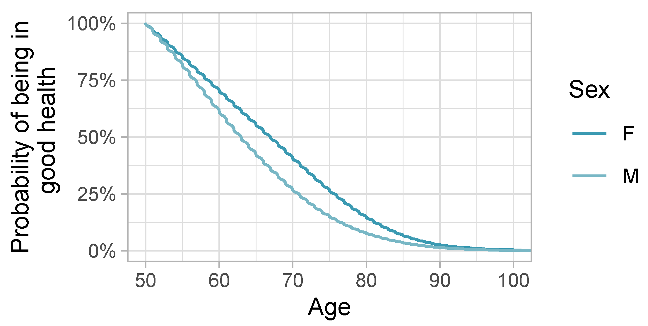
Figure 1. Survival curves of individuals without disease for the general population aged 50 and up, by sex.
Risks 12 00092 g001
Figure 2. Conditional Dis-FLE adjusted for the whole French population, aged 50 and up, as a function of age and sex.
Risks 12 00092 g002
Figure 3. Survival curves for selected risk profiles, by sex, with 95% confidence intervals.
Risks 12 00092 g003
Figure 4. Conditional residual expectation for selected risk profiles, by sex, with 95% confidence intervals.
Risks 12 00092 g004
Figure 5. Estimated age-dependent hazard ratio for sex. Values above 1 increase hazard for males. Gray areas are 95% pointwise confidence intervals.
Risks 12 00092 g005
Figure 6. Estimated age-dependent hazard ratios for behavioral risk factors. Values above 1 increase hazard. Gray areas are 95% pointwise confidence intervals.
Risks 12 00092 g006
Figure 7. Estimated age-dependent hazard ratios for two-way category 2 risk factors combinations. Each panel shows the interplay between two risk factors. For each panel, the main age-dependent effect is shown for the risk factors, and the combined effect with and without interaction are displayed. The combined effect without interaction is simply the product of the hazard ratios of the main effect. The combined effect with interactions is the product of the main effects and the interaction term. Values above 1 increase hazard. Gray areas are 95% pointwise confidence intervals.
Risks 12 00092 g007
Figure 8. Estimated hazard ratios for departments of residence. Values are binned. Values above 1 increase hazard relative to residents of department 78. Non-significant values (p-value > 0.05) are grayed out.
Risks 12 00092 g008
Figure 9. Life expectancy at 60, by sex, in France in 2023. Values are binned. Source: (INSEE 2023).
Risks 12 00092 g009
Table 1. Description of individual patient data.
ColumnPrecisionPossible ValuesDescription
IDIndividualPositive integersAnonymized identifier
AlcoholIndividual0, 1, 2Alcohol use disorder, grouped into three classes in increasing order: “0” for the absence of alcohol use disorder, “1” for mental and behavioral disorders due to former or current chronic harmful use of alcohol (ICD-10: F10.1–F10.9, Z50.2) including alcohol abstinence (ICD-10: F10.20–F10.23), “2” chronic diseases attributable to alcohol use disorders (e.g., Wernicke–Korsakoff syndrome, end-stage liver disease and other forms of liver cirrhosis, epilepsy, and head injury)
ObesityIndividual0, 1, 2Obesity, grouped into three classes in increasing order:
“0” body mass < 30 kg/m2,
“1” body mass ≥ 30 kg/m2 and <40 kg/m2,
“2” body mass > 40 kg/m2.
SmokerIndividual0, 1, 2Smoking, grouped into three classes in increasing order: “0”: no disorder due to tobacco use recorded, “1”: mental and behavioral disorders due to tobacco use (ICD-10: F17), “2”: mental and behavioral disorders due to tobacco use (ICD-10: F17) and Chronic Obstructive Pulmonary Disease (ICD-10: J44.9).
DepartmentIndividual“01” to “96”Department of residence (Metropolitan France)
Immigrationpostal code0, 1, 2, 3Proportion of foreign nationals, grouped into quartiles, proxy for immigration status
Educationpostal-code0, 1, 2, 3Proportion of population with higher education, grouped into quartiles, proxy for education
SexIndividual“M” or “F”M: male, F: female
Year of birthIndividualintegerYear of birth
Table 2. List of 36 severe conditions requiring hospital care and considered incompatible with good health, and number of times the event was observed during the 2010–2013 period.
Event DescriptionNumber of Events Observed
Heart failure (including cardiac arrest)967,187
Rhythm disorder: 1 atrial fibrillation705,528
Peripheral arterial disease (aorta, digestive system, kidney, amputation)531,657
Anemia: 1 blood transfusion502,472
Chronic kidney disease335,038
Digestive complication: 1 hemorrhage (any cause)333,720
Septicemia (any cause)270,932
Thromboembolic disease265,323
Acute respiratory failure235,699
Digestive complication: 1 obstruction (any cause)231,039
Stroke: 1 ischemic (less severe)222,098
Acute kidney failure220,118
Breast cancer205,026
Metabolic disease (other than diabetes, dyslipidemia)201,431
Lung cancer194,172
Chronic respiratory failure (including respiratory arrest)185,282
Prostate cancer184,291
Severe dementia178,670
Cancer with poor prognosis161,046
Ischemic heart disease: 1 heart attack (stent, surgery)160,190
Trauma: 1 skull159,856
Colorectal cancer151,427
Epilepsy (and other convulsions)131,300
Hemopathy (lymphoma)130,476
Parkinson’s disease (and other extrapyramidal syndromes)128,533
Endocrine disease (other than thyroid)111,232
Digestive complication: 1 peritonitis (any cause)103,674
Cancer with good prognosis99,185
Digestive complication: 1 stoma (any cause)89,719
Cirrhosis: 1 decompensated89,701
Physical dependence (bedridden state without dementia)87,736
Stroke: 1 hemorrhagic (more severe)79,028
ORL esophageal cancer72,482
Trauma: 2 severe (non-skull)69,537
Other neurological disease57,739
Rare diseases at risk of dementia (multiple sclerosis, normal-pressure hydrocephalus, encephalitis)45,083
Death from any cause569,941
Table 3. Descriptive statistics of information available for the analysis.
Sex
FemaleMaleEntire Population
Number of indiduals
       n5,849,4854,761,14410,610,629
Age at start of exposure
       Median (IQR)64.9 (56.3–76.2)62.2 (55.3–72.1)63.5 (55.8–74.4)
Exposure (years)
       Median (IQR)2.1 (1.1–3.1)2.1 (1.0–3.1)2.1 (1.0–3.1)
Obesity
       Category 0 (% of pop.)5,333,571 (91.2%)4,375,255 (91.9%)9,708,826 (91.5%)
       Category 1 (% of pop.)420,360 (7.2%)338,803 (7.1%)759,163 (7.2%)
       Category 2 (% of pop.)95,554 (1.6%)47,086 (1.0%)142,640 (1.3%)
Alcohol
       Category 0 (% of pop.)5,762,344 (98.5%)4,520,484 (94.9%)10,282,828 (96.9%)
       Category 1 (% of pop.)17,370 (0.3%)38,044 (0.8%)55,414 (0.5%)
       Category 2 (% of pop.)69,771 (1.2%)202,616 (4.3%)272,387 (2.6%)
Smoking
       Category 0 (% of pop.)5,559,858 (95.0%)4,224,623 (88.7%)9,784,481 (92.2%)
       Category 1 (% of pop.)9817 (0.2%)29,173 (0.6%)38,990 (0.4%)
       Category 2 (% of pop.)279,810 (4.8%)507,348 (10.7%)787,158 (7.4%)
Immigration
       Quartile 0 (% of pop.)888,302 (15.2%)738,362 (15.5%)1,626,664 (15.3%)
       Quartile 1 (% of pop.)1,234,883 (21.1%)945,294 (19.9%)2,180,177 (20.5%)
       Quartile 2 (% of pop.)1,613,637 (27.6%)1,249,331 (26.2%)2,862,968 (27.0%)
       Quartile 3 (% of pop.)2,112,663 (36.1%)1,828,157 (38.4%)3,940,820 (37.1%)
Education
       Quartile 0 (% of pop.)1,397,459 (23.9%)1,126,502 (23.7%)2,523,961 (23.8%)
       Quartile 1 (% of pop.)1,563,617 (26.7%)1,243,339 (26.1%)2,806,956 (26.5%)
       Quartile 2 (% of pop.)1,472,192 (25.2%)1,182,230 (24.8%)2,654,422 (25.0%)
       Quartile 3 (% of pop.)1,416,217 (24.2%)1,209,073 (25.4%)2,625,290 (24.7%)
Table 4. Correlations between risk factors. Only the presence of each risk factor was considered, ignoring categories.
EducationImmigrationObesitySmoking
Alcohol0.020.010.030.22
Education 0.240.040.03
Immigration 0.000.01
Obesity 0.09
Table 5. Terms used in the Cox model.
TermDependence on AgeReference Value
Main effect
ObesityNatural splineCategory 0
AlcoholNatural splineCategory 0
TobaccoNatural splineCategory 0
SexNatural splineFemale
Department of residenceConstant78—Yvelines
Immigration levelConstant1st quantile (lowest)
Education levelConstant1st quantile (lowest)
Interaction
Obesity × AlcoholConstantBoth categories 0
Obesity × tobaccoConstantBoth categories 0
Alcohol × tobaccoConstantBoth categories 0
Sex × obesityConstantFemale, category 0
Sex × alcoholConstantFemale, category 0
Sex × tobaccoConstantFemale, category 0
Table 6. Comparison of Eurostat’s HLY at 50 and 65 for France to analogous Dis-FLE calculated with the proposed health definition and method. The HLY value corresponds to the average of HLY from 2010 to 2013. The entire Dis-FLE curve can be seen in Figure 2.
AgeSexDis-FLEHLY
50Men14.518.8
50Women17.619.9
65Men8.99.5
65Women10.810.2
Table 7. Hazard ratios for additional risk for men from behavioral risk factors, with associated standard errors and p-values. Only category 2 risk factors are shown.
Risk Factor (Cat. 2)Hazard RatioStd. Errorp-Value
Obesity0.9340.0100.000
Alcohol0.8820.0070.000
Smoking1.0100.0040.022
Table 8. Cox model coefficients for the education and immigration levels in the commune of residence.
QuartileHazard RatioStd. Errorp-Value
Immigration
11.0030.0020.250
21.0060.0020.004
31.0080.0020.001
Education
11.0290.0020.000
21.0510.0020.000
31.0710.0020.000
Disclaimer/Publisher’s Note: The statements, opinions and data contained in all publications are solely those of the individual author(s) and contributor(s) and not of MDPI and/or the editor(s). MDPI and/or the editor(s) disclaim responsibility for any injury to people or property resulting from any ideas, methods, instructions or products referred to in the content.