Abstract
Value-at-Risk (VaR) is a key metric widely applied in market risk assessment and regulatory compliance under the Basel III framework. This study compares two Monte Carlo-based VaR models using publicly available equity data: a return-based model calibrated to historical portfolio volatility, and a CAPM-style factor-based model that simulates risk via systematic factor exposures. The two models are applied to a technology-sector portfolio and evaluated under historical and rolling backtesting frameworks. Under the Basel III backtesting framework, both initially fall into the red zone, with 13 VaR violations. With rolling-window estimation, the return-based model shows modest improvement but remains in the red zone (11 exceptions), while the factor-based model reduces exceptions to eight, placing it into the yellow zone. These results demonstrate the advantages of incorporating factor structures for more stable exception behavior and improved regulatory performance. The proposed framework, fully transparent and reproducible, offers practical relevance for internal validation, educational use, and model benchmarking.
1. Introduction
Value-at-Risk (VaR) is a central metric for measuring market risk in trading portfolios, as required under the Basel III framework developed by the Basel Committee on Banking Supervision (2011, 2019). It is often disclosed in regulatory filings such as in the 10-K and 10-Q reports of large financial institutions, reflecting its dual role in internal risk control and regulatory capital assessment (Jorion 2007; Hull 2015).
Numerous approaches have been developed to estimate VaR, including historical simulation, parametric variance–covariance, and Monte Carlo simulation methods. Among them, Monte Carlo simulation methods offer particular flexibility in modeling trading portfolio risk under diverse distributional and dependency assumptions. Monte Carlo-based VaR estimation has become increasingly popular since the implementation of Basel II.5 and Basel III, due to its flexibility in modeling non-linear payoffs and capturing complex risk dynamics. Despite its computational burden, Monte Carlo simulation remains widely used in both internal risk management and regulatory capital modeling, especially when capturing fat tails, volatility clustering, or non-Gaussian dependencies.
Monte Carlo VaR methods have been widely discussed in both theoretical and applied research. Glasserman (2004) provides the simulation foundation for VaR estimation, and Hull (2021) outlines the practical relevance of Monte Carlo as a standard VaR tool. While Monte Carlo methods are widely adopted, prior studies typically examine either return-based or factor-based models separately. Comparative evaluations of the two approaches within a consistent framework, particularly under the Basel III backtesting standards, are still limited. This study contributes by providing a transparent comparison using publicly available data, with an emphasis on regulatory performance. The present study builds on these foundations by comparing two structural implementations of Monte Carlo simulation and evaluating their backtesting behavior under the Basel III framework.
As emphasized by Embrechts et al. (2014), the design of risk models under Basel III should be sensitive to such assumptions, particularly in stress scenarios where fat tails and dependencies can amplify losses.
This study focuses on Monte Carlo simulation and compares two modeling frameworks: (1) a historical return-based VaR model, which assumes the portfolio returns follow a normal distribution calibrated to the historical average and volatility; and (2) a risk factor-based model, which estimates the portfolio returns via a linear regression on selected risk factors, extending the classical CAPM to a multi-factor setting with multivariate normal factor distributions. This study presents both models and examines their exception behavior under the Basel III backtesting framework. The factor-based model aims to capture systematic risk transmission more explicitly, as it is often overlooked in historical return-based methods.
Both of the models are applied to the same equity portfolio, concentrated in technology-sector assets, allowing for interpretable factor exposures. The framework is generalizable: with proper factor selection, it can be extended to other asset classes with economically meaningful structures. This analysis draws on publicly available data from Yahoo Finance, including ETF proxies for sectoral and style-based risk factors (e.g., XLK for technology, MTUM for momentum). The modeling process is fully transparent and reproducible, supporting applications in both academic research and educational settings.
The performance of both of the VaR models is evaluated through standard historical backtesting and rolling-window backtesting, with the exception counts assessed under the Basel Committee’s traffic light framework (Basel Committee on Banking Supervision 1996).
2. Methodology
This Section introduces the simulation framework used to estimate Value-at-Risk (VaR). We compare two approaches implemented on a stylized portfolio: a historical return-based Monte Carlo simulation and a factor-based simulation inspired by the CAPM structure. A flowchart of the complete Monte Carlo VaR modeling process is provided in Figure A1 in Appendix A for clarity.
VaR is computed under both frameworks at the 99% confidence level to enable a direct comparison of their effectiveness.
The methodology is structured as follows:
- -
- Section 2.1 describes the portfolio construction process;
- -
- Section 2.2 implements the historical return-based Monte Carlo simulation;
- -
- Section 2.3 extends the framework by incorporating factor-based dynamics.
2.1. Portfolio Construction
To illustrate the simulation framework, we construct a trading portfolio composed of five technology stocks: Apple (AAPL), Microsoft (MSFT), Nvidia (NVDA), Alphabet (GOOG), and Advanced Micro Devices (AMD). These assets represent large-cap technology firms and are commonly used to capture sector-specific market dynamics.
The portfolio weights are fixed at [0.30, 0.25, 0.20, 0.15, 0.10], summing to one and assumed to reflect a stylized long-only allocation across five equity assets. This stylized configuration is inspired by illustrative weighting schemes commonly used in academic simulations and textbook examples (Bodie et al. 2014). It is designed to represent differentiated exposures across assets while maintaining full investment. Although short positions are not explicitly restricted in the simulation framework, the initial weights are all positive, reflecting a long-only portfolio assumption. These stylized weights are not derived from empirical allocation methods such as capitalization or liquidity-based weighting. Instead, they serve to facilitate model evaluation under controlled, pedagogically motivated conditions.
Daily adjusted closing prices are obtained from Yahoo Finance. The in-sample window spans from January 2023 to April 2024 and is used for parameter estimation. The out-of-sample period for backtesting spans from May 2024 to May 2025.
2.2. Historical Return-Based Monte Carlo VaR
We implement a parametric Monte Carlo simulation for Value-at-Risk estimation under the assumption that portfolio returns follow a normal distribution. This distributional assumption is widely adopted in both academic research and practical risk modeling due to its analytical tractability and ease of implementation. As noted by Glasserman (2004), commercial spreadsheet software and risk engines typically include built-in methods for generating normal random variables and transforming them into simulated asset returns or terminal prices. Such tractability facilitates efficient simulation across a variety of financial applications, including return-based and risk factor-driven VaR models.
In our implementation, the mean and standard deviation of portfolio returns are estimated using historical daily data. Although empirical asset returns often exhibit skewness and excess kurtosis, the normal distribution remains a standard modeling assumption in foundational simulation-based risk studies (Pritsker 1997; Glasserman 2004; Alexander 2009; Hull 2015). Our adoption of this assumption aligns with the objective of developing a stylized but transparent simulation environment, which enables clearer benchmarking and methodological comparison across model specifications.
A total of 10,000 random returns are generated from the estimated normal distribution, and the 99% VaR is calculated as the 1st percentile of the simulated return distribution.
2.3. Risk Factor-Based Monte Carlo VaR
2.3.1. Factor Model Specification
The model builds on the classical CAPM, as introduced in the risk management literature (Hull 2015), by adopting a multi-factor linear regression specification, in line with the risk allocation framework developed by Meucci (2009).
It expresses portfolio returns as a linear function of underlying risk factors that represent key drivers of systematic market risk.
Formally, we model the portfolio return at time t as a linear function of k risk factors:
where
- -
- is portfolio return at time ;
- -
- is the vector of risk factor returns;
- -
- is the vector of portfolio exposures (sensitivities) to each risk factor;
- -
- is the idiosyncratic return component at time , assumed to be normally distributed with mean zero.
The coefficients are estimated using ordinary least squares (OLS) based on historical data.
To construct the risk factor model, we begin by selecting a set of market-based factors with sound economic rationale. The initial candidate set includes: the S&P 500 index (SPY) as a broad equity market factor; TLT for interest rate duration risk; XLK for technology sector exposure; MTUM to capture recent momentum; VIX as a proxy for implied market volatility; VLUE to reflect value-style equity exposure; and IWF for high-growth equity characteristics. Given the portfolio’s concentration in technology-sector equities, the inclusion of factors such as XLK and IWF may embed sector-specific sensitivities into the model, potentially influencing the estimation of systematic risk exposures.
To evaluate the adequacy of the regression model and ensure the quality of estimated factor sensitivities, we conduct a series of diagnostic checks. First, we assess the overall model fit using the R-squared statistic. A threshold of 80% is used to indicate an acceptable level of explanatory power. This threshold is consistent with both academic research and industry practice. Fama and French (2015) report that the average adjusted R-squared values from five-factor regressions reach 0.91 for 25 portfolios sorted on size and book-to-market ratio, demonstrating strong explanatory power across asset pricing tests. The MSCI Barra Global Equity Model is reported to achieve R-squared values above 0.8 when calibrated to historical data (MSCI 2021). Similarly, Morningstar considers an R-squared value below 80% to indicate that the benchmark lacks relevance (Morningstar 2021). These sources collectively support our use of the 80% threshold in assessing model adequacy.
Second, we evaluate the statistical significance of each factor using both p-values and t-statistics from the OLS estimation. Factors with p-values above a significance threshold (typically 0.05) are considered statistically insignificant and excluded from further simulation. While non-significant factors may sometimes be retained for theoretical reasons, we adopt a conservative approach and remove them entirely. Since the validity of p-values in OLS relies on the normality of residuals, we additionally examine the distribution of regression errors using a Q–Q plot. The residuals align closely with the 45-degree reference line in the central range, with mild tail deviations, indicating approximate normality. This supports the appropriateness of using t-statistics for factor significance testing (see Appendix B Figure A2).
Third, we evaluate the classical assumptions of linear regression, including linearity, homoscedasticity, independence of residuals, and the absence of multicollinearity. To assess multicollinearity, we employ the Variance Inflation Factor (VIF), a standard diagnostic statistic widely used in both academic and applied regression modeling. In this study, we adopt a VIF threshold of 10 to identify potentially problematic collinearity. This choice aligns with established conventions in the literature, where VIF values exceeding 10 are often interpreted as indicative of serious multicollinearity that could undermine coefficient stability (Kutner et al. 2005; Menard 2001; Chatterjee and Hadi 2015).
Based on this criterion, all variables in our model are within acceptable bounds. Although XLK exhibits a VIF marginally above 10, we retain this factor due to its strong sectoral relevance and distinct contribution to explanatory power. This approach is consistent with empirical modeling practices, where economic interpretability may justify the retention of variables exhibiting modest multicollinearity (O’Brien 2007). In contrast, SPY and IWF exhibit extremely high VIF values (54.17 and 49.71, respectively), far exceeding conventional thresholds. These factors are therefore excluded from the final model to avoid severe multicollinearity.
To further validate the robustness of our factor selection, we complement the OLS and VIF-based approach with a LASSO regression. LASSO, or Least Absolute Shrinkage and Selection Operator, is a penalized regression technique that encourages sparsity by shrinking weaker coefficients toward zero (James et al. 2013). This method is particularly suited for handling multicollinearity among predictors. LASSO regression confirms the selection of XLK, MTUM, and VLUE, while effectively excluding TLT, ^VIX, SPY, and IWF. This supports the robustness of our factor screening procedure (see Appendix B Figure A3).
Each line represents the estimated coefficient of a factor across a sequence of regularization parameters lambda in log scale. Dominant variables (e.g., XLK, IWF) emerge early and maintain strong coefficients, while redundant or weak predictors (e.g., TLT, ^VIX) are shrunk toward zero. This cross-method consistency strengthens the credibility of the selected factor set and mitigates concerns about potential p-value-driven selection bias.
The final factor set includes XLK, MTUM, and VLUE, all statistically significant at the 5% level (p < 0.05), as shown in Table 1. These factors are selected based on a combination of statistical significance, acceptable VIF values, and conceptual relevance to equity portfolio risk.

Table 1.
Factor diagnostics and selection.
This specification is broadly consistent with the equity risk factor requirements outlined in the Basel framework (Basel Committee on Banking Supervision 2019, MAR31.9), which recommend using market-wide indices, sectoral indices, and volatility-based factors when modeling equity exposures.
2.3.2. Monte Carlo Simulation of Factor Returns
To estimate Value-at-Risk (VaR) using the factor-based approach, we simulate portfolio returns by first generating random realizations of the underlying risk factors. We assume that factor returns follow a multivariate normal distribution, with parameters estimated from historical data:
where:
- -
- is the simulated vector of factor returns;
- -
- is the vector of historical factor return means;
- -
- is the covariance matrix of factor returns.
This setup implies a Gaussian copula structure, where dependencies among risk factors are fully captured through the covariance matrix . While this is a common assumption in risk modeling, it may underestimate joint extreme events. Future work could consider alternative copulas, such as t-copulas, which are more suitable than Gaussian copulas for capturing joint tail dependence in extreme market conditions (Embrechts et al. 2002).
In each simulation iteration i, a random vector is drawn from this distribution. The simulated portfolio return is then computed as follows:
where is the vector of estimated factor sensitivities from the regression model in Section 2.3.1.
We repeat this process N times (e.g., N = 10,000) to generate a distribution of simulated portfolio returns:
The 99% VaR is then calculated as the 1st percentile of the simulated return distribution.
All factor simulations are based on parameter estimates derived from the in-sample window (January 2023 to April 2024), ensuring that the resulting VaR reflects forward-looking risk estimates for the out-of-sample period.
Compared to return-based simulation, the factor-based Monte Carlo approach offers enhanced interpretability by attributing risk to specific systematic drivers, such as market-, sectoral-, or volatility-linked factors. It also incorporates the historical covariance among these factors, allowing more realistic co-movement patterns that are often neglected in return-based models.
Moreover, this structure is naturally compatible with scenario-based stress testing. By adjusting one or more factor inputs, practitioners can transparently assess the portfolio’s sensitivity to hypothetical shocks—such as a volatility spike or a sector-specific decline. This flexibility aligns with regulatory expectations under Basel III and FRTB, which emphasize risk attribution and scenario analysis.
However, the method carries limitations. It assumes a linear factor structure and relies on multivariate normal distributions, which may understate the likelihood of extreme events and thus tail risk. Such limitations could result in insufficient capital allocation during stress periods (McNeil et al. 2015). Additionally, effective factor selection requires both sound economic rationale and expert judgment. Omitting key exposures may reduce the simulation’s robustness in dynamic markets.
3. Simulation Results
This Section presents the results of the Monte Carlo simulations for Value-at-Risk (VaR) estimation under the two modeling approaches described in Section 2. The simulation methodology follows the standard Monte Carlo techniques as outlined in Glasserman (2004). Both of the simulations are conducted at a 99% confidence level over a one-day horizon, using the same portfolio holdings from January 2023 to April 2024.
To evaluate accuracy and consistency, the simulated VaR results are benchmarked against the historical VaR computed over the same period. We begin by comparing the VaR estimates obtained from the two models, followed by visual illustrations and a discussion of their respective characteristics. This Section concludes with a backtesting analysis in Section 4.
3.1. Comparison of Simulated VaR
This Section compares the Value-at-Risk (VaR) estimates generated by two Monte Carlo simulation approaches—return-based and factor-based—under identical portfolio and confidence level assumptions. The goal is to evaluate their accuracy relative to historical VaR benchmarks and identify structural advantages relevant to risk-sensitive applications.
The return-based approach resamples the historical portfolio returns without explicitly modeling the asset interdependencies. In contrast, the factor-based method simulates correlated factor shocks and applies estimated factor exposures to reconstruct the portfolio-level losses. The latter captures the co-movement dynamics more explicitly and may more accurately represent the systemic risks.
Table 2 presents the simulated 99% one-day Value-at-Risk (VaR) estimates derived from both the return-based and factor-based Monte Carlo models, benchmarked against the historical VaR. The last column, Deviation from Historical VaR, reports the signed difference between the simulated and benchmark estimates. A positive value indicates an overestimation of risk, whereas a negative value indicates an underestimation.
Table 2.
Comparison of simulated VaR estimates and historical benchmark.
To account for simulation uncertainty, 95% confidence intervals for the simulated VaR estimates are reported in Appendix B Table A1.
All of the VaR values are expressed as absolute percentage losses. The return-based method slightly overstates the historical VaR (+0.09%), while the factor-based method slightly understates it (−0.07%). However, both of the models exhibit a close alignment with the historical benchmark, with the factor-based estimate deviating slightly less from the historical VaR.
To ensure the reproducibility of the simulation results, a fixed random seed is used. While the results may vary slightly between the runs due to the stochastic nature of the Monte Carlo methods, the directional relationship between the models remains stable. The backtesting results, presented in the next Section, further assess the adequacy of these models under regulatory standards. A deeper visual analysis of the distributional characteristics is provided in Section 3.2.
3.2. Risk Distribution Visualization
To examine how distributional characteristics influence VaR estimation, this Section visualizes the simulated loss distributions under both of the Monte Carlo approaches.
Figure 1 indicates that the return-based approach may produce a broader distribution of simulated losses, particularly in the left tail, which results in a higher 99% VaR estimate. This behavior may reflect an increased sensitivity to historical extreme returns, but without the structural constraint of factor correlations.

Figure 1.
Simulated one-day portfolio return distributions under return-based and factor-based Monte Carlo simulations.
On the other hand, the factor-based simulation, by incorporating correlated risk factor dynamics, produces a more centered distribution that may partly reflect the assumed multivariate normality of factor returns, in addition to the diversification inherent in systematic exposures. This visual impression is further supported by the summary statistics in Table 3. The factor-based simulation exhibits a slightly lower standard deviation (1.44% vs. 1.51%) and a marginally higher kurtosis (3.05 vs. 3.03), both indicating a tighter concentration of returns around the mean and a reduced dispersion in the tail outcomes. These findings are consistent with theoretical and empirical insights in the literature: factor-based models tend to yield more stable and less dispersed return profiles due to their ability to capture systematic co-movements among assets (Pritsker 1997; Meucci 2009). Furthermore, recent theoretical developments propose that reduced non-Gaussian features—specifically lower excess kurtosis—may signal improved diversification efficiency, as such distributional properties are indicative of attenuated extreme risk contributions (Barkhagen et al. 2023). Nevertheless, further investigation under non-Gaussian factor dynamics could offer a more robust interpretation of this behavior.
Table 3.
Summary statistics of simulated oneday portfolio returns.
While these distributional characteristics provide useful statistical intuition, backtesting analysis is required to validate the predictive performance and regulatory adequacy of each model, which is addressed in Section 4.
4. Regulatory Backtesting Under the Basel Framework
To evaluate the performance and regulatory adequacy of the simulated VaR models, this Section conducts a one-year backtesting exercise using actual portfolio returns from May 2024 to May 2025. The objective is to determine how accurately the return-based and factor-based Monte Carlo VaR models predict losses in out-of-sample conditions.
An exception is defined as any trading day where the actual portfolio return falls below the 99% one-day VaR threshold generated by the model. Over the full test period, the total number of exceptions is counted and evaluated relative to the total number of trading days. This count is then mapped to the Basel III traffic light zones, as described in the Basel Committee’s backtesting framework (Basel Committee on Banking Supervision 1996), and is consistent with the broader expectations for model validation and performance monitoring set out in OCC guidance issued by U.S. regulators (Board of Governors of the Federal Reserve System and Office of the Comptroller of the Currency 2011).
4.1. Historical Backtesting Standard
The results of the historical backtesting exercise are summarized in Table 4. For each model, the fixed 99% one-day VaR estimate is evaluated against actual daily portfolio returns over a 249-day period from May 2024 to May 2025. The exceptions are identified whenever the realized losses exceed the VaR threshold. Based on the total number of breaches and the corresponding exception rates, each model is assigned to a Basel III regulatory zone.
Table 4.
Backtesting exceptions and regulatory zone classification.
Basel III defines the regulatory zones based on the number of exceptions: green (0–4), yellow (5–9), and red (≥10), indicating increasing levels of model risk.
Figure 2 visualizes the backtesting performance of the return-based Monte Carlo model. Each exception is marked where the actual portfolio losses exceed the 99% VaR threshold, revealing a notable clustering of breaches during volatile periods. The exceptions are marked where the actual portfolio losses exceed the 99% VaR threshold.

Figure 2.
Return-based Monte Carlo VaR backtesting.
The model records 13 exceptions over 249 trading days, placing it in the “red zone” under the Basel III traffic light framework.
Figure 3 presents the exception pattern from the factor-based Monte Carlo model. Although the total number and timing of exceptions are nearly identical to those observed in the return-based model (Figure 2), the VaR estimate itself is slightly lower. This reflects the influence of the factor-driven structure in shaping the tail risk estimates, even when the backtesting outcomes remain unchanged. The clustering of exceptions may be driven by market-wide volatility or macroeconomic news, indicating a structural sensitivity that extends beyond factor-level variance.

Figure 3.
Factor-based Monte Carlo VaR backtesting.
This model also produces 13 exceptions, yielding an identical red-zone classification under the Basel III framework.
4.2. Rolling Backtesting
This Section implements a rolling backtesting procedure, where the Value-at-Risk (VaR) is re-estimated each day using a 250-day rolling window. Two models are constructed:
- -
- Model 1: The mean and standard deviation of the previous 250 days are used to perform a Monte Carlo simulation assuming i.i.d. normal returns.
- -
- Model 2: A multivariate normal distribution is estimated from the prior 250-day window using the empirical covariance matrix of historical risk factor returns.
For each day in the test dataset, the corresponding rolling VaR is generated and compared against the actual portfolio return. An exception is recorded if the return breaches the simulated VaR threshold. The total number of exceptions is then mapped to the regulatory backtesting zones defined in Section 4.1, following the Basel traffic light framework.
The rolling backtesting results for both of the models are summarized in Table 5 below, with visual illustrations of the evolving VaR estimates and actual portfolio returns presented in Figure 4 and Figure 5. Compared to the fixed VaR backtest in Section 4.1, the rolling approach leads to different exception profiles due to its adaptive nature. By recalibrating the VaR threshold daily using the most recent 250 observations, each model adjusts more responsively to short-term volatility shifts, resulting in fewer backtesting exceptions and improved classification under the Basel framework.
Table 5.
Rolling backtesting exceptions and Basel classification.

Figure 4.
Return-based Monte Carlo VaR rolling backtesting.
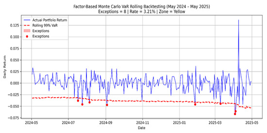
Figure 5.
Factor-based Monte Carlo VaR rolling backtesting.
Figure 4 shows the rolling backtesting results of the return-based Monte Carlo model. For each day in the 249-day testing window from May 2024 to May 2025, the VaR estimate is recalculated using a 250-day lookback window. This dynamic estimation approach captures evolving market behavior without assuming static risk parameters. The exceptions are flagged where the daily portfolio returns fall below the rolling 99% VaR threshold.
Figure 5 presents the rolling backtesting performance of the factor-based Monte Carlo model, applying the same 250-day rolling window methodology. While both of the models benefit from the dynamic recalibration, the factor-based model exhibits a lower exception count (8 vs. 11), resulting in an improved regulatory classification (yellow vs. red). This reflects the differences in the tail risk behavior due to the incorporation of systematic exposures.
These results reveal how rolling recalibration affects the model responsiveness and exception clustering. A more detailed comparison between the standard and rolling backtesting outcomes is presented in Section 4.3.
4.3. Discussion of Backtesting Results
This Section compares the results of the standard and rolling backtesting frameworks to assess how the model recalibration frequency affects the exception behavior and regulatory classification. While both of the approaches rely on the same underlying portfolio and simulation models, the resulting exception counts reveal meaningful differences in performance.
Under the standard backtest, both the return-based and factor-based Monte Carlo models produce 13 exceptions, placing them in the Basel red zone. When switching to a rolling-window framework, the exception counts decrease for both of the models, reflecting an improved responsiveness to evolving market conditions. Specifically, the return-based model yields 11 exceptions under the rolling backtesting, which remains in the red zone but shows a slight reduction in the exception count compared to the standard backtest, while the factor-based model reduces its exception count to 8, improving its regulatory classification to the yellow zone. This shift highlights the benefit of dynamically updating the risk estimates based on evolving market conditions.
From a regulatory perspective, rolling backtesting enhances the timeliness and sensitivity of the risk measurement. By estimating VaR using recent data, the model becomes more adaptive to current volatility conditions and more responsive to abrupt shifts in market risk. This approach aligns with the expectations outlined in FDIC FIL-26-2012, which emphasizes robust model performance monitoring and the importance of accurate capital determination for trading book exposures (Federal Deposit Insurance Corporation 2012).
In addition to the exception counts, we further evaluate model performance using Christoffersen’s (1998) conditional coverage framework. The main results are discussed below, while additional statistical outputs and implementation details are provided in Table A2 in Appendix C, along with further implementation details. The results show that both of the rolling VaR models pass the conditional independence test but fail the unconditional coverage test, indicating that while the violations do not exhibit significant clustering, their overall frequency exceeds the expected level under a 99% confidence threshold. These findings suggest that the current models may underestimate extreme tail risk. All the data and implementation code used in this study are publicly available via GitHub (see Appendix D for details). As a future extension, we propose incorporating GARCH-based volatility modeling to address the limitations of constant-variance assumptions and improve the tracking of volatility clustering.
5. Conclusions
This study compares return-based and factor-based Monte Carlo VaR models under both standard and rolling backtesting frameworks. While both of the approaches produce similar VaR estimates in non-stressed market environments, their performance diverges when the market conditions become volatile. Rolling recalibration improves the model responsiveness, particularly for the factor-based model, which captures risk factor co-movements and structural breaks more effectively under volatile conditions.
The return-based model is appealing for its simplicity and ease of implementation. Although both of the models are inherently backward-looking, their ability to adjust to sudden volatility changes differs. The return-based model may underreact more acutely due to its simplified structure and dependence on historical return distributions. In contrast, the factor-based model captures cross-asset co-movements and demonstrates improved resilience in volatile regimes, particularly when paired with the rolling VaR estimation. These differences highlight the trade-off between simplicity and structural sensitivity in VaR modeling, which should be carefully balanced when aligning with regulatory objectives under Basel III.
One promising extension is to adapt the factor-based simulation framework for stress testing by replacing the rolling estimation window with historical crisis periods, such as the 2008 financial crisis. This approach recalibrates the factor return distribution to stress-period dynamics, enabling the VaR estimation to reflect adverse market regimes in line with scenario-based capital planning. Alternatively, factor shocks can be injected into the simulation paths to replicate forward-looking supervisory scenarios, consistent with the practices seen in the CCAR and the Basel III stress testing (Federal Reserve Board 2023).
These findings reinforce the value of rolling backtesting and simulation flexibility in achieving Basel III compliance. Institutions aiming for internal model approval may benefit from combining the rolling VaR estimation with structurally aware simulation frameworks such as the factor-based approach.
Funding
This research received no external funding.
Data Availability Statement
The simulation code and visualization notebooks are available at: https://github.com/Chengyueminga/MarketRisk_VaR (accessed on 10 June 2025). The input data were retrieved directly from public financial sources, specifically Yahoo Finance, and are not included in the repository. However, the provided code contains clear instructions for replicating the data download process, ensuring full reproducibility.
Conflicts of Interest
The author declares no conflict of interest.
Disclaimer
Views expressed are that of the author and do not necessarily represent the views of the author’s employer.
Appendix A

Figure A1.
Flowchart of the Monte Carlo VaR modeling and Basel III backtesting framework.
Both return-based and factor-based models follow a shared pipeline comprising data input, parameter calibration, Monte Carlo simulation, VaR estimation, and exception backtesting. The process is designed to be modular and fully reproducible using public data. Model outputs are evaluated under the Basel Committee’s traffic light framework to determine regulatory classification and model adequacy.
Appendix B
The sample quantiles align closely with the theoretical quantiles from a standard normal distribution, indicating that the OLS residuals are approximately normally distributed. This validates the use of p-values for factor selection.
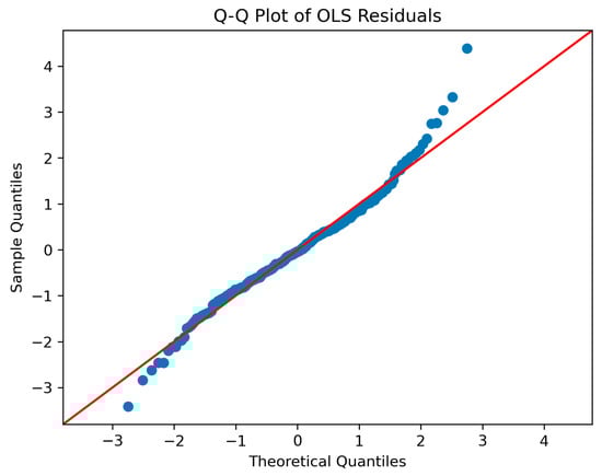
Figure A2.
Q–Q plot of OLS residuals.
Each line represents the estimated coefficient of a factor across a sequence of regularization parameters (lambda) in log scale. Dominant variables (e.g., XLK, IWF) emerge early and maintain strong coefficients, while redundant or weak predictors (e.g., TLT, ^VIX) are shrunk toward zero.

Figure A3.
LASSO coefficient path for factor selection.
Table A1 reports the bootstrapped 95% confidence intervals for the VaR estimates shown in Table 2, reflecting the uncertainty from Monte Carlo simulation.
Table A1.
95% Confidence intervals for simulated 99% one-day VaR estimates.
Table A1.
95% Confidence intervals for simulated 99% one-day VaR estimates.
| Method | VaR (99%) | 95% CI |
|---|---|---|
| Return-Based MC | 3.26% | [3.23%, 3.44%] |
| Factor-Based MC | 3.10% | [3.04%, 3.17%] |
Appendix C. Christoffersen’s Conditional Coverage Framework Test Result
To supplement the exceedance-based backtesting in Section 4, we apply Christoffersen’s conditional coverage framework to assess whether the sequence of VaR violations is statistically consistent with the expected behavior under the model. This test combines two components:
- Unconditional Coverage (UC): evaluates whether the total number of exceptions matches the expected frequency.
- Conditional Coverage (CC): further tests whether exceptions are independently distributed over time, detecting potential clustering that may indicate model misspecification.
For both rolling backtesting models, the conditional independence component is satisfied, but the Unconditional Coverage test is rejected at the 5% significance level. These results are summarized in Table A2, and they suggest that while violations are not significantly clustered, the models tend to underestimate extreme risk.
Table A2.
Christoffersen test results for rolling VaR models.
Table A2.
Christoffersen test results for rolling VaR models.
| Model | UC p-Value | CC p-Value | Result |
|---|---|---|---|
| Return-Based MC | 0.00 | 0.50 | CC pass, UC fail |
| Factor-Based MC | 0.01 | 0.24 | CC pass, UC fail |
Appendix D. Code and Data Availability
The full simulation code, input data, and visualization notebooks used in this study are publicly available at the following GitHub repository: https://github.com/Chengyueminga/MarketRisk_VaR (accessed on 10 June 2025)
The table below summarizes the key files and their functions.
| File | Description |
| Basel3-VaR-Backtest_Monte-Carlo-Simulation.ipynb | Monte Carlo VaR simulation using historical return sampling. |
| Beta-Based Risk Factor VaR Simulation for Basel III Backtesting.ipynb | Factor-driven VaR simulation based on CAPM-style regression. |
| VaR_Comparison.ipynb | Consolidated visualization and backtesting comparison of both models. |
| README.md | Documentation on structure, assumptions, and usage. |
| License | MIT License. |
| Last Updated | May 2025. |
This repository is designed to enable full reproducibility. Readers are encouraged to clone or download the codebase and replicate the experiments for educational or benchmarking purposes.
References
- Alexander, Carol. 2009. Market Risk Analysis, Volume IV: Value-at-Risk Models. Chichester: John Wiley & Sons. [Google Scholar]
- Barkhagen, Mathias, Sergio García, Jacek Gondzio, Jörg Kalcsics, J. Kroeske, Sotirios Sabanis, and A. Staal. 2023. Optimising Portfolio Diversification and Dimensionality. Journal of Global Optimization 85: 185–234. [Google Scholar] [CrossRef]
- Basel Committee on Banking Supervision. 1996. Supervisory Framework for the Use of Backtesting in Conjunction with the Internal Models Approach to Market Risk Capital Requirements. Basel: Bank for International Settlements. [Google Scholar]
- Basel Committee on Banking Supervision. 2011. Principles for Sound Liquidity Risk Management and Supervision. Basel: Bank for International Settlements. [Google Scholar]
- Basel Committee on Banking Supervision. 2019. Minimum Capital Requirements for Market Risk. Basel: Bank for International Settlements. [Google Scholar]
- Board of Governors of the Federal Reserve System and Office of the Comptroller of the Currency. 2011. Supervisory Guidance on Model Risk Management (SR 11-7/OCC 2011-12); Washington, DC: Federal Reserve and OCC. Available online: https://www.occ.treas.gov/news-issuances/bulletins/2011/bulletin-2011-12a.pdf (accessed on 10 June 2025).
- Bodie, Zvi, Alex Kane, and Alan J. Marcus. 2014. Investments, 10th ed. New York: McGraw-Hill Education. [Google Scholar]
- Chatterjee, Samprit, and Ali S. Hadi. 2015. Regression Analysis by Example, 5th ed. Hoboken: John Wiley & Sons. [Google Scholar]
- Christoffersen, Peter F. 1998. Evaluating Interval Forecasts. International Economic Review 39: 841–62. [Google Scholar] [CrossRef]
- Embrechts, Paul, Alexander McNeil, and Daniel Straumann. 2002. Correlation and Dependence in Risk Management: Properties and Pitfalls. In Risk Management: Value at Risk and Beyond. Edited by M. A. H. Dempster. Cambridge: Cambridge University Press, pp. 176–223. [Google Scholar]
- Embrechts, Paul, Giovanni Puccetti, Ludger Rüschendorf, Ruodu Wang, and Antonela Beleraj. 2014. An Academic Response to Basel 3.5. Risks 2: 25–48. [Google Scholar] [CrossRef]
- Fama, Eugene F., and Kenneth R. French. 2015. A Five-Factor Asset Pricing Model. Journal of Financial Economics 116: 1–22. [Google Scholar] [CrossRef]
- Federal Deposit Insurance Corporation. 2012. FIL-26-2012: Risk-Based Capital Rules—Market Risk Final Rule; Washington, DC: FDIC, Note: Archived/Inactive. Available online: https://www.fdic.gov/news/inactive-financial-institution-letters/2012/fil12026.html (accessed on 10 June 2025).
- Federal Reserve Board. 2023. Supervisory Stress Test Methodology—June 2023; Washington, DC: Board of Governors of the Federal Reserve System. Available online: https://www.federalreserve.gov/publications/files/2023-june-supervisory-stress-test-methodology.pdf (accessed on 10 June 2025).
- Glasserman, Paul. 2004. Monte Carlo Methods in Financial Engineering. New York: Springer. [Google Scholar]
- Hull, John C. 2015. Risk Management and Financial Institutions, 4th ed. Hoboken: Wiley. [Google Scholar]
- Hull, John C. 2021. Options, Futures, and Other Derivatives, 11th ed. Harlow: Pearson. [Google Scholar]
- James, Gareth, Daniela Witten, Trevor Hastie, and Robert Tibshirani. 2013. An Introduction to Statistical Learning: With Applications in R. New York: Springer. [Google Scholar]
- Jorion, Philippe. 2007. Value at Risk: The New Benchmark for Managing Financial Risk, 3rd ed. New York: McGraw-Hill. [Google Scholar]
- Kutner, Michael H., Christopher J. Nachtsheim, John Neter, and William Li. 2005. Applied Linear Statistical Models, 5th ed. New York: McGraw-Hill Irwin. [Google Scholar]
- McNeil, Alexander J., Rüdiger Frey, and Paul Embrechts. 2015. Quantitative Risk Management: Concepts, Techniques and Tools. revised ed. Princeton: Princeton University Press. [Google Scholar]
- Menard, Scott. 2001. Applied Logistic Regression Analysis, 2nd ed. Thousand Oaks: Sage Publications. [Google Scholar]
- Meucci, Attilio. 2009. Risk and Asset Allocation. Berlin: Springer. [Google Scholar]
- Morningstar. 2021. Portfolio Snapshot Report Guide. Morningstar Direct. Available online: https://advisor.morningstar.com/enterprise/VTC/PortfolioSnapshotReport.pdf (accessed on 18 July 2025).
- MSCI. 2021. Barra Global Equity Model Handbook. MSCI Inc.: Available online: https://www.alacra.com/alacra/help/barra_handbook_gem.pdf (accessed on 18 July 2025).
- O’Brien, Robert M. 2007. A Caution Regarding Rules of Thumb for Variance Inflation Factors. Quality & Quantity 41: 673–90. [Google Scholar] [CrossRef]
- Pritsker, Matthew. 1997. Evaluating Value at Risk Methodologies: Accuracy versus Computational Time. Journal of Financial Services Research 12: 201–42. [Google Scholar] [CrossRef]
Disclaimer/Publisher’s Note: The statements, opinions and data contained in all publications are solely those of the individual author(s) and contributor(s) and not of MDPI and/or the editor(s). MDPI and/or the editor(s) disclaim responsibility for any injury to people or property resulting from any ideas, methods, instructions or products referred to in the content. |
© 2025 by the author. Licensee MDPI, Basel, Switzerland. This article is an open access article distributed under the terms and conditions of the Creative Commons Attribution (CC BY) license (https://creativecommons.org/licenses/by/4.0/).