Evaluation of Perpetual American Put Options with General Payoff

Abstract

In this paper, we study perpetual American put options with a generalized standard put payoff and establish sufficient conditions for the existence and uniqueness of the solution to the associated pricing problem. As a key tool, we express the Black–Scholes operator in terms of elasticity. This formulation enables us to demonstrate that the considered pricing problem admits a unique solution when the payoff function exhibits strictly decreasing elasticity with respect to the underlying asset. Furthermore, this approach allows us to derive closed-form solutions for option pricing.

1. Introduction

Financial derivatives are important hedging instruments that allow for the management of risks associated with high volatility and uncertainty, as they derive their current value from an underlying commodity or asset (Islam and Chakraborti 2015). An option is a financial contract allowing the holder to buy (call option) or sell (put option) an underlying asset, such as a stock, at a predetermined strike price before a specified expiration date. European options can only be exercised at expiration, while American options can be exercised anytime up to the expiration date. Perpetual options, unlike standard options, can be exercised at any time indefinitely, as they never expire (Gapeev and Al Motairi 2018). The literature contains numerous studies on perpetual American options (Rodrigo 2022).

In recent years, options with piecewise linear payoff functions have attracted increasing research interest across a broad spectrum of contexts (Lee et al. 2021). Numerous studies have also explored non-linear payoff functions, such as power options (Esser 2003; Fadugba and Nwozo 2020; Heynen and Kat 1996; Rodrigo 2022; Tompkins 2000; Zhang 1997) and polynomial options (Macovschi and Quittard-Pinon 2006). Power options, also known as leveraged options, are distinguished by their non-linear payoff structure, which depends on the underlying asset raised to a given power. This feature provides investors with the potential for substantially higher returns compared to standard vanilla options Ha et al. (2025). Further references on option pricing with non-linear payoffs can be found in Ibrahim et al. (2012); Lee (2020); Lee et al. (2020); Liu and Lio (2024); Nualsri and Mekchay (2022). See also Feng and Quan (2010) for power options and Wang et al. (2022) for polynomial options.

Following this research direction, in this study we deal with the problem of pricing perpetual American put options with a generalized standard put payoff $Y_t=G\left(S_t\right)$, where $S_t$ is the underlying asset price at time t, and $G=G\left(S\right)$ is the payoff function. The payoff function G is assumed to be a continuously decreasing function such that $G\left(S\right)>0$ for all $0\le S<K$, and $G\left(S\right)=0$ for all $S\ge K$, where K is the contracted strike price.

It is well known (see Karatzas 1988; Karatzas and Shreve 1998; MacKean 1965; Merton 1973; Samuelson 1965) that the price of a perpetual American put option with the standard payoff function $G\left(S\right)=max\{K-S,0\}$ can be found by solving an associated free-boundary problem. In this formulation, using the Black–Scholes model, we seek a critical price $S_c\in ]0,K[$ and a pricing function $V=V\left(S\right)$ such that $V=G$ in the exercise region $\{S:S\le S_c\}$, and, in the case of no dividends, the linear ordinary differential equation

$${\displaystyle \frac{1}{2}}{\sigma }^2{S}^2{\displaystyle \frac{d^{2}V}{d{S}^2}}+rS{\displaystyle \frac{dV}{dS}}-rV=0$$

holds in the continuation region $\{S:S>S_c\}$. The critical price $S_c$ separates the exercise region, where it is optimal to exercise the option, from the continuation region, where it is best to hold the option. Note that $S_c$ is not known a priori and is thus referred to as a free boundary, determined using the value-matching and smooth-pasting conditions $V\left(S_c\right)=G\left(S_c\right)$ and ${\displaystyle \frac{dV}{dS}}\left(S_c\right)={\displaystyle \frac{dG}{dS}}\left(S_c\right)$, which are required to avoid arbitrage opportunities. These conditions ensure that the price and its first derivative are both continuous. Moreover, the inequality

$${\displaystyle \frac{1}{2}}{\sigma }^2{S}^2{\displaystyle \frac{d^{2}G}{d{S}^2}}+rS{\displaystyle \frac{dG}{dS}}-rG<0$$

must hold in the exercise region $S<S_c$, to ensure the construction of a strategy that super-replicates the option payoff (for details, see the proof of Theorem A1 in Appendix A, Equation (A10)). We observe that for the standard payoff function $G\left(S\right)=max\{K-S,0\}$, the previous inequality holds because in the exercise region, it gives $G\left(S\right)=K-S$, and thus,

$${\displaystyle \frac{1}{2}}{\sigma }^2{S}^2{\displaystyle \frac{d^{2}V}{d{S}^2}}+rS{\displaystyle \frac{dV}{dS}}-rV=-rK<0,$$

since $r,K>0$. However, for an option with a general non-concave payoff function, the above inequality is not guaranteed to be satisfied.

In this paper, we establish sufficient conditions on the payoff function to ensure both that the above inequality holds within the exercise region and that the free-boundary problem associated with the pricing of a perpetual American put option admits a unique solution. To achieve this, we provide a novel expression for the Black–Scholes operator in terms of elasticity (see Proposition 1). To the best of our knowledge, this result has not yet appeared in the literature. Using this new formulation, we will show that for payoff functions with strictly decreasing elasticity, the associated free-boundary problem admits a unique solution. This also enables the derivation of closed-form solutions for the option price.

A notable contribution in this area is the work by Rodrigo (2022), who derives pricing formulas for perpetual American options with general payoffs, primarily focusing on piecewise linear functions. In that contribution, the analysis is oriented toward the structural properties and support of the payoff function and includes various types of options, such as calls and straddles. In contrast, the present study focuses on perpetual American put options with a class of generalized standard put payoffs, which includes non-linear forms such as power and polynomial options—extending beyond the piecewise linear framework considered in Rodrigo’s work. Moreover, our approach is inspired by the methodology introduced in Karatzas and Shreve (1998), where the pricing problem for standard payoffs is shown to be equivalent to a free-boundary problem. We adopt this perspective and develop a novel analytical framework based on the concept of elasticity, a key economic indicator that captures the responsiveness of the payoff to changes in the underlying asset. By expressing the Black–Scholes operator in terms of elasticity, we derive sufficient conditions under which the associated free-boundary problem admits a unique solution.

The remainder of the paper is organized as follows. The mathematical formulation of the pricing problem is developed and the main results are given in Section 2. In Section 3, we apply our findings to some classes of perpetual American put options with non-linear payoffs. Conclusions are drawn in Section 5. Additionally, in Appendix A we show that the formulation of the pricing problem as a free-boundary problem is still valid in the case of generalized standard put payoffs.

2. Pricing of Perpetual American Put Options with Generalized Standard Put Payoff

In this section we formulate the free-boundary problem associated with option pricing and state our main results.

We consider a perpetual American put option with payoff at time t given by $Y_t=G\left(S_t\right)$. The payoff function $G=G\left(S\right)$ is assumed to be a non-negative decreasing continuous function on $[0,+\infty [$ such that $G\left(S\right)>0$ for all $0\le S<K$, and $G\left(S\right)=0$ for all $S\ge K$, with $K>0$. We also assume that $G\in C^2\left(\right]0,K\left[\right)$. Note in particular that these assumptions are satisfied by the standard payoff $G\left(S\right)=max\{K-S,0\}$ of a vanilla put option, where K is the contracted strike price. We assume that the underlying asset price process $S_t$ satisfies the standard Black–Scholes model

$$d{S}_t=\left(r-\delta \right)S_{t}dt+\sigma S_{t}d{Z}_t,S_0>0,$$

(1)

where r is the risk-free interest rate, $\delta$ is the dividend yield, $\sigma$ is the volatility of the stock, and $Z_t$ is a Wiener process with respect to the risk-neutral probability measure. Here, the parameters $r>0$, $\delta \ge 0$, and $\sigma >0$ are assumed to be constants.

By extending the approach proposed in Karatzas (1988); Karatzas and Wang (2000); Karatzas and Shreve (1998); Peskir and Shiryaev (2006) for the case of standard payoff, in the following we formulate the pricing problem of a perpetual American put option with a generalized standard put payoff as a free-boundary problem. In Appendix A (see Theorem A1), we show the validity of this formulation.

The free-boundary problem associated with a perpetual American put option with payoff function $G=G\left(S\right)$ can be expressed as follows.

Problem 1.

Find a free boundary $S_c\in ]0,K[$ and a decreasing function $V=V\left(S\right)$ in the space $C^0\left([0,+\infty [\right)\cap C^1\left(]0,+\infty [\right)\cap C^2\left(]0,+\infty [\setminus \left\{S_c\right\}\right)$ such that

$$\begin{array}{cc}\hfill {\displaystyle \frac{1}{2}}{\sigma }^2{S}^2{\displaystyle \frac{d^{2}V}{d{S}^2}}+(r-\delta )S{\displaystyle \frac{dV}{dS}}-rV=0& S_c<S<+\infty \hfill \end{array}$$

(2)

$$\begin{array}{cc}\hfill {\displaystyle \frac{1}{2}}{\sigma }^2{S}^2{\displaystyle \frac{d^{2}V}{d{S}^2}}+(r-\delta )S{\displaystyle \frac{dV}{dS}}-rV<0& 0<S<S_c\hfill \end{array}$$

(3)

$$\begin{array}{cc}\hfill V\left(S\right)>G\left(S\right)& S_c<S<+\infty \hfill \end{array}$$

(4)

$$\begin{array}{cc}\hfill V\left(S\right)=G\left(S\right)& 0\le S\le S_c\hfill \end{array}$$

(5)

$$\begin{array}{cc}\hfill 0\le -S{\displaystyle \frac{dV}{dS}}\le c& 0<S<+\infty \hfill \end{array}$$

(6)

for some constant $c>0$.

The solution V is usually referred to as the value function or option pricing function, and the free boundary $S_c$ is known as the optimal exercise price or critical stock price. Moreover, by considering the Black–Scholes operator given by

$$\mathcal{L}V={\displaystyle \frac{1}{2}}{\sigma }^2{S}^2{\displaystyle \frac{d^{2}V}{d{S}^2}}+(r-\delta )S{\displaystyle \frac{dV}{dS}}-rV,$$

in the exercise region $\{S:S<S_c\}$, it is optimal to exercise the option, since $\mathcal{L}V<0$, and therefore, the option value is $V\left(S\right)=G\left(S\right)$. In the continuation region $\{S:S>S_c\}$ it is not optimal to exercise the option, and thus, the option value satisfies $\mathcal{L}V=0$.

By inspecting the proof of Theorem A1 (see Appendix A), we observe that the condition (3) of Problem 1, specifically $\mathcal{L}G<0$ for $S<S_c$, enables us to achieve (A10) and thus allows us to construct a strategy that super-replicates the payoff of the option. As we have shown in Remark 1, in the case of standard payoff, this condition can be directly derived by computation.

Remark 1.

For a perpetual American put option with standard payoff $G\left(S\right)=max\left\{K-S,0\right\}$, the solution $(S_c,V)$ to Problem 1 is given by (see Karatzas and Shreve 1998)

$$S_c={\displaystyle \frac{{\beta }_{1}K}{{\beta }_1-1}}$$

and

$$V\left(S\right)=\left\{\begin{array}{cc}K-S\hfill & 0\le S\le S_c\hfill \\ (K-S_c){\left({\displaystyle \frac{S_c}{S}}\right)}^{-{\beta }_1}\hfill & S_c<S<+\infty ,\hfill \end{array}\right.$$

where ${\beta }_1$ is the negative solution to (13) given by (14).

The proof of this result proceeds using analogous arguments to those in the initial part of the demonstration of Theorem 1, which will be presented subsequently. Specifically, we emphasize that, in this case, condition (3) can be established by demonstrating that

$${\displaystyle \frac{1}{2}}{\sigma }^2{S}^2{\displaystyle \frac{d^{2}G}{d{S}^2}}+(r-\delta )S{\displaystyle \frac{dG}{dS}}-rG=\delta S-rK<0,0<S<S_c.$$

(7)

The equality

$${\displaystyle \frac{1}{2}}{\sigma }^2{S}^2{\displaystyle \frac{d^{2}G}{d{S}^2}}+(r-\delta )S{\displaystyle \frac{dG}{dS}}-rG=\delta S-rK,0<S<S_c,$$

is derived directly by computation, noting that for $S<S_c$ we have $G\left(S\right)=K-S$. Furthermore, for $S<S_c={\beta }_{1}K/({\beta }_1-1)$, the inequality

$$\delta S-rK<\delta S_c-rK=\delta {\displaystyle \frac{{\beta }_{1}K}{{\beta }_1-1}}-rK=-{\displaystyle \frac{(r-\delta ){\beta }_1-r}{{\beta }_1-1}}K<0$$

holds because ${\beta }_1<0$ and $(r-\delta ){\beta }_1<r$, since

$$(r-\delta ){\beta }_1-r<(r-\delta ){\beta }_1-r+{\displaystyle \frac{1}{2}}{\sigma }^2{\beta }_1^2-{\displaystyle \frac{1}{2}}{\sigma }^2{\beta }_1={\displaystyle \frac{1}{2}}{\sigma }^2{\beta }_1^2-\left({\displaystyle \frac{1}{2}}{\sigma }^2-r+\delta \right){\beta }_1-r=0,$$

where the last equality follows from the fact that ${\beta }_1$ is a solution to Equation (13).

Our aim is to provide sufficient conditions on a generalized standard put payoff function G of a perpetual American put option such that both the inequality (3) holds within the exercise region and Problem 1 admits a unique solution. We start with noting that if $(S_c,V)$ is a solution to Problem 1 the following boundary conditions, known as the value-matching and smooth-pasting conditions,

$$V\left(S_c\right)=G\left(S_c\right),{\displaystyle \frac{dV}{dS}}\left(S_c\right)={\displaystyle \frac{dG}{dS}}\left(S_c\right)$$

(8)

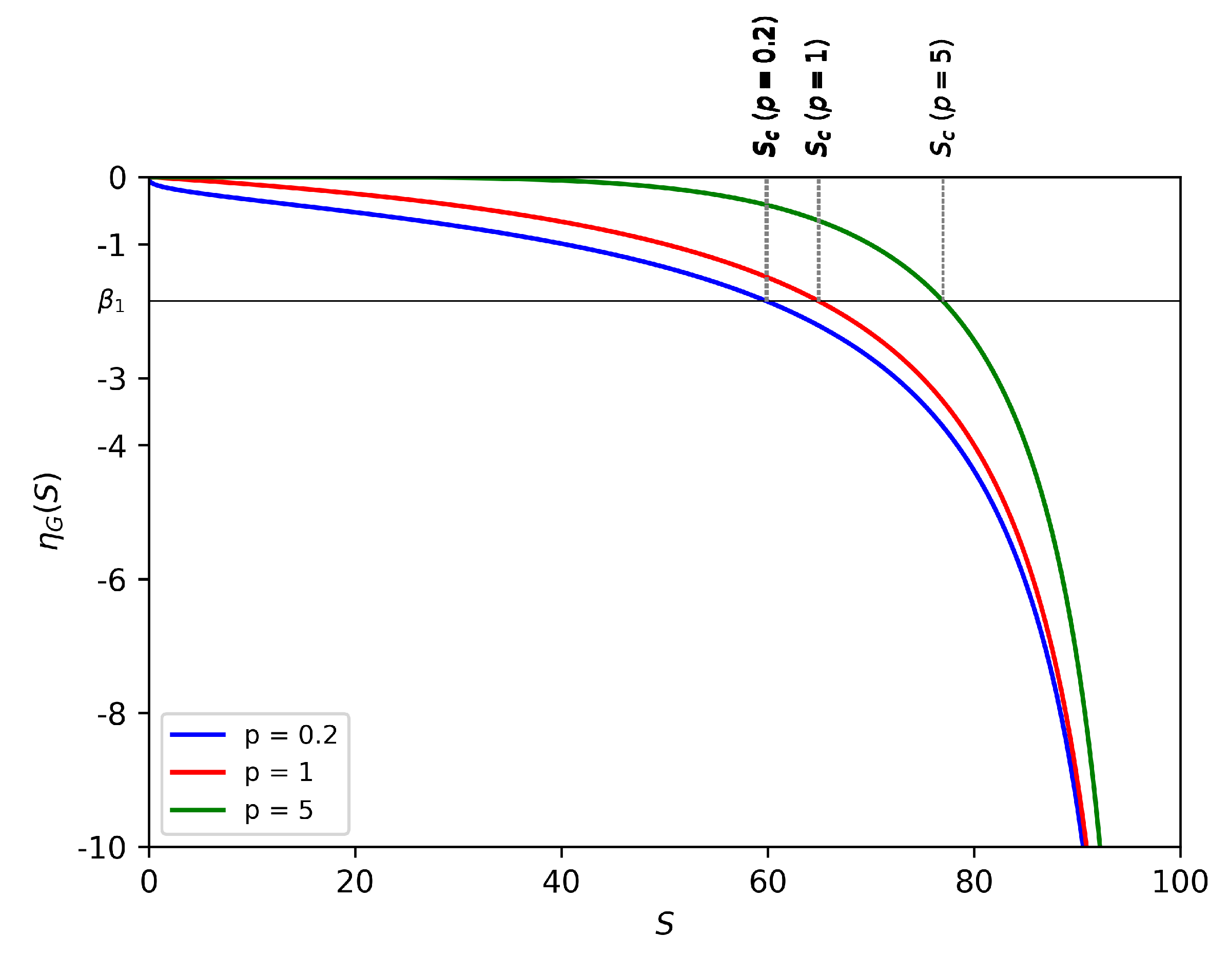
must be satisfied to ensure the continuity of both the price and its first derivative. We first observe that, due to the boundary conditions (8), it is evident that at critical price $S_c$, the elasticity of the payoff function aligns with the elasticity of the option value function, namely

$${\eta }_V\left(S_c\right)={\eta }_G\left(S_c\right),$$

(9)

where the elasticity function ${\eta }_G={\eta }_G\left(S\right)$ of G is defined for $S\in ]0,K[$ by (note that $G\left(S\right)>0$ for $0\le S<K$)

$${\eta }_G\left(S\right)={\displaystyle \frac{S}{G\left(S\right)}}{\displaystyle \frac{dG}{dS}}\left(S\right),$$

(10)

and the elasticity ${\eta }_V={\eta }_V\left(S\right)$ of V is

$${\eta }_V\left(S\right)={\displaystyle \frac{S}{V\left(S\right)}}{\displaystyle \frac{dV}{dS}}\left(S\right).$$

Note that, in the case of put options, the elasticity is negative.

Inspired by (9), we focused on the elasticity of the payoff function G to identify sufficient conditions to ensure that Problem 1 admits a solution. To this end, in the next Proposition we provide a novel expression for the Black–Scholes operator in terms of the elasticity of the payoff.

Proposition 1.

Let D be an open subset of the real line $\mathbb{R}$, and $F=F\left(S\right)$ a function $C^2\left(D\right)$, such that $F\left(S\right)>0$ for all $S\in D$. Then the operator defined by

$$\mathcal{L}F={\displaystyle \frac{1}{2}}{\sigma }^2{S}^2{\displaystyle \frac{d^{2}F}{d{S}^2}}+(r-\delta )S{\displaystyle \frac{dF}{dS}}-rF$$

(11)

can be expressed, for $S\in D$, as

$$\mathcal{L}F={\displaystyle \frac{1}{2}}{\sigma }^{2}FS{\displaystyle \frac{d{\eta }_F}{dS}}+{\displaystyle \frac{1}{2}}{\sigma }^{2}F\left({\eta }_F-{\beta }_1\right)\left({\eta }_F-{\beta }_2\right),$$

(12)

where ${\eta }_F={\eta }_F\left(S\right)$ is the elasticity function of F, and ${\beta }_1<0$ and ${\beta }_2>0$ are the solutions to the algebraic equation

$${\displaystyle \frac{1}{2}}{\sigma }^2{\beta }^2-\left({\displaystyle \frac{1}{2}}{\sigma }^2-r+\delta \right)\beta -r=0,$$

(13)

given by

$${\beta }_1={\displaystyle \frac{\left(\frac{1}{2}{\sigma }^2-r+\delta \right)-\sqrt{{\left(\frac{1}{2}{\sigma }^2-r+\delta \right)}^2+2{\sigma }^{2}r}}{{\sigma }^2}},$$

(14)

$${\beta }_2={\displaystyle \frac{\left(\frac{1}{2}{\sigma }^2-r+\delta \right)+\sqrt{{\left(\frac{1}{2}{\sigma }^2-r+\delta \right)}^2+2{\sigma }^{2}r}}{{\sigma }^2}}.$$

(15)

Proof. 

From the expression of elasticity ${\eta }_F={\displaystyle \frac{S}{F}}{\displaystyle \frac{dF}{dS}}$, it follows that

$${\displaystyle \frac{dF}{dS}}={\displaystyle \frac{F}{S}}{\eta }_F.$$

(16)

Furthermore, through computation, we obtain

$${\displaystyle \frac{d^{2}F}{d{S}^2}}={\displaystyle \frac{F}{S}}{\displaystyle \frac{d{\eta }_F}{dS}}+{\displaystyle \frac{F}{S^2}}{\eta }_F^2-{\displaystyle \frac{F}{S^2}}{\eta }_F.$$

(17)

Substituting (16) and (17) in (11), we obtain

$$\mathcal{L}F={\displaystyle \frac{1}{2}}{\sigma }^{2}FS{\displaystyle \frac{d{\eta }_F}{dS}}+{\displaystyle \frac{1}{2}}{\sigma }^{2}F{\eta }_F^2-\left({\displaystyle \frac{1}{2}}{\sigma }^2-r+\delta \right)F{\eta }_F-rF.$$

(18)

Since ${\beta }_1,{\beta }_2$ are the solutions to Equation (13), we can write

$${\displaystyle \frac{1}{2}}{\sigma }^2{\eta }_F^2-\left({\displaystyle \frac{1}{2}}{\sigma }^2-r+\delta \right){\eta }_F-r={\displaystyle \frac{1}{2}}{\sigma }^2\left({\eta }_F-{\beta }_1\right)\left({\eta }_F-{\beta }_2\right).$$

Using the last equality in (18), we obtain (12). □

Remark 2.

In the absence of dividends, that is, when $\delta =0$, we find from (14) and (15) that ${\beta }_1=-{\displaystyle \frac{2r}{{\sigma }^2}}$ and ${\beta }_2=1$. Therefore, from (12), we obtain the following expression:

$$\mathcal{L}F={\displaystyle \frac{1}{2}}{\sigma }^{2}FS{\displaystyle \frac{d{\eta }_F}{dS}}+{\displaystyle \frac{1}{2}}{\sigma }^{2}F\left({\eta }_F+{\displaystyle \frac{2r}{{\sigma }^2}}\right)\left({\eta }_F-1\right).$$

The result established in Proposition 1 provides a valuable expression for the Black–Scholes operator and enables the reformulation of condition (3) (i.e., $\mathcal{L}G\left(S\right)<0$ for $0<S<S_c$) in terms of the elasticity ${\eta }_G$. This formulation is useful for establishing the next theorem, our main result, which provides sufficient conditions for the existence of a unique solution to Problem 1.

For clarity and consistency of notation, we specify that, throughout this manuscript and in the Appendix, the symbols ${\beta }_1$ and ${\beta }_2$ refer exclusively to the solutions to Equation (13), defined in (14) and (15), respectively.

Theorem 1.

Consider a perpetual American put options with payoff $Y=G\left(S\right)$, where the payoff function $G=G\left(S\right)$ is a non-negative decreasing continuous function on $[0,+\infty [$ such that $G\left(S\right)>0$ for all $0\le S<K$, and $G\left(S\right)=0$ for all $S\ge K$, where $K>0$ is a suitable real constant. We also assume that $G\in C^2\left(\right]0,K\left[\right)$ and, furthermore, that the elasticity function ${\eta }_G={\eta }_G\left(S\right)$ of G is strictly decreasing. Then Problem 1 admits a unique solution $(S_c,V)$, where the boundary $S_c$ is the unique solution to the equation

$${\eta }_G\left(S_c\right)={\beta }_1$$

(19)

in the interval $]0,K[$, with ${\beta }_1<0$ given by (14), that is,

$${\beta }_1={\displaystyle \frac{\left(\frac{1}{2}{\sigma }^2-r+\delta \right)-\sqrt{{\left(\frac{1}{2}{\sigma }^2-r+\delta \right)}^2+2{\sigma }^{2}r}}{{\sigma }^2}},$$

and the value function $V=V\left(S\right)$ is

$$V\left(S\right)=\left\{\begin{array}{cc}G\left(S\right)\hfill & 0\le S\le S_c\hfill \\ G\left(S_c\right){\left({\displaystyle \frac{S_c}{S}}\right)}^{-{\beta }_1}\hfill & S_c<S<+\infty .\hfill \end{array}\right.$$

(20)

Proof. 

First, we observe that the linear ordinary differential equation $\mathcal{L}V=0$, i.e.,

$${\displaystyle \frac{1}{2}}{\sigma }^2{S}^2{\displaystyle \frac{d^{2}V}{d{S}^2}}+(r-\delta )S{\displaystyle \frac{dV}{dS}}-rV=0,$$

has solutions to the type $V\left(S\right)=B_1{S}^{{\beta }_1}+B_2{S}^{{\beta }_2}$, where ${\beta }_1<0$ and ${\beta }_2>0$ are the solutions to (13) given in (14) and (15), and $B_1,B_2\in \mathbb{R}$. Since we are looking for a decreasing function V, it follows that $B_2=0$, and so, $V\left(S\right)=B_1{S}^{{\beta }_1}$. Furthermore, the boundary condition $V\left(S_c\right)=G\left(S_c\right)$, with $S_c\in ]0,K[$, implies that $B_1=G\left(S_c\right)S_c^{-{\beta }_1}$. Therefore, the function

$$V\left(S\right)=\left\{\begin{array}{cc}G\left(S\right)\hfill & 0\le S\le S_c\hfill \\ G\left(S_c\right){\left({\displaystyle \frac{S_c}{S}}\right)}^{-{\beta }_1}\hfill & S_c<S<+\infty \hfill \end{array}\right.$$

(21)

is a decreasing function satisfying conditions (2) and (5). The value function V solution to Problem 1 is required to be $C^0\left([0,+\infty [\right)\cap C^1\left(]0,+\infty [\right)\cap C^2\left(]0,+\infty [\setminus \left\{S_c\right\}\right)$, and so, in order to ensure the regularity of V at boundary $S_c$, the smooth-pasting condition

$${\displaystyle \frac{dV}{dS}}\left(S_c\right)={\displaystyle \frac{dG}{dS}}\left(S_c\right)$$

must be satisfied. Since, from (21), we have $V\left(S\right)=G\left(S\right)$ for $0\le S\le S_c$, and ${\displaystyle \frac{dV}{dS}}\left(S\right)=G\left(S_c\right)S_c^{-{\beta }_1}{\beta }_1{S}^{{\beta }_1-1}$ for $S>S_c$, the condition ${\displaystyle \frac{dV}{dS}}\left(S_c\right)={\displaystyle \frac{dG}{dS}}\left(S_c\right)$ is verified if ${\displaystyle \frac{dG}{dS}}\left(S_c\right)=G\left(S_c\right)S_c^{-1}{\beta }_1$, that is, if ${\eta }_G\left(S_c\right)={\beta }_1$.

Thus we may conclude that Problem 1 admits a unique solution $(S_c,V)$ if the following conditions are satisfied:

(i)

There exists a unique solution $S_c$ to equation ${\eta }_G\left(S\right)={\beta }_1$ in the interval $]0,K[$;

(ii)

Properties (3), (4) and (6) hold.

We will show that the assumption of strictly decreasing elasticity payoff function is sufficient to ensure that (i) and (ii) are verified.

First, we will prove (i). For this, we consider the function f, defined as $f\left(S\right)=S^{-{\beta }_1}G\left(S\right)$. Observing that f is of class $C^0\left([0,K]\right)\cap C^1\left(]0,K[\right)$, and $f\left(0\right)=f\left(K\right)=0$, by applying Rolle’s Theorem it follows that there exists $S_c\in ]0,K[$ such that ${\displaystyle \frac{df}{dS}}\left(S_c\right)=0$. Through computation, we have

$${\displaystyle \frac{df}{dS}}\left(S\right)=G\left(S\right)S^{-{\beta }_1-1}\left({\eta }_G\left(S\right)-{\beta }_1\right),0<S<K$$

(22)

from which, since $G\left(S\right)>0$ for $S<K$, we deduce that ${\displaystyle \frac{df}{dS}}\left(S_c\right)=0$ implies that ${\eta }_G\left(S_c\right)-{\beta }_1=0$, and thus, ${\eta }_G\left(S_c\right)={\beta }_1$. The uniqueness of the solution $S_c$ follows from the assumption of the strict monotonicity of elasticity function ${\eta }_G$. So, we have proven (i).

We now prove (ii). Using (12) with $F=G$ and $D=]0,K[$, we have, for $S\in ]0,K[$,

$$\mathcal{L}G={\displaystyle \frac{1}{2}}{\sigma }^{2}GS{\displaystyle \frac{d{\eta }_G}{dS}}+{\displaystyle \frac{1}{2}}{\sigma }^{2}G\left({\eta }_G-{\beta }_1\right)\left({\eta }_G-{\beta }_2\right).$$

(23)

We observe that for all $S\in ]0,K[$, it follows that $G\left(S\right)>0$ and ${\displaystyle {\displaystyle \frac{d{\eta }_G}{dS}}\left(S\right)\le 0}$. Furthermore, if $S\in ]0,K[$ then ${\eta }_G\left(S\right)\le 0$, because ${\displaystyle {\eta }_G=\frac{S}{G}{\displaystyle \frac{dG}{dS}}}$, and G is decreasing, and thus, ${\eta }_G\left(S\right)-{\beta }_2<0$, since ${\beta }_2>0$. Moreover, from (i) we know that ${\eta }_G\left(S_c\right)-{\beta }_1=0$, and thus, by using the strictly decreasing property of ${\eta }_G$, it gives ${\eta }_G\left(S\right)-{\beta }_1>0$ for all $S\in ]0,S_c[$. Thus, from (23) we get $\mathcal{L}G<0$ for all $S\in ]0,S_c[$, that is, the condition (3).

Let us prove inequality (4), that is, $V\left(S\right)>G\left(S\right)$ for all $S>S_c$. Since $G\left(S\right)=0$ for all $S\ge K$, we only have to prove that the inequality holds in $]S_c,K[$. Thus, from (20), we have to show that for all $S\in ]S_c,K[$,

$$G\left(S_c\right){\left({\displaystyle \frac{S_c}{S}}\right)}^{-{\beta }_1}\ge G\left(S\right).$$

To this end, we consider again the function $f\left(S\right)=S^{-{\beta }_1}G\left(S\right)$, $S\ge 0$. Since ${\eta }_G\left(S_c\right)={\beta }_1$, and ${\eta }_G$ is strictly decreasing, from (22) we obtain for $S\in ]S_c,K[$

$${\displaystyle \frac{df}{dS}}\left(S\right)=G\left(S\right)S^{-{\beta }_1-1}\left({\eta }_G\left(S\right)-{\beta }_1\right)<0$$

from which, observing that ${\displaystyle \frac{df}{dS}}\left(S_c\right)=0$, it follows that f is strictly decreasing in $[S_c,K[$. Therefore, for all $S\in ]S_c,K[$, we can write

$$S_c^{-{\beta }_1}G\left(S_c\right)=f\left(S_c\right)>f\left(S\right)=S^{-{\beta }_1}G\left(S\right)$$

and thus, from (20),

$$V\left(S\right)=G\left(S_c\right){\left({\displaystyle \frac{S_c}{S}}\right)}^{-{\beta }_1}>G\left(S\right),$$

that is, the condition (4).

We must now prove (6). For this, we will prove that for all $S>0$,

$$0\le -S{\displaystyle \frac{dV}{dS}}\left(S\right)\le V\left(0\right)-S_c{\displaystyle \frac{dV}{dS}}\left(S_c\right),$$

(24)

from which (6) follows by letting $c=V\left(0\right)-S_c{\displaystyle \frac{dV}{dS}}\left(S_c\right)$. First, we consider the case $0<S<S_c$. Since ${\eta }_G$ is strictly decreasing we have ${\eta }_G\left(S\right)>{\eta }_G\left(S_c\right)$, and thus,

$$-{\displaystyle \frac{S}{G\left(S\right)}}{\displaystyle \frac{dG}{dS}}\left(S\right)<-{\displaystyle \frac{S_c}{G\left(S_c\right)}}{\displaystyle \frac{dG}{dS}}\left(S_c\right)$$

from which, taking into account that G is decreasing and positive, we obtain

$$-S{\displaystyle \frac{dG}{dS}}\left(S\right)<-S_c{\displaystyle \frac{G\left(S\right)}{G\left(S_c\right)}}{\displaystyle \frac{dG}{dS}}\left(S_c\right)\le -S_c{\displaystyle \frac{dG}{dS}}\left(S_c\right)\le G\left(0\right)-S_c{\displaystyle \frac{dG}{dS}}\left(S_c\right).$$

Observing that $V\left(S\right)=G\left(S\right)$ for $0<S<S_c$, we get (24). We now consider the case $S\ge S_c$. Since the function V given in (20) is convex in $[S_c,+\infty [$, we can write

$$V\left(S_c\right)\ge V\left(S\right)+{\displaystyle \frac{dV}{dS}}\left(S\right)(S_c-S)=V\left(S\right)-S{\displaystyle \frac{dV}{dS}}\left(S\right)+S_c{\displaystyle \frac{dV}{dS}}\left(S\right)$$

from which, observing that V is decreasing and positive, it follows that

$$0\le -S{\displaystyle \frac{dV}{dS}}\left(S\right)\le V\left(S_c\right)-V\left(S\right)-S_c{\displaystyle \frac{dV}{dS}}\left(S_c\right)\le V\left(0\right)-S_c{\displaystyle \frac{dV}{dS}}\left(S_c\right)$$

and thus, (24). The proof is therefore completed. □

Remark 3.

We observe that if $(S_c,V)$ is the solution to Problem 1 given by (19) and (20), it follows that

$${\eta }_V\left(S\right)=\left\{\begin{array}{cc}{\eta }_G\left(S\right)\hfill & 0<S\le S_c\hfill \\ {\eta }_G\left(S_c\right)={\beta }_1\hfill & S_c\le S<+\infty .\hfill \end{array}\right.$$

(25)

Remark 4.

We note that the conditions established in Theorem 1 are sufficient to ensure the existence and uniqueness of the solution to the associated free-boundary problem, and its consistency with the pricing problem. The question of whether these conditions are also necessary remains open and will be explored in future research.

3. Applications

In this section, we discuss the previous results by considering various classes of perpetual American put options with non-linear payoffs. For the numerical analysis, we used the following parameter settings: $\sigma =0.20$, $r=0.05$, $\delta =0.02$, and $K=100$. We remark that the adopted set of parameters has been frequently used in the literature (see, e.g., Aingworth et al. 2006; Martzoukos et al. 2024; Medvedev and Scaillet 2010; Necula et al. 2019; Zhang and Zhang 2024) for illustrative purposes. In this study, they are employed only to highlight the implications and interpretability of the results presented in the previous sections.

3.1. Perpetual American Power Put Options

Power options are a type of exotic option where the payoff at maturity is related to a positive power of the underlying asset price (see Heynen and Kat 1996; Macovschi and Quittard-Pinon 2006; Rodrigo 2022). Consider a perpetual power option with payoff

$$Y_t=max\left\{K^p-S_t^p,0\right\},p>0.$$

(26)

Note that for $p=1$, (26) represents the standard put option payoff. The payoff function $G\left(S\right)=max\left\{K^p-S^p,0\right\}$ is a non-negative, decreasing, continuous function on $[0,+\infty [$. Specifically, $G\left(S\right)>0$ for all $0\le S<K$, and $G\left(S\right)=0$ for all $S\ge K$. Furthermore, G satisfies the hypothesis of Theorem 1, as it has strictly decreasing elasticity given by

$${\eta }_G\left(S\right)=-{\displaystyle \frac{p{S}^p}{K^p-S^p}},0<S<K.$$

(27)

Figure 1 shows the elasticity ${\eta }_G={\eta }_G\left(S\right)$ for different values of parameter p. The boundary $S_c$ is determined to be the unique solution to the equation ${\eta }_G\left(S_c\right)={\beta }_1$. In this case, we can easily deduce that $S_c=K{\left({\displaystyle \frac{{\beta }_1}{{\beta }_1-p}}\right)}^{1/p}$.

To enhance the interpretation of our findings, Figure 2 illustrates the main functions discussed in the previous section, with reference to the perpetual power put option for different values of the parameter p. Specifically, in Figure 2a–c we show the payoff function G and the option price V computed from Equation (20). The critical price $S_c$ is also indicated. In Figure 2d–f we illustrate the elasticity ${\eta }_G$ of the payoff G. As expected, the elasticity is a negative and decreasing function. As previously shown in Figure 1, $S_c$ is the unique solution to the equation ${\eta }_G\left(S_c\right)={\beta }_1$. In Figure 2g–i we depict the behavior of the Black–Scholes (BS) operator $\mathcal{L}G\left(S\right)$ as a function of S. Note that condition (3) of Problem 1 is satisfied, since $\mathcal{L}G\left(S\right)<0$ for $S<S_c$. As a further clarification, we compare Figure 2a, Figure 2d, and Figure 2g, which illustrate, respectively, the payoff and value functions, the payoff elasticity, and the Black–Scholes operator for the case $p=0.2$. In Figure 2a, we observe that the separation between the payoff and value functions occurs at the critical price $S=S_c$, indicated by a vertical dashed line for easy identification. This critical point is also visible in the elasticity plot (Figure 2d) and the Black–Scholes operator plot (Figure 2g). Notably, the elasticity is always negative and strictly decreasing, while the Black–Scholes operator is negative in the region of interest, i.e., for $S<S_c$. Similar observations hold for the other parameter cases.

3.2. Perpetual American Powered Put Options

Consider a perpetual powered option (see Kim 2014) with payoff

$$Y_t={\left(max\left\{K-S_t,0\right\}\right)}^p,p>0.$$

(28)

The elasticity of the payoff function $G\left(S\right)={\left(max\left\{K-S,0\right\}\right)}^p$ is a strictly decreasing function given by

$${\eta }_G\left(S\right)=-{\displaystyle \frac{pS}{K-S}},0<S<K.$$

(29)

Figure 3 shows the elasticity ${\eta }_G={\eta }_G\left(S\right)$ for different values of parameter p.

In analogy with Figure 2, Figure 4 illustrates the behavior of elasticity and the Black–Scholes operator for the perpetual powered put option. Interestingly, we observe that for $p=5$, the Black–Scholes operator is not always negative. Nevertheless, due to the strictly decreasing property of elasticity ${\eta }_G$, condition (3) of Problem 1 is still satisfied, since $\mathcal{L}G\left(S\right)<0$ for $S<S_c$. This outcome is guaranteed by the strictly decreasing nature of elasticity ${\eta }_G$, as proven in Theorem 1.

3.3. Perpetual American General Power Put Options

We consider a perpetual American option with the payoff function (see Heynen and Kat 1996)

$$G\left(S\right)=max\left\{\sum _{i=1}^n{a}_i({(2K-S)}^i-K^i),0\right\},a_i\ge 0,n\in \mathbb{N}.$$

Observe that G is a non-negative decreasing continuous function on $[0,+\infty [$, such that $G\left(S\right)>0$ for all $0\le S<K$, and $G\left(S\right)=0$ for all $S\ge K$.

In the following Proposition, we establish some of the well known properties of elasticity.

Proposition 2.

The following properties hold for all $\alpha \ne 0$:

(i) 

${\eta }_{F^{\alpha }}=\alpha {\eta }_F$;

(ii) 

${\eta }_{\alpha F}={\eta }_F$;

(iii) 

${\eta }_{F·G}={\eta }_F+{\eta }_G$.

Using the properties established in Proposition 2, we can easily obtain the following expression for the elasticity of G:

$${\eta }_G\left(S\right)=-{\displaystyle \frac{n(n+1)}{2}}{\displaystyle \frac{S}{2K-S}},0<S<K.$$

(30)

Therefore, we can deduce that G has a strictly decreasing elasticity, and thus satisfies the hypotheses of Theorem 1.

4. Toward an Extension of Our Methodology to Perpetual American Call Options: Some Preliminary Results

To illustrate the broader applicability of the methodology developed in the preceding sections, we briefly explore its potential extension to the case of perpetual American call options. While a comprehensive analysis of this setting lies beyond the scope of the present work, the discussion below outlines how the framework—based on the concept of strictly decreasing elasticity of the payoff function—can be adapted to this context. A more detailed investigation will be pursued in future research.

It is important to note that the case of call options differs significantly from the put option case previously analyzed. As established in Karatzas and Shreve (1998), for the standard payoff function $G\left(S\right)=max\{S-K,0\}$, when the underlying stock pays no dividends (i.e., $\delta =0$), the value of the perpetual American call option equals the current stock price, i.e., $V\left(S\right)=S$. In this scenario, the optimal exercise price $S_c$ becomes infinite. Conversely (see Karatzas and Shreve 1998), when the conditions

$$\delta >0,r>\delta ,$$

(31)

hold, the associate free-boundary problem admits the solution $(S_c,V)$ given by

$$S_c={\displaystyle \frac{{\beta }_{2}K}{{\beta }_2-1}},$$

where ${\beta }_2$ is the positive solution to equation (13), as defined in (15), and

$$V\left(S\right)=\left\{\begin{array}{cc}(S_c-K){\left({\displaystyle \frac{S}{S_c}}\right)}^{{\beta }_2},\hfill & 0<S<S_c,\hfill \\ S-K,\hfill & S\ge S_c.\hfill \end{array}\right.$$

Note that for the standard call payoff $G\left(S\right)=max\{S-K,0\}$, the elasticity ${\mathcal{E}}_G\left(S\right)={\displaystyle \frac{S}{S-K}}$ is strictly decreasing for $S>K$. Moreover, it results in $\mathcal{L}G\left(S\right)<0$ for $S>S_c$, since

$$\mathcal{L}G\left(S\right)={\displaystyle \frac{1}{2}}{\sigma }^2{S}^2{\displaystyle \frac{d^{2}G}{d{S}^2}}+(r-\delta )S{\displaystyle \frac{dG}{dS}}-rG=-(\delta S-rK)<0,\mathrm{for}S>S_c.$$

This inequality follows from the fact that, under the assumption $r>\delta$, and using the bound $1<{\beta }_2<{\displaystyle \frac{r}{r-\delta }}$ (see, e.g., Karatzas and Shreve 1998), we obtain

$$\delta S-rK>\delta S_c-rK=\delta {\displaystyle \frac{{\beta }_{2}K}{{\beta }_2-1}}-rK=-{\displaystyle \frac{(r-\delta ){\beta }_2-r}{{\beta }_2-1}}K>0.$$

Building on these considerations, and in analogy with Theorem 1, we now provide sufficient conditions on a generalized standard call payoff function to allow for the resolution to the associated free-boundary problem. Unlike the put option payoff, which is bounded, the call option payoff is unbounded. Therefore, we require an appropriate growth condition on the payoff function.

Theorem 2.

Consider a perpetual American call option with payoff $Y=G\left(S\right)$, where the payoff function $G=G\left(S\right)$ is a non-negative, continuous, and increasing function on $[0,+\infty [$ satisfying $G\left(S\right)=0$ for all $0\le S\le K$, and $G\left(S\right)>0$ for all $S>K$, where $K>0$ is a suitable real constant. Assume further that $G\in C^2\left(\right]K,+\infty \left[\right)$ and that its elasticity function ${\eta }_G={\eta }_G\left(S\right)$ for G is strictly decreasing. Moreover, suppose the growth condition

$$\underset{S\to +\infty }{lim}{\displaystyle \frac{G\left(S\right)}{S^{{\beta }_2}}}=0$$

is satisfied, where ${\beta }_2$ is the positive root of Equation (13), as defined in (15). Let $S_c$ be the unique solution to the equation

$${\eta }_G\left(S_c\right)={\beta }_2$$

(32)

and define the value function $V=V\left(S\right)$ as

$$V\left(S\right)=\left\{\begin{array}{cc}G\left(S_c\right){\left({\displaystyle \frac{S}{S_c}}\right)}^{{\beta }_2}\hfill & 0\le S\le S_c\hfill \\ G\left(S\right)\hfill & S\ge S_c.\hfill \end{array}\right.$$

(33)

Then the pair $(S_c,V)$ is the unique solution to the following free-boundary problem:

$$\begin{array}{cc}\hfill {\displaystyle \frac{1}{2}}{\sigma }^2{S}^2{\displaystyle \frac{d^{2}V}{d{S}^2}}+(r-\delta )S{\displaystyle \frac{dV}{dS}}-rV=0& 0<S<S_c\hfill \end{array}$$

(34)

$$\begin{array}{cc}\hfill {\displaystyle \frac{1}{2}}{\sigma }^2{S}^2{\displaystyle \frac{d^{2}V}{d{S}^2}}+(r-\delta )S{\displaystyle \frac{dV}{dS}}-rV<0& S>S_c\hfill \end{array}$$

(35)

$$\begin{array}{cc}\hfill V\left(S\right)>G\left(S\right)& 0<S<S_c\hfill \end{array}$$

(36)

$$\begin{array}{cc}\hfill V\left(S\right)=G\left(S\right)& S\ge S_c.\hfill \end{array}$$

(37)

Proof. 

The general solution to the differential equation $\mathcal{L}V=0$ is of the form $V\left(S\right)=B_1{S}^{{\beta }_1}+B_2{S}^{{\beta }_2}$, where ${\beta }_1<0<{\beta }_2$ are the roots of Equation (13). Since we seek an increasing solution, we set $B_1=0$, yielding $V\left(S\right)=B_2{S}^{{\beta }_2}$. Imposing the boundary condition $V\left(S_c\right)=G\left(S_c\right)$, we obtain $B_2=G\left(S_c\right)S_c^{-{\beta }_2}$ and thus the expression in (33). Therefore, the increasing function defined in (33) satisfies conditions (34) and (37). Since we have $V\left(S\right)=G\left(S\right)$ for $S\ge S_c$, and ${\displaystyle \frac{dV}{dS}}\left(S\right)=G\left(S_c\right)S_c^{-{\beta }_2}{\beta }_2{S}^{{\beta }_2-1}$ for $S<S_c$, the smooth-pasting condition ${\displaystyle \frac{dV}{dS}}\left(S_c\right)={\displaystyle \frac{dG}{dS}}\left(S_c\right)$ is verified if ${\displaystyle \frac{dG}{dS}}\left(S_c\right)=G\left(S_c\right)S_c^{-1}{\beta }_2$, that is, if ${\eta }_G\left(S_c\right)={\beta }_2$.

Following an argument analogous to that used in the proof of Theorem 1, we prove that $(S_c,V)$ is the unique solution to the free-boundary problem by showing the following: (i) there exists a unique solution $S_c$ to equation ${\eta }_G\left(S\right)={\beta }_2$ in the interval $]K,+\infty [$; (ii) properties (35) and (36) hold. For this, we consider the function f of class $C^0\left([K,+\infty [\right)\cap C^1\left(]K,+\infty [\right)$ defined by $f\left(S\right)=S^{-{\beta }_2}G\left(S\right)$. From the growth condition, we have $f\left(K\right)=f(+\infty )=0$, and thus, there exists $S_c\in ]K,+\infty [$ such that ${\displaystyle \frac{df}{dS}}\left(S_c\right)=0$. From this, since

$${\displaystyle \frac{df}{dS}}\left(S\right)=G\left(S\right)S^{-{\beta }_2-1}\left({\eta }_G\left(S\right)-{\beta }_2\right),S>K,$$

and $G\left(S\right)>0$ for $S>K$, we deduce that ${\eta }_G\left(S_c\right)={\beta }_2$. The uniqueness of the solution $S_c$ follows from the assumption that ${\eta }_G$ is strictly decreasing. So, we have proven (i). We now prove (ii). Using (12) with $F=G$ and $D=]K.+\infty [$, we have, for $S\in ]K,+\infty [$,

$$\mathcal{L}G={\displaystyle \frac{1}{2}}{\sigma }^{2}GS{\displaystyle \frac{d{\eta }_G}{dS}}+{\displaystyle \frac{1}{2}}{\sigma }^{2}G\left({\eta }_G-{\beta }_1\right)\left({\eta }_G-{\beta }_2\right).$$

(38)

We observe that for $S>K$, we have $G\left(S\right)>0$, ${\displaystyle \frac{d{\eta }_G}{dS}}\left(S\right)\le 0$, and ${\eta }_G\left(S\right)-{\beta }_1>0$, since ${\beta }_1<0$ and ${\eta }_G\left(S\right)={\displaystyle \frac{S}{G}}{\displaystyle \frac{dG}{dS}}\ge 0$, because G is increasing. Moreover, ${\eta }_G\left(S\right)-{\beta }_2<0$ for all $S\in ]S_c,+\infty [$, since ${\eta }_G\left(S_c\right)-{\beta }_2=0$, and ${\eta }_G$ is strictly decreasing. Thus, from (38), we get $\mathcal{L}G<0$ for all $S\in ]S_c.+\infty [$, that is, (35).

We now prove (36). Since $G\left(S\right)=0$ for all $S\le K$, we only have to prove that $V\left(S\right)>G\left(S\right)$ in $]K,S_c[$. We observe that function $f\left(S\right)=S^{-{\beta }_2}G\left(S\right)$ is strictly increasing in $]K,S_c]$, since ${\displaystyle \frac{df}{dS}}\left(S_c\right)=0$ and ${\displaystyle \frac{df}{dS}}\left(S\right)=G\left(S\right)S^{-{\beta }_2-1}\left({\eta }_G\left(S\right)-{\beta }_2\right)>0$, because ${\eta }_G\left(S_c\right)={\beta }_2$, and ${\eta }_G$ is strictly decreasing. Therefore, for all $S\in ]K,S_c[$, we can write $S_c^{-{\beta }_2}G\left(S_c\right)=f\left(S_c\right)>f\left(S\right)=S^{-{\beta }_2}G\left(S\right)$ and thus, from (33),

$$V\left(S\right)=G\left(S_c\right){\left({\displaystyle \frac{S}{S_c}}\right)}^{{\beta }_2}>G\left(S\right).$$

This completes the proof. □

5. Conclusions and Future Perspectives

In this paper, we considered the problem of pricing perpetual American put options, allowing for a broader class of generalized standard put payoff functions. By establishing sufficient conditions on the payoff function, we ensured that the associated free-boundary problem admits a unique solution. To achieve this, we derived a novel expression for the Black–Scholes operator in terms of elasticity. Our main result demonstrates that for payoff functions with strictly decreasing elasticity, the pricing problem admits a unique solution.

Our findings extend the existing literature by investigating the relationship between payoff elasticity and the value of financial options. Additionally, the proposed approach enables the derivation of closed-form solutions for option prices in the case of non-linear payoffs, such as power options and powered options.

Future research could explore the application of this methodology to the hedging of the considered derivatives using elasticity, which measures the percentage change in the option price for a given percentage change in the asset price. Elasticity is always negative for put options, as noted by Sick and Gamba (2010), and its absolute value can be less than or greater than one, indicating that a put option may or may not be riskier than the underlying asset. These considerations could also be applied to barrier options of the American type with general payoff. Additionally, our results have potential applications in energy markets, as advances in energy storage technologies have enhanced the long-term storability of energy commodities, making them suitable as underlying assets for perpetual options, as discussed by Johnson et al. (2024); Rahman et al. (2020).

We also underline that although our analysis has been conducted within the classical Black–Scholes framework, it is important to acknowledge its inherent limitations. In particular, the assumptions of constant volatility and continuous asset paths may not hold in real markets. Incorporating stochastic volatility, such as the Heston model (see, e.g., Ha et al. 2025; Heston 1993; Lee 2019), or jump processes introduces significant mathematical challenges, such as the loss of closed-form solutions, the need for more sophisticated numerical methods, and the potential non-uniqueness of the free boundary. Investigating these extensions would require a deeper analysis of the interplay between payoff elasticity and the dynamics of the underlying asset, and represents a promising direction for future research.

References

1. Aingworth, Donald D., Sanjiv R. Das, and Rajeev Motwani. 2006. A simple approach for pricing equity options with markov switching state variables. Quantitative Finance 6: 95–105. [Google Scholar] [CrossRef]
2. Esser, Angelika. 2003. General valuation principles for arbitrary payoffs and applications to power options under stochastic volatility. Financial Markets and Portfolio Management 17: 351. [Google Scholar] [CrossRef]
3. Fadugba, Sunday E., and Chiedu T. Nwozo. 2020. Perpetual american power put options with non-dividend yield in the domain of mellin transforms. Palestine Journal of Mathematics 9: 371–85. [Google Scholar]
4. Feng, Xu, and Sun Quan. 2010. Pricing of option with power payoff driven by mixed fractional brownian motion. Paper presented at the 2010 Third International Conference on Business Intelligence and Financial Engineering, Hong Kong, China, August 13–15; pp. 170–73. [Google Scholar]
5. Gapeev, Pavel V., and Hessah Al Motairi. 2018. Perpetual american defaultable options in models with random dividends and partial information. Risks 6: 127. [Google Scholar] [CrossRef]
6. Ha, Mijin, Donghyun Kim, Ji-Hun Yoon, and Sun-Yong Choi. 2025. Pricing for perpetual american strangle options under stochastic volatility with fast mean reversion. Mathematics and Computers in Simulation 227: 41–57. [Google Scholar] [CrossRef]
7. Heston, Steven L. 1993. A closed-form solution for options with stochastic volatility with applications to bond and currency options. The Review of Financial Studies 6: 327–43. [Google Scholar] [CrossRef]
8. Heynen, Ronald C., and Harry M. Kat. 1996. Pricing and hedging power options. Financial Engineering and the Japanese Markets 3: 253–61. [Google Scholar] [CrossRef]
9. Ibrahim, Siti N., John G. O’Hara, and Nick Constantinou. 2012. Power option pricing via fast fourier transform. Paper presented at the 4th Computer Science and Electronic Engineering Conference (CEEC), Colchester, UK, Sepetember 12–13; pp. 1–6. [Google Scholar]
10. Islam, Misbahul, and Jayanta Chakraborti. 2015. Futures and forward contract as a route of hedging the risk. Risk Governance and Control: Financial Markets & Institutions 5: 68–79. [Google Scholar]
11. Johnson, Paul, Dávid Zoltán Szabó, and Peter Duck. 2024. Optimal trading with regime switching: Numerical and analytic techniques applied to valuing storage in an electricity balancing market. European Journal of Operational Research 319: 611–24. [Google Scholar] [CrossRef]
12. Karatzas, Ioannis. 1988. On the pricing of american options. Applied Mathematics and Optimization 17: 37–60. [Google Scholar] [CrossRef]
13. Karatzas, Ioannis, and Hui Wang. 2000. A barrier option of american type. Applied Mathematics & Optimization 42: 259–79. [Google Scholar]
14. Karatzas, Ioannis, and Steven E. Shreve. 1998. Methods of Mathematical Finance. Berlin/Heidelberg: Springer, vol. 39. [Google Scholar]
15. Kim, Jerim. 2014. Pricing of power options under the regime-switching model. Journal of Applied Mathematics & Informatics 32: 665–73. [Google Scholar]
16. Lee, Hangsuck, Hongjun Ha, and Minha Lee. 2021. Valuation of piecewise linear barrier options. The North American Journal of Economics and Finance 58: 101470. [Google Scholar] [CrossRef]
17. Lee, Min-Ku. 2019. Pricing perpetual american lookback options under stochastic volatility. Computational Economics 53: 1265–77. [Google Scholar] [CrossRef]
18. Lee, Jung-Kyung. 2020. A simple numerical method for pricing american power put options. Chaos, Solitons & Fractals 139: 110254. [Google Scholar]
19. Lee, Youngrok, Yehun Kim, and Jaesung Lee. 2020. Pricing various types of power options under stochastic volatility. Symmetry 12: 1911. [Google Scholar] [CrossRef]
20. Liu, Yang, and Waichon Lio. 2024. Power option pricing problem of uncertain exponential ornstein–uhlenbeck model. Chaos, Solitons & Fractals 178: 114293. [Google Scholar]
21. MacKean, Henry P., Jr. 1965. A free boundary problem for the heat equation arising from a problem in mathematical economics. Industrial Management Review 6: 32–39. [Google Scholar]
22. Macovschi, Stefan, and François Quittard-Pinon. 2006. On the pricing of power and other polynomial options. Journal of Derivatives 13: 61. [Google Scholar] [CrossRef]
23. Martzoukos, Spiros H., Nayia Pospori, and Lenos Trigeorgis. 2024. Corporate investment decisions with switch flexibility, constraints, and path-dependency. Review of Quantitative Finance and Accounting 62: 1223–50. [Google Scholar] [CrossRef]
24. Medvedev, Alexey, and Olivier Scaillet. 2010. Pricing american options under stochastic volatility and stochastic interest rates. Journal of Financial Economics 98: 145–59. [Google Scholar] [CrossRef]
25. Merton, Robert C. 1973. Theory of rational option pricing. The Bell Journal of Economics and Management Science 4: 141–83. [Google Scholar] [CrossRef]
26. Necula, Ciprian, Gabriel Drimus, and Walter Farkas. 2019. A general closed form option pricing formula. Review of Derivatives Research 22: 1–40. [Google Scholar] [CrossRef]
27. Nualsri, Fukiat, and Khamron Mekchay. 2022. Analytically pricing formula for contingent claim with polynomial payoff under ecir process. Symmetry 14: 933. [Google Scholar] [CrossRef]
28. Oksendal, Bernt. 2013. Stochastic Differential Equations: An Introduction with Applications. Berlin/Heidelberg: Springer Science & Business Media. [Google Scholar]
29. Peskir, Goran, and Albert Shiryaev. 2006. Optimal Stopping and Free-Boundary Problems. Berlin/Heidelberg: Springer. [Google Scholar]
30. Rahman, Md Mustafizur, Abayomi Olufemi Oni, Eskinder Gemechu, and Amit Kumar. 2020. Assessment of energy storage technologies: A review. Energy Conversion and Management 223: 113295. [Google Scholar] [CrossRef]
31. Rodrigo, Marianito R. 2022. Pricing formulas for perpetual american options with general payoffs. IMA Journal of Management Mathematics 33: 201–28. [Google Scholar] [CrossRef]
32. Samuelson, Paul A. 1965. Rational theory of warrant pricing. In Henry P. McKean Jr. Selecta. Berlin/Heidelberg: Springer, pp. 195–232. [Google Scholar]
33. Sick, Gordon, and Andrea Gamba. 2010. Some important issues involving real options: An overview. Multinational Finance Journal 14: 73–123. [Google Scholar]
34. Tompkins, Robert G. 2000. Power options: Hedging nonlinear risks. Journal of Risk 2: 29–46. [Google Scholar] [CrossRef]
35. Wang, Jr-Yan, Chuan-Ju Wang, Tian-Shyr Dai, Tzu-Chun Chen, Liang-Chih Liu, and Lei Zhou. 2022. Efficient and robust combinatorial option pricing algorithms on the trinomial lattice for polynomial and barrier options. Mathematical Problems in Engineering 2022: 5843491. [Google Scholar] [CrossRef]
36. Zhang, Peter Guangping. 1997. Exotic Options: A Guide to Second Generation Options. Singapore: World Scientific. [Google Scholar]
37. Zhang, Wenjin, and Zhiqiang Zhang. 2024. Pricing european options with non-normal log-returns: A simulation study. Paper presented at the 2024 4th International Conference on Big Data, Artificial Intelligence and Risk Management, Chengdu, China, November 15–17; pp. 811–15. [Google Scholar]
Figure 1. Elasticity of payoff function for perpetual American power put options.
Risks 13 00112 g001
Figure 2. Perpetual power put option: plots of payoff G ( S ) and price V ( S ) (ac), elasticity η G ( S ) (df), and Black–Scholes (BS) operator of payoff L G ( S ) (gi), for different values of parameter p.
Risks 13 00112 g002
Figure 3. Elasticity of payoff function for perpetual American powered put options.
Risks 13 00112 g003
Figure 4. Perpetual powered put option: plots of payoff G ( S ) and price V ( S ) (ac), elasticity η G ( S ) (df), and Black–Scholes (BS) operator applied to the payoff L G ( S ) (gi), for various values of parameter p.
Risks 13 00112 g004
Disclaimer/Publisher’s Note: The statements, opinions and data contained in all publications are solely those of the individual author(s) and contributor(s) and not of MDPI and/or the editor(s). MDPI and/or the editor(s) disclaim responsibility for any injury to people or property resulting from any ideas, methods, instructions or products referred to in the content.