Linking Futures and Options Pricing in the Natural Gas Market

Abstract

A robust model for natural gas prices should simultaneously capture the observed prices of both futures and options. While incorporating a seasonal factor in the convenience yield of the spot price effectively replicates forward curves, it proves insufficient for accurately modelling the options price surface. The latter is more sensitive to the volatility structure of the spot price process, which has a limited impact on futures pricing. In this paper, we analyse European natural gas spot, futures, and options prices throughout 2024 and propose a no-arbitrage model that integrates both a seasonal stochastic convenience yield and a local volatility factor. This framework enables a simultaneous and accurate fit of both forward curves and options prices.

1. Introduction

Natural gas is one of the most relevant commodities in the modern global economy, playing a fundamental role in energy production, industrial applications, and heating. As a relatively cleaner fossil fuel, it has gained increasing prominence in the transition toward more sustainable energy sources, serving as a bridge between traditional hydrocarbons and renewable energy.

Recently, the Intercontinental Exchange Inc. (ICE), one of the largest U.S.-based firms facilitating the trading of commodity futures and options, reported1 that “2024 saw record natural gas trading on ICE, with 404 million natural gas futures and options contracts traded, including a record 93 million TTF futures and options contracts […]”, where TTF refers to the (Dutch) Title Transfer Facility2, a virtual trading hub for natural gas in the Netherlands and the primary benchmark for European gas prices. Given the increasing trading volumes and the strategic role of natural gas in global energy markets, financial products linked to natural gas have garnered significant attention from both researchers and practitioners.

Financial derivatives on natural gas and the corresponding market models have been extensively studied in the literature since the seminal work of Gibson and Schwartz (1990) on the modeling of commodity prices. Comprehensive reviews of models and methodologies developed over the years for natural gas and other major commodities can be found in Clewlow and Strickland (2000); Fanelli (2020); Geman (2005); Roncoroni et al. (2015). However, the existing empirical literature primarily focuses either on modeling futures prices based on spot prices or on analyzing option prices written on futures contracts by modeling the dynamics of futures prices themselves.

This study seeks to bridge these two pricing frameworks by investigating whether a no-arbitrage model for the spot price can be effectively employed to simultaneously price both futures contracts and options written on the same futures. Specifically, we first build upon an extension of the Gibson and Schwartz (1990) model, incorporating a deterministic seasonal component into the stochastic convenience yield of the natural gas spot price to account for the pronounced seasonality observed in the futures market. For this extended model, we conduct a thorough probabilistic analysis which, to the best of our knowledge, has not been fully developed in the existing literature. A partial result can be found in Carmona and Ludkovski (2004), which states, without derivation, the closed-form expression for futures prices3. In particular, we explicitly characterize the distribution of the spot price and derive closed-form pricing formulas for both futures and options, resulting in a structure analogous to that of Black (1976). While this model accurately captures futures prices, its application to options results in poor performance, revealing that the diffusive component of the spot price model is inadequately specified.

To address this limitation, we introduce a further extension by incorporating a local volatility factor in the spot price process, following the approach of the Constant Elasticity of Variance (CEV) model by Cox (1975). Since this modification precludes the derivation of closed-form solutions for futures and option prices, we describe an efficient lattice-based numerical scheme to evaluate these contracts. Both the local volatility stochastic convenience yield model introduced in this work and its associated numerical approximation are entirely new to the literature. They offer a reasonable trade-off for capturing the key features of natural gas options without introducing an additional risk factor for variance, that is, without resorting to fully stochastic volatility models. The results demonstrate that the extended model not only fits the futures prices used for calibration but also performs well in pricing options. The introduction of the local volatility factor enhances the accuracy of the diffusive coefficient of the spot price while maintaining a non-stochastic specification, thereby improving the overall pricing performance of the model.

From an empirical perspective, we analyze the European natural gas market by collecting nearly 30,000 daily futures and option prices throughout 2024. This comprehensive dataset allows us to examine market dynamics over an entire year, without restricting our analysis to any specific season.

As previously discussed, while the pioneering work of Gibson and Schwartz (1990) on commodity price modeling assumed no seasonality and constant volatility, the necessity of incorporating both features becomes evident when analyzing actual market data. Numerous studies, including Back et al. (2013); Geman and Nguyen (2005); Lucia and Schwartz (2002); Schwartz and Smith (2000), among others, have emphasized the significance of seasonal components in commodity prices and related options. Furthermore, Borovkova and Geman (2006); García Mirantes et al. (2013) extend this approach by incorporating stochastic seasonal components, while Rotondi (2024b) combines a seasonal factor with idiosyncratic jumps to capture irregular forward curves during periods of market stress. In parallel, following the seminal work of Heston (1993) on stochastic volatility models, a separate strand of the literature has sought to relax the assumption of constant volatility. Early contributions, such as Clewlow and Strickland (1999), introduced time-varying volatility structures, while later studies developed fully stochastic volatility models, as seen in Arismendi et al. (2016); Fanelli and Schmeck (2019); Fanelli et al. (2016); Schneider and Tavin (2018); Trolle and Schwartz (2009), among others. A comprehensive review of the literature on commodity pricing models is provided in the first section of Fanelli and Frau (2024).

Despite these extensive contributions, most empirical applications remain segmented, focusing either on futures markets or on options markets separately. This paper contributes to the literature by bridging these two domains.

The remainder of the paper is structured as follows. Section 2 provides an overview of the European natural gas financial markets, with a particular focus on spot, futures, and options contracts. Section 3 introduces the seasonal convenience yield model and the constant elasticity of variance-seasonal convenience yield model, presenting the corresponding pricing results. These models are then empirically tested in Section 4. Finally, Section 5 concludes the paper, while additional results, analyses, and details are presented in the Appendix A.

2. An Overview of the European Natural Gas Financial Markets

In this section, we provide an overview of the key financial contracts based on natural gas traded at the Dutch Title Transfer Facility (TTF), the most significant hub in continental Europe. Specifically, Section 2.1 discusses the spot market, represented by daily futures; Section 2.2 examines the futures market, with a particular emphasis on monthly futures; finally, Section 2.3 focuses on options on futures traded at the TTF. The detailed technical characteristics, specifications, and identifiers of the contracts used in this study are presented in Appendix A.1.

2.1. Features of the Spot Contract

Daily futures are financial contracts with delivery scheduled for the following 24 h period. These contracts are primarily used to balance short-term fluctuations in supply and demand, as well as to address sudden spikes. Prices are quoted in Euros per Megawatt hour (MWh) and the delivery takes place physically.

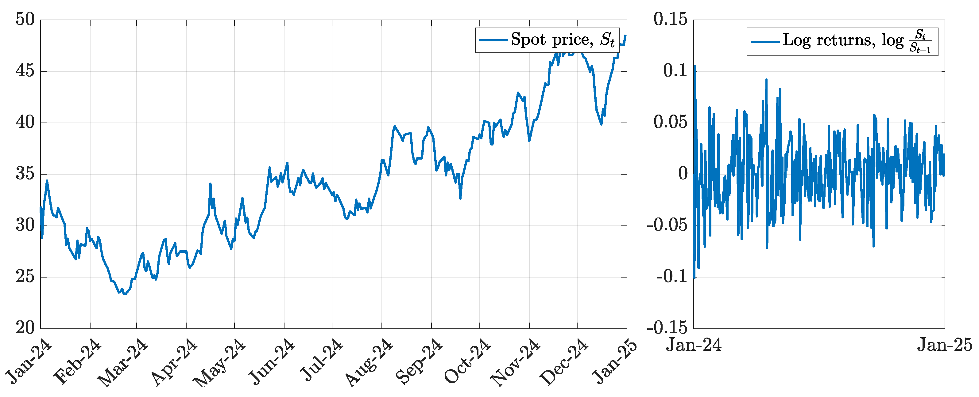
Following standard practice in commodity markets, we use the settlement price of the one-day-ahead futures contract on day t as a proxy for the natural gas spot price, denoted by $S_t$.

The left panel of Figure 1 illustrates the evolution of the natural gas spot price over 2024, comprising 262 daily observations. The right panel of the same figure presents the corresponding log returns, computed as $\log {\displaystyle \frac{S_t}{S_{t-1}}}$. Over the past year, the natural gas market has experienced a sharp increase in price levels, largely driven by geopolitical uncertainties. Meanwhile, spot price returns exhibit occasional spikes and evidence of mild volatility clustering.

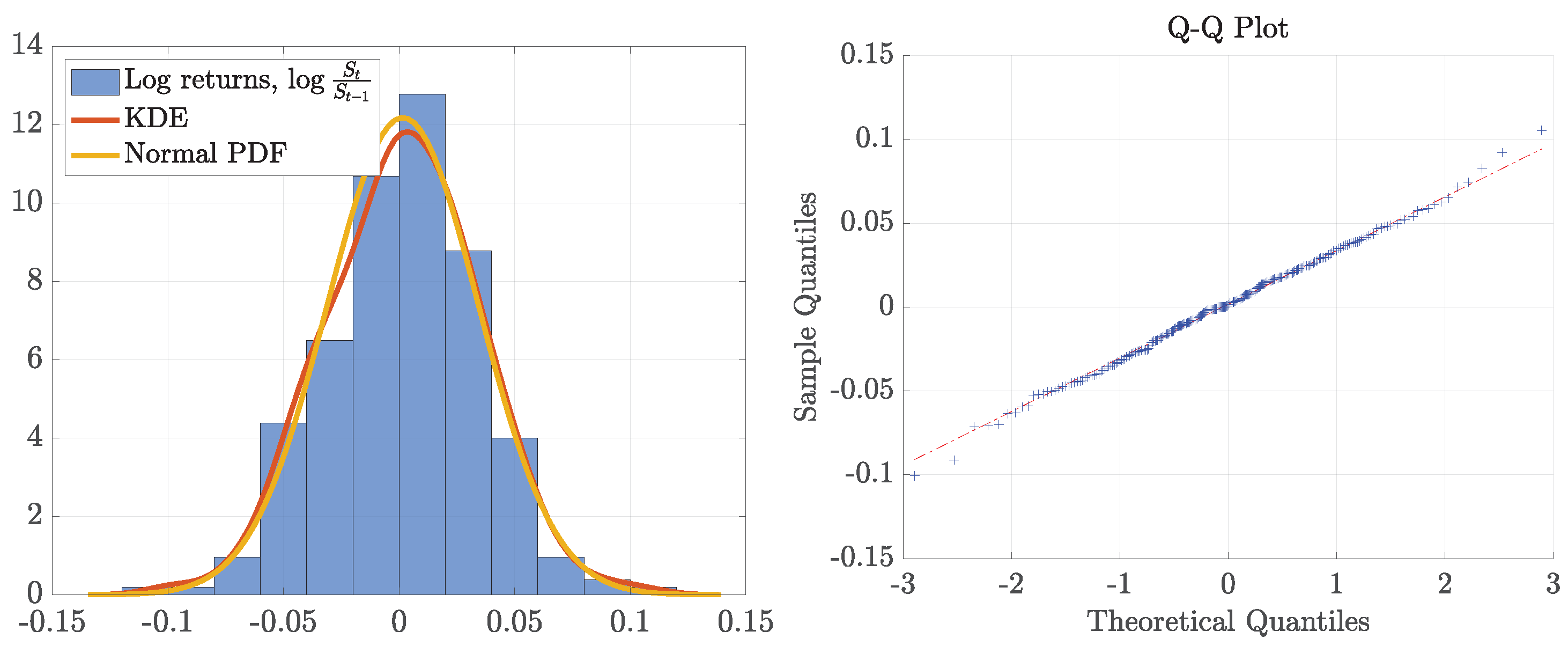
The left panel of Figure 2 shows the histogram of log returns, together with their kernel density estimate (KDE), benchmarked against the fitted normal density function. The right panel of the same figure displays the Q-Q plot of log returns. Overall, log returns have not deviated significantly from normality, as confirmed by the computation of their sample-centered moments: 0.0016 (mean), 0.0011 (variance), −0.0316 (skewness), and 3.1804 (kurtosis). The Jarque–Bera test does not reject the null hypothesis of normality, yielding a p-value greater than 0.5. However, the presence of a few outliers in the tails leads the Kolmogorov–Smirnov test to reject the same null hypothesis at any conventional significance level, with a p-value below 0.0001.

Therefore, while the normal distribution is not a perfect fit, as also shown by Gambaro and Secomandi (2021), it can serve here as a reasonable first-order approximation of natural gas returns. This supports the use of a seasonally adjusted version of the Gibson and Schwartz (1990) model, which assumes a lognormal distribution for the spot price $S_t$. As we will demonstrate, this assumption is not problematic when calibrating the forward curve but becomes inadequate when applied to option pricing.

2.2. Features of Futures Contracts

Futures contracts are traded at the TTF with maturities extending up to more than 150 consecutive months. Naturally, the most liquid contracts are those with maturities of less than two years, with particular emphasis on those expiring within one year. The pricing and contract size specifications of these futures closely resemble those of daily futures, as discussed in the previous subsection. Trading for these contracts concludes at the close of business two UK business days before the first calendar day of the delivery month.

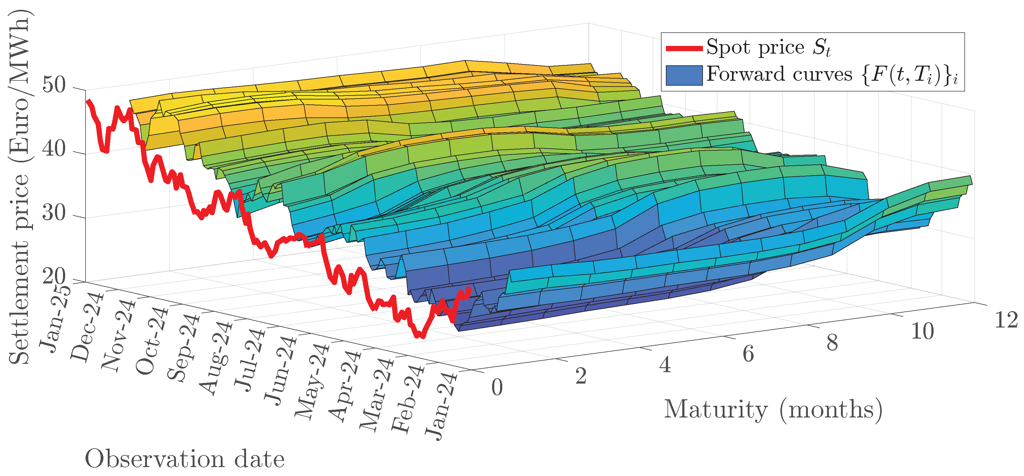
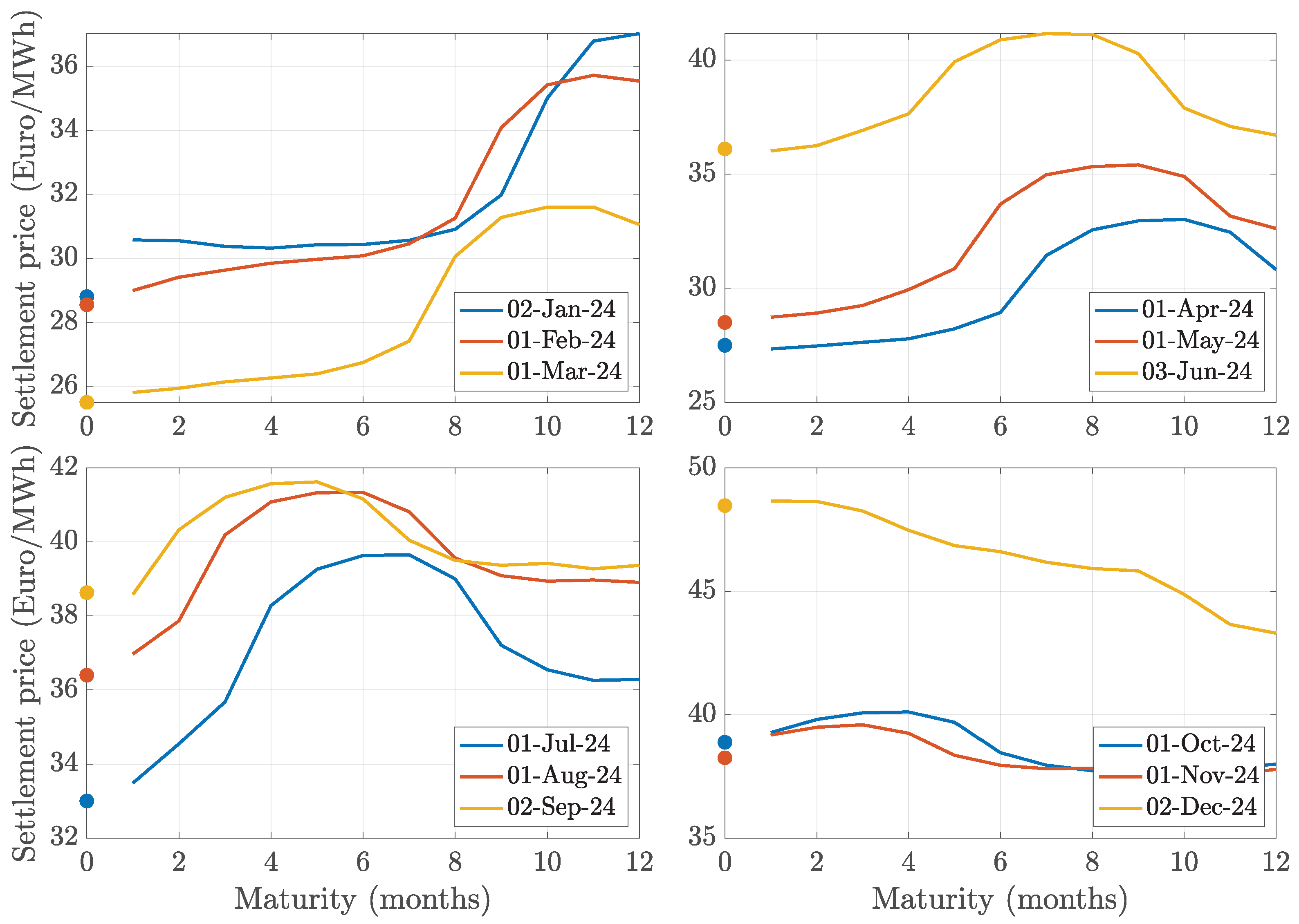
Following standard notation, we denote by $F(t,T)$ the settlement price on day t of a futures contract with delivery date T. At each day t, given a set of n maturities ${\left\{T_i\right\}}_{i=1}^n$, the collection of time-t futures prices for delivery dates $T_i$, denoted as ${\left\{F(t,T_i)\right\}}_{i=1}^n$, forms the so-called forward curve. Figure 3 illustrates the 12-month-ahead forward curves throughout 2024, representing the so-called forward surface, featuring 3144 daily prices. Additionally, Figure 4 presents presents the 12-month-ahead forward curves of natural gas for the first day of each month in 2024, grouped by quarter. Overall, the forward curves exhibit strong contango in the early months and leading into the summer, indicative of increasing demand expectations. The presence of backwardation in the third and fourth quarters suggests that market participants anticipate lower prices following peak demand periods. These patterns align with typical seasonal trends in natural gas markets, where prices tend to rise ahead of winter and summer before declining thereafter.

2.3. Features of Option Contracts

Options on natural gas futures are also actively traded at the TTF. In particular, European-style plain vanilla call and put options, available with a wide range of strike prices, are traded on each monthly futures contract, with maturities coinciding with the respective futures contract’s delivery date. If an option is not manually abandoned, in-the-money options are exercised automatically, resulting in the delivery of the underlying futures contract.

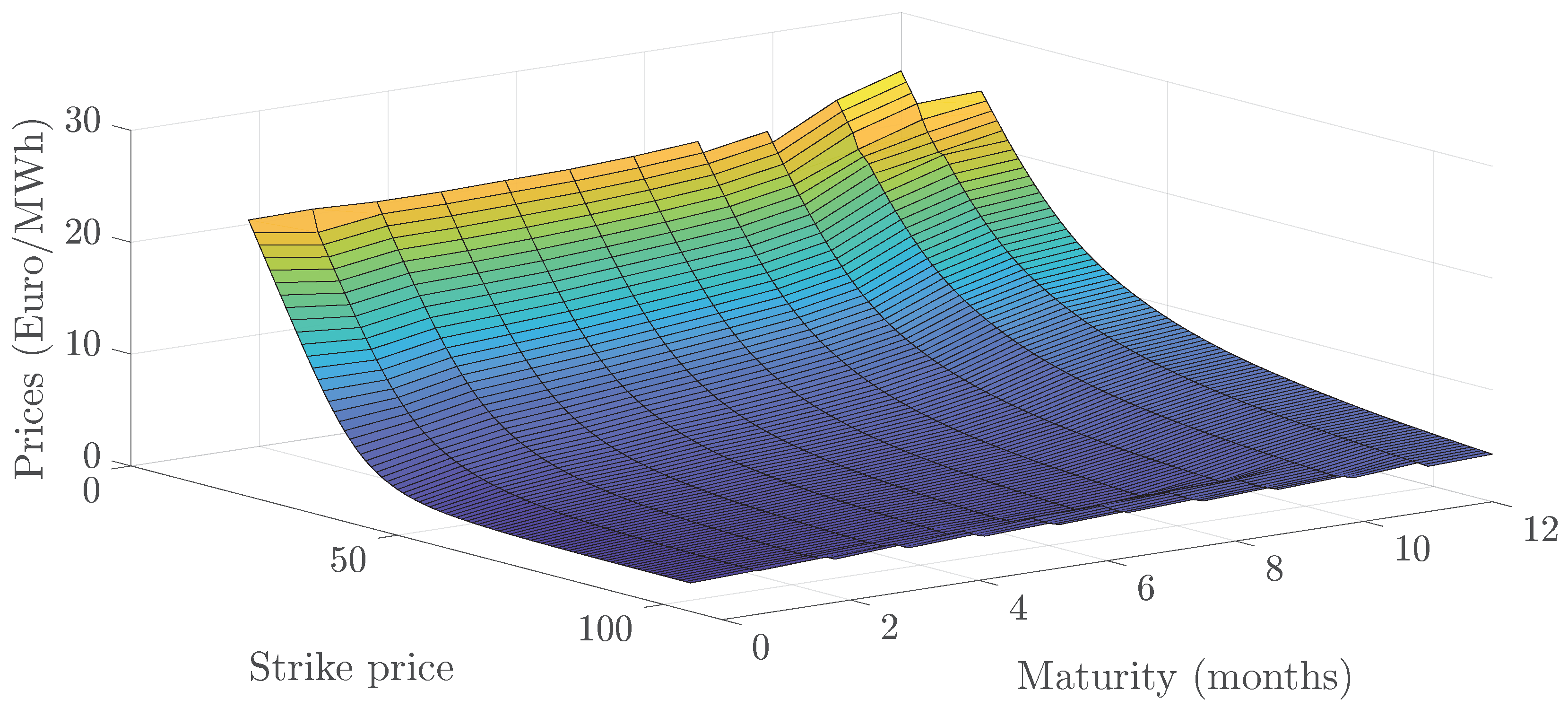
Figure 5 presents the entire price surface for call options as of the first trading day of 2024 for futures contracts with maturities extending up to twelve months. The underlying forward curve is depicted in the top-left panel of Figure 4, which indicates that the spot price on that day was 28.8. Furthermore, the futures market exhibited contango, characterized by an upward slope, reflecting market expectations of rising prices in the subsequent months following a period of stable prices. As expected, the price surface bends around the at-the-money level. The dataset generating the surface consists of 1050 individual points, with approximately 85 quoted strike prices per maturity, ranging from a minimum of 10 to a maximum of 110.

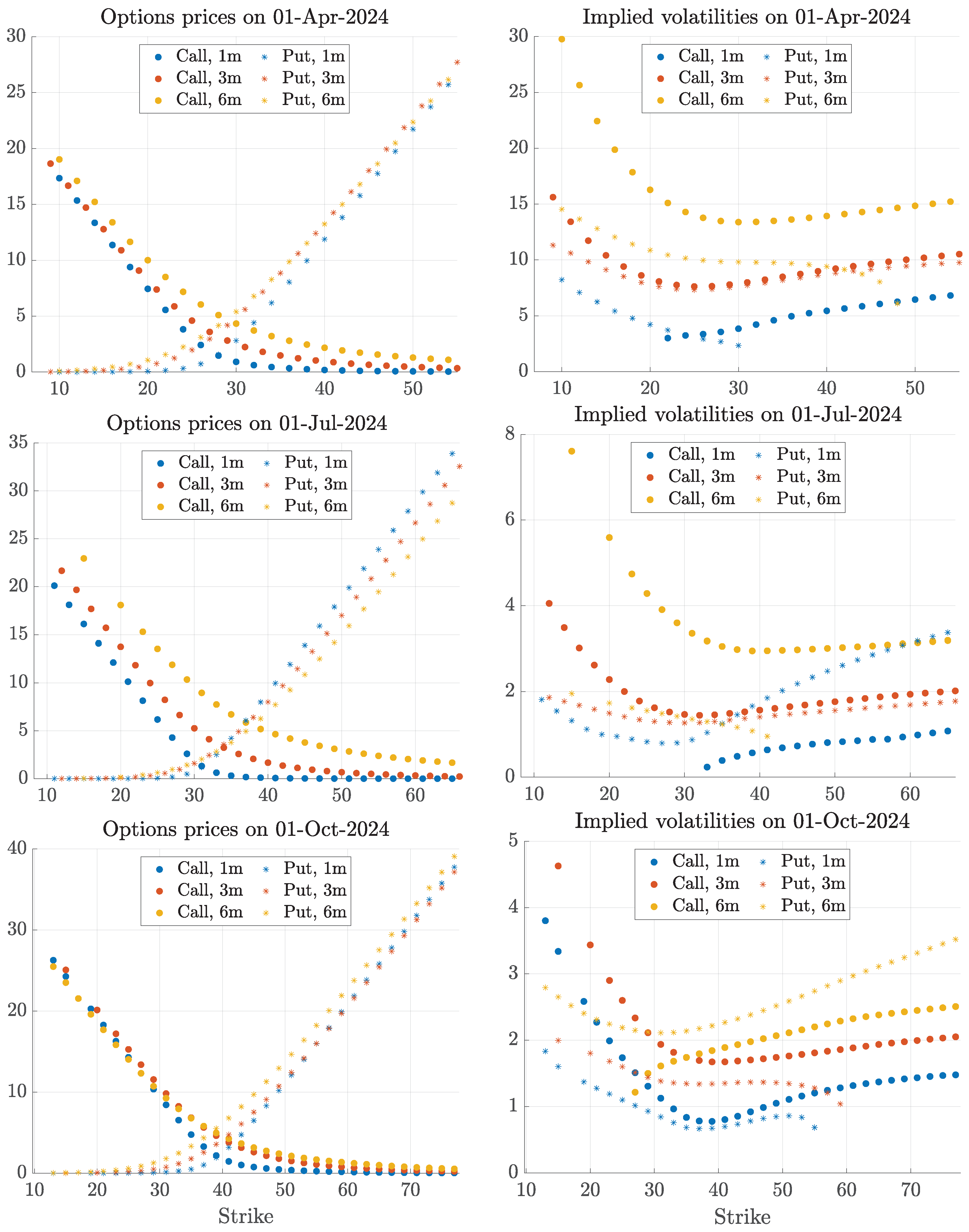
For brevity, the left panels of Figure 6 display the prices of call and put options with maturities of one, three, and six months on the first trading day of the remaining three quarters of 2024. Interestingly, these price curves are not always monotonic with respect to maturity, reflecting the seasonal patterns of natural gas demand and supply. For instance, on 1 July, call options on futures expiring in six months (i.e., at the end of December) are the most expensive among the displayed options, aligning with the peak of the blue forward curve in the bottom-left panel of Figure 4, which corresponds to the seasonal increase in demand during the colder months. Conversely, on 1 October, call options expiring in six months (i.e., at the end of March 2025) appear to be cheaper than those with shorter maturities. This behavior is consistent with the decline observed in the blue forward curve in the bottom-right panel of Figure 4, which corresponds to the seasonal reduction in natural gas demand during spring, a period characterized by minimal heating or cooling requirements.

Finally, the right panels of Figure 6 translate the price data from the left panels into Black-Scholes implied volatilities. As shown, the implied volatilities exhibit irregular patterns and reach extreme values, significantly deviating from the annualized sample historical standard deviation of the log returns of the spot price series, which is estimated at 0.5301. This observation suggests that a simple constant-volatility model is inadequate for capturing the distinctive behavior of natural gas options, as noted in the previous literature. Consequently, in the following section, we extend a seasonal version of the model proposed by Gibson and Schwartz (1990), which is effective for futures prices alone, by incorporating a local volatility factor to achieve a better fit for option prices as well.

As discussed in the preceding three subsections, natural gas financial contracts exhibit several distinctive characteristics, most notably a pronounced seasonality in forward curves and noticeable volatility smirks in option prices. While the latter is relatively common among commodity options, as evidenced by the extensive literature on the modeling of volatility structures in such markets (a concise summary of which is provided in Fanelli and Frau (2024)), the former is more specific to certain commodities. 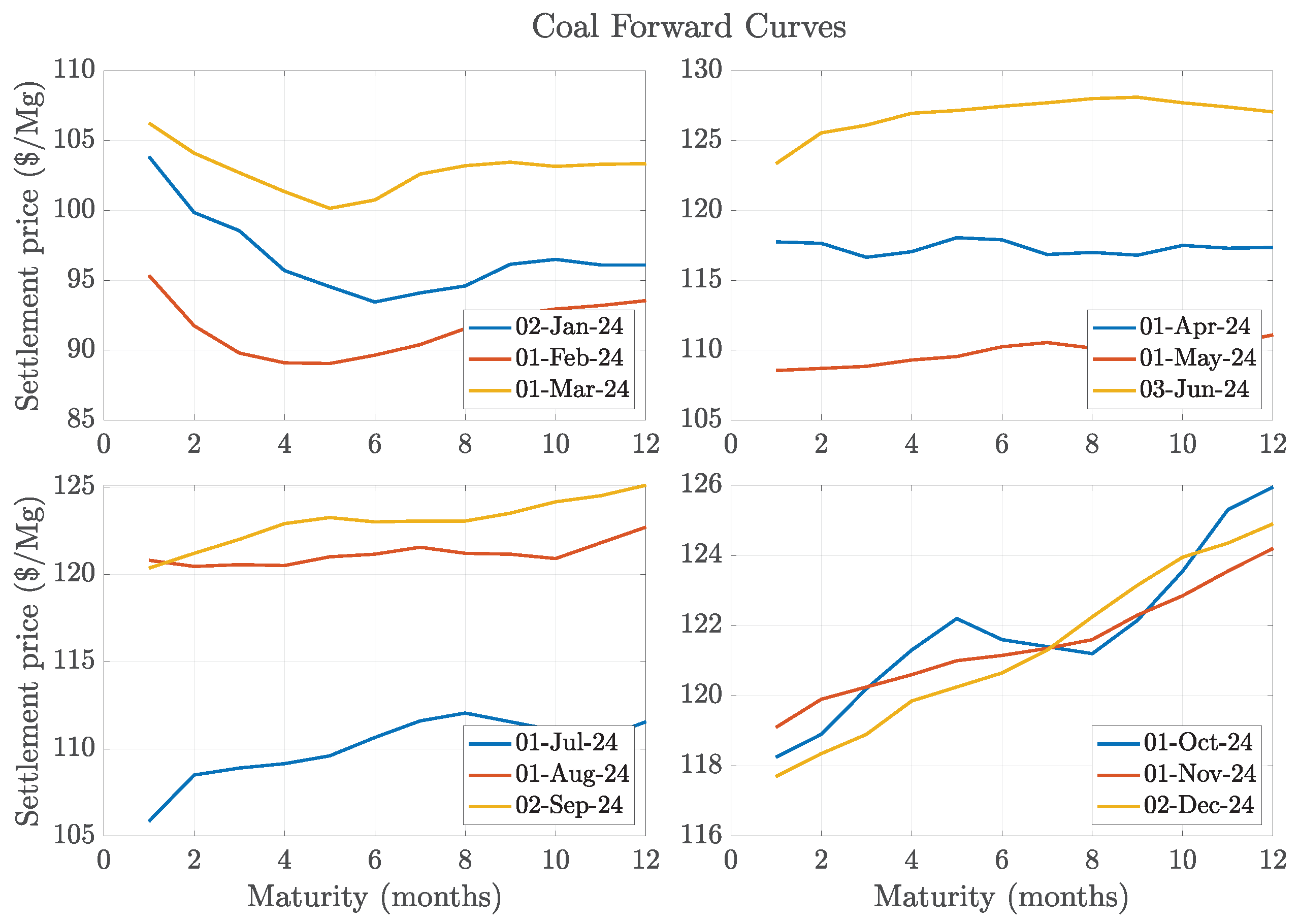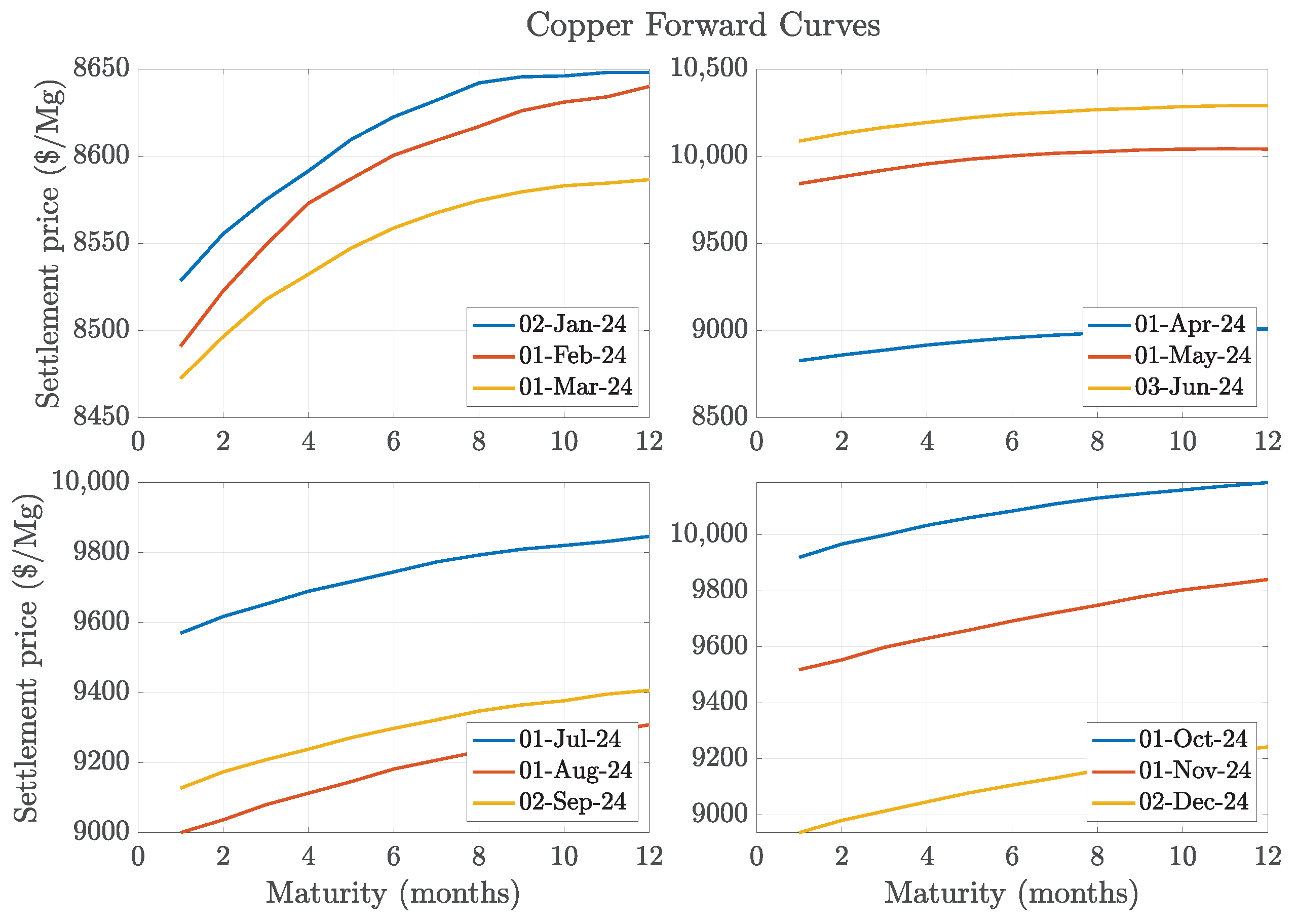Appendix A.2 presents the 12-month-ahead forward curves for four representative commodities, following the same approach as in Figure 4. As shown, coal and corn exhibit clear seasonal patterns, whereas copper and crude oil do not. This explains why the original model proposed by Gibson and Schwartz (1990), which is tailored to crude oil financial contracts, does not include a seasonal component—a limitation that becomes evident when modeling natural gas, where such a term is essential (see Remark 2).

3. The Local Volatility-Seasonal Stochastic Convenience Yield Model

In this section, we introduce two benchmark models for the natural gas spot market and discuss the methodology for pricing futures and options under both frameworks. Specifically, in Section 3.1, we present the seasonal convenience yield model, an extension of the seminal framework proposed by Gibson and Schwartz (1990). This model incorporates a seasonal component in the convenience yield to better capture the seasonality observed for futures prices in Section 2.2. In Section 3.2, we further extend this model by introducing a local volatility factor in the spot price process.

3.1. The Seasonal Stochastic Convenience Yield Model

We consider a frictionless, arbitrage-free financial market modeled by a filtered probability space $(\mathrm{\Omega },\mathcal{F},\mathbb{F}={\left({\mathcal{F}}_t\right)}_{t\ge 0},\mathbb{Q})$, which supports all the relevant stochastic processes introduced below. Here, $\mathbb{Q}$ denotes an equivalent martingale measure.

The market is assumed to have a deterministic term structure, with $r\left(t\right)$ representing the instantaneous risk-free interest rate. In the empirical analysis of the following section, $r\left(t\right)$ is modeled using the deterministic specification proposed by Svensson (1994)4.

Let $S={\left(S_t\right)}_{t\ge 0}$ denote the spot price of natural gas, and let $B={\left(B_t\right)}_{t\ge 0}$ represent the price process of the money market account, given by $B_t=\exp \left({\int }_0^{t}r\left(s\right)\mathrm{d}s\right)$. Furthermore, let $\delta ={\left({\delta }_t\right)}_{t\ge 0}$ denote the stochastic convenience yield associated with S.

Building on the seminal work of Gibson and Schwartz (1990), we assume that the convenience yield process $\delta$ consists of the sum of a deterministic seasonal component, represented by a periodic function $g\left(t\right)$, and a mean-reverting Ornstein–Uhlenbeck $x={\left(x_t\right)}_{t\ge 0}$. We subsequently refer to this model as the seasonal convenience yield model (sCY).

Formally, the sCY model is characterized by the following system of stochastic differential equations:

$$\begin{array}{cc}\hfill {\displaystyle \frac{\mathrm{d}{S}_t}{S_t}}& =\left(r\left(t\right)-{\delta }_t\right)\mathrm{d}t+{\sigma }_S\mathrm{d}{W}_t^S,\hfill \end{array}$$

(1)

$$\begin{array}{cc}\hfill \mathrm{d}{\delta }_t& =g^{\prime }\left(t\right)\mathrm{d}t+\mathrm{d}{x}_t\hfill \end{array}$$

(2)

$$\begin{array}{cc}\hfill \mathrm{d}{x}_t& =\kappa \left(\theta -x_t\right)\mathrm{d}t+{\sigma }_x\mathrm{d}{W}_t^x,\hfill \end{array}$$

(3)

with initial conditions $S_0\in {\mathbb{R}}^{+}$, ${\delta }_0\in \mathbb{R}$ and $x_0={\delta }_0-g\left(0\right)$.

The model parameters and processes are as follows:

• $W^S={\left(W_t^S\right)}_{t\ge 0}$ and $W^x={\left(W_t^x\right)}_{t\ge 0}$ are two standard Brownian motions with correlation $\rho \in [-1,1]$, representing the sources of market risk and convenience yield risk, respectively;
• the function $g\left(t\right):{\mathbb{R}}^{+}\to \mathbb{R}$ captures seasonality and is assumed to follow one of the easiest5 specifications proposed by Harvey (1989):

  $$g\left(t\right)=a\cos \left(bt+c\right)$$

  (4)

  with $a,b,c\in \mathbb{R}$;
• the parameters ${\sigma }_S,{\sigma }_x\in {\mathbb{R}}^{+}$ represent the volatilities of the spot price and of the mean-reverting component of the convenience yield, while $\kappa ,\theta \in \mathbb{R}$ denote the speed of mean reversion and the long-run mean of the latter.

Remark 1. 

It is worth noting that if the seasonal component is removed by setting $g(·)\equiv 0$, the sCY model reduces to the original model proposed by Gibson and Schwartz (1990) for financial contracts based on crude oil futures.

3.1.1. Solution of the sCY Model

We now look for (conditional) solutions to the SDEs in (1)–(3).

Starting from x it is known that, conditional of t,

$$x_T=x_t{e}^{-\kappa (T-t)}+\theta \left(1-e^{-\kappa (T-t)}\right)+{\sigma }_x{\int }_t^T{e}^{-\kappa (T-u)}\mathrm{d}{W}_u^x$$

for any $T\ge t$. As for S, the stochastic differential of $\ln S_t$ computed by Itô’s Formula6 delivers

$$\begin{array}{cc}\hfill \mathrm{d}\ln S_t=& {\displaystyle \frac{1}{S_t}}\mathrm{d}{S}_t-{\displaystyle \frac{1}{2}}{\displaystyle \frac{1}{S_t^2}}\mathrm{d}{\langle {\sigma }_S{S}_t{W}^S,{\sigma }_S{S}_t{W}^S\rangle }_t\hfill \\ \hfill =& {\displaystyle \frac{1}{S_t}}\left(S_t\left(r\left(t\right)-{\delta }_t\right)\mathrm{d}t+{\sigma }_S{S}_t\mathrm{d}{W}_t^S\right)-{\displaystyle \frac{1}{2}}{\displaystyle \frac{1}{S_t^2}}{\sigma }_S^2{S}_t^2\mathrm{d}t\hfill \\ \hfill =& \left(r\left(t\right)-{\delta }_t-{\displaystyle \frac{{\sigma }_S^2}{2}}\right)\mathrm{d}t+{\sigma }_S\mathrm{d}{W}_t^S.\hfill \end{array}$$

Integrating from t to T delivers

$$\ln S_T-\ln S_t={\int }_t^T\left(r\left(s\right)-{\delta }_s-{\displaystyle \frac{{\sigma }_S^2}{2}}\right)\mathrm{d}s+{\sigma }_S{\int }_t^T\mathrm{d}{W}_s^S.$$

Taking exponentials and rearranging terms, we find that, conditional on t,

$$S_T=S_t\exp \left({\int }_t^T\left(r\left(s\right)-{\delta }_s\right)\mathrm{d}s-{\displaystyle \frac{{\sigma }_S^2}{2}}\left(T-t\right)+{\sigma }_S\left(W_T^S-W_t^S\right)\right).$$

Since (2) simply solves as ${\delta }_t=g\left(t\right)+x_t$, separating the deterministic components from the stochastic ones, we obtain

$$\begin{array}{cc}\hfill S_T& =S_t\exp \left({\int }_t^T\left(r\left(s\right)-g\left(s\right)-x_s\right)\mathrm{d}s-{\displaystyle \frac{{\sigma }_S^2}{2}}\left(T-t\right)\right)\exp \left({\sigma }_S\left(W_T^S-W_t^S\right)\right)\hfill \\ \hfill & =S_t\exp \left({\int }_t^T\left(r\left(s\right)-g\left(s\right)\right)\mathrm{d}s-{\int }_t^T\left(x_t{e}^{-\kappa (s-t)}+\theta \left(1-e^{-\kappa (s-t)}\right)\right)\mathrm{d}s-{\displaystyle \frac{{\sigma }_S^2}{2}}\left(T-t\right)\right)·\hfill \\ \hfill & ·\exp \left(-{\sigma }_x{\int }_t^T\left({\int }_t^s{e}^{-\kappa (s-u)}\mathrm{d}{W}_u^x\right)\mathrm{d}s+{\sigma }_S\left(W_T^S-W_t^S\right)\right).\hfill \end{array}$$

Setting $B(t,T):={\displaystyle \frac{1}{\kappa }}\left(1-e^{-\kappa (T-t)}\right)$, we can write

$$\begin{array}{cc}\hfill S_T& =S_t\exp \left({\int }_t^T\left(r\left(s\right)-g\left(s\right)\right)\mathrm{d}s-x_{t}B(t,T)-\theta \left(T-t-B(t,T)\right)-{\displaystyle \frac{{\sigma }_S^2}{2}}\left(T-t\right)\right)·\hfill \\ \hfill & ·\exp \left(-{\sigma }_x{\int }_t^T\left({\int }_t^s{e}^{-\kappa (s-u)}\mathrm{d}{W}_u^x\right)\mathrm{d}s+{\sigma }_S\left(W_T^S-W_t^S\right)\right).\hfill \end{array}$$

Notice that, since the argument of the double integral in the last exponential is strictly positive, thanks to the Fubini’s Theorem for stochastic integrals (see Result 6.12 in Karatzas and Shreve 1998), we can also write

$$\begin{array}{cc}\hfill {\int }_t^T\left({\int }_t^s{e}^{-\kappa (s-u)}\mathrm{d}{W}_u^x\right)\mathrm{d}s& ={\int }_t^T\left({\int }_u^T{e}^{-\kappa (s-u)}\mathrm{d}s\right)\mathrm{d}{W}_u^x\hfill \\ \hfill & ={\int }_t^{T}B(u,T)\mathrm{d}{W}_u^x.\hfill \end{array}$$

Therefore, setting $A(t,T):={\int }_t^T\left(r\left(s\right)-g\left(s\right)\right)\mathrm{d}s-\theta \left(T-t-B(t,T)\right)-{\displaystyle \frac{{\sigma }_S^2}{2}}\left(T-t\right)$, we have

$$S_T=S_t\exp \left(A(t,T)-x_{t}B(t,T)\right)\exp \left(-{\sigma }_x{\int }_t^{T}B(u,T)\mathrm{d}{W}_u^x+{\sigma }_S\left(W_T^S-W_t^S\right)\right).$$

(5)

Notice that $\left(W_T^S-W_t^S\right)$ can be rewritten as ${\int }_t^T\mathrm{d}{W}_u^S$. As the exponential in (5) is involving two stochastic integrals of deterministic functions of time, their sum is normally distributed with zero expected value and variance equal to

$$\begin{array}{cc}\hfill C^2(t,T)& :=V\left[-{\sigma }_x{\int }_t^{T}B(u,T)\mathrm{d}{W}_u^x+{\sigma }_S{\int }_t^T\mathrm{d}{W}_u^S\right]\hfill \\ \hfill & =V\left[{\sigma }_x{\int }_t^{T}B(u,T)\mathrm{d}{W}_u^x\right]+V\left[{\sigma }_S{\int }_t^T\mathrm{d}{W}_u^S\right]-2Cov\left[{\sigma }_x{\int }_t^{T}B(u,T)\mathrm{d}{W}_u^x,{\sigma }_S{\int }_t^T\mathrm{d}{W}_u^S\right].\hfill \end{array}$$

Recalling that $\mathrm{d}{〈W^x,W^S〉}_u=\rho \mathrm{d}u$, thanks to Itô’s Isometry, we get

$$\begin{array}{cc}\hfill C^2(t,T)& ={\sigma }_x^2{\int }_t^T{B}^2(u,T)\mathrm{d}u+{\sigma }_S^2{\int }_t^T\mathrm{d}u-2{\sigma }_x{\sigma }_S{\int }_t^{T}B(u,T)\rho \mathrm{d}u\hfill \\ \hfill & ={\displaystyle \frac{{\sigma }_x^2}{2{\kappa }^3}}\left(-3+4e^{-\kappa \left(T-t\right)}-e^{-2\kappa (T-t)}+2\kappa \left(T-t\right)\right)+{\sigma }_S^2\left(T-t\right)+\hfill \\ \hfill & -{\displaystyle \frac{2{\sigma }_x{\sigma }_S\rho }{{\kappa }^2}}\left(-1+e^{-\kappa \left(T-t\right)}+\kappa (T-t)\right).\hfill \end{array}$$

Therefore, conditional on t, it holds

$$\log S_T\sim \mathcal{N}\left(\log S_t+A(t,T)-x_{t}B(t,T),C^2(t,T)\right).$$

(6)

3.1.2. Pricing Within the sCY Model

We now look for both futures and options prices within the sCY model.

Since there is no interest rate risk, the t-price $F(t,T)$ of a futures contract on S with delivery T can be simply computed as $F(t,T)=\mathbb{E}\left[\left.S_T\right|{\mathcal{F}}_t\right]$7. Using the distributional result in (6), we have

$$\begin{array}{cc}\hfill F(t,T)& =\mathbb{E}\left[\left.S_T\right|{\mathcal{F}}_t\right]=\exp \left(\log S_t+A(t,T)-x_{t}B(t,T)+{\displaystyle \frac{C^2(t,T)}{2}}\right)\hfill \\ \hfill & =S_t\exp \left({\int }_t^T\left(r\left(s\right)-g\left(s\right)\right)\mathrm{d}s-\theta \left(T-t-B(t,T)\right)-x_{t}B(t,T)+\right.\hfill \\ \hfill & \left.+{\displaystyle \frac{{\sigma }_x^2}{4{\kappa }^3}}\left(-3+4e^{-\kappa \left(T-t\right)}-e^{-2\kappa (T-t)}+2\kappa \left(T-t\right)\right)-{\displaystyle \frac{{\sigma }_x{\sigma }_S\rho }{{\kappa }^2}}\left(-1+e^{-\kappa \left(T-t\right)}+\kappa (T-t)\right)\right).\hfill \\ \hfill & =S_t\exp \left({\int }_t^T\left(r\left(s\right)-g\left(s\right)\right)\mathrm{d}s-x_{t}B(t,T)+{\displaystyle \frac{{\sigma }_x^2}{4{\kappa }^3}}\left(-3+4e^{-\kappa \left(T-t\right)}-e^{-2\kappa (T-t)}+2\kappa \left(T-t\right)\right)+\right.\hfill \\ \hfill & +\left.{\displaystyle \frac{\kappa \theta +{\sigma }_x{\sigma }_S\rho }{\kappa }}\left(B(t,T)-(T-t)\right)\right).\hfill \end{array}$$

(7)

Moreover, given and the explicit choice of $g\left(·\right)$ in (4), we also have

$$\begin{array}{cc}\hfill \exp \left({\int }_t^T\left(r\left(s\right)-g\left(s\right)\right)\mathrm{d}s\right)& =\exp \left({\int }_t^T\left(r\left(s\right)-g\left(s\right)\right)\mathrm{d}s\right)\hfill \\ \hfill & =\exp \left(y\left(T\right)T-y\left(t\right)t-{\displaystyle \frac{a}{b}}\left(\sin \left(bT+c\right)-\sin \left(bt+c\right)\right)\right)\hfill \end{array}$$

where $y(·)$ is the yield to maturity8 of the riskless security.

As it will be particularly useful later on, the unconditional time-0 futures price within the sCY model, $F^{sCY}(0,T)$, of a futures contract on S with maturity T is given by

$$\begin{array}{cc}\hfill F^{sCY}(0,T)& =S_0\exp \left(y\left(T\right)T-{\displaystyle \frac{a}{b}}\left(\sin \left(bT+c\right)-\sin \left(c\right)\right)-x_{0}B(0,T)+\right.\hfill \\ \hfill & \left.+{\displaystyle \frac{{\sigma }_x^2}{4{\kappa }^3}}\left(-3+4e^{-\kappa T}-e^{-2\kappa T}+2\kappa T\right)+{\displaystyle \frac{\kappa \theta +{\sigma }_x{\sigma }_S\rho }{\kappa }}\left(B(0,T)-T\right)\right).\hfill \end{array}$$

(8)

Remark 2. 

The explicit futures price formula in the original model of Gibson and Schwartz (1990) can be derived from Equation (7) by setting $g(·)\equiv 0$ (see Remark 1). In this case, the argument of the exponential leads to forward curves $F(t,T)$ characterized by a single peak and at most one inflection point. This makes it evident that the inclusion of the seasonal component g in the convenience yield is essential to reproduce the wavy shapes observed in the forward curves shown in Figure 4, and even more so in the left panels of Figure 7 and Figure 8.

We now turn to option pricing. As recalled in Section 2.3, in the natural gas market, options are written on futures contracts. In order to derive the closed-form solution for the price of European call and put options on futures contracts, we first need to study their price process evolution. From (7), we can write $F(t,T)$ as

$$F(t,T)=S_t\exp \left(A(t,T)-x_{t}B(t,T)+{\displaystyle \frac{C^2(t,T)}{2}}\right).$$

Taking the stochastic differential of $F(t,T)$ according to Itô’s formula, we obtain

$$\begin{array}{cc}\hfill {\displaystyle \frac{\mathrm{d}F(t,T)}{F(t,T)}}& =\left(A^{\prime }(t,T)-x_t{B}^{\prime }(t,T)+C(t,T)C^{\prime }(t,T)\right)\mathrm{d}t+{\displaystyle \frac{1}{S_t}}\mathrm{d}{S}_t-B(t,T)\mathrm{d}{x}_t+\hfill \\ \hfill & +{\displaystyle \frac{1}{2}}{B}^2(t,T)\mathrm{d}{〈x,x〉}_t-{\displaystyle \frac{B(t,T)}{S_t}}\mathrm{d}{〈x,S〉}_t\hfill \\ \hfill & =\left(A^{\prime }(t,T)-x_t{B}^{\prime }(t,T)+C(t,T)C^{\prime }(t,T)\right)\mathrm{d}t+\left(r\left(t\right)-g\left(t\right)-x_t\right)\mathrm{d}t+{\sigma }_S\mathrm{d}{W}_t^S+\hfill \\ \hfill & -B(t,T)\left(\kappa \left(\theta -x_t\right)\mathrm{d}t+{\sigma }_x\mathrm{d}{W}_t^x\right)+{\displaystyle \frac{{\sigma }_x^2}{2}}{B}^2(t,T)\mathrm{d}t-B(t,T){\sigma }_S{\sigma }_x\rho \mathrm{d}t\hfill \\ \hfill & =\left(\dots \right)\mathrm{d}t+{\sigma }_S\mathrm{d}{W}_t^S-B(t,T){\sigma }_x\mathrm{d}{W}_t^x.\hfill \end{array}$$

(9)

As $F(t,T)=\mathbb{E}\left[\left.S_T\right|{\mathcal{F}}_t\right]$, $F(t,T)$ must be a martingale. Therefore, the drift in (9) has to be equal to zero so that

$${\displaystyle \frac{\mathrm{d}F(t,T)}{F(t,T)}}={\sigma }_S\mathrm{d}{W}_t^S-B(t,T){\sigma }_x\mathrm{d}{W}_t^x,$$

which is indeed a stochastic exponential.

As a consequence, for any $t>v$,

$$\begin{array}{cc}\hfill F(t,T)& =F(v,T)\exp \left(-{\displaystyle \frac{1}{2}}{\int }_v^t\left({\sigma }_S^2+B^2(u,T){\sigma }_x^2+B(u,T){\sigma }_S{\sigma }_x\rho \right)\mathrm{d}u+\right.\hfill \\ \hfill & \left.+{\sigma }_S{\int }_v^t\mathrm{d}{W}_u^S-{\sigma }_x{\int }_v^{t}B(u,T)\mathrm{d}{W}_u^x\right)\hfill \\ \hfill & =F(v,T)\exp \left(-{\displaystyle \frac{C{(v,t)}^2}{2}}+{\sigma }_S{\int }_v^t\mathrm{d}{W}_u^S-{\sigma }_x{\int }_v^{t}B(u,T)\mathrm{d}{W}_u^x\right).\hfill \end{array}$$

From a distributional point of view, conditional on v,

$$\log F(t,T)\sim \mathcal{N}\left(\log F(v,T)-{\displaystyle \frac{C^2(v,t)}{2}},C^2(v,t)\right).$$

This explicit characterization allows for generalizing the seminal formula by Black (1976) and computing $c\left(t\right)$, the time-t price of a call option on the futures contract with delivery date and maturity T and strike price K when the futures contract quotes $F(t,T)$. In particular, we have

$$\begin{array}{cc}\hfill c\left(t\right)& =\mathbb{E}\left[\left.e^{-{\int }_t^{T}r\left(s\right)\mathrm{d}s}{\left(F(T,T)-K\right)}^{+}\right|{\mathcal{F}}_t\right]\hfill \\ \hfill & =e^{-{\int }_t^{T}r\left(s\right)\mathrm{d}s}\left(\mathbb{E}\left[\left.F(T,T){\mathbb{I}}_{F(T,T)\ge K}\right|{\mathcal{F}}_t\right]-K\mathbb{Q}\left[\left.F(T,T)\ge K\right|{\mathcal{F}}_t\right]\right)\hfill \\ \hfill & =e^{-{\int }_t^{T}r\left(s\right)\mathrm{d}s}\left(F(t,T)N\left({\tilde{d}}_1(t,T)\right)-KN\left({\tilde{d}}_2(t,T)\right)\right)\hfill \end{array}$$

(10)

with

$${\tilde{d}}_1(t,T)={\displaystyle \frac{\log \frac{F(t,T)}{K}+\frac{C^2(t,T)}{2}}{\sqrt{C^2(t,T)}}}\mathrm{and}{\tilde{d}}_2(t,T)={\tilde{d}}_1(t,T)-\sqrt{C^2(t,T)}$$

(11)

and where $N(·)$ represents the cumulative distribution function of a standard normal random variable.

Following similar steps, it is possible to obtain the time-t price $p\left(t\right)$ of a put option on the futures contract with delivery date and maturity T, and strike price K when the futures contract quotes $F(t,T)$. Indeed,  

$$\begin{array}{cc}\hfill p\left(t\right)& =\mathbb{E}\left[\left.e^{-{\int }_t^{T}r\left(s\right)\mathrm{d}s}{\left(K-F(T,T)\right)}^{+}\right|{\mathcal{F}}_t\right]\hfill \\ \hfill & =e^{-{\int }_t^{T}r\left(s\right)\mathrm{d}s}\left(K\mathbb{Q}\left[\left.F(T,T)\le K\right|{\mathcal{F}}_t\right]-\mathbb{E}\left[\left.F(T,T){\mathbb{I}}_{F(T,T)\le K}\right|{\mathcal{F}}_t\right]\right)\hfill \\ \hfill & =e^{-{\int }_t^{T}r\left(s\right)\mathrm{d}s}\left(KN\left(-{\tilde{d}}_2(t,T)\right)-F(t,T)N\left(-{\tilde{d}}_1(t,T)\right)\right).\hfill \end{array}$$

(12)

where ${\tilde{d}}_1$ and ${\tilde{d}}_2$ are defined in (11).

For further reference, the unconditional time-0 prices of a call and a put option on the futures contract with delivery date and maturity T and strike price K within the sCY model are given by

$$\begin{array}{c}{c}^{sCY}\left(0\right)=e^{-y\left(T\right)T}\left(F(0,T)N\left({\tilde{d}}_1(0,T)\right)-KN\left({\tilde{d}}_2(0,T)\right)\right)\hfill \\ p^{sCY}\left(0\right)=e^{-y\left(T\right)T}\left(KN\left(-{\tilde{d}}_2(0,T)\right)-F(0,T)N\left(-{\tilde{d}}_1(0,T)\right)\right).\hfill \end{array}$$

(13)

3.2. The Local Volatility-Seasonal Stochastic Convenience Yield Model

We now extend the sCY model by incorporating a local volatility component inspired by the Constant Elasticity of Variance (CEV) model introduced by Cox (1975). This modification enables capturing the well-documented leverage effect, documented in energy markets also by Kristoufek (2014), without introducing an additional source of risk/Brownian motion, thereby preserving model parsimony.

This extension is expected to improve the fitting accuracy of the standard sCY model when applied to option pricing, producing return distributions that exhibit larger deviations from the normal benchmark, in terms of negative skewness and leptokurtic behaviour. These features are consistent with those of the spot price process, as analysed in Section 2.1. In the following, we refer to this alternative model as the Constant Elasticity of Variance—Seasonal Convenience Yield model (CEV-sCY).

Within the same framework as the sCY model presented in Section 3.1, we modify the stochastic differential equation governing the natural gas spot price S in (1) as follows:

$$\mathrm{d}{S}_t=S_t\left(r\left(t\right)-{\delta }_t\right)\mathrm{d}t+{\sigma }_S{S}_t^{\gamma }\mathrm{d}{W}_t^S,$$

(14)

where $\gamma \in {\mathbb{R}}^{+}$ represents the elasticity of variance, while all other processes and parameters remain consistent with those in the sCY model.

Unlike the sCY model, for which an explicit solution was derived in Section 3.1.1, the CEV-sCY model does not admit a closed-form solution. Therefore, in the next subsection, we introduce a flexible and computationally feasible lattice discretization of the CEV-sCY model that enables the pricing of both futures and options by the standard backward recursion introduced together with the binomial tree by Cox et al. (1979).

For completeness, we note that explicit pricing formulas can be derived within the CEV framework when the convenience yield is deterministic. Specifically, if the convenience yield consists solely of its deterministic seasonal component, i.e., ${\delta }_t=g\left(t\right)$, the spot price follows a complementary non-central chi-square distribution featuring an explicit, yet not straightforward, density function (for early work on option pricing within the CEV model, see Emanuel and MacBeth (1982), and for a comprehensive comparison of numerical techniques applicable to the CEV model, refer to Larguinho et al. (2013)).

A Lattice Representation for the CEV-sCY Model

The construction of a bivariate lattice representation for the CEV-sCY model follows a similar approach to the one used for the two-factor stochastic interest rate model discussed in detail by Battauz and Rotondi (2022).

Let $W^X={\left(W_t^X\right)}_{t\ge 0}$ and $W^Y={\left(W_t^Y\right)}_{t\ge 0}$ be two standard Brownian motions with instantaneous correlation $\rho \in [-1,1]$. As outlined in Stroock and Varadhan (1997), a general bivariate stochastic process ${\left\{(X_t,Y_t)\right\}}_{t\ge 0}$, defined by

$$\left\{\begin{array}{c}\mathrm{d}{X}_t={\mu }_X\mathrm{d}t+{\sigma }_X\mathrm{d}{W}_t^X\hfill \\ \mathrm{d}{Y}_t={\mu }_Y\mathrm{d}t+{\sigma }_Y\mathrm{d}{W}_t^Y\hfill \end{array}\right.$$

(15)

with initial conditions $X_0,Y_0\in \mathbb{R}$, where the drift terms ${\mu }_X$ and ${\mu }_Y$ may depend on t, $X_t$, and $Y_t$, admits a feasible lattice discretization (whose details are recalled in the Appendix A), provided that ${\sigma }_X$ and ${\sigma }_Y$ are positive constants.

In the context of the CEV-sCY model, the stochastic differential equations to be discretized are

$$\left\{\begin{array}{c}\mathrm{d}{S}_t=S_t\left(r\left(t\right)-{\delta }_t\right)\mathrm{d}t+{\sigma }_S{S}_t^{\gamma }\mathrm{d}{W}_t^S\hfill \\ \mathrm{d}{\delta }_t=g^{\prime }\left(t\right)\mathrm{d}t+\kappa \left(\theta -x_t\right)\mathrm{d}t+{\sigma }_x\mathrm{d}{W}_t^x\hfill \end{array}\right.$$

(16)

where the presence of the local volatility term in S prevents direct application of a standard lattice discretization due to the non-constant diffusion coefficient. However, following the approach of Rotondi (2024a), we first discretize the transformed process $\left(f\right(S),\delta )$, where f is a suitable function ensuring a constant diffusive term in $\mathrm{d}f\left(S\right(t\left)\right)$. Then, the discretization of the original S can then be retrieved through the inverse transformation $f^{-1}(·)$.

Applying Itô’s lemma to $X_t:={\displaystyle \frac{S_t^{1-\gamma }}{1-\gamma }}$ yields

$$\mathrm{d}{X}_t=\left((1-\gamma )X_t(r\left(t\right)-{\delta }_t)-{\displaystyle \frac{{\sigma }_S^2}{2}}{\displaystyle \frac{\gamma }{1-\gamma }}{\displaystyle \frac{1}{X_t}}\right)\mathrm{d}t+{\sigma }_S\mathrm{d}{W}_t^S.$$

Thus, the bivariate stochastic process $(X,Y)=\left({\displaystyle \frac{S^{1-\gamma }}{1-\gamma }},\delta \right)$ satisfies (15) with

$${\mu }_X=(1-\gamma )X(r-Y)-{\displaystyle \frac{{\sigma }_S^2}{2}}{\displaystyle \frac{\gamma }{1-\gamma }}{\displaystyle \frac{1}{X}},{\mu }_Y=g^{\prime }\left(t\right)+\kappa (\theta -Y),{\sigma }_X={\sigma }_S,{\sigma }_Y={\sigma }_x,$$

where the initial conditions are given by $X_0={\displaystyle \frac{S_0^{1-\gamma }}{1-\gamma }}$ and $Y_0={\delta }_0$.

Consequently, we can efficiently discretize the transformed pair $\left({\displaystyle \frac{S^{1-\gamma }}{1-\gamma }},\delta \right)$ using a computationally feasible bivariate lattice and recover the discretized values of S by inverting the definition of $X_t$, specifically setting $S_t={\left((1-\gamma )X_t\right)}^{{\displaystyle \frac{1}{1-\gamma }}}$.

Let ${\rm Y}={\{i\Delta t\}}_{i=0}^n$ be an n-step uniform partition of the interval $[0,T]$, where $\Delta t:={\displaystyle \frac{T}{n}}$. Consider the n-step computationally feasible lattice discretization of the CEV-sCY model described above, denoted by ${\left\{({\widehat{S}}_{t_i},{\widehat{\delta }}_{t_i})\right\}}_{t_i\in {\rm Y}}$.

Let $\phi (·)$ be a generic payoff function. The initial no-arbitrage price of a contingent claim with a time-T payoff $\phi \left(S_T\right)$ within the discretized CEV-sCY model is given by ${\widehat{V}}_{t_0}^{\phi }$. This value is computed using the standard backward recursion

$$\left\{\begin{array}{cc}{\widehat{V}}_{t_n}^{\phi }={\widehat{S}}_{t_n}\hfill & \\ {\widehat{V}}_{t_i}^{\phi }=e^{-y\left(t_{i+1}\right)t_{i+1}+y\left(t_i\right)t_i}\mathbb{E}\left[\left.{\widehat{V}}_{t_{i+1}}^{\phi }\right|{\mathcal{F}}_{t_i}\right]\hfill & \mathrm{for}i=n-1,\dots ,0,\hfill \end{array}\right.$$

(17)

where $y\left(t\right)$ represents the yield to maturity on the riskless security, whose explicit expression is provided in Note 8.

In particular, the unconditional time-0 futures price $F^{CEV-sCY}(0,T)$ of a futures contract on S with maturity T within the CEV-sCY model is obtained by setting $\phi \left(x\right)=x$. Furthermore, the unconditional time-0 prices of a call and a put option on the futures contract within the same model, with delivery date and maturity T and strike price K, denoted by $c^{CEV-sCY}\left(0\right)$ and $p^{CEV-sCY}\left(0\right)$, respectively, are determined by choosing $\phi \left(x\right)={(x-K)}^{+}$ for the call option and $\phi \left(x\right)={(K-x)}^{+}$ for the put option.

4. Empirical Analysis

In this section, we calibrate the two models introduced in the previous section to futures prices, evaluating both their in-sample fit, assessing how well the models capture the observed forward curves, and, more importantly, their out-of-sample performance in reproducing unseen data on options written on the same futures. Specifically, we first provide details of our calibration approach in Section 4.1; then, we conduct this calibration for the sCY model in Section 4.2 and for the CEV-sCY model in Section 4.3. Finally, in Section 4.4, we evaluate the goodness of fit of our models also from a delta-hedging perspective.

4.1. Structure of the Calibration Exercises

On the first trading day of each month in 2024, we calibrate both models introduced in Section 3 to the forward curves up to a one-year maturity, specifically to the twelve curves displayed in Figure 4. Let ${\left\{F^{mkt}(0,T_i)\right\}}_{i=1,\dots ,12}$ denote the observed 12-month-ahead forward curve on a given target day. Since we conduct the calibration at the beginning of each month, the maturities ${\left\{T_i\right\}}_{i=1,\dots ,12}$, expressed on an annual basis, are approximately given by ${\left\{{\displaystyle \frac{i}{12}}\right\}}_{i=1,\dots ,12}$, with minor deviations due to the non-constant maturities of monthly futures caused by holidays and different months’ lengths.

The sCY model involves nine parameters to be calibrated, denoted as ${\mathrm{\Theta }}^{sCY}=\{{\sigma }_S,{\delta }_0,\kappa ,\theta ,{\sigma }_x,\rho ,a,b,c\}$, while the CEV-sCY model includes ten parameters, collected in ${\mathrm{\Theta }}^{CEV-sCY}$, which contains all the parameters in ${\mathrm{\Theta }}^{sCY}$ along with the additional elasticity of variance parameter, $\gamma$.

For both models, we minimize the mean squared error between the observed futures prices ${\left\{F^{mkt}(0,T_i)\right\}}_i$ and those implied by the models, explicitly incorporating the dependence on the respective parameter sets: ${\left\{F^{sCY}(0,T_i;{\mathrm{\Theta }}^{sCY})\right\}}_i$, obtained using the closed-form solution in (8), and ${\left\{F^{CEV-sCY}(0,T_i;{\mathrm{\Theta }}^{CEV-sCY})\right\}}_i$, computed via the algorithm in (17) with $\phi \left(x\right)=x$. Accordingly, we estimate the model parameters by solving

$${\widehat{\mathrm{\Theta }}}^y:=\underset{{\mathrm{\Theta }}^y\in D^y}{\arg \min }{\displaystyle \frac{1}{12}}\sum _{i=1}^{12}{\left(F^{mkt}(0,T_i)-F^y(0,T_i;{\mathrm{\Theta }}^y)\right)}^2$$

(18)

for $y\in \{sCY,CEV-sCY\}$, where $D^y$ represents the parameter domain. Specifically, we define $D^{sCY}=\left([0.05,4],[-4,4],[0.05,40],[-2,2],[0.05,4],[-1,1],[-12,12],[-12,12],[-12,12]\right)$ and apply the same bounds for $D^{CEV-sCY}$, with the additional constraint $[0.9,1.1]$ for $\gamma$.

After computing the optimal parameter set ${\widehat{\mathrm{\Theta }}}^y$, we evaluate the in-sample goodness of fit by assessing how well the calibrated models reproduce the observed forward curve. Specifically, we compute the objective function in (18) at the minimum, yielding

$$\mathrm{IS}-\mathrm{MSE}:={\displaystyle \frac{1}{12}}\sum _{i=1}^{12}{\left(F^{mkt}(0,T_i)-F^y(0,T_i;{\widehat{\mathrm{\Theta }}}^y)\right)}^2$$

(19)

for $y\in \{sCY,CEV-sCY\}$.

More importantly, we assess the out-of-sample goodness of fit by evaluating the model’s ability to price market options written on the same monthly futures used for calibration. Specifically, we compute  

$$\begin{array}{cc}\hfill \mathrm{OOS}-\mathrm{MSE}& :={\displaystyle \frac{1}{n_c+n_p}}\left(\sum _{i=1}^{n_c}{\left(c^{mkt}(0;T_i,K_i)-c^y(0;T_i,K_i;{\widehat{\mathrm{\Theta }}}^y)\right)}^2+\right.\hfill \\ \hfill & \left.+\sum _{i=1}^{n_p}{\left(p^{mkt}(0;T_i,K_i)-p^y(0;T_i,K_i;{\widehat{\mathrm{\Theta }}}^y)\right)}^2\right),\hfill \end{array}$$

(20)

where ${\left\{c^{mkt}(0;T_i,K_i)\right\}}_{i=1,\dots ,n_c}$ and ${\left\{p^{mkt}(0;T_i,K_i)\right\}}_{i=1,\dots ,n_p}$ denote the observed market prices of call and put options, respectively, across all available strike–maturity pairs. For instance, on 1 January 2024, the set ${\left\{c^{mkt}(0;T_i,K_i)\right\}}_{i=1,\dots ,n_c}$ coincides with the 1050 call options forming the price surface in Figure 5. Overall, considering all the twelve calibration dates, more than 26,000 daily option prices are used in this study.

Theoretical option prices, $c^y(0;T_i,K_i;{\widehat{\mathrm{\Theta }}}^y)$ and $p^y(0;T_i,K_i;{\widehat{\mathrm{\Theta }}}^y)$, are computed using (13) for the sCY model and via the scheme in (17), with the appropriate payoff function $\phi \left(x\right)$, for the CEV-sCY model.

4.2. Calibration of the sCY Model

We begin by calibrating the sCY model following the procedure outlined in the previous subsection. A summary of the calibration results is presented in

Table 1. In-sample mean squared error (IS-MSE), as defined in (19), out-of-sample mean squared error (OOS-MSE), as defined in (20), estimated value of ${\sigma }_S$ obtained from the calibration of the sCY model to forward curves, following the procedure described in Section 4.1. Full calibration results are provided in Table A1 in the Appendix A.

sCY Model
Date	IS-MSE	OOS-MSE	${\mathit{\sigma }}_{\mathit{S}}$
2 January 2024	0.1825	63.9082	1.9983
1 February 2024	0.0770	8.2955	1.0250
1 March 2024	0.0920	75.3805	1.9980
1 April 2024	0.0635	98.0306	1.9973
1 May 2024	0.0617	97.1887	1.9600
3 June 2024	0.0597	36.4729	1.3826
1 July 2024	0.0471	120.9739	1.9974
1 August 2024	0.0393	136.6813	1.9994
2 September 2024	0.0398	156.8812	1.9947
1 October 2024	0.0106	63.4989	1.4645
1 November 2024	0.0055	41.0695	1.2082
2 December 2024	0.0154	43.9077	1.3377
Average	0.0578	78.5241	1.6969

, while the full set of results is provided in

Table A1. Full results from the calibration of the sCY model. IS-MSE is defined in (19) while OOS-MSE is defined in (20).

Seasonal Convenience Yield (sCY) Model
Date	IS-MSE	OOS-MSE		${\mathit{\sigma }}_{\mathit{S}}$	${\mathit{\delta }}_{\mathbf{0}}$	$\mathit{\kappa }$	$\mathit{\theta }$	${\mathit{\sigma }}_{\mathit{x}}$	$\mathit{\rho }$	$\mathit{a}$	$\mathit{b}$	$\mathit{c}$
2 January 2024	0.1825	63.9082		1.9983	−0.7973	0.1517	1.9959	0.3744	0.9992	−0.6594	5.4648	−4.6113
1 February 2024	0.0770	8.2955		1.025	0.3597	4.9999	−0.2591	1.9978	0.0611	−0.3582	10.6502	5.2721
1 March 2024	0.0920	75.3805		1.998	−0.4000	0.0510	1.9942	0.1509	0.9990	−0.4449	7.4314	1.5589
1 April 2024	0.0635	98.0306		1.9973	−0.4926	0.0784	1.9909	0.2664	0.9986	−0.4811	−6.9999	−8.5662
1 May 2024	0.0617	97.1887		1.9600	−0.5274	0.0888	1.8968	0.2206	0.9798	0.4470	8.6033	11.6190
3 June 2024	0.0597	36.4729		1.3826	−0.5212	0.0520	0.9109	1.9978	0.7748	−0.5112	7.4989	−9.2542
1 July 2024	0.0471	120.9739		1.9974	−0.3205	0.0565	1.9911	0.2101	0.9987	0.3791	−8.0454	11.7526
1 August 2024	0.0393	136.6813		1.9994	−0.3104	0.0639	1.9976	0.2613	0.9997	−0.2582	9.4716	4.0415
2 September 2024	0.0398	156.8812		1.9947	−0.1258	0.0512	1.9859	0.1378	0.9974	0.2203	−9.5247	−7.6561
1 October 2024	0.0106	63.4989		1.4645	−0.2024	0.0503	0.8873	1.7537	0.5716	0.1231	−11.9996	−7.0744
1 November 2024	0.0055	41.0695		1.2082	−0.2139	0.3993	0.8274	1.9995	0.5306	−0.1063	11.5579	11.7531
2 December 2024	0.0154	43.9077		1.3377	0.0620	0.0594	0.4927	0.4152	0.3144	−0.0978	11.4698	−0.3334
Average	0.0578	78.5241		1.6969

in the Appendix A.

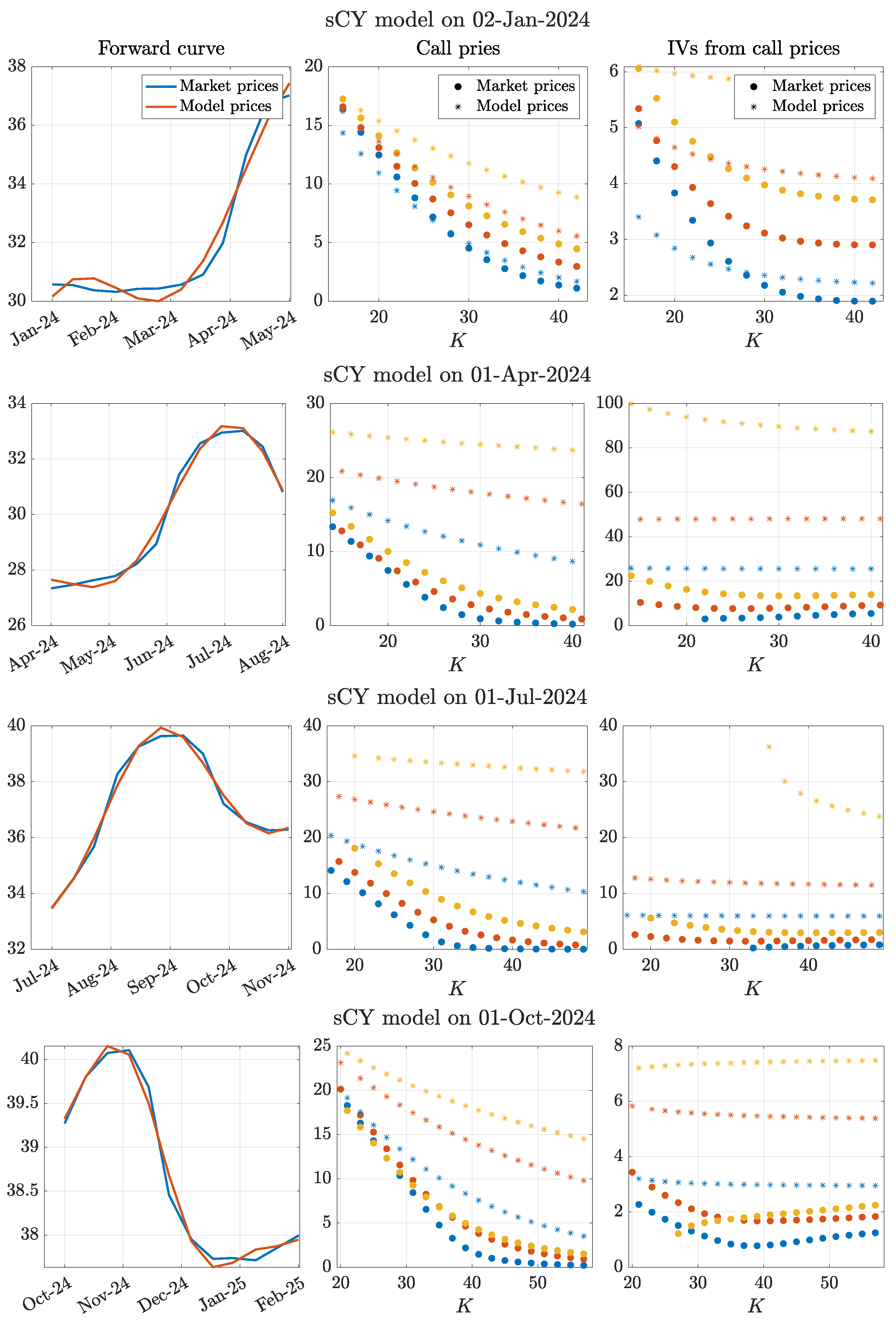
As expected, the in-sample mean squared error (IS-MSE), which corresponds to the value of the objective function of the calibration at the optimum, is extremely small, averaging 0.0578 across all the dates under analysis. Consequently, the sCY model effectively fits the forward curves. This is confirmed by the first column of panels in Figure 7, where the model-implied futures prices (in orange) closely replicate the observed market prices (in blue). A minor exception occurs on 2 January 2024, at shorter maturities, where actual futures prices remain more stable than predicted by the model. Accordingly, as shown in the first row of Table 1, the highest IS-MSE is observed precisely on that date.

It is noteworthy that the seasonal extension of the convenience yield, relative to the framework proposed by Gibson and Schwartz (1990), which was originally designed for crude oil futures and options markets that exhibit less pronounced seasonality, enables the sCY model to generate forward curves with multiple local extrema. This feature cannot be captured by a simple Ornstein–Uhlenbeck process.

While the strong in-sample fit is largely mechanical, given that the model has nine parameters while each forward curve consists of only twelve data points, the precision of the estimates appears promising for the subsequent out-of-sample evaluation on option prices.

Unfortunately, the out-of-sample performance is significantly poor. As shown in Table 1, the out-of-sample mean squared errors (OOS-MSE) are remarkably high, averaging 78.52 across all examined dates. This considerable discrepancy is clearly illustrated in the second and third columns of the panels in Figure 7, where model-implied option prices are substantially overestimated compared to observed market prices, both in absolute Euro terms and in terms of implied volatility.

The primary driver of this severe overpricing is the excessively high estimate of the spot price volatility parameter, ${\sigma }_S$. The estimated values of ${\sigma }_S$, reported in the last column of Table 1, indicate an average volatility close to 1.70, which corresponds to an unrealistically high 170% volatility9. Consequently, this inflated volatility estimate leads to a dramatic overvaluation of option prices.

This issue arises because, in the calibration of the sCY model to futures prices, ${\sigma }_S$ has only a marginal influence on the forward curve, as seen from the explicit expression of $F^{sCY}(0,T)$ in (8). Specifically, its impact is mediated through the correlation between the Brownian innovations driving the stochastic convenience yield and the spot price $\rho$ and the volatility of the convenience yield ${\sigma }_x$. As a result, ${\sigma }_S$ is difficult to estimate accurately. However, in option pricing, ${\sigma }_S$ plays a crucial role, and errors in its estimation propagate significantly, leading to the extreme mispricing observed in this calibration exercise.

4.3. Calibration of the CEV-sCY Model

We now proceed with the calibration of the CEV-sCY model. A summary of the calibration results is presented in

Table 2. In-sample mean squared error (IS-MSE), as defined in (19), out-of-sample mean squared error (OOS-MSE), as defined in (20), estimated value of ${\sigma }_S$ and of $\gamma$ obtained from the calibration of the CEV-sCY model to forward curves, following the procedure described in Section 4.1. Full calibration results are provided in Table A2 in the Appendix A.

CEV-sCY Model
Date	IS-MSE	OOS-MSE	${\mathit{\sigma }}_{\mathit{S}}$	$\mathit{\gamma }$
2 January 2024	0.1962	9.8278	0.4380	0.9475
1 Febryary 2024	0.1677	6.8720	0.4627	0.9583
1 March 2024	0.0743	1.3640	0.8853	0.9851
1 April 2024	0.0593	3.2990	0.7566	0.9686
1 May 2024	0.0600	6.4082	0.1759	0.9925
3 June 2024	0.0626	5.5388	0.3690	0.9931
1 July 2024	0.0503	6.5642	0.4150	0.9540
1 August 2024	0.0365	2.3074	0.6055	0.9559
2 September 2024	0.0063	5.9645	0.0566	0.9264
1 October 2024	0.0671	2.4783	0.5832	0.9672
1 November 2024	0.0040	4.4448	0.0719	0.9490
2 December 2024	0.0287	4.1055	0.4587	0.9578
Average	0.0678	4.9312	0.4399	0.9630

, while the full set of results is available in

Table A2. Full results from the calibration of the CEV-sCY model. IS-MSE is defined in (19) while OOS-MSE is defined in (20).

Constant Elasticity of Variance—Seasonal Convenience Yield (CEV-sCY) Model
Date	IS-MSE	OOS-MSE		${\mathit{\sigma }}_{\mathit{S}}$	${\mathit{\delta }}_{\mathbf{0}}$	$\mathit{\kappa }$	$\mathit{\theta }$	${\mathit{\sigma }}_{\mathit{x}}$	$\mathit{\rho }$	$\mathit{a}$	$\mathit{b}$	$\mathit{c}$	$\mathit{\gamma }$
2 January 2024	0.1962	9.8278		0.438	−0.6072	1.1889	0.3621	0.675	−0.3077	−0.532	6.3527	−11.2896	0.9475
1 February 2024	0.1677	6.872		0.4627	−0.3911	1.825	0.0425	1.1326	−0.1193	−0.3669	7.5744	−11.3536	0.9583
1 March 2024	0.0743	1.364		0.8853	1.0523	3.061	−0.2475	0.3852	−0.6954	−0.5465	7.8395	−11.2561	0.9851
1 April 2024	0.0593	3.299		0.7566	0.8735	2.679	−0.4734	0.3031	−0.5788	−0.6064	8.8474	−11.2539	0.9686
1 May 2024	0.06	6.4082		0.1759	−0.6184	1.5313	0.5163	0.2624	0.6123	0.5339	−8.6212	7.2576	0.9925
3 June 2024	0.0626	5.5388		0.369	−0.4829	3.5342	0.4392	0.1778	0.0171	−0.407	−8.5364	9.5515	0.9931
1 July 2024	0.0503	6.5642		0.415	−0.1587	2.5563	−0.0111	1.1658	0.0368	0.496	7.167	−11.2656	0.954
1 August 2024	0.0365	2.3074		0.6055	0.6868	3.1705	−0.1439	0.181	−0.5352	0.1954	8.6796	−11.3499	0.9559
2 September 2024	0.0063	5.9645		0.0566	0.0653	2.8266	−1.8472	0.2441	0.6279	0.7899	9.1608	−4.882	0.9264
1 October 2024	0.0671	2.4783		0.5832	−0.2814	1.4193	0.5519	1.2125	−0.0627	−0.1705	5.389	−11.324	0.9672
1 November 2024	0.004	4.4448		0.0719	1.7777	3.4618	−0.2746	0.1703	0.2053	11.4529	10.0328	1.535	0.949
2 December 2024	0.0287	4.1055		0.4587	−0.115	2.8637	0.264	1.0643	0.0309	−0.0886	8.4081	−11.1925	0.9578
Average	0.0678	4.9312		0.4399									0.963

in the Appendix A.

As expected, and in a similarly mechanical manner as observed for the sCY model, the CEV-sCY model successfully fits the observed forward curves, achieving an average in-sample mean squared error (IS-MSE) of 0.0678. Consistently, the first column of panels in Figure 8 illustrates that the forward curves generated by the model closely align with the market curves, mirroring the results obtained in Figure 7 for the sCY model. Similar to the previous calibration exercise, we note that the forward curve on 2 January 2024, remains the most challenging to replicate.

Notably, the CEV-sCY model yields an average out-of-sample mean squared error (OOS-MSE) of 4.9312, which is an order of magnitude lower than the corresponding figure obtained for the sCY model. As before, 2 January 2024 exhibits the largest deviation in option prices. This significant reduction in out-of-sample error is also evident in the second and third columns of panels in Figure 8, where model-implied option prices are now substantially closer to observed market prices, both in absolute monetary terms and in terms of implied volatility.

The improved accuracy can be attributed to a more refined estimation of the diffusive component of the spot price process S, which is now governed by both ${\sigma }_S$ and the constant elasticity of variance parameter $\gamma$. The interaction between these two parameters enables a more precise characterization of the overall variability in the spot price process, ultimately enhancing the model’s ability to predict option prices. Interestingly, the average estimate of ${\sigma }_S$ is approximately 0.44, which, when considered in isolation, is much closer to the historical volatility of the natural gas spot price process (0.52). Meanwhile, the average estimated value of $\gamma$ is 0.9630, a figure typically associated with equity markets rather than commodities. Nevertheless, the effectiveness of the local volatility component is evident, as it allows for an improved representation of the spot price process’s volatility, despite the estimated $\gamma$ being close to one, for which the two models analysed in the paper would coincide.

Remark 3. 

The two models have been calibrated monthly over a full calendar year to ensure that the results are not biased by seasonal effects. Although the OOS-MSE of the sCY model tends to be consistently above its average during the spring and summer months, possibly due to an underestimation of the volatility surrounding natural gas prices in the months ahead, there does not appear to be a clear seasonal pattern in the performance of either model. The choice between the two should therefore be guided by the intended application: for futures curve forecasting, the simpler and more computationally efficient sCY model may suffice; for option pricing or hedging purposes, the CEV-sCY model provides greater accuracy and robustness.

4.4. Hedging Performances

Accurate pricing models are essential not only for valuing derivative contracts consistently with market data but also for guiding risk management strategies such as delta hedging. In what follows, we assess the practical impact of the proposed models by comparing their performance in a delta-hedging exercise across different option moneyness levels.

Assume that at time $t=0$, one of the two proposed models is calibrated to the prevailing forward curve. Taking the perspective of the option issuer, we consider a hedging portfolio that, at time $t=0$, is short one call option written on a specific monthly futures contract maturing at time T, with strike price K, and long ${\Delta }_0$ units of the underlying futures $F(0,T)$. The value of ${\Delta }_0$ is determined according to the delta computed from the calibrated model10. Any imbalance between the short option position and the long futures position is financed through the risk-free asset.

On each subsequent day t, the model is recalibrated to incorporate the updated futures curve available at that time. The position in the underlying futures contract $F(t,T)$ is then adjusted according to the newly computed delta, ${\Delta }_t$, with the risk-free asset once again used to finance any changes in the portfolio.

At maturity T, after the option’s payoff has been settled, the hedging performance is evaluated by analysing the standard deviation of the cash flows generated by the strategy, specifically, the variability in the total cost of maintaining a delta-neutral position over the life of the option. This framework corresponds to a model-based delta hedging strategy assessed from a risk-minimization perspective. In this sense, the approach is consistent with the principles of local risk minimization commonly employed in incomplete markets.

For the numerical exercise, we set t = 0 to 1 July 2024, which, as shown in Table 1 and Table 2, lies approximately in the middle of the overall in-sample and out-of-sample performances recorded throughout the year. We consider two time horizons: one month and three months, focusing respectively on call options written on the August futures contract (with delivery at the end of July) and on the October 2024 futures contract (with delivery at the end of September). On 1 July 2024, the August futures traded at 33.485, while the October futures quoted at 35.67. Based on these values, we examine seven different strike prices for each option and assess the performance of delta-hedging portfolios with daily rebalancing.

Table 3. Summary statistics of the cash flows generated by the delta-hedging strategies described in Section 4.4. For the standard deviations, values in bold indicate the lower (i.e., better) result between the two models.

Time to maturity = 1 month; at-the-money level = 33.485
K	27		30		33		37		40
	sCY	CEV-sCY	sCY	CEV-sCY	sCY	CEV-sCY	sCY	CEV-sCY	sCY	CEV-sCY
Sum	−0.0362	0.1556	0.0470	0.1546	0.7514	0.9849	0.2476	0.0998	−0.0719	−0.2251
Average	−0.0018	0.0078	0.0023	0.0077	0.0376	0.0492	0.0124	0.0050	−0.0036	−0.0113
Std. Dev.	0.1352	0.0843	0.1786	0.1568	0.1425	0.1135	0.1573	0.1320	0.1264	0.1077
Time to maturity = 3 months; at-the-money level = 35.76
K	29		32		36		39		43
	sCY	CEV-sCY	sCY	CEV-sCY	sCY	CEV-sCY	sCY	CEV-sCY	sCY	CEV-sCY
Sum	0.7845	0.6137	1.9750	1.223	4.2070	4.0094	4.2118	5.3115	2.8450	2.9188
Average	0.0125	0.0110	0.0324	0.0218	0.0695	0.0678	0.0701	0.086	0.0484	0.0462
Std. Dev.	0.0900	0.0722	0.0942	0.1612	0.2577	0.3745	0.2658	0.2598	0.2477	0.1641

summarizes the results of the hedging analysis. As observed, aside from the at-the-money options, where both models yield comparable outcomes without a clear advantage, the CEV-sCY model consistently demonstrates superior performance as the strike moves either in- or out-of-the-money. In these cases, it exhibits lower variability in the cash flows generated by the hedging strategy. This finding highlights the importance of the local volatility component in better capturing the behavior of options that are far from the money. Consequently, as pointed out in Remark 3, the CEV-sCY model appears more suitable for market participants interested in natural gas options, as opposed to those focused solely on futures trading, for whom the sCY model alone remains reasonably effective.

5. Conclusions

This paper examines the pricing of natural gas futures and options through a unified spot price modeling framework. Building upon the seminal work of Gibson and Schwartz (1990), we extend the classical two-factor model by incorporating a deterministic seasonal component in the stochastic convenience yield to capture the strong seasonality observed in the natural gas futures market. While this extension successfully fits futures prices, it fails to accurately reproduce observed option prices, suggesting that a more flexible volatility structure is required.

To address this limitation, we introduce a further refinement by incorporating a local volatility factor in the spirit of the Constant Elasticity of Variance (CEV) model by Cox (1975). This enhancement allows for a more accurate representation of the underlying spot price dynamics, leading to a significant improvement in option pricing performance. Since closed-form solutions for futures and options prices are no longer available in this extended setting, we propose an efficient lattice-based numerical approach for pricing derivatives.

Our findings highlight the importance of both seasonality and local volatility in modeling natural gas markets. By bridging the gap between futures and options pricing models, this study contributes to the existing literature on commodity derivatives and offers a framework that better captures the empirical behavior of market prices.

Future research could explore the incorporation of fully stochastic seasonal and volatility components, as well as extensions that account for jumps or regime-switching dynamics in the spot price process.