Article

Time Restrictions on Life Annuity Benefits: Portfolio Risk Profiles

by
Annamaria Olivieri
1,* and
Ermanno Pitacco
2
1
Department of Economics and Management, University of Parma, Via J.F. Kennedy 6, 43125 Parma, Italy
2
MIB Trieste School of Management, Largo Caduti di Nassiriya 1, 34142 Trieste, Italy
*
Author to whom correspondence should be addressed.
Risks 2022, 10(8), 164; https://doi.org/10.3390/risks10080164
Submission received: 5 June 2022 / Revised: 6 August 2022 / Accepted: 9 August 2022 / Published: 12 August 2022
(This article belongs to the Special Issue Longevity Risk Modelling and Management)

Abstract

:
Due to the increasing interest in several markets in life annuity products with a guaranteed periodic benefit, the back-side effects of some features that may prove to be critical either for the provider or the customer should be better understood. In this research, we focus on the time frames defined by the policy conditions of life annuities. While the payment phase coincides with the post-retirement period in the traditional annuity product, arrangements with alternative time frames are being offered in the market. Time restrictions, in particular, could be welcomed both by customers and providers, as they result in a reduction in expected costs and equivalence premiums. However, due to the different impact of longevity risk on different age ranges, time restrictions could increase risks to the provider, at least in relative terms. On the other hand, time restrictions reduce the duration of the provider’s liability, which should therefore be less exposed to financial risk. We focus on this issue, examining the probability distribution of the total portfolio payout resulting from alternative time frames for life annuity arrangements, first addressing longevity risk only, and then including also financial risk. The discussion is developed in view of understanding whether a reduction in the equivalence premium implied by time restrictions should be matched by higher premium loading and required capital rates.

1. Introduction

The progressive shift in many countries from defined benefit to defined contribution pension plans has recently increased the interest in life annuity products with a guaranteed periodic benefit. Nevertheless, some disadvantages of (standard) life annuities make the product not very attractive, as it is evidenced by the fact that annuity markets are still undersized. Some features should be improved by moving from the basic product (the single premium immediate life annuity (SPIA) with lifelong benefit payment) to more structured products, for example by adding riders (that is, supplementary benefits), adopting restrictions on the age intervals covered, or allowing for individual risk factors (so as to quote annuity rates, at least to some extent, “tailored” to specific customer’s features).
In this research, we focus on restrictions on the age intervals covered by annuity benefits. The traditional design for life annuities assumes that the payment phase coincides with the post-retirement period. Alternative time frames have been offered by providers, or just designed in the literature, in an attempt to encourage the demand. Indeed, time restrictions reduce the expected value of payments, and then the equivalence premium; this way, the annuity is perceived to be less expensive. However, the longevity risk to which an annuity provider is exposed has different impacts on different age ranges, with greater incidence at old ages. When time restrictions are introduced by delaying the payments to higher ages, we cannot take for granted that the reduction in the expected value of the provider’s payout is matched by a proportional reduction of its dispersion. Thus, we cannot exclude the idea that a reduction in the equivalence premium should be complemented by an increase in the premium loading rate, due to a higher dispersion (at least in relative terms) of the provider’s liabilities. This issue has received little attention in the literature, whereas we think it should be more carefully examined, so as to achieve a clearer understanding of the various side effects of alternative policy conditions. In this paper, we develop an analysis in this respect, by assessing the probability distribution of the total provider’s payout for a number of life annuity arrangements (ranging from the immediate whole life annuity to the deferred term life annuity). We focus on some specific policy time frames or payment time frames, especially looking at time restrictions on benefit payment, and compare the corresponding portfolio risk profiles, in particular in terms of the right tail of the probability distribution of the present value of future payments. We find that, per unit of expected value, annuity arrangements which restrict payments to the oldest ages may show a heavier right tail, thus suggesting the need for higher premium loadings or larger capital amounts under such policy conditions.
A stochastic mortality assumption is adopted, allowing us to include both components of longevity risk in the analysis, that is, the idiosyncratic risk (due to mortality random fluctuations) and the aggregate risk (due to uncertainty in future mortality trend). The value of the provider’s liability is also exposed to risks other than longevity, in particular financial risks, that require careful attention. In a first step of the investigation, with respect to risks other than longevity, we adopt a deterministic setting. This choice is justified by the fact that when comparing alternative annuity designs, a significant role should be played by the different age ranges involved, and (unlike other risks) only longevity risk is age-related. However, time restrictions reduce the duration of the provider’s liability, reducing exposure to financial risk. In a second step of the investigation, we therefore also include financial risk. We find a trade-off between the opposite effects produced by time restrictions on the overall exposure to longevity and financial risk, depending on the scenario (in particular, depending on the lower or higher uncertainty about the mortality dynamics and the lower or higher volatility of investments).
The remainder of the paper is organized as follows. In Section 2, a literature review is provided, including textbooks and reports describing general features of life annuity products and papers specifically dealing with alternative annuity structures, with a particular focus on those introducing time restrictions, i.e., old-age life annuities on the one hand, and annuity arrangements involving term life annuities on the other.
The three following sections constitute the core of the paper. In particular, Section 3 focusses on various annuity structures, with special emphasis on possible restrictions on the annuity payout phase. The valuation framework adopted in assessing the portfolio risk profile is described in Section 4. The impact of diverse annuity structures on results of interest is assessed in Section 5, where numerical examples are presented and discussed.
Final remarks in Section 6 conclude the paper.

2. Literature Review

Actuarial models for life contingency products and life annuities in particular are dealt with by all actuarial textbooks, in which premium and mathematical reserve calculations are addressed. See, for example: Bowers et al. (1997), Dickson et al. (2020), Gerber (1995), and Olivieri and Pitacco (2015).
A compact and effective presentation of annuities, and life annuities in particular, is provided by Macdonald (2004). The book by Pitacco (2021) is specifically devoted to life annuity products and their relevant actuarial features, with a special focus on innovations in product design.
Restrictions on the payout phase as a way to reduce the expected number of payments and then the premium amount, directed towards more attractive products, are discussed by Milevsky (2005), who designs the advanced life delayed annuity (ALDA) product, otherwise known as old-age life annuity or longevity insurance or annuity with a deductible. Gong and Webb (2010) investigate the money’s worth to the individual of an ALDA, in particular in comparison to alternative post-retirement solutions, and discuss optimal annuitization strategies including old-age annuities. The money’s worth of an old-age annuity is also analysed by Stephenson (1978). The structure of longevity insurance has been generalized by Huang et al. (2009), suggesting the design of the ruin contingent life annuity (RCLA).
Restrictions on the payout phase can be introduced by way of an upper limit to the number of payments, instead of a deductible. This is embedded in the design of term life annuities, that is, annuities which pay the benefit while the individual is alive, for at most a given number of years. While a stand-alone term life annuity does not provide an adequate longevity protection to the individual, as it leaves the individual exposed to longevity risk at the ages when it is most severe, a term life annuity can constitute a component of an annuity structure called “extendable annuity”. Such a design is discussed, for example, by Rocha et al. (2011). After the last payment of the term life annuity, the benefit payment can be extended over time. At each renewal, the provider can update the assumptions used to assess the annuity rate, while the individual can gradually decide, instead of only once at issue, the amount of wealth to be used to purchase the annuity. Clearly, an extendable annuity can be arranged with a sequence of term life annuities, eventually followed by lifetime payments. Exploring the optimal arrangement of an extendable annuity falls outside the scope of this paper; however, term annuities are considered in comparative terms with alternative choices of the payment time frames.
While the old-age life annuity constitutes a modern form of deferred life annuity, where the payout phase is postponed after retirement, the traditional design of a deferred life annuity includes a payout phase starting at retirement, preceded by a savings process during the working period. The critical issue in this case is given by the time at which the annuity rate is stated. The sooner the annuity rate is stated, the stronger the guarantee and the higher the risk borne by the annuity provider. In this context, we find the guarantee annuity option (GAO) product. The impact of the GAO is, in particular, analyzed by Boyle and Hardy (2003). While we consider deferred life annuities in comparative terms with alternative time frames in the paper, the issue about when it is better to set the annuity rate is not addressed.
As we have already noted, most of the contributions to the existing literature discuss innovations in the definition of annuity time frames as a way to improve the attractiveness of the products, thanks to the reduction in the premium amount arising because of the lower expected number of payments. However, annuity premiums also include loadings, whose size should be consistent with risk arguments. To the best of our knowledge, this issue has not been discussed in depth in the literature.
Assessing the risk profile of a life annuity portfolio calls for a stochastic model, allowing for the main risk causes and components, in particular financial and longevity risk and the related components. As far as longevity risk is concerned, models allowing for both the components, i.e., both the idiosyncratic risk (that is, the risk of random fluctuations in mortality) and the aggregate risk (that is, the risk of systematic deviations), should be considered. The demographic and actuarial literature offers a number of modelling possibilities. After the seminal paper by Lee and Carter (1992), several stochastic mortality models have been discussed in the literature, either extending the Lee–Carter model or resembling its main structure (just considering the earlier contributions, we mention Brouhns et al. (2002), Renshaw and Haberman (2003, 2006), and Cairns et al. (2006)), or exploring alternative approaches. We mention, in particular, the application of affine stochastic models, first examined by Biffis (2005) and Schrager (2006), and further carried out by many other authors, including Blackburn and Sherris (2013). The literature also includes many reviews of various alternative models. Among the most recent and updated, we mention Hunt and Blake (2021). In the present paper, we adopt the stochastic mortality model proposed and implemented in Olivieri and Pitacco (2009), for the reasons explained in Section 4.2. Regarding financial risk, we adopt a classical log-normal model for the investment return; despite its simplifications, the log-normal model is commonly implemented in insurance applications, in particular when multiple risk sources are considered. Among the recent contributions, see for example Hieber et al. (2019), Orozco-Garcia and Schmeiser (2019), Bacinello et al. (2021), and Ghalehjooghi and Pelsser (2021).

3. Time Frames for the Policy and the Benefit Payment

3.1. Traditional Alternative Post-Retirement Income Solutions

In the context of personal wealth management, several post-retirement income solutions are usually considered. According to a simplified approach, the basic alternatives are the following ones (see, for example, Pitacco (2021)):
  • the immediate whole life annuity, purchased at the retirement time against a single premium (that is, the SPIA);
  • the deferred life annuity, purchased during the working period, usually financed by a sequence of premiums (which constitute the so called “accumulation annuity”), with benefit payment commencing at the retirement time;
  • the income drawdown, that is, a sequence of withdrawals from a fund, starting at the retirement time.
More solutions can be conceived and implemented by changing the “standard” time frames implied by the above alternatives.

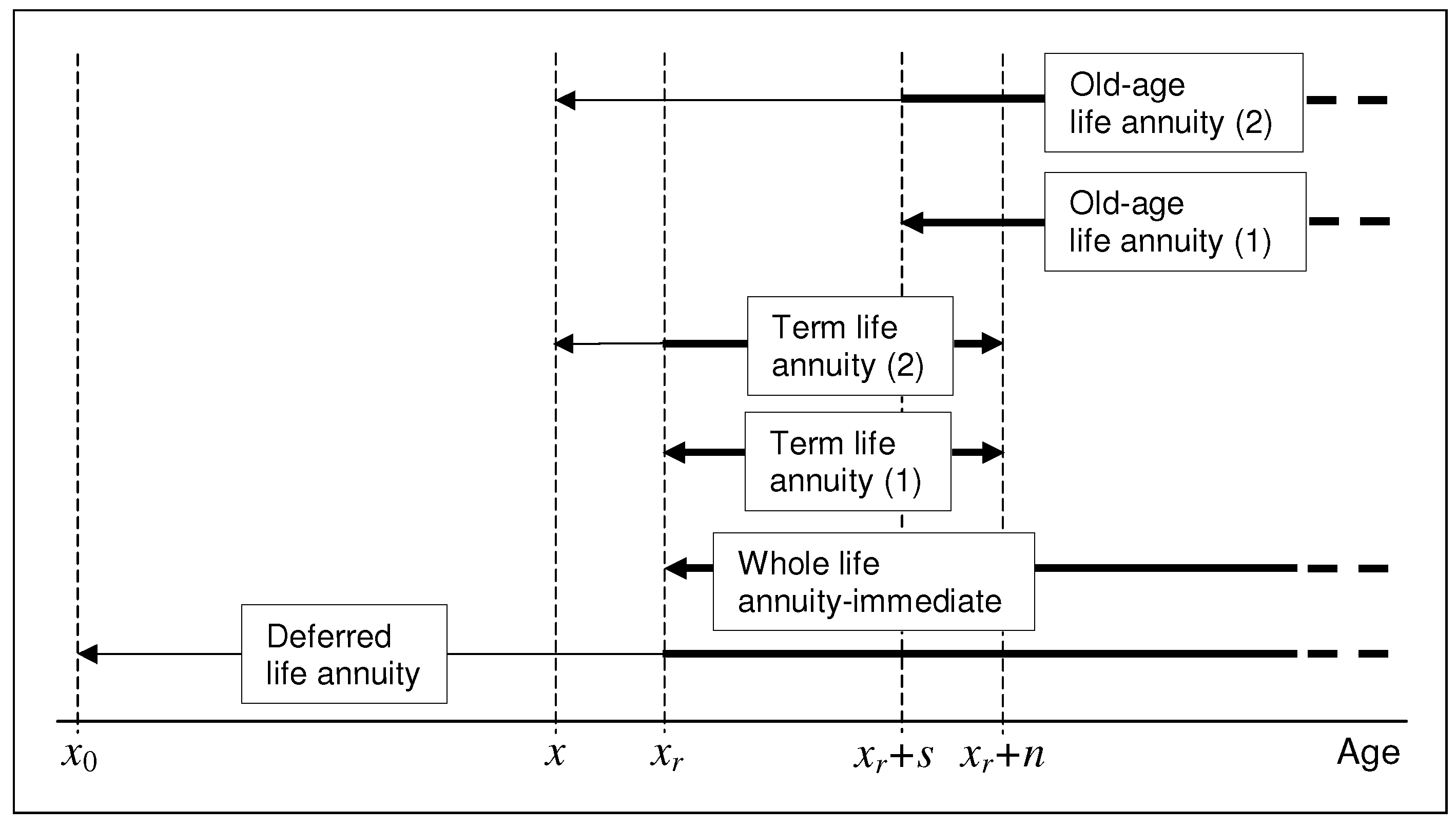
3.2. A Reference Scheme including Additional Alternatives

In what follows, we refer to life annuities with a flat benefit profile (in nominal terms). Thus, no indexing mechanism or profit participation scheme is considered. Benefits are assumed to be paid on an annual basis.
To define a set of life annuity arrangements, we adopt the following notation:
  • x 0 = an age within the working period (e.g., at the beginning of the accumulation period);
  • x r = the age at retirement;
  • x = an age before retirement time ( x 0 x x r ; e.g., the age at which the annuity rate is stated);
  • n = the number of years of term annuity payments;
  • s = the length in years of the delay period (e.g., in old-age life annuities).
A set of annuity arrangements is shown in Figure 1. Each line represents the time frame covered by the policy. In particular, each thick line represents the benefit payment time frame.

3.2.1. Deferred Life Annuities

In a deferred life annuity, the policy time frame starts at an “initial” age x 0 , that is, the beginning of the accumulation phase, so that the deferral period coincides with the accumulation period. According to the traditional actuarial terminology, the deferred life annuity is frequently meant as a contract in which all the policy conditions (the annuity rate included) are stated at the time of policy issue. More generally, the policy conditions can be stated at a time following the policy issue, and, of course, at the latest, at the end of the accumulation phase. Whatever is the time when policy conditions are stated, a lifelong benefit is paid.

3.2.2. Immediate Whole Life Annuity

According to this arrangement, the policy time frame coincides with the payout phase. Policy conditions are stated at the policy issue, which is also the time when the relation between the single premium and the annuity benefit is defined. A lifelong benefit is paid.

3.2.3. Term Life Annuities

A term life annuity pays the benefit at most for a given number n of years, provided that the annuitant is alive. A deferral period can either be included (see term life annuity (2) in Figure 1) or not (see term life annuity (1)). In case of the deferral period, policy conditions can be stated at the beginning of the period itself or later (see Section 3.2.1).

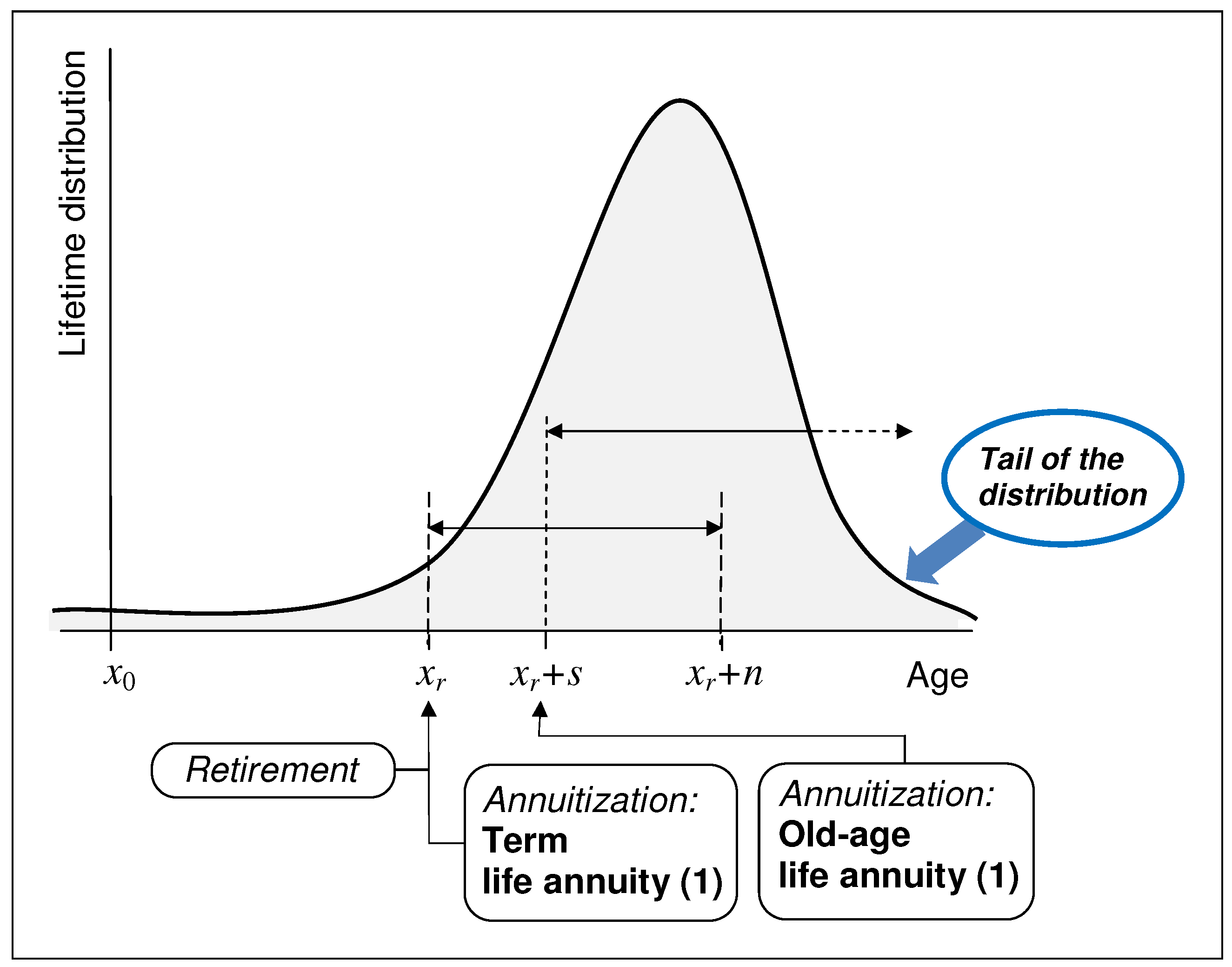
3.2.4. Old-Age Life Annuities

In old-age life annuities, the time frame reduction involves shifting the payment commencement to an age higher than the retirement age x r . While this arrangement leaves the initial part of the post-retirement period uncovered, it provides the retiree with “ultimate” protection against longevity risk, since it covers the tail of the lifetime distribution.
The post-retirement income can be obtained, throughout the s-year delay period, via a temporary income drawdown. As no mutuality mechanism is involved, this arrangement is compatible with a bequest motive (albeit limited to the delay period).
As in the case of term life annuities, a deferral period can either be included (see old-age life annuity (2) in Figure 1) or not (old-age life annuity (1)). In case of the deferral period, policy conditions can be stated at the beginning of the period itself or later.

3.3. Longevity Risk Transfers

As is well-known, by underwriting a life annuity, individuals transfer their longevity risk, i.e., the risk of outliving their assets, to a provider. A significant diversity in the amount of the individuals’ longevity risk transferred from the annuitant to the annuity provider features the various life annuity arrangements described in Section 3.2.
In a whole life and in a deferred life annuity, individuals’ longevity risk in the post-retirement period is totally transferred to the annuity provider. Further, a larger amount of individuals’ longevity risk is transferred in a deferred life annuity provided that the annuity rate is stated before the payment commencement.
Restrictions on the time frame of benefit payment conversely reduce the individuals’ longevity risk transfer. In particular, term life and old-age life annuities lead to “opposite” reductions in risk transfer. Uncovered age intervals are ( x r + n , + ) in a term life annuity and ( x r , x r + s ) in an old-age life annuity, respectively (see Figure 2).
It is also well known that, from the point of view of the provider, the longevity risk shows two components: the idiosyncratic longevity risk, due to the diversity between the lifetime of each individual and the expected lifetime, and the aggregate longevity risk, due to the possible difference between the expected lifetime and the average lifetime of all annuitants. Annuity designs implying different transfers of individuals’ longevity risk impact differently on the longevity risk to which the provider is exposed. Intuitively, time restrictions reduce the total size of longevity risk to the provider. However, in relative terms, the risk taken by the provider could be higher, in particular when payments are limited to the right tail of the individuals’ lifetime distribution. In view of defining appropriate risk management solutions, an investigation of the provider’s portfolio risk profile is recommended; this is what we perform in Section 5. Of the various risk management actions, we focus on capital required and premium loading.

4. Valuation Framework

4.1. Present Value of Future Benefits

In what follows, we consider a discrete-time fixed-amount annuity in arrears, i.e., with payments at the end of each year. To simplify notation, flat payments are assumed, with b denoting the annual benefit amount. Our main aim is to compare alternative annuity designs, in terms of the different level of risk retained by the provider.
Conventionally, we set time 0 at age x 0 . Let T denote the benefit payment time frame; with reference to the cases discussed in Section 3.2 (see also Figure 1), we have: T = ( r , ) for an immediate whole life annuity purchased at retirement time, as well as for a deferred life annuity purchased during the working period; T = ( r , r + n ] for a term life annuity (purchased prior to or at retirement); and T = ( r + s , ) for an old-age life annuity (either with a deferral period or not).
Let τ denote the time when the annuity is issued: 0 τ < r for a deferred life annuity (either whole life or temporary); τ = r for an immediate whole or term life annuity; and τ = s for an old-age life annuity.
We define the discount factor over the time interval ( t + τ , k ) as v ( t + τ , k ) = e R ( t + τ , k ) , where R ( t + τ , k ) is the log return on investments over the same time interval. In the numerical implementation, in a first step of the analysis, we assume a deterministic return, so as to more clearly understand the effect of time restrictions on longevity risk; then, in the second step of the analysis, we take a more comprehensive perspective and assume a stochastic return.
We focus on a cohort consisting of n x τ identical annuities issued at time τ ; annuities are identical because of annuitants’ age, x τ = x 0 + τ , benefit amount, and annuitants’ mortality profile. After t years since issue, t 0 , the number of surviving annuitants is N x τ + t , and is random. For each annuity issued at time τ , we assess the present value of future benefits at time t, t 0 , as follows:
PVFB t = k T ( τ + t , ) b · v ( t + τ , k ) · N x τ + k n x τ ,
which is a random quantity, because of N x τ + k and the return R ( t + τ , k ) (when stochastic). The random variables N x τ + k and R ( t + τ , k ) are assumed to be independent.
In order to obtain the usual summary statistics for PVFB t , the ratio N x τ + k n x τ , i.e., the proportion of survivors at age x τ + k out of the initial n x τ , and the return R ( t + τ , k ) must be modelled. Regarding the number of survivors, if we assume a deterministic financial return and simply replace N x τ + k n x τ with a given (for example, best-estimate) survival probability, then we (only) obtain the traditional actuarial value of future benefits. Conversely, if N x τ + k n x τ is kept random, then dispersion measures for PVFB t , accounting explicitly for longevity risk, can be assessed. If mortality rates are assumed to be deterministic, only random fluctuations may affect such dispersion measures. In order to also account for aggregate longevity risk, mortality rates must be assumed to be stochastic. This is the approach we follow, adopting the model described in Section 4.2. Regarding the financial return, as already mentioned, we alternatively assume a fixed and a random return. The former choice allows us to single out the impact on the present value of future benefits of longevity risk only, whereas the latter choice provides a more comprehensive overview of the risk profile of the provider’s liability. The financial model is described in Section 4.3.
We point out that we do not aim to perform a fair valuation in a market-consistent style. We rather examine the realistic probability distribution of the present value of future benefits and comment on the magnitude of the loading and required capital that are suggested by its tail. We assess the best-estimate value of PVFB t , that we denote as PVFB t BE , based on best-estimate survival probabilities and financial return defined at time τ . Further, we assess the ε quantiles of PVFB t , that we denote as PVFB t ε , for convenient values of ε . The difference PVFB t ε PVFB t BE can be interpreted as an additional amount required on top of the best-estimate value of future benefits because of the risks to which the provider is exposed.
At issue time τ , we assume that each individual contributes the amount S. Given an accepted probability of loss 1 ε and for a chosen annual amount b, we consider the following pricing principle:
S = PVFB 0 ε .
With reference to the best-estimate value, (2) implies a premium loading rate equal to PVFB 0 ε PVFB 0 BE 1 .
In line with the Solvency II philosophy, we assume that, at any time t, the provider needs to hold a total amount of funds so as to avoid default with 99.5% probability. While the possible default is notionally detected over a year, the standard formula adopted for longevity risk actually refers to the whole life of the cohort (indeed, the Solvency II standard formula deterministically identifies the required capital for longevity risk as the increase in the net asset amount over a year because of a 20% reduction in mortality rates at all ages; therefore, in practice, the possible loss suffered by the provider must be measured over the remaining life of the cohort, as discussed in Blackburn et al. (2017)).
In our setting, the amount of funds required to avoid default throughout the cohort’s life with a 99.5% probability can be identified with PVFB t 0.995 , on a policy basis. The assessment of PVFB 0 0.995 (i.e., for t = 0 ) allows us to identify the additional capital required at issue, on top of the initial amount S. Indeed, if PVFB 0 0.995 is the total amount of resources required at issue, then PVFB 0 0.995 S = PVFB 0 0.995 PVFB 0 ε is the required capital. The assessment of PVFB t 0.995 for times t > 0 , i.e., after issue, allows us to project the time profile of the capital resources that will be required throughout the whole cohort’s life; these resources will be partially covered by the remaining share of S and by capital. Assessing the remaining share of S throughout the cohort’s life is not addressed in this paper (we only discuss the total amount of resources required).

4.2. Mortality Model

We represent mortality with the model described in Olivieri and Pitacco (2009), that we summarize briefly in this section.
We refer to the cohort of n x τ annuities issued at time τ . We assume that a best-estimate assumption is available for the mortality rates, that we denote as q x τ + t ( τ ) . However, the mortality rate at age x τ + t is random; we use the notation q ˜ x τ + t .
Here, we just recall the features of the model useful for understanding the assessment of the ε quantiles of PVFB t in Section 5, while we refer to Olivieri and Pitacco (2009) for a detailed description of the model.
We assume:
q ˜ x τ + t = q x τ + t ( τ ) · Z x τ + t ,
where Z x τ + t is a (positive) random coefficient (ensuring 0 q ˜ x τ + t 1 ), expressing a deviation of the mortality rate in respect of the best-estimate value available at time τ . Such a coefficient is suitable to represent aggregate deviations in mortality. We assume:
Z x τ + t Gamma ( α x τ + t , β x τ + t ) ;
then, q ˜ x τ + t also follows a Gamma distribution, with parameters obtained from those of the probability distribution of Z x τ + t . Conditional on a given value of Z x τ + t (i.e., conditional on a given mortality rate), the individuals’ lifetimes are independent and the number of deaths reported by the cohort can be modelled with a Poisson distribution. Having assumed a random mortality rate, whose probability distribution follows a Gamma law, we obtain that the unconditional distribution of the annual number of deaths is described by aNegative Binomial (or Poisson–Gamma) law. We point out that the Poisson distribution measures the random fluctuations in the mortality of the cohort, whereas (as mentioned above) aggregate deviations are measured by the probability distribution of Z x τ + t (Gamma, in our case).
At time τ , there is little information about the future mortality dynamics of the cohort. However, in the following years, additional information is carried by the observed numbers of deaths. We include such information in the probability distribution of Z x τ + t , and then of q ˜ x τ + t , as follows. At time τ , we set α x τ + t = α ¯ τ and β x τ + t = β ¯ τ , with α ¯ τ and β ¯ τ based on initial information. Then, year after year, such parameters are updated, via an inferential procedure based on the information provided by the observed numbers of deaths. In particular, after h years of observation, once the numbers of deaths d x τ , d x τ + 1 , , d x τ + h 1 and the numbers of survivors n x τ , n x τ + 1 = n x τ d x τ , , n x τ + h = n x τ + h 1 d x τ + h 1 have been reported, the initial values α ¯ τ and β ¯ τ are replaced, respectively, with the following values: α ¯ τ + h = α ¯ τ + k = 0 h 1 d x τ + k , β ¯ τ + h = β ¯ τ + k = 0 h 1 n x τ + k · q x τ + h 1 ( τ ) . This update of the parameters α x τ + t , β x τ + t introduces an implicit correlation among the coefficient’s Z x τ + t , which is something one expects when thinking of the underlying long-term trend of mortality. Nevertheless, fluctuations in the number of deaths in the opposite direction are still possible at any time.
The description above should allow the key features of the model to be grasped. While preserving computational tractability, parameters are quickly updated to the emerging experience. This way, at any point in time, trend effects are quite naturally embedded in the simulation of the future number of survivors. On the other hand, if initial parameters are biased, either because of the lack of data or changes in the mortality dynamics not detectable from past experience, the updating process ensures a consistent adjustment of the future forecasts. The model is particularly advantageous when a best-estimate life table is made available by an independent institution, as is the case in many markets; for commercial reasons, the provider could find it appropriate (or necessary) to make use of such a table, in particular for pricing. However, by its nature, a best-estimate life table only provides deterministic mortality rates. In case the provider has no direct access to the data-set or the technology by which the best-estimate life table is processed, the model described in this section still allows it to perform stochastic valuations of the provider’s liabilities, also accounting for aggregate longevity risk. If a market best-estimate life table is not available, the provider can resort to an external source (such as a best-estimate life table recommended for similar populations), or to a best-estimate life table produced internally. As already noted, any bias in the initial set of parameters should be adjusted gradually in time, thanks to the updating process. In this regard, we note that the model allows us to produce new best-estimate life tables at any time, updating the initial one on the basis of the experience gained so far.
Regarding the choice of the mortality model, we finally note that our aim in this paper is not to identify the most appropriate premium loading or size of the capital required for any specific annuity designs. Rather, we aim to develop a comparative analysis of alternative designs. In this respect, rather than the specific model, what matters is taking into account the longevity risk, in both its components.

4.3. Financial Model

As already noted, with regard to financial risk we adopt, alternatively, a deterministic and a stochastic approach, the former allowing us to single out the impact of longevity risk on the different annuity designs.
In the deterministic setting, a flat annual interest rate is assumed for simplicity. A term-structure of interest rates could be used instead, but this would not change what we can learn from the assessments performed with a flat rate.
In the stochastic setting, we assume that the log return R ( t + τ , k ) is Normally distributed, with mean μ · ( k ( t + τ ) ) and standard deviation σ · ( k ( t + τ ) ) . We consider μ as representing the best-estimate assumption for the financial (instantaneous) log return.
Similarly to what was noted for the mortality model, also regarding the financial model, we point out that the model choice certainly affects the numerical results, in particular in terms of their absolute values. More proactive or structured investment strategies that justify alternatives to the log-normal assumption could result in lower losses, as well as in higher profits to the provider. However, we stress that in this paper we are primarily concerned with the impact of longevity risk, by itself and in interaction with other major risks.

5. Portfolio Risk Profiles: Numerical Results

5.1. Arrangements

Table 1 lists the types of annuities we consider in the numerical implementation, specifying the entry age, possible deferment, and the maximum duration of the annuity payments. The labels of the arrangements are shown in Figure 1. Considering common situations in the market, where a usual retirement age is 65, and people are encouraged to plan their post-retirement income at least 10–15 years in advance, the standard retirement age is assumed to be x r = 65 , while time 0 is set 15 years before; thus, x 0 = 50 . All annuities are issued in the current calendar year (i.e., 2022). This means that, depending on the age at entry, the various annuities could be addressed to individuals born in different calendar years, as reported in Table 1. More specifically, the immediate whole life annuity, the term life annuity (1), and the old-age life annuity (2) are underwritten by individuals born in 1957; the deferred life annuity and the term life annuity (2) are underwritten by individuals born in 1972; the old-age life annuity (1) is underwritten by individuals born in 1942. The year of birth matters in the choice of the parameters of the mortality model, as different cohorts usually show different mortality dynamics.

5.2. Parameters

Best-estimate mortality rates are taken from the latest Italian projected life table, the so-called life table A62; see ANIA (2014). The life table is cohort-based; it has been constructed by the National Association of Italian Insurers (ANIA), starting from projections processed by the Italian Statistical Institute (ISTAT) for the Italian population. The ANIA has reworked the ISTAT projections by applying some adjustments in consideration of the self-selection effects typical of annuity portfolios, and by adopting an age-shifting rule to obtain cohort-specific life tables starting from the life table for a reference cohort. Indeed, “A” stands for annuitants, while “62” is the reference cohort (people born in 1962). We prefer to make use of a best-estimate life table available in this format, rather than working out a best-estimate life table based on an analytical model, because we take the perspective of a provider who considers it to be appropriate (or necessary), for commercial reasons, to perform baseline assessments by using the standard market best-estimate life table. Alternative choices of the best-estimate table may not alter the results, at least in comparative terms (we also note that if we had considered a different issue calendar year, different cohorts would be involved and, as a result, slightly different best-estimate tables would be used. In this respect too, there would be no significant difference in the numerical results). For the numerical implementation in this paper, from the life table A62, we extract mortality rates for males, and we disregard self-selection adjustments.
As far as deviations from best-estimate mortality rates are concerned, at the time of issue, for all cohorts we set α ¯ τ = β ¯ τ , so that E τ [ Z x τ + t ] = 1 , E τ [ q ˜ x τ + t ] = q x τ + t ( τ ) (the subscript of the symbol E makes the time at which the expected value is assessed explicit, thus meaning that the state of information about mortality is specified at that time). Based on the information carried by the observed numbers of deaths up to time h after issue, we then have E τ + h [ Z x τ + t ] = α ¯ τ + h β τ + h ¯ and E τ + h [ q ˜ x τ + h ] = α ¯ τ + h β τ + h ¯ · q x τ + t ( τ ) , where α ¯ τ + h β τ + h ¯ 1 , depending on the realized numbers of deaths in respect of their prior expected values. The numbers of deaths is simulated for each cohort, independently from those obtained for the other cohorts.
Data for estimating the initial parameters of the Gamma distribution are scarce, as these parameters capture how likely is to experience alternative long-term trends compared to the best-estimate one. We then take a sort of “what if” approach in this respect, by considering two alternative assumptions. We alternatively choose α ¯ τ = β ¯ τ = 100 and α ¯ τ = β ¯ τ = 1000 . With α ¯ τ = β ¯ τ = 100 , the coefficient of variation of Z x τ + t based on the information available at time τ takes value 0.1; with α ¯ τ = β ¯ τ = 1000 , it takes value 0.0316. This means that we should expect larger aggregate deviations from the best-estimate life table with α ¯ τ = β ¯ τ = 100 , than with α ¯ τ = β ¯ τ = 1000 . This is why we will refer to the choice α ¯ τ = β ¯ τ = 100 as a scenario with major aggregate deviations in mortality, whereas the choice α ¯ τ = β ¯ τ = 1000 will be referred to as a scenario with moderate aggregate deviations in mortality (we stress, however, that “moderate” and “major” are only used in comparative terms between the two assumptions).
As far as the benefit amounts are concerned, we set b = 1 monetary unit. For each arrangement, the initial amount S contributed by each individual is obtained via Equation (2), which is assessed alternatively by setting ε = 0.95 or ε = 0.99 . We point out that the quantiles PVFB 0 ε , as well as the quantiles PVFB t 0.995 , t = 0 , 1 , , are obtained through stochastic simulation.
When considering a fixed investment return, the comparisons of the quantiles of PVFB t are only marginally affected by the return level (unless the return is so high that it flattens all the values, which is not currently a realistic situation). Thus, to simplify the interpretation of the results, we set a 0% annual return; this way, PVFB t expresses the (random) duration of the annuity.
As far as the parameters of the stochastic financial return are concerned, the most appropriate choice clearly depends on the asset composition. To this regard, we note that fixed-benefit annuities, due to their embedded guarantees, should be backed by conservative investment strategies. So, in principle, it is reasonable to refer to assets with a low volatility. We test two alternative risk–return asset profiles: one with lower and one with higher volatility and mean return; more precisely, we assume alternatively μ = ln ( 1.02 ) , σ = 0.005 and μ = ln ( 1.03 ) , σ = 0.01 . In comparative terms, we refer to the two assumptions, respectively, as lower and higher investment volatility.

5.3. Results and Discussion: Longevity Risk Only

In this section, in order to single out the role of longevity risk, a deterministic financial setting is implemented, with a 0% investment return. The investigation is then more comprehensively performed in the next Section 5.4, where we jointly consider longevity and financial risk.
Table 2 quotes the best-estimate present value of future benefits at issue. As just noted (at the end of Section 5.2), having set a 0% interest rate, PVFB 0 expresses the random total number of payments, of which PVFB 0 BE is the expected value (in the best-estimate scenario), at issue. The magnitude of such a number is explained by the benefit payment age frames, that we include in Table 2 to facilitate interpretation. We point out that 121 is the maximum attainable age in the life table A62. When comparing the best-estimate present value of future benefits of an immediate annuity with that of a deferred annuity providing payments in the same age frame (i.e., whole life vs. deferred life annuity, term life annuity (1) vs. (2), old-age life annuity (1) vs. (2)), and the different values taken by PVFB 0 BE are due to two opposite effects. On the one hand, the deferment reduces the probability of the future payments. On the other hand, different best-estimate life tables are available for different cohorts, predicting lower mortality (on average) for younger cohorts. Depending on the trade-off between these two opposing effects, the best-estimate present value of future benefits at issue is lower for the deferred annuities (as is the case of the term life annuity (2) vs. (1) or the old-age life annuity (2) vs. (1)), or higher (as is the case of the deferred life annuity vs. the immediate whole life annuity).
With reference to the time of issue, Table 3 quotes the ε quantiles of the present value of future benefits (expressed as a % of the best-estimate value, i.e., PVFB 0 ε PVFB 0 BE ), for some chosen values of ε . A longevity scenario with moderate aggregate deviations is assumed. We consider high values of ε , i.e., we focus on the right tail of the simulated distribution of PVFB 0 . The higher the ratio PVFB 0 ε PVFB 0 BE , the heavier the right tail (in relative terms) of the simulated distribution of the total payout. This situation can be interpreted as of greater risk for the annuity provider.
As discussed in Section 4.1, we refer to PVFB 0 0.995 as the total amount of resources required at the time of issue to back the annuity provider’s obligations, to be covered with the initial amount S paid by each annuitant and capital. Comparing an immediate annuity with a deferred annuity providing payments in the same age frame (i.e., whole life vs. deferred life annuity, term life annuity (1) vs. (2), old-age life annuity (1) vs. (2)), the higher amount of resources required by a deferred annuity can be explained by the greater dispersion implied by a wider policy time frame. In no case, however, the difference is huge. Shortening the annuity duration by setting a maximum possible number of payments reduces the risk, as it emerges when comparing a whole life with a term life annuity. This is intuitive, as in term life annuities, payments do not extend on the right tail of the individuals’ lifetime distribution, from which we expect most of the longevity risks for the provider. This comment is confirmed by the comparison between old-age life annuities and annuities whose payments begin at retirement age; in relative terms, a greater risk emerges for the former, which concentrate the payments in the right tail of the individuals’ lifetime distribution. This is due to two main reasons. When restricting the payment time frame by increasing the starting age, an age range is excluded in which survival probabilities, and then probabilities of payment, are high; this significantly reduces the best-estimate value of future payments, as already noted in Table 2. On the other hand, mortality rates are more dispersed at higher ages, because of both idiosyncratic and aggregate longevity risk. Reasonably, the provider will not keep the entire risk, but will instead try to transfer part of it, either through reinsurance or other solutions (reinsurance, in particular, should be available for the idiosyncratic component of the risk). Anyhow, risk transfer solutions come at a cost, which should be considered when designing a risk management strategy, as well as when setting the premium loading.
Keeping PVFB 0 0.995 as a benchmark by identifying the total amount of resources required at issue, in Table 3, we plot the ratio PVFB 0 ε PVFB 0 BE alternatively for ε = 0.9 , 0.95 . Such values of ε , corresponding to a 10% or 5% probability of loss, respectively, could represent a reasonable choice for pricing purposes, alongside the rule in Equation (2). Comments on the size of the resulting loading are similar to those discussed for PVFB 0 0.995 . Once S is assessed, the difference PVFB 0 0.995 S then represents the required capital (at the time of issue).
Table 4 shows similar assessments as Table 3, now obtained assuming a longevity scenario with major aggregate deviations. As a result of greater uncertainty about the future mortality dynamics, the ε quantiles of the present value of future benefits are (much) higher than the corresponding ones in Table 3. While we recall that we use the terms “moderate” and “major” only in comparative terms, the results in Table 4 witness the significant riskiness caused by greater uncertainty about the future longevity scenario. The impact on the provider’s liabilities should be carefully considered when designing the product, so as to avoid charging premium loadings that could be perceived to be too high by the customers (or to have exposures turning out to be too capital-consuming).
So far, we have performed the assessments at time 0. We now perform a projection of the present value of future benefits after issue. Table 5 quotes the 0.995 quantiles of the present value of future benefits for some times after issue, as a % of the corresponding best-estimate value (i.e., PVFB t 0.995 PVFB t BE ). At high ages, the probability distribution of PVFB t 0.995 shows high dispersion, mainly due to random fluctuations. As the cohort ages, the provider’s pool shrinks to small sizes, and reinsurance will be necessary, since reinsurers can rely on larger pools and can better cover the risk. For this reason, we include values for PVFB t 0.995 PVFB t BE up to age 95 (or less, in the case of an earlier maturity, as is the case of the term life annuity (1) and (2)). Depending on the arrangement, the involved cohort will reach higher ages few or several decades after issue. To facilitate comparison and interpretation (in particular of the ageing effect), in the table, we not only specify the time t since issue, but also the current age x τ + t .
For all types of annuities, the ratio PVFB t 0.995 PVFB t BE shows an increasing path. We recall that the quantity PVFB t is assessed per policy issued (see (1)). The increasing path of PVFB t 0.995 PVFB t BE can be interpreted as due to ageing, as well as the increasing uncertainty about the policy being alive or not at the various times t > 0 . For deferred annuities, the ratio PVFB t 0.995 PVFB t BE stays constant during the deferment period. This is due to the fact that there is no discounting effect (having set the interest rate to 0%), no payment is due during the deferment, and probabilities of payments are always assessed in the same way, given that they are referred to a policy at issue.
When comparing the values taken by the ratio PVFB t 0.995 PVFB t BE for term life annuities with that taken by annuities with lifetime payments (immediate whole life annuity, deferred life annuity, and old-age annuity), the lower values of the former can be explained by their shorter duration. If we compare the values taken by the ratio PVFB t 0.995 PVFB t BE at the same age for annuities with lifetime payments, we find similar magnitudes (and this can be interpreted in relation to the ageing effect), with slightly different values because of the different seniority of the various arrangements (for example, for the immediate whole life annuity, age 85 is reached 20 years after issue, while for the old-age life annuity, (1) is reached just 5 years after issue).
Having referred to the 0.995 quantile of PVFB t as a possible benchmark for defining the resources required to back the provider’s obligations, Table 5 provides a projection of the resources that could become necessary in time for the various arrangements. Clearly, new information could become available in the meantime, both with regards to the individuals’ lifetimes and the aggregate longevity.
In Table 5, simulations are processed by assuming a scenario of moderate aggregate deviations. Similar comments can be made in a scenario of major aggregate deviations, with higher values than those quoted in Table 5 because of the greater uncertainty surrounding aggregate longevity risk.

5.4. Results and Discussion: Longevity and Financial Risk

In this section, we also address financial risk by adopting a stochastic investment return.
While financial risk is not age-related, its overall impact depends, in particular, on the extension of the policy time frame. In order to facilitate interpretation of the results, especially in comparison with those in Section 5.3, Table 6 quotes the maximum length of the policy time frame. To provide a comprehensive overview, we include again the benefit payment age frames, already quoted in Table 2.
Table 7 shows similar assessments as Table 3 and Table 4, now assuming a stochastic investment scenario, with lower volatility. We also include the PVFB 0 BE in the table, which takes lower values than Table 2, as now a 2% annual investment return is assumed on average. Overall, the percentiles of the present value of future benefits per unit of best-estimate value are higher than those quoted in Table 3 and Table 4, also due to the presence of financial risk. In comparative terms within the alternative annuity arrangements, the riskiness for annuity designs with a deferment increases more than for annuities with immediate payments. This is due to the fact that although during the deferment no payment is occurring, assets must be kept invested, and are thus exposed to financial risk for a longer time. The comparison among arrangements with immediate payments is in line with what is noted in Section 5.3, as old-age life annuities show higher risk profiles due to their greater exposure to longevity risk (in relative terms). However, in a situation of moderate aggregate deviation in mortality but higher investment volatility, arrangements with immediate payments on the one hand and arrangements with deferred payments on the other show very similar risk profiles (see Table 8). This suggests a trade-off between the relative importance of longevity and financial risk, which is driven in particular by the respective volatility. Indeed, Table 8 also suggests that when the scenario predicts higher volatility both in longevity and investment, old-age life annuities show the worst risk profile.

5.5. Results and Discussion: Stress Test

Any assessment we can perform of an annuity business (and, more in general, of an insurance business) is subject to model risk. Due to model assumptions and unmodeled risks, not all possible future changes of the provider’s liability are taken into account, which might result in unpredicted major losses. If it is true that no model can be totally consistent with reality, one way to obtain additional information in respect of those provided by the chosen model is to perform a stress test, i.e., an assessment of the provider’s liability under particularly critical situations.
In this section, we perform some stress tests that involve the best-estimate assumptions. While in Section 5.3 and Section 5.4 we already addressed alternative assumptions about the volatility of mortality and financial returns, it is unlikely that the mortality and financial model are able to pick situations of a strong misalignment between the assumed and the actually realized best-estimate values of the parameters.
We set the scenario with moderate deviations in mortality and lower investment volatility as the reference case. At time 0, the provider then assesses the present value of future benefits as quoted in Table 7. In Table 9, we quote the ε quantiles PVFB 0 ε (for brevity, only for the lowest and highest values of ε previously considered), alternatively assuming that an adverse shock in mortality is experienced, resulting in a 20% permanent reduction in best-estimate mortality rates at all ages. While we note that this scenario is inspired by Solvency 2, we alternatively assume that the shock occurs immediately (right after the issue of the annuity) or 10 years later. To facilitate interpretation, the percentiles PVFB 0 ε are quoted as a percentage of the corresponding best-estimate value based on the initial assumption (i.e., the quantity PVFB 0 BE quoted in Table 7, which is obtained by ignoring the shock; to avoid misunderstanding, in the caption of Table 9, it is denoted as PVFB 0 BE - initial ). The larger magnitude of the percentiles in Table 9 is due to the misalignment between the shocked and the initial best-estimate mortality assumptions. When the shock is realized already at time 0, the major impact of such misalignment is suffered by old-age life annuities; however, when the shock emerges later in time, an increase in the riskiness reported by such arrangements is similar to other arrangements, the immediate whole life annuity and the term life annuity in particular. This is because of the reduced number of payments involved by the lower best-estimate mortality. This suggests that the several arrangements react with a different severity to a possible shock, depending on the age ranges involved by the shock itself, as well as by its extent in time.
Table 10 shows the results of a similar assessment as in Table 9, this time stressing the financial assumption. Similarly to mortality, we assume that the best-estimate annual return is 20% lower than the initial assumption, alternatively from time 0 or time 10. With respect to what noted in Table 10, the more stressed arrangements are those extending over a longer time interval, whereas arrangements with immediate payments react to the shock showing similar risk profiles. This is a consequence of the fact that, unlike longevity risk, financial risk is not age-related. However, as already noted, the longer the time horizon, the more severe can intensify the impact on the portfolio riskiness of such a risk.
Although stress tests identify critical situations (which are typically highly unlikely) in a purely deterministic manner, they provide insights on the risk exposure of the provider’s liability useful to refine the overall risk management strategy. Additional risks could also be addressed, such as operational risk, that we do not discuss in this paper.

6. Concluding Remarks

While there is an increasing need for longevity protection through private solutions, following the shift from defined benefit to defined contributions pension plans in Pillars I and II, annuity markets remain underdeveloped. To encourage demand, various policy conditions that should lead to a reduction in annuity premiums have been studied, with some then introduced in the market.
In this paper, we focus on the policy conditions reducing the payment time frame, with a particular regard to old-age life annuities, that we have compared to whole life, deferred and term life annuities.
Addressing first longevity risk only, which is age-related and then affected by the age ranges involved by the annuity, we investigate the portfolio risk profiles of these alternative annuity arrangements by assessing the random present value of future benefits (PVFB). A stochastic simulation of the number of survivors is performed, including both idiosyncratic and aggregate longevity risk, allowing us to construct the empirical distribution of the PVFB and to calculate some relevant quantiles, from which recommendations regarding appropriate premium loadings and capital requirements are derived. Although numerical results obviously depend on the assumptions underlying the mortality model, significant diversity in portfolio risk profiles clearly emerges, even when a scenario of moderate aggregate longevity risk (that is, a not very big uncertainty in future mortality trend) is assumed. Not surprisingly, selling term life annuities results in lower amounts of longevity risk borne by the annuity provider. Conversely, a higher exposure is implied by old-age life annuities which, by definition, only provides coverage over the tail of the individuals’ lifetime probability distribution.
As an annuity business is significantly exposed both to longevity and financial risk, in a second step of the investigation, we also include financial risk. Contrarily to longevity risk, financial risk is not age-related. However, its overall impact is affected by the extension of the policy time frame. Annuity designs including time restrictions, in particular limiting payments at the oldest ages, show a trade-off between the higher incidence of longevity risk due to the age ranges, and a lower incidence of financial risk, due to the reduced annuity duration. The trade-off shows a major importance of the impact of longevity or financial risk depending on the level of uncertainty about aggregate mortality and the investment volatility. Annuities with a deferment period prove to be significantly exposed to financial risk, as it is intuitive, due to a policy time frame longer than the benefit time frame. These are aspects that should be carefully considered by the provider when designing the annuity and setting the relevant guarantees.
It is worth noting that from the point of view of the individual, old-age life annuities can constitute an interesting alternative to the purchase, at the retirement date, of a traditional immediate life annuity. First, the income drawdown from the retirement time up to the commencement of the old-age annuity payout is compatible with the bequest motive. Second, this annuity provides protection against the individual longevity risk, that is, the risk of outliving individual’s assets, requiring a lower initial premium amount. However, from the provider’s perspective, risk management actions can be more expensive than life annuities issued at younger ages, and this could justify higher premium loadings. A balance between the two opposite perspectives of individuals and the provider must be sought. In terms of risk management, in this paper, we only discuss capital required and premium loading. According to a broader perspective, additional actions, in particular traditional or alternative risk transfers or portfolio diversification, may allow us to keep the provider’s risk at acceptable levels, with positive effects on policy conditions, as far as premium loadings are concerned.

Author Contributions

Authors contributed equally to this work. All authors have read and agreed to the published version of the manuscript.

Funding

This research received no external funding.

Institutional Review Board Statement

Not applicable.

Informed Consent Statement

Not applicable.

Data Availability Statement

Data on the best-estimate life table are obtained from ANIA (http://www.ania.it, accessed on 29 March 2022). All the other data are contained within the paper, as they are entirely simulated on the assumptions stated.

Acknowledgments

The authors wish to thank the anonymous referees for their constructive comments and suggestions.

Conflicts of Interest

The authors declare no conflict of interest.

References

  1. ANIA. 2014. Le Basi Demografiche per Rendite Vitalizie A 1900–2020 e A62. Relazione Tecnico-Metodologica. Available online: https://www.ordineattuari.it/media/246594/relazione_tecnica_a62_final.pdf (accessed on 29 March 2022).
  2. Bacinello, Anna Rita, An Chen, Thorsten Sehner, and Pietro Millossovich. 2021. On the market-consistent valuation of participating life insurance heterogeneous contracts under longevity risk. Risks 9: 20. [Google Scholar] [CrossRef]
  3. Biffis, Enrico. 2005. Affine processes for dynamic mortality and actuarial valuations. Insurance: Mathematics and Economics 37: 443–68. [Google Scholar] [CrossRef]
  4. Blackburn, Craig, and Michael Sherris. 2013. Consistent dynamic affine mortality models for longevity risk applications. Insurance: Mathematics and Economics 53: 64–73. [Google Scholar] [CrossRef]
  5. Blackburn, Craig, Katja Hanewald, Annamaria Olivieri, and Michael Sherris. 2017. Longevity risk management and shareholder value for a life annuity business. ASTIN Bulletin 47: 43–77. [Google Scholar] [CrossRef]
  6. Bowers, Newton L., Hans U. Gerber, James C. Hickman, Donald A. Jones, and Cecil J. Nesbitt. 1997. Actuarial Mathematics. Schaumburg: The Society of Actuaries. [Google Scholar]
  7. Boyle, Phelim, and Mary Hardy. 2003. Guaranteed annuity options. ASTIN Bulletin 33: 125–52. [Google Scholar] [CrossRef]
  8. Brouhns, Natacha, Michel Denuit, and Jeroen K. Vermunt. 2002. A Poisson log-bilinear regression approach to the construction of projected lifetables. Insurance: Mathematics and Economics 31: 373–93. [Google Scholar] [CrossRef]
  9. Cairns, Andrew J. G., David P. Blake, and Kevin Dowd. 2006. A two-factor model for stochastic mortality with parameter uncertainty: Theory and calibration. Journal of Risk and Insurance 73: 687–718. [Google Scholar] [CrossRef]
  10. Dickson, David C. M., Mary R. Hardy, and Howard R. Waters. 2020. Actuarial Mathematics for Life Contingent Risks, 3rd ed. Cambridge: Cambridge University Press. [Google Scholar]
  11. Gerber, Hans U. 1995. Life Insurance Mathematics. Berlin and Heidelberg: Springer. [Google Scholar]
  12. Ghalehjooghi, Ahmad Salahnejhad, and Antoon Pelsser. 2021. Time-consistent and market-consistent actuarial valuation of the participating pension contract. Scandinavian Actuarial Journal 2021: 266–94. [Google Scholar] [CrossRef]
  13. Gong, Guan, and Anthony Webb. 2010. Evaluating the advanced life deferred annuity—An annuity people might actually buy. Insurance: Mathematics & Economics 46: 210–21. [Google Scholar]
  14. Hieber, Peter, Jan Natolski, and Ralf Werner. 2019. Fair valuation of cliquet-style return guarantees in (homogeneous and) heterogeneous life insurance portfolios. Scandinavian Actuarial Journal 2019: 478–507. [Google Scholar] [CrossRef]
  15. Huang, Huaxiong, Moshe A. Milevsky, and Thomas S. Salisbury. 2009. A different perspective on retirement income sustainability: The blueprint for a ruin contingent life annuity (RCLA). Journal of Wealth Management 11: 89–96. [Google Scholar] [CrossRef]
  16. Hunt, Andrew, and David Blake. 2021. On the structure and classification of mortality models. North American Actuarial Journal 25: S215–S234. [Google Scholar] [CrossRef]
  17. Lee, Ronald D., and Lawrence R. Carter. 1992. Modeling and forecasting U.S. mortality. Journal of the American Statistical Association 87: 659–71. [Google Scholar]
  18. Macdonald, Angus S. 2004. Annuities. In Encyclopedia of Actuarial Science. Edited by Josez L. Teugels and Bjørn Sundt. Hoboken: John Wiley & Sons. [Google Scholar]
  19. Milevsky, Moshe A. 2005. Real longevity insurance with a deductible: Introduction to advanced-life delayed annuities (ALDA). North American Actuarial Journal 9: 109–22. [Google Scholar] [CrossRef]
  20. Olivieri, Annamaria, and Ermanno Pitacco. 2009. Stochastic mortality: The impact on target capital. ASTIN Bulletin 39: 541–63. [Google Scholar] [CrossRef]
  21. Olivieri, Annamaria, and Ermanno Pitacco. 2015. Introduction to Insurance Mathematics. Technical and Financial Features of Risk Transfers, 2nd ed. EAA Series; Berlin and Heidelberg: Springer. [Google Scholar]
  22. Orozco-Garcia, Carolina, and Hato Schmeiser. 2019. Is fair pricing possible? An analysis of participating life insurance portfolios. Journal of Risk and Insurance 86: 521–60. [Google Scholar] [CrossRef]
  23. Pitacco, Ermanno. 2021. Life Annuities. From Basic Actuarial Models to Innovative Designs. London: Risk Books. [Google Scholar]
  24. Renshaw, Arthur E., and Steven Haberman. 2003. Lee–Carter mortality forecasting with age-specific enhancement. Insurance: Mathematics and Economics 33: 255–72. [Google Scholar] [CrossRef]
  25. Renshaw, Arthur E., and Steven Haberman. 2006. A cohort-based extension to the Lee–Carter model for mortality reduction factors. Insurance: Mathematics and Economics 38: 556–70. [Google Scholar] [CrossRef]
  26. Rocha, Roberto, Dimitri Vittas, and Heinz P. Rudolph. 2011. Annuities and Other Retirement Products. Designing the Payout Phase. Washington, DC: The World Bank. [Google Scholar]
  27. Schrager, David F. 2006. Affine stochastic mortality. Insurance: Mathematics and Economics 38: 81–97. [Google Scholar] [CrossRef]
  28. Stephenson, James B. 1978. The high-protection annuity. The Journal of Risk and Insurance 45: 593–610. [Google Scholar] [CrossRef]
Figure 1. Policy time frames and benefit payment time frames.
Risks 10 00164 g001
Figure 2. Benefit payment restrictions in relation to the individuals’ lifetime distribution.
Risks 10 00164 g002
Table 1. Arrangements examined in the numerical implementation.
Annuity TypeYear of BirthEntry AgeDefermentMaximum Duration
Immediate whole life annuity1957650
Deferred life annuity19725015
Term life annuity (1)195765025
Term life annuity (2)1972501525
Old-age life annuity (1)1942800
Old-age life annuity (2)19576515
Table 2. Best-estimate values of the present value of future benefits at issue.
Annuity Type PVFB 0 BE Benefit Payment Age Frames
Immediate whole life annuity21.20 ( 65 , 121 ]
Deferred life annuity21.54 ( 65 , 121 ]
Term life annuity (1)19.23 ( 65 , 90 ]
Term life annuity (2)18.95 ( 65 , 90 ]
Old-age life annuity (1)9.47 ( 80 , 121 ]
Old-age life annuity (2)7.72 ( 80 , 121 ]
Table 3. ε quantiles of the present value of future benefits at issue (as a % of the best-estimate value), PVFB 0 ε PVFB 0 BE , for some values of ε . Moderate aggregate deviations in mortality. Deterministic financial return.
Annuity Type ε = 0.9 ε = 0.95 ε = 0.995
Immediate whole life annuity101.60%102.06%103.24%
Deferred life annuity101.76%102.26%103.55%
Term life annuity (1)100.96%101.24%101.92%
Term life annuity (2)101.06%101.35%102.10%
Old-age life annuity (1)102.65%103.38%105.40%
Old-age life annuity (2)103.65%106.66%107.42%
Table 4. ε quantiles of the present value of future benefits at issue (as a % of the best-estimate value), PVFB 0 ε PVFB 0 BE , for some values of ε . Major aggregate deviations in mortality. Deterministic financial return.
Annuity Type ε = 0.9 ε = 0.95 ε = 0.995
Immediate whole life annuity105.28%106.83%110.71%
Deferred life annuity105.77%107.44%111.85%
Term life annuity (1)103.07%103.91%105.89%
Term life annuity (2)103.34%104.25%106.51%
Old-age life annuity (1)108.69%111.33%118.22%
Old-age life annuity (2)112.17%115.80%124.98%
Table 5. The 0.995 quantile of the present value of future benefits after issue (as a % of the best-estimate value at the same time, i.e., PVFB t 0.995 PVFB t BE ), for a sample of times. Times at which the age is at most 95, or by maturity (if earlier), are included. Moderate aggregate deviations in mortality. Deterministic financial return.
Annuity Type t = 0 t = 5 t = 10 t = 15 t = 20 t = 25 t = 30 t = 35 t = 40 t = 45
Immediate whole life annuity103.24%
(Age 65)
104.14%
(Age 70)
105.43%
(Age 75)
107.42%
(Age 80)
110.64%
(Age 85)
116.13%
(Age 90)
124.69%
(Age 95)

(Age 100)

(Age 105)

(Age 110)
Deferred life annuity103.55%
(Age 50)
103.55%
(Age 55)
103.55%
(Age 60)
103.55%
(Age 65)
104.33%
(Age 70)
105.43%
(Age 75)
107.09%
(Age 80)
109.72%
(Age 85)
114.16%
(Age 90)
121.40%
(Age 95)
Term life annuity (1)101.92%
(Age 65)
102.49%
(Age 70)
103.29%
(Age 75)
104.44%
(Age 80)
106.14%
(Age 85)
-----
Term life annuity (2)102.10%
(Age 50)
102.10%
(Age 55)
102.10%
(Age 60)
102.10%
(Age 65)
102.56%
(Age 70)
103.18%
(Age 75)
104.06%
(Age 80)
105.34%
(Age 85)
--
Old-age life annuity (1)105.40%
(Age 80)
108.96%
(Age 85)
114.96%
(Age 90)
124.19%
(Age 95)

(Age 100)

(Age 105)

(Age 110)

(Age 115)

(Age 120)
Old-age life annuity (2)107.42%
(Age 65)
107.42%
(Age 70)
107.42%
(Age 75)
107.42%
(Age 80)
110.64%
(Age 85)
116.13%
(Age 90)
124.69%
(Age 95)

(Age 100)

(Age 105)

(Age 110)
Table 6. Time and age intervals covered by the alternative arrangements.
Annuity TypeAnnuity Age FramesAnnuity Maximum DurationBenefit Payment Age FramesMaximum Number of Payments
Immediate whole life annuity(65,121]56(65,121]56
Deferred life annuity(50,121]71(65,121]56
Term life annuity (1)(65,90]25(65,90]25
Term life annuity (2)(50,90]40(65,90]25
Old-age life annuity (1)(80,121]41(80,121]41
Old-age life annuity (2)(65,121]56(80,121]41
Table 7. Best-estimate value ( PVFB 0 BE ) and ε quantiles of the present value of future benefits at issue, as a % of the best-estimate value ( PVFB 0 ε PVFB 0 BE ), for some values of ε . Lower investment volatility.
Moderate Deviations in MortalityMajor Deviations in Mortality
Annuity TypeBE ε = 0.9 ε = 0.95 ε = 0.995 ε = 0.9 ε = 0.95 ε = 0.995
Immediate whole life annuity16.60102.24%102.87%104.45%104.64%105.98%109.86%
Deferred life annuity12.34103.57%104.53%107.00%105.97%107.60%111.68%
Term life annuity (1)15.50101.92%102.47%103.88%103.25%104.14%106.54%
Term life annuity (2)11.28103.31%104.19%106.46%104.51%105.72%108.77%
Old-age life annuity (1)8.26102.77%103.57%105.61%107.69%110.08%115.32%
Old-age life annuity (2)4.98104.53%105.82%109.10%111.55%114.98%125.44%
Table 8. Best-estimate value ( PVFB 0 BE ) and ε quantiles of the present value of future benefits at issue, as a % of the best-estimate value ( PVFB 0 ε PVFB 0 BE ), for some values of ε . Higher investment volatility.
Moderate Deviations in MortalityMajor Deviations in Mortality
Annuity TypeBE ε = 0.9 ε = 0.95 ε = 0.995 ε = 0.9 ε = 0.95 ε = 0.995
Immediate whole life annuity14.85103.72%104.75%107.36%105.26%106.78%111.02%
Deferred life annuity9.48106.63%108.37%113.01%108.00%110.18%115.85%
Term life annuity (1)14.03103.48%104.52%107.03%104.29%105.45%108.60%
Term life annuity (2)8.80106.42%108.09%112.73%107.10%108.99%113.87%
Old-age life annuity (1)7.75103.54%104.54%107.11%107.72%110.00%115.38%
Old-age life annuity (2)4.02106.82%108.73%113.52%112.42%116.14%126.86%
Table 9. ε quantiles of the present value of future benefits under stressed assumptions about mortality, as a % of the best-estimate value based on initial assumptions ( PVFB 0 ε PVFB 0 BE - initial ). Moderate aggregate deviations in mortality. Lower investment volatility.
Mortality Shock after 0 YearsMortality Shock after 10 Years
Annuity Type ε = 0.9 ε = 0.995 ε = 0.9 ε = 0.995
Immediate whole life annuity109.41%111.75%107.38%109.93%
Deferred life annuity111.40%114.98%110.88%114.83%
Term life annuity (1)106.20%107.96%104.36%106.34%
Term life annuity (2)108.10%111.29%107.61%111.11%
Old-age life annuity (1)115.94%119.23%106.83%109.89%
Old-age life annuity (2)123.75%128.90%120.89%126.25%
Table 10. ε quantiles of the present value of future benefits under stressed assumptions about the investment return, as a % of the best-estimate value based on initial assumptions ( PVFB 0 ε PVFB 0 BE - initial ). Moderate aggregate deviations in mortality. Lower investment volatility.
Financial Shock after 0 YearsFinancial Shock after 10 Years
Annuity Type ε = 0.9 ε = 0.995 ε = 0.9 ε = 0.995
Immediate whole life annuity107.10%109.47%103.96%106.17%
Deferred life annuity115.53%119.67%110.83%115.08%
Term life annuity (1)106.17%108.08%103.12%105.12%
Term life annuity (2)114.48%118.37%109.99%113.30%
Old-age life annuity (1)105.52%108.50%103.15%106.02%
Old-age life annuity (2)113.92%119.08%109.55%114.44%
Publisher’s Note: MDPI stays neutral with regard to jurisdictional claims in published maps and institutional affiliations.

