Article

Modelling USA Age-Cohort Mortality: A Comparison of Multi-Factor Affine Mortality Models †

School of Risk and Actuarial Studies, Australian Research Council Centre of Excellence in Population Ageing Research (CEPAR), UNSW Sydney, Sydney, NSW 2052, Australia
*
Author to whom correspondence should be addressed.
This paper is an extended version of our paper published in Society of Actuaries Living to 100 Symposium VII 13–15 January 2020 under the title The Application of Affine Processes in Cohort Mortality Risk Models.
Risks 2022, 10(9), 183; https://doi.org/10.3390/risks10090183
Submission received: 2 August 2022 / Revised: 7 September 2022 / Accepted: 12 September 2022 / Published: 15 September 2022
(This article belongs to the Special Issue Longevity Risk Modelling and Management)

Abstract

:
Affine mortality models are well suited for theoretical and practical application in pricing and risk management of mortality risk. They produce consistent, closed-form stochastic survival curves allowing for the efficient valuation of mortality-linked claims. We model USA age-cohort mortality data using five multi-factor affine mortality models. We focus on three-factor models and compare four Gaussian models along with a model based on the Cox–Ingersoll–Ross (CIR) process, allowing for Gamma-distributed mortality rates. We compare and assess the Gaussian Arbitrage-Free Nelson–Siegel (AFNS) mortality model, which incorporates level, slope and curvature factors, and the canonical Gaussian factor model, both with and without correlations in the factor dynamics. We show that for USA mortality data, the probability of negative mortality rates in the Gaussian models is small. Models are estimated using discrete time versions of the models with age-cohort data capturing variability in cohort mortality curves. Poisson variation in mortality data is included in the model estimation using the Kalman filter through the measurement equation. We consider models incorporating factor dependence to capture the effects of age-dependence in the mortality curves. The analysis demonstrates that the Gaussian independent-factor AFNS model performs well compared to the other affine models in explaining and forecasting USA age-cohort mortality data.
JEL Classification:
G22; C13; C22; C52; J11

1. Introduction

Longevity risk is the now well-recognised risk that the overall survival probability of a reference population is higher than expected (Cairns et al. 2006a). Improvements in mortality experienced in recent decades show significant volatility, as evidenced by the impact of COVID-19. Life insurance companies and pension funds, as the holders of substantial longevity risk, are significantly impacted by mortality trends and uncertainty (Blake et al. 2014). The Continuous Mortality Investigation (2018) highlighted the potential impact of the underestimation of longevity risk, estimating that an extra $450 billion would be required in pension payments per year (The Joint Forum 2013). Mortality uncertainty requires increase capital requirements for insurers (Barrieu et al. 2012). The quantification of longevity risk is fundamental to the successful operation of life insurance companies and pension funds.
Insurers and pension funds can manage the risk of mortality uncertainty by transferring longevity risk to counterparties using longevity swaps and to capital markets using securitization (The Joint Forum 2013). Capital markets are expected to be increasingly important in longevity risk management, arising from the potential for a more efficient and effective approach (Blake et al. 2018). Longevity-linked securities, including longevity bonds (Blake and Burrows 2001), longevity swaps (Dowd et al. 2006), and q-forwards (Coughlan et al. 2007), have been proposed. Risk quantification and fair pricing are challenging aspects of these developments. The Life and Longevity Markets Association (2010) acknowledges that mortality improvements and uncertainty are important inputs in pricing longevity risk, but modelling and forecasting improvement trends and uncertainty continue to attract significant research interest.
Stochastic mortality models capture the stochastic evolution of mortality rates at an aggregate population level. Models include the single-factor Lee–Carter model (Lee and Carter 1992) and numerous extensions and improvements. Cairns et al. (2009) provide a comprehensive summary and comparison of these extensions. The Cairns–Blake–Dowd model (Cairns et al. 2006b), a two-factor model, and the age-period-cohort model (Renshaw and Haberman 2006) are popular models. Many of these models do not have closed-form solutions for survival curves, requiring simulation to compute future expected survival probabilities for applications.
Continuous-time affine mortality models, based on mathematical finance models for interest rate and credit risk, were introduced in Milevsky and Promislow (2001), Dahl (2004), and Cairns et al. (2006a), amongst others. Continuous-time mortality models apply diffusion processes to the dynamics of mortality intensities. They are designed to be incorporated into the modelling of longevity risk using consistent model frameworks for mortality and financial risks with applications in the valuation of longevity-linked securities (Jevtic et al. 2013). A general framework for continuous time mortality models for multiple populations is provided in Jevtić and Regis (2019) with applications in UK and Dutch mortality data.
We confine our comparison of mortality models to the continuous-time arbitrage-free modelling framework. The Lee–Carter model is a popular, simple, one-factor model (which is affine in the log mortality rates). A comparison of the Lee–Carter model with three continuous time models, which include two single factor affine mortality models, is found in Novokreshchenova (2016). The single-factor affine mortality models in that study have lower mean absolute prediction error for UK and Australian mortality data compared with the Lee–Carter model. We consider three factor affine mortality models that provide better fit and prediction compared to single-factor models. SriDaran et al. (2022) consider extensions to the Lee–Carter mortality model in the form of generalized age-period-cohort mortality models using regularization to select factors from a large number of factors. The empirical results show that a combination of level, slope, and curvature factors can explain the dynamics of many of the countries in the Human Mortality Database. Although these models differ from ours, the results motivate our use of affine mortality models and the inclusion of an affine mortality model with level, slope, and curvature factors.
Affine mortality models apply concepts underlying Affine Term Structure Models (ATSMs) for interest rate modelling, as in Duffie and Kan (1996) and Dai and Singleton (2000), to mortality rates. Affine mortality models are similar to interest-rate models, provide an integrated pricing framework (Barrieu et al. 2012), and allow the derivation of closed-form solutions for survival probabilities (Dahl 2004). Affine processes provide flexibility and analytical tractability. We develop models with consistency between the dynamics and the functional form of the survival curve. We also impose consistency in the cross-sectional survival probabilities through the arbitrage-free assumption applied to these probabilities. Models that satisfy a consistency requirement (Björk and Christensen 1999) have stable parameters and ensure consistency between the dynamics of mortality rates and the functional form for the survival curve. Projected survival curves are consistent with the dynamics of mortality rates as discussed in De Rossi (2004) and demonstrated empirically in Blackburn and Sherris (2013). Survival curves are exponential affine functions of factors, with factor loadings determining how the risk factors impact differing ages through time.
Pricing of longevity-linked cash flows requires risk-adjusted survival probabilities for a cohort in a reference population (Xu et al. 2020a). Affine mortality models have been predominantly considered for capturing the mortality dynamics of a single cohort, as in Dahl and Møller (2006), Biffis (2005) and Luciano et al. (2008). Affine models have been calibrated to age-period mortality data for a reference population, as in Schrager (2006). Gaussian affine mortality models fit age-period mortality data well, although less so at older ages Blackburn and Sherris (2013). Blackburn and Sherris (2013) shows how three-factor affine mortality models in canonical form capture older-age mortality variation better than two-factor models. Gaussian models do not capture mortality heterogeneity at older ages (Pitacco 2016). Alai et al. (2019) show that the Gamma distribution fits mortality intensities well, which is consistent with mortality heterogeneity, suggesting non-Gaussian models may improve model fit at older ages. Jevtić and Regis (2021) develop square-root latent factor affine mortality models and show how these models provide a good fit to UK mortality data. Cohort effects have been observed in age-period data for many countries, as discussed, for example, in Willets (2004), Cairns et al. (2009) and Gallop (2008).
This motivates our modelling of age-cohort mortality data. We focus on a single-cohort mortality curve. Extensions to multiple-cohort affine age-cohort mortality models are found in Jevtic et al. (2013), Chang and Sherris (2018), Jevtić and Regis (2019), Xu et al. (2020a), and Jevtić and Regis (2021). We model the older ages of a single cohort using age-cohort mortality data. We develop mortality models in a risk-adjusted framework and, through a change of measure, mortality dynamics that can be calibrated to real-world or historical data. We estimate and compare five continuous-time affine cohort mortality models using age-cohort mortality data from the USA for males from ages 50 to 100 for cohorts with complete data born from 1883 to 1915. Blackburn and Sherris (2013) shows how three-factor models perform well in explaining mortality variations at the ages we consider, so we focus on three-factor affine mortality models.
The five models we consider and compare include a canonical affine mortality model; an Arbitrage-Free Nelson–Siegel (AFNS) mortality model (Christensen et al. 2011) with identifiable factors of level, slope, and curvature of the mortality curve; and a mortality model based on the Cox–Ingersoll–Ross (CIR) model (Cox et al. 1985; Jevtić and Regis 2021), allowing for a gamma distribution for mortality rates. We also investigate the impact of incorporating factor dependence to capture correlations for the Gaussian mortality models, giving another two models. We capture cohort effects directly using age-cohort data to calibrate and assess the model survival curve fit and forecasting performance. The continuous dynamics of mortality rates are discretized for estimation and implementation. Maximum likelihood with a Kalman filter are used to estimate model parameters. We estimate parameters for the factor dynamics in the real world or historical measure and the cross sectional survival curve parameters in the Q, or pricing measure, in the Kalman filter measurement equation.
Our contributions to mortality modelling are to provide empirical support for Gaussian affine mortality models based on USA data, to provide a detailed comparison of a number of multi-factor affine mortality models for the first time, and to investigate how modelling age-cohort data with affine mortality models can capture mortality dynamics. We show that, empirically, the independent-factor AFNS mortality model performs well. It better captures the variation in cohort mortality rates in USA data and produces a better fit at older ages than the independent-factor canonical Blackburn–Sherris model. Incorporating dependence in the factors for the Blackburn–Sherris mortality model improves in-sample model fit and out-of-sample forecasting performance. We also show that, for the 1916 birth cohort, the independent-factor AFNS mortality model has better predictive performance compared to the other models. Negative mortality rates, a potential limitation of Gaussian mortally models, have very low empirical probabilities for the AFNS mortality models. The CIR mortality model has the best in-sample model fit but performs poorly in predictive performance for the 1916 birth cohort.
This paper is structured as follows. Section 2 summarizes the framework for affine mortality models and specifies the structure of the continuous-time cohort mortality models. Section 3 describes the US mortality data we use for calibration. Section 4 outlines the estimation methodology using the Kalman filter and provides an analysis of the estimation results and model comparison. In Section 5, we estimate the out-of-sample expected survival probabilities for the latest cohort with full mortality data and assess the out-of-sample forecasting ability of the different models. In Section 6, we discuss the implications of the results for mortality modelling as well as further research. Section 7 concludes the paper with a summary and major findings.

2. Affine Mortality Models

Our model is initially developed in an arbitrage-free valuation framework. This is then linked to the historical dynamics through a change in measure. We first outline the continuous-time model framework of affine mortality models, then introduce the AFNS and the CIR mortality models. We discuss the incorporation of factor dependence in the affine models. We initially derive the mortality models in a financial modelling setting with a risk-neutral pricing measure. This allows the derivation of an expression for the risk-neutral survival probabilities that is consistent with the dynamics assumed for the latent factors driving mortality rates. We then give the link between the risk-neutral dynamics and the real-world dynamics, which allows us to calibrate the models to historical mortality data while preserving cross sectional consistency in survival curves. The arbitrage-free model assumption ensures consistency between the dynamics of the mortality rates and the functional form for the cross-sectional survivor curve as well as ensuring consistency in the arbitrage-free cross-sectional survival probabilities

2.1. Mortality Model Framework

The models are formally defined based on a filtered probability space Ω , F , F , P , where Ω is the set of possible states of nature and F = { F t } 0 t T , where F t = H t V M t is the combined filtration for both the term structure of interest rates and mortality, assumed to satisfy the conditions of right continuity; H t is the filtration generated by the term structure of interest rates up to time t; and M t is the filtration containing all the information generated by the evolution of the mortality rates and survival curves for mortality up to time t.
With an incomplete market for longevity risk, there exists no unique risk-neutral measure Q for pricing mortality linked cash flows (Xu et al. 2020a). In pricing longevity risk and longevity-linked financial products, the risk-neutral measure Q is defined in terms of a zero-coupon longevity bond (Cairns et al. 2006a; Bauer et al. 2008; Blackburn and Sherris 2013). The real-world measure P reflects the best estimate of mortality, which is estimated from historical mortality data (Bauer et al. 2008).
We use S ˜ t , T , x to denote the survival probability of an individual aged x at time t surviving to time T ( T t ). The price of a zero-coupon bond paying $1 at time T is denoted as P t , T . The price of a longevity bond at time t that pays the amount S ˜ t , T , x at time T is denoted by P ˜ t , T , x . Under the measure Q, equivalent to the real-world measure P for all t, T, and x, for an arbitrage-free financial market, we have
P t , T = E Q exp t T r u d u | H t ,
P ˜ t , T , x = E Q exp t T r u d u S ˜ t , T , x | F t .
Assuming independence between interest rates and mortality, the price of a zero-coupon longevity bond can be written as:
P ˜ t , T , x = E Q exp t T r u d u | H t E Q S ˜ t , T , x | M t = P t , T S t , T , x ,
where S t , T , x is the risk-neutral survival probability used for pricing survival contingent claims.
The instantaneous mortality intensity for any age x at time t is defined as an affine function of latent factors, with
μ x t = ρ 1 X t ,
where ρ 1 R n , and X t R n is a vector of n latent factors that are assumed to drive the mortality intensity.
We consider a single cohort so that the subscript x indicates the age of the cohort at time t and individuals age as time increases in the cohort. We will later fix the initial age of a cohort at 50 for cohorts with birth years ranging from 1883 to 1915, and the age-cohort mortality rates for each cohort will be from ages 50 to 100. The historical age-cohort mortality rates are single-cohort curves differing by the birth year of the cohort.
The dynamics of the latent factors X t are given by the following system of stochastic differential equations (SDEs) under the risk-neutral measure Q (Duffie and Kan 1996; Christensen et al. 2011):
d X t = K Q θ Q X t d t + Σ D X t , t d W t Q ,
where K Q R n × n is the mean reversion matrix, θ Q R n is the long-term mean, Σ R n × n is the volatility matrix, W t Q R n is a standard Brownian motion, and D X t , t is a diagonal matrix with the ith diagonal entry as α i t + β 1 i t x t 1 + + β n i t x t n . α and β are bounded continuous functions. Instantaneous changes in the latent factors are modelled as stationary processes.
Under these dynamics, the risk-neutral survival probabilities for a specified age x at time t to time T are given by (Blackburn and Sherris 2013):
S t , T , x = E Q exp x x + T t μ s d s = exp B t , T X t + A t , T ,
where B t , T and A t , T are the solutions to the following system of ordinary differential equations (ODEs):
d B t , T d t = ρ 1 + K Q B t , T ,
d A t , T d t = B t , T K Q θ Q 1 2 j = 1 3 Σ B t , T B t , T Σ j , j ,
with boundary conditions B T , T = A T , T = 0 .
The average force of mortality over the duration T t for age x is affine in the latent factors and is defined as (Blackburn and Sherris 2013; Xu et al. 2020a):
μ ¯ t , T , x = 1 T t log S t , T , x = B t , T T t X t A t , T T t .

2.2. Multi-Factor Affine Cohort Mortality Models

We present the dynamics of the latent factors in three-factor affine models. For the different models, we specify the dynamics for Equations (4) and (5) and give the solutions to the ODEs for Equations (7) and (8).

2.2.1. Independent Factor Models with Gaussian Processes

We first consider three-factor affine mortality models with factors following Gaussian processes. We consider the three-factor independent model in Blackburn and Sherris (2013) (hereafter the Blackburn–Sherris model). We also consider an affine mortality model based on the AFNS interest-rate term structure model with the survival curve driven by factors for level ( L t ), slope ( S t ), and curvature ( C t ).
Table 1 summarises the assumptions of these models. We show both the Q and P dynamics and will cover the P dynamics in Section 2.3. The independent factor models have an identity matrix for D X t , t in Equation (5). The long-term mean θ Q in the models is assumed to be a vector of zeros for both models, as explained in Blackburn and Sherris (2013).
The model dynamics are given as follows:
  • The independent Blackburn–Sherris model has instantaneous mortality rate given by
    μ t = X t 1 + X t 2 + X t 3 ,
    with ρ 1 = 1 , 1 , 1 T and X t = X t 1 , X t 2 , X t 3 in Equation (4).
    The dynamics of the state variables X t have the following form under the risk-neutral measure Q
    d X t 1 d X t 2 d X t 3 = δ 11 0 0 0 δ 22 0 0 0 δ 33 X t 1 X t 2 X t 3 d t + σ 11 0 0 0 σ 22 0 0 0 σ 33 d W t 1 , Q d W t 2 , Q d W t 3 , Q .
  • The independent AFNS mortality model has an instantaneous mortality rate given by
    μ t = L t + S t ,
    with ρ 1 = 1 , 1 , 0 T and X t = L t , S t , C t in Equation (4).
    The dynamics of the factors under the Q-measure are given by:
    d L t d S t d C t = 0 0 0 0 δ δ 0 0 δ L t S t C t d t + σ 11 0 0 0 σ 22 0 0 0 σ 33 d W t 1 , Q d W t 2 , Q d W t 3 , Q .
The solutions for the survival curve require B t , T , the factor loadings, and A t , T from Equations (7) and (8), which can be explicitly solved. The results are as follows:
  • The independent Blackburn–Sherris model (Blackburn and Sherris 2013)
    B j t , T = 1 e δ j j T t δ j j , j = 1 , 2 , 3 ,
    A t , T = 1 2 j = 1 3 σ j j 2 δ j j 3 1 2 1 e 2 δ j j T t 2 1 e δ j j T t + δ j j T t .
  • The independent AFNS model (Christensen et al. 2011)
    B 1 t , T = T t , B 2 t , T = 1 e δ T t δ , B 3 t , T = T t e δ T t 1 e δ T t δ ,
    A t , T T t = σ 11 2 T t 6 + σ 22 2 1 2 δ 2 1 δ 3 1 e δ T t T t + 1 4 δ 3 1 e 2 δ T t T t + σ 33 2 1 2 δ 2 + 1 δ 2 e δ T t 1 4 δ T t e 2 δ T t 3 4 δ 2 e 2 δ T t 2 δ 3 1 e δ T t T t + 5 8 δ 3 1 e 2 δ T t T t .
The independent Blackburn–Sherris model factor loadings all have the same functional form but differ in the values of the fitted δ j j . This parameter results in different factor impacts across ages for the cohort mortality curve. The independent AFNS model’s factor loadings have direct interpretation. B 1 t , T , the level factor, is constant, so it has the same impact on all ages in the cohort mortality curve. B 2 t , T , the slope factor, is increasing, so it impacts mortality rates at older ages more than at younger ages, resulting in changes in slope. B 3 t , T , the curvature factor, is decreasing and, along with the other factors, produces curvature in the dynamics of the survival curve through time.
The selection of ρ 1 and the structure of the mean reversion matrix K Q in Equation (13) ensures that the factor loadings B t , T T t (Equation (9)) of the AFNS model have a consistent Nelson–Siegel structure through time with the latent factors interpreted as level, slope, and curvature factors driving changes in the mortality curves (Diebold and Li 2006; Diebold and Rudebusch 2013). Since the AFNS model is based on the ATSM in Duffie and Kan (1996), this model maintains an arbitrage-free affine structure when applied to available longevity linked market prices, making it suitable for financial and pricing applications (Christensen et al. 2011).
Björk and Christensen (1999) argues that the Nelson–Siegel model does not satisfy the consistency requirement (proposed by Björk and Christensen 1999). However, Diebold and Rudebusch (2013) explain that not meeting the consistency requirement is met by the AFNS model through the yield-adjustment term, which is A t , T T t .

2.2.2. Dependent Factor Models with Gaussian Processes

Dependent factor models can improve how the models capture the correlation in mortality rate dynamics between different ages. We set out the factor dynamics with solutions to the dependent factor models for our Gaussian models. The Blackburn–Sherris model and the AFNS model assume that the volatility matrix Σ is lower-triangular, allowing correlated shocks in the models. Correlation can also be incorporated through K Q ; however, for the AFNS model, the structure of K Q has to be the same as for the independent factor model to preserve the Nelson–Siegel structure for the model factors.
The risk-neutral dynamics of the dependent factor models are
  • The dependent Blackburn–Sherris model
    d X t 1 d X t 2 d X t 3 = δ 11 0 0 δ 21 δ 22 0 δ 31 δ 32 δ 33 X t 1 X t 2 X t 3 d t + σ 11 0 0 σ 21 σ 22 0 σ 31 σ 32 σ 33 d W t 1 , Q d W t 2 , Q d W t 3 , Q .
  • The dependent AFNS model
    d L t d S t d C t = 0 0 0 0 δ δ 0 0 δ L t S t C t d t + σ 11 0 0 σ 21 σ 22 0 σ 31 σ 32 σ 33 d W t 1 , Q d W t 2 , Q d W t 3 , Q .
The factor loadings B t , T and A t , T for the dependent Blackburn–Sherris model are provided in Appendix A. For the dependent AFNS model, the factor loadings B t , T are the same as for the independent factor model and an explicit expression for A t , T is given in Christensen et al. (2011).

2.2.3. The Cox–Ingersoll–Ross Mortality Model

To date, the Gaussian models allow mortality rates to become negative, although, as we will show later, this effect is empirically small for the models we consider. We also consider a multi-factor affine mortality model with each factor following a square-root process, based on the Cox–Ingersoll–Ross model (CIR) (Cox et al. 1985) frequently used as affine term structure models for interest rates and credit risk to avoid negative mortality rates.
The Cox–Ingersoll–Ross model (CIR) model can also be seen as a model that can capture the effect of mortality heterogeneity. For the CIR mortality model, mortality rates follow a non-central Chi-square distribution and are asymptotically Gamma distributed (Cox et al. 1985).
Following Chen and Scott (2003) and Geyer and Pichler (1999) for interest rates, we define the instantaneous mortality intensity to be affine with:
μ x i t = ρ 1 X t = X t 1 + X t 2 + X t 3 ,
where X t = X t 1 , X t 2 , X t 3 are the state variables that are driving the mortality intensity and ρ 1 is assumed to be 1 , 1 , 1 T .
The factor dynamics driving the mortality survival curve are then given by the following system of SDEs under the risk-neutral measure Q:
d X t 1 d X t 2 d X t 3 = δ 11 0 0 0 δ 22 0 0 0 δ 33 θ 1 Q θ 2 Q θ 3 Q X t 1 X t 2 X t 3 d t + σ 11 0 0 0 σ 22 0 0 0 σ 33 X t 1 0 0 0 X t 2 0 0 0 X t 3 d W t 1 , Q d W t 2 , Q d W t 3 , Q .
Each factor follows a single-factor CIR square-root process. The matrix D X t , t in Equation (5) is defined as a diagonal matrix with the j-th element on the diagonal as X t j ( j = 1 , 2 , 3 ).
The explicit expressions for B t , T and A t , T are
B j t , T = 2 e γ j T t 1 δ j j + γ j e γ j T t 1 + 2 γ j , j = 1 , 2 , 3 ,
A t , T = j = 1 3 2 δ j j θ j Q σ j j 2 ln 2 γ j exp δ j j + γ j T t 2 δ j j + γ j e γ j T t 1 + 2 γ j ,
with γ j = δ j j 2 + 2 σ j j 2 , j = 1 , 2 , 3 (Duan and Simonato 1999; Chen and Scott 2003; Geyer and Pichler 1999).

2.3. Real-World Dynamics and Change of Measure

We develop the affine mortality models under the risk-neutral measure Q. Since we fit the models using historical data, we change this measure to the real-world measure P. From Girsanov’s theorem, the relationship between the dynamics under the P and Q measure is given by:
d W t Q = d W t P + Λ t d t ,
where Λ t is the risk premium vector.
To specify the structure of the risk premium of longevity risk, we adopt the essentially affine model proposed by Duffee (2002). The essentially affine model removes the strong link between the factor loadings B t , T T t and the drift term under the real-world measure (Blackburn and Sherris 2013) and preserves the affine dynamics under the P-measure (Christensen et al. 2011).
The form of the risk premium is (Duffee 2002):
Λ t = λ 0 + λ 1 X t , for models with Gaussian processes ; D X t , t λ 0 , for the CIR model .
where Λ t R n × 1 , λ 0 R n × 1 and λ 1 R n × n .
With these assumptions, the SDEs for factors under the measure P can be written as:
d X t = K P θ P X t d t + Σ d W t P , for models with Gaussian processes ; K P θ P X t d t + Σ D X t , t d W t P , for the CIR model .
The forms of K P and θ P are derived in Appendix B. In the essentially affine model, we are free to choose the mean reversion matrix K P and the mean vector θ P .
Under the real-world measure P, the dynamics of the factors in each model that we will estimate from historical mortality data are:
  • The independent Blackburn–Sherris model (Blackburn and Sherris 2013)
    d X t 1 d X t 2 d X t 3 = k 11 P 0 0 0 k 22 P 0 0 0 k 33 P X t 1 X t 2 X t 3 d t + σ 11 0 0 0 σ 22 0 0 0 σ 33 d W t 1 , P d W t 2 , P d W t 3 , P .
  • The independent AFNS model (Christensen et al. 2011)
    d L t d S t d C t = k 11 P 0 0 0 k 22 P 0 0 0 k 33 P L t S t C t d t + σ 11 0 0 0 σ 22 0 0 0 σ 33 d W t 1 , P d W t 2 , P d W t 3 , P .
  • The dependent Blackburn–Sherris model
    d X t 1 d X t 2 d X t 3 = k 11 P 0 0 0 k 22 P 0 0 0 k 33 P X t 1 X t 2 X t 3 d t + σ 11 0 0 σ 21 σ 22 0 σ 31 σ 32 σ 33 d W t 1 , P d W t 2 , P d W t 3 , P .
  • The dependent AFNS model
    d L t d S t d C t = k 11 P 0 0 0 k 22 P 0 0 0 k 33 P L t S t C t d t + σ 11 0 0 σ 21 σ 22 0 σ 31 σ 32 σ 33 d W t 1 , P d W t 2 , P d W t 3 , P .
  • The CIR model
    d X t 1 d X t 2 d X t 3 = k 11 P 0 0 0 k 22 P 0 0 0 k 33 P θ 1 P θ 2 P θ 3 P X t 1 X t 2 X t 3 d t + σ 11 0 0 0 σ 22 0 0 0 σ 33 X t 1 0 0 0 X t 2 0 0 0 X t 3 d W t 1 , P d W t 2 , P d W t 3 , P .

3. Mortality Data

We use USA age-cohort mortality data, as opposed to age-period data, from the Human Mortality Database (2018) (HMD) to calibrate and compare the mortality models. Our focus is on actuarial and financial applications, which generally require age-cohort mortality models rather than age-period models (Blackburn and Sherris 2013; Xu et al. 2020a; Chang and Sherris 2018). Age-period models are often modified to include a cohort factor to capture cohort effects. Our approach is to model age-cohort data directly.
We use mortality data for males from ages 50 to 100 for the cohorts born from 1883 to 1915, since these are the complete cohort data we have available. We are interested in the older ages for post-retirement applications and require full mortality-rate data for all ages for each complete cohort. Cohort death rates are derived from the age-period mortality rates by using the diagonals.
Historical survival probabilities, S i x ; t , T , are derived from the data along with historical average forces of mortality μ ¯ i x ; t , T over the period τ = T t for each cohort i aged x at time t, using:
S i x ; t , T = s = 1 T t 1 q i x + s 1 , t + s 1 ,
μ ¯ i x ; t , T = 1 T t log S i x ; t , T ,
where q i x , t is the one-year death probability for an individual aged x at time t in cohort i.
Figure 1 gives the average force of mortality for cohorts born between 1883 and 1915, aged 50 to 100. Mortality improvement across cohorts is seen from the downward trend of the average force of mortality at each age. The rate of mortality improvement differs by age. The average force of mortality of each cohort grows exponentially in each cohort.
Figure 2 gives a principal component analysis (PCA) for the change in mortality intensity for all cohorts as they age. The first three principal components are able to explain approximately 90% of the total variance. This is consistent with the results in Blackburn and Sherris (2013) and supports our choice of three-factor affine mortality models.

4. Model Assessment and Comparison

We use the Kalman filter to estimate the model parameters for all the models. We then compare the fitted models using a number of model selection criteria. When using the Kalman filter, we estimate the parameters of the latent factor dynamics in the real-world or historical measure and estimate the Q measure parameters in the measurement equation that links the cross-sectional survival probabilities to the latent factors.

4.1. Parameter Estimation

We follow Christensen et al. (2011) and Blackburn and Sherris (2013) and use the Kalman filter with maximum-likelihood estimation to estimate the parameters in the affine mortality models. Our models capture the volatility of the underlying mortality rates but observed deaths are used to estimate historical mortality rates from the data. These historical mortality rates also include Poisson variation based on the number of individuals in each age. Our model needs to include this. We do so by including an exponentially increasing Poisson variation term in the measurement equation of the Kalman filter (Xu et al. 2020b).
The estimation process is as follows:
  • Represent the affine mortality models in the state space form, which consists of two components, the measurement equation and the state transition Equation (Xu et al. 2020a; Shumway and Stoffer 2017).
    The measurement equation describes the affine relationship between the average force of mortality and the state variables (Xu et al. 2020a; Durbin and Koopman 2012). Based on Blackburn and Sherris (2013) and Xu et al. (2020a), the measurement equation in terms of the average forces of mortality is
    μ ¯ t , T = B t , T T t X t A t , T T t + ε t , ε t N 0 , H ,
    where the measurement error ε t is independently and identically distributed noise with the covariance matrix of the measurement error, H, being diagonal. We use the Q or pricing measure parameters in the measurement equation to ensure cross-sectional consistency in the survival probabilities.
    To capture the increasing nature of the Poisson variation, the parametric form assumed for the diagonal of the covariance matrix H is
    H t , T = 1 T t i = 1 T t r c + r 1 e r 2 i ,
    where the values of r c , r 1 and r 2 are estimated from the data.
    The state transition equation represents the unobserved dynamics of the state variables (Xu et al. 2020a; Durbin and Koopman 2012) and is given by:
    X t = exp K P X t 1 + η t , η t N 0 , R ,
    where η t is the transition error vector with diagonal matrix R, the covariance matrix of the transition error. We use the real-world or historical parameters for the latent factor dynamics in the state transition equation to capture the real-world dynamics.
    The matrix R has the following structure:
    R = t 1 t e K P t s Σ Σ e K P t s d s .
  • Use the Kalman filter to evaluate the likelihood function of affine mortality models and to extract the values of the state variables. The information available at time t is denoted by Y t = y 1 , , y t , and the model parameters are given by ψ .
    In the forecasting step, we use the state update X t 1 and its mean square error Σ t 1 obtained at t 1 to obtain
    X t | t 1 = E X t | Y t 1 = Φ ψ X t 1 ,
    Σ t | t 1 = Φ ψ Σ t 1 Φ ψ + R ψ ,
    where Φ = exp K P .
    In the update step, the information at time t, Y t , is used to update the forecasts X t | t 1 , and we obtain:
    X t = E X t | Y t = X t | t 1 + Σ t | t 1 B ψ F t 1 ν t ,
    Σ t = Σ t | t 1 Σ t | t 1 B ψ F t 1 B ψ Σ t | t 1 ,
    where
    ν t = y t E y t | Y t 1 = y t A ψ B ψ X t | t 1 ,
    F t = c o v ν t = B ψ Σ t | t 1 B ψ + H ψ .
  • Evaluate the following log-likelihood function with the values obtained in the previous step:
    log L y 1 , , y t ; ψ = t = 1 T N 2 log 2 π 1 2 log | F t | 1 2 ν t F t ν t ,
    where N is the number of observed average forces of mortality.
    The log-likelihood function is maximized with respect to ψ to obtain the optimal parameter set. For the CIR mortality model we use quasi-maximum likelihood estimation. Jevtić and Regis (2021) estimate similar models using the Kalman filter and quasi-maximum likelihood estimation. The estimation uses the Gaussian Kalman filter with the moments from the CIR model in the likelihood for parameter estimation.

4.2. Model Parameter Estimation Results

Parameter estimates for each model, along with the standard errors are summarized in Table 2. Risk neutral model parameter values are reported along with the historical or real world parameter values. Transitions are based on the historical parameters to reflect the dynamics driving the underlying factors and the measurement equation is based on measurement equation to ensure the arbitrage-free structure of the survival curves.
The δ parameters in K Q determine the impact of each of the factors and the significance of the factor loadings for mortality rates at different ages. We see that the diagonal components are largely negative. The δ s in the dependent-factor AFNS model are smaller in absolute value than for the independent-factor AFNS model. For the two AFNS models, δ s are both negative, impacting the sensitivity for the slope factor at older ages.
The mean reversion K P parameters, giving the speed of reversion to long-term means, vary across the models. There are different rates of mean reversion in the real world measure. There are negative correlations between factors in the two dependent-factor models, which only impacts the adjustment term A t , T .
All the long-term mean θ parameters in the CIR model are positive. This ensures the factors are positive and positive mortality rates in the model. The second factor, X 2 , has the largest mean reversion speed, k 22 P , and largest volatility, σ 22 . This factor has more impact on the short term (Geyer and Pichler 1999). The mean reversion rate k 11 P and the volatility σ 11 of X 1 are lowest, compared with the other two factors, so the first factor has less impact on mortality dynamics and is less volatile.
As seen in the structure of the measurement error matrix H in Equation (35), the measurement errors are age-dependent and exponentially increasing with age. For the r 2 , the scalar in the exponential function in matrix H, the independent-factor Blackburn–Sherris model has the largest r 2 , and the largest estimated measurement error volatility. For the CIR model, the values of all the parameters in matrix H are negligible. These smaller measurement errors reflects in a better in-sample model fit.

4.3. Assessing Model Goodness-of-Fit

Table 3 shows, for each model, the Root Mean Square Error (RMSE), the Akaike information criterion (AIC), and the Bayesian information criterion (BIC). Since the models with Gaussian processes allow for negative mortality, we show the probabilities of negative mortality for these models.
The CIR model has the highest log-likelihood and the smallest RMSE. Although it has more parameters, the AIC and the BIC of the CIR model indicate this is a better model. As noted earlier, the CIR model precludes the probability of negative mortality.
We note that the Gaussian models perform well, particularly the dependent-factor models. The dependent factor Blackburn–Sherris model and the AFNS models all have low probabilities of negative mortality rates. The dependent-factor Blackburn–Sherris model has the largest log-likelihood and better AIC and BIC than the other Gaussian models.

4.4. Factors and Factor Loadings

It is interesting to consider the factors and the factor loadings for the cohort survival curves for the independent AFNS mortality model, where the factors for level, slope, and curvature have a direct interpretation, and the CIR mortality model which, based on the criteria used, is the best-performing model.
Figure 3 and Figure 4 show the fitted values of the factors and factor loadings of the independent AFNS model. For the factor loading B 1 , the impact of the level factor L is constant across all ages. We see an increase in the factor level for all ages for the cohorts born around 1900 onwards. This increase in the level factor is offset by the reduction in the slope factor. The interaction is impacted by the factor loadings for these factors and the resulting changes in mortality curves for cohorts born later.
The slope factor loading B 2 increases exponentially, so it impacts older ages more than younger ages. Mortality rates at older ages are more sensitive to the slope factor S. For cohorts born after 1900, corresponding to the rise in the level factor L, there is a decline in the slope factor S. These factors interact to fit the changes in the historical age-cohort survival curves.
The factor loading B 3 is negative and decreasing across all ages. As a result, the convexity of the survival curve at older ages decreases faster than at younger ages. For cohorts born after 1900, the decline in C results in mortality rate curves that are less convex across age. As a result, mortality improvement at older ages is larger than for the younger ages in the age-cohort curves.
The adjustment term A in the survival curve is negative and decreasing.
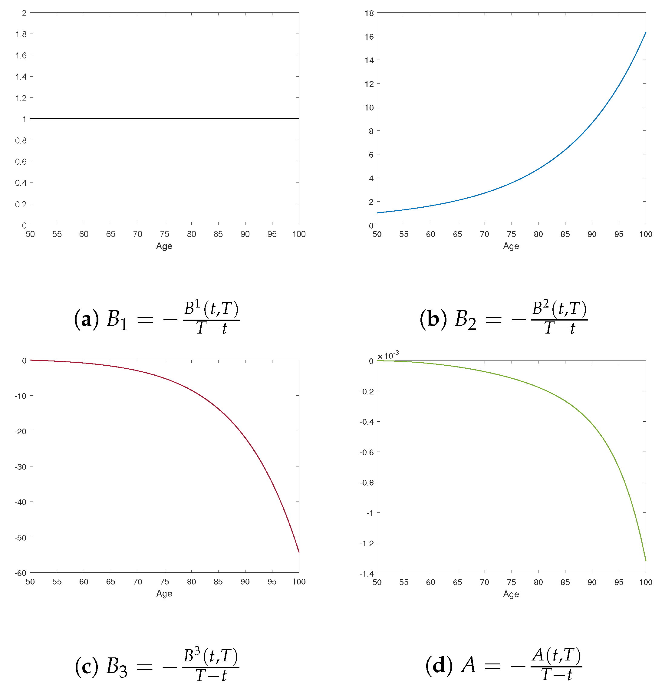
The estimated latent factors and factor loadings for the CIR mortality model are shown in Figure 5 and Figure 6. As expected, the factors and factor loadings differ from those of the independent AFNS mortality model, reflecting the different model assumptions.
The first factor X 1 is relatively stable for cohorts born before 1900, then increases, followed by a moderate decline for cohorts born around 1910 and after. The factor loading, B 1 , is positive and increases with age. The interaction between the factor dynamics and the factor loading for the first factor X 1 results in older ages in the age-cohort mortality curve being affected more by the first factor than for younger ages. Since X 1 is the largest factor throughout the time period and the factor loadings are largest for this factor, it is the dominant factor impacting changes in mortality in the CIR model.
The second factor X 2 has a downward trend over time. The factor loading B 2 is decreasing with age and smaller than B 1 . As a result, younger ages have mortality improvement from the second factor, but the size of improvement from this factor is smaller than for the first factor. As a result, it has a much smaller overall impact compared to X 1 .
The third factor X 3 is relatively constant for cohorts born before 1900, decreasing afterwards, with a reduction in the rate of decrease for cohorts born after around 1910. The factor loading B 3 has a convex shape, is positive, and impacts older ages more than younger ages. This results in curvature changes in the age-cohort survival curve.
The adjustment term A, which produces the consistency in the age-cohort survival curves, is negative and, following a small increase for younger ages, is then decreasing.
The combination of the factor dynamics for all the factor dynamics along with the factor loadings determine the shape and dynamics of the age-cohort survival curves. These dynamics are estimated from the age-cohort mortality data and allow an analysis of the underlying trends and changes in the age-cohort survival curve over time. The more complex dynamics than single factor models explain the variation at older ages better.

4.5. Residual Analysis

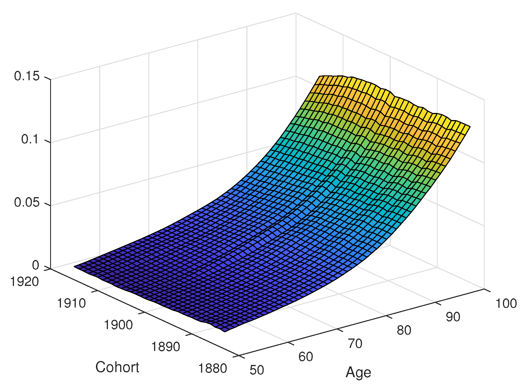
The residuals or the affine mortality models are shown in Figure 7. The residuals shown are the differences between the average force of mortality from the historical mortality data and those determined from the fitted mortality models. Plots are on the same scale on the z-axis, except for the independent Blackburn–Sherris model, which has large residuals at older ages, reflecting a poorer fit at these ages.
Excluding the independent Blackburn–Sherris model, all of the other affine age-cohort mortality models show similar residuals. With three factors for level, slope, and curvature, we see that the independent AFNS model (Figure 7c) fits well. The AFNS model reduces the magnitude of residuals at the older ages compared to the independent Blackburn–Sherris model without adding additional parameters. This shows how, by using factors for level, slope, and curvature factors, the mortality model can capture variation in mortality curves, especially at older ages.
We see how factor dependence in the Blackburn–Sherris model produces a better fitting model, reducing the size of residuals, and accounting better for mortality variation at older ages. This is seen by comparing the dependent Blackburn–Sherris model (Figure 7b) with the independent model (Figure 7a). Although including dependence in the factors of the Blackburn–Sherris model improves the residuals of the model fit, we do not see this for the independent AFNS model in Figure 7c. The residuals in the dependent AFNS model (Figure 7d) are larger, particularly at older ages. This highlights how the independent AFNS model captures mortality variability better than the dependent AFNS model, in contrast to the dependent Blackburn–Sherris model.
The CIR model has lower residuals at older ages and residuals similar to those of the independent AFNS model in Figure 7c. The CIR model has slightly smaller residuals at older ages and ages younger than 60, compared with the other models.
We see a hump shape running diagonally across the cohorts in all of the residual plots. Diagonal effects in an age-cohort model correspond to period effects. The residuals highlight a period mortality effect that impacts all of the cohorts around the year 1970. This corresponds to when period mortality improvement trends in age-period models showed a change to a higher level of improvement. We also see that for later cohorts at older ages, the residuals are higher, which would be indicative of a slowing of mortality-improvement rates in recent years.

4.6. In-Sample Analysis

We now consider an in-sample model performance analysis. We compare estimated cohort survival probabilities from the fitted mortality models with the cohort survival probabilities from the historical data. 
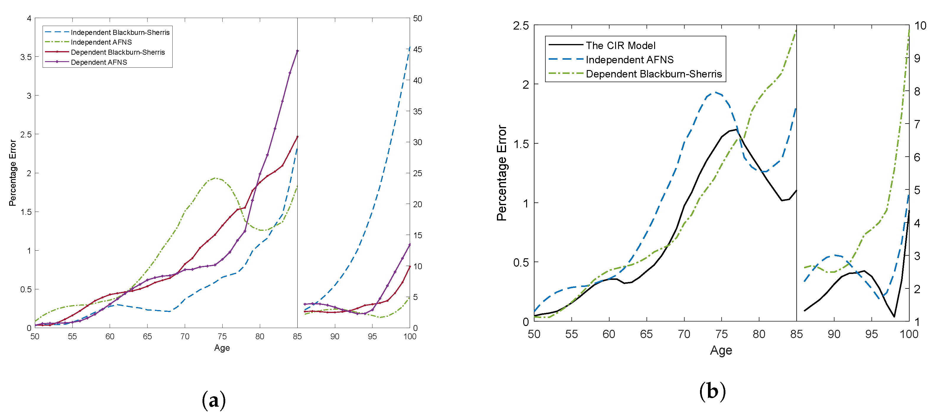
Figure 8 summarizes the in-sample model fit using the Mean Absolute Percentage Error (MAPE) for each age across all cohorts. The scale of the percentage error is different above and below age 85 because of the significant differences in the size of the errors.
Figure 8a shows the MAPE for the affine mortality models with Gaussian processes. Below age 85, all models have similar performance, and the differences between the percentage errors of the different mortality models are relatively small. What is more interesting is the fit above age 85. The independent Blackburn–Sherris model has significantly larger percentage errors. The other affine age-cohort Gaussian mortality models, the dependent Blackburn–Sherris model and the independent AFNS model, have similar and improved model fit at these older ages.
We compare the MAPE of these better performing Gaussian mortality models with the CIR age-cohort mortality model in Figure 8b. We see that the CIR mortality model and the independent AFNS mortality model are similar. The latter has only slightly larger percentage errors at most ages. The dependent Blackburn–Sherris model is similar to the CIR model below age 75, but the percentage errors increase after age 75 with values as high as 10%.
Based on MAPE, we see that both the independent AFNS mortality model and the CIR mortality model have similar and satisfactory performance for the historical age-cohort data for complete cohorts in the USA historical mortality.

5. Forecasts of Survival Probabilities

We compare the predictive performance of the affine mortality models using an out-of-sample forecast with the fitted parameter values estimated from the cohorts born 1883 to 1915 for ages 50 to 100 used to forecast the survival curve of the cohort born in 1916. For this cohort we have full historical mortality data.
Following Christensen et al. (2011), who use optimal forecasts to predict yields to maturity, we use optimal forecasts, also referred to as best-estimate forecasts, to project average forces of mortality and survival probabilities.
At time t, the average force of mortality over τ = T + 1 t + 1 periods at time t + 1 for cohort i, μ ¯ i t + 1 , T + 1 , is
μ ¯ i t + 1 , T + 1 = B t , T T t E X t + 1 | X t A t , T T t ,
where B t , T and A t , T only depend on τ = T t .
The forecasts of survival probabilities are then
S t + 1 , T + 1 = exp B t , T E X t + 1 | X t + A t , T .
Since the factor dynamics under measure P in the independent Blackburn–Sherris model and the three-factor independent AFNS model are the same, the conditional expectations of state variables for these two models are as follows:
E X t + 1 1 | X t 1 = e k 11 P X t 1 , E X t + 1 2 | X t 2 = e k 22 P X t 2 , E X t + 1 3 | X t 3 = e k 33 P X t 3 .
For the independent AFNS model, the conditional mean has the same structure but with X t = L t , S t , C t .
The SDEs describing the P-dynamics of the dependent Blackburn–Sherris model and the dependent AFNS model are the same as for the independent factor model in Equation (47).
The conditional mean of the CIR model is given in Geyer and Pichler (1999), so for the mortality model:
E X t + 1 1 | X t 1 = e k 11 P X t 1 + θ 1 P 1 e k 11 P , E X t + 1 2 | X t 2 = e k 22 P X t 2 + θ 2 P 1 e k 22 P , E X t + 1 3 | X t 3 = e k 33 P X t 3 + θ 3 P 1 e k 33 P .
The RMSE under each mortality model for projecting the 1916 cohort survival curve are shown in Table 4. We see that the independent AFNS mortality model performs best on these criteria. The dependent AFNS mortality model and the dependent Blackburn–Sherris models perform similarly. In contrast, the independent Blackburn–Sherris mortality model shows the poorest performance. Although the CIR mortality model has reasonable RMSE, it is outperformed by the AFNS mortality models.
To illustrate these differences, Figure 9 shows the survival probabilities for the different mortality models using the best estimate forecasts compared to the actual survival probabilities from the historical mortality data. The models produce reasonable survival curve fits, except the independent Blackburn–Sherris mortality model and the CIR mortality model, which both underestimate the survival rates of the 1916 cohort.
Figure 10 shows the absolute percentage errors across ages for all the mortality models. This confirms the better forecasting performance of the independent AFNS mortality model. The dependent Blackburn–Sherris mortality models performs better than the independent Blackburn–Sherris mortality model, showing the benefit in forecasting of including correlations between the factors in this model. The level, slope, and curvature structure of the factors in the AFNS mortality model reduce the need for including dependence in the factors as compared to the Blackburn–Sherris mortality model.

6. Discussion

We have shown how affine mortality models can be applied to age-cohort mortality data using USA mortality data. We show that three-factor versions of these models fit the data well; the Gaussian models produce low probabilities of negative mortality rates; and the AFNS model, with level, slope, and curvature as factors, provides reliable forecasts of full age-cohort survival curves. We model age-cohort data since age-cohort survival curves are required for practical actuarial applications. Most other research uses age-period mortality, often with a cohort effect adjustment. Our analysis has used USA mortality data since the population is large and reflects many developments in mortality improvement expected to be found in other developed countries.
We develop our models in an arbitrage-free pricing framework assuming independence between interest rates and mortality. Correlation between interest rates and mortality rates can be incorporated into the models by an appropriate change in measure. Calibrating the models and estimating the correlation between interest rates and mortality rates would then require mortality-linked security prices that capture both interest rate and mortality risk.
Our results provide interesting insights into age-cohort mortality curve dynamics. Although we have focused on USA data, estimating and comparing age-cohort affine mortality models for other countries will provide a deeper understanding of the models and their ability to capture differing mortality dynamics.
There are a number of directions for which this research provides a foundation. We use the Kalman filter with maximum likelihood to estimate parameters. An area of research that would improve the model estimation is the development of efficient numerical estimation processes for the Kalman filter along with developing code that can be used by other researchers to estimate and implement the models.
We use only historical data for complete cohorts in our age-cohort mortality curve modelling. Incorporating incomplete cohorts into the estimation will allow the use of more recent age-cohort data in the model estimation and forecasting. Age-period data use the latest calendar year mortality data, whereas age-cohort data for later calendar years are incomplete.
We do not focus on parameter stability, and although this has been considered in (Blackburn and Sherris 2013), assessing this for several other countries would provide additional support for the empirical performance of the multi-factor affine models.
Although we include dependence between the factors by incorporating correlation, we do not include age effects in the factors. In the affine framework, it is possible to capture age dependence in the factors to improve the model fit at older ages with potentially fewer factors in the model. It is also possible to capture age correlations and cohort correlations more effectively using age-dependent factors.
An important issue to also consider is the extension of the models to incorporate jump events such as the COVID-19 pandemic. These events not only have an impact on all ages to a greater or lesser extent in a particular number of periods, but can also have longer lasting impacts, as is occurring with long COVID-19. The affine models we consider do not account for larger jumps that impact several periods across all ages, as would be the case for a pandemic. The models can incorporate jumps such as COVID-19 into the affine mortality framework.
These extensions are all topics that current CEPAR actuarial research is investigating.

7. Conclusions

We have applied several continuous-time affine mortality models to age-cohort survival curve data using USA historical age-cohort data to fit and assess the mortality models. We provide a comprehensive analysis and comparison of the models. We outline, compare, and assess several independent-factor and dependent-factor affine mortality models with Gaussian processes, including the Blackburn–Sherris mortality model (Blackburn and Sherris 2013; Christensen et al. 2011), as well as an affine mortality model with square-root processes (the CIR mortality model). The CIR mortality model precludes negative mortality rates that can occur in the Gaussian models. The CIR latent factors and the mortality intensity have non-central Chi-square distributions, which can better reflect mortality heterogeneity. We also assess the performance of an AFNS mortality model with interpretable latent stochastic factors for level, slope, and curvature of the survival curve.
We incorporate dependence in the Blackburn–Sherris mortality model by including correlation between the factors and show how this improves in-sample model fit and out-of-sample forecasting performance. The CIR mortality model shows the best in-sample model fit across a range of criteria, including model residuals. The superior in-sample performance of the CIR mortality model is likely to reflect the more realistic assumption of Gamma-distributed mortality rates compared to the Gaussian models.
We find that the independent-factor AFNS mortality model performs well. It better captures the variation in age-cohort mortality rates in USA data and produces a better fit at older ages than the independent-factor Blackburn–Sherris model. Negative mortality rates have very low probability in the AFNS mortality models.
We project a complete cohort based on the fitted models to assess forecasting performance of the models. We forecast the 1916 cohort in the USA data, for which we have a complete cohort of mortality data. The independent-factor AFNS mortality model shows better predictive performance compared to the other models.
Based on our detailed assessment and comparison of these affine age-cohort mortality models, we show that, for USA age-cohort mortality data, the independent AFNS model provides satisfactory model fit and satisfactory predictive performance. The model is parsimonious relative to other models and can be readily estimated using the Kalman filter, allowing for Poisson mortality variation in the measurement equation. The model has intuitive factor interpretations in terms of level, slope, and curvature for the dynamics of the mortality survival curve and is well suited for financial and insurance applications, including pricing and longevity risk management.

Author Contributions

Conceptualization, Z.H. and M.S.; methodology, Z.H. and M.S.; software, Z.H.; validation, Z.H., M.S., A.M.V. and J.Z.; formal analysis, Z.H.; investigation, Z.H.; writing—original draft preparation, Z.H.; writing—review and editing, M.S., A.M.V. and J.Z.; supervision, M.S., A.M.V. and J.Z.; funding acquisition, M.S., A.M.V. and J.Z. All authors have read and agreed to the published version of the manuscript.

Funding

This research received financial support from the Society of Actuaries Center of Actuarial Excellence Research Grant 2017–2020: Longevity Risk: Actuarial and Predictive Models, Retirement Product Innovation, and Risk Management Strategies, as well as support from CEPAR Australian Research Council Centre of Excellence in Population Ageing Research project number CE170100005.

Institutional Review Board Statement

Not applicable.

Informed Consent Statement

Not applicable.

Data Availability Statement

We used publicly available data in this study. The mortality data for USA are available on the Human Mortality Database (https://www.mortality.org/, accessed on 18 October 2018).

Conflicts of Interest

The authors declare no conflict of interest.

Appendix A. Solutions to the Ordinary Differential Equations

We have
d d t e K Q T t B t , T = e K Q T t d B t , T d t K Q e K Q T t B t , T ,
and substituting Equation (7), we simplify to obtain
t T d d s e K Q T s B s , T d s = t T e K Q T s ρ 1 d s ,
which has the solution, after including the boundary conditions,
B t , T = e K Q T t t T e K Q T s ρ 1 d s .
With K Q in Equation (18) and ρ 1 = 1 , 1 , 1 T in the Blackburn–Sherris model,
e K Q T s ρ 1 = a 11 a 21 a 31 0 a 22 a 32 0 0 a 33 1 1 1 = a 11 + a 21 + a 31 a 22 + a 32 a 33
where
a 11 = e δ 11 T s , a 21 = D 1 e δ 11 T s e δ 22 T s , a 31 = D 4 + D 1 D 5 e δ 11 T s D 1 D 2 e δ 22 T s + D 2 D 3 D 4 e δ 33 T s , a 22 = e δ 22 T s , a 32 = D 2 e δ 22 T s e δ 33 T s , a 33 = e δ 33 T s ,
and
D 1 = δ 21 δ 11 δ 22 , D 2 = δ 32 δ 22 δ 33 , D 3 = δ 21 δ 11 δ 33 , D 4 = δ 31 δ 11 δ 33 , D 5 = δ 32 δ 11 δ 33 .
Integrating each element in Equation (A4),
b 1 = t T a 11 + a 21 + a 31 d s = 1 + D 1 + D 1 D 5 + D 4 1 e δ 11 T t δ 11 D 1 1 + D 2 1 e δ 22 T t δ 22 + D 2 D 3 D 4 1 e δ 33 T t δ 33 , b 2 = t T a 22 + a 32 d s = 1 + D 2 1 e δ 22 T t δ 22 D 2 1 e δ 33 T t δ 33 , b 3 = t T a 33 d s = 1 e δ 33 T t δ 33 .
Let
e K Q T t = c 11 c 21 c 31 0 c 22 c 32 0 0 c 33 ,
where
c 11 = e δ 11 T t , c 21 = D 1 e δ 11 T t e δ 22 T t , c 31 = D 4 + D 1 D 5 e δ 11 T t D 1 D 2 e δ 22 T t + D 2 D 3 D 4 e δ 33 T t , c 22 = e δ 22 T t , c 32 = D 2 e δ 22 T t e δ 33 T t , c 33 = e δ 33 T t .
Equation (A3) now can be written as:
B 1 t , T B 2 t , T B 3 t , T = c 11 c 21 c 31 0 c 22 c 32 0 0 c 33 b 1 b 2 b 3 .
Therefore, the solutions of B t , T are
B 1 t , T = E 1 1 e δ 11 T t δ 11 + E 2 1 e δ 22 T t δ 22 E 3 1 e δ 33 T t δ 33 , B 2 t , T = 1 + D 2 1 e δ 22 T t δ 22 + D 2 1 e δ 33 T t δ 33 , B 3 t , T = 1 e δ 33 T t δ 33 ,
where E 1 = 1 + D 1 + D 1 D 5 + D 4 , E 2 = D 1 1 + D 2 , E 3 = D 2 D 3 D 4 .
From Equation (8) and the boundary condition,
A t , T = 1 2 t T j = 1 3 Σ B s , T B s , T Σ j , j d s = 1 2 t T σ 11 2 B 1 s , T 2 + σ 21 2 + σ 22 2 B 2 s , T 2 + σ 31 2 + σ 32 2 + σ 33 2 B 3 s , T 2 + 2 σ 11 σ 21 B 1 s , T B 2 s , T + 2 σ 11 σ 31 B 1 s , T B 3 s , T + 2 σ 21 σ 31 + σ 22 σ 32 B 2 s , T B 3 s , T d s .
Terms with B s , T are expanded as follows:
B 1 s , T 2 = E 1 2 δ 11 2 1 e δ 11 T s 2 + E 2 2 δ 22 2 1 e δ 22 T s 2 + E 3 2 δ 33 2 1 e δ 33 T s 2 2 δ 11 δ 22 E 1 E 2 1 e δ 11 T s 1 e δ 22 T s + 2 δ 11 δ 33 E 1 E 3 1 e δ 11 T s 1 e δ 33 T s 2 δ 22 δ 33 E 2 E 3 1 e δ 22 T s 1 e δ 33 T s ,
B 2 s , T 2 = 1 + D 2 2 δ 22 2 1 e δ 22 T s 2 + D 2 2 δ 33 2 1 e δ 33 T s 2 2 δ 22 δ 33 D 2 1 + D 2 1 e δ 22 T s 1 e δ 33 T s ,
B 3 s , T 2 = 1 δ 33 2 1 e δ 33 T s 2 ,
B 1 s , T B 2 s , T = E 1 1 + D 2 δ 11 δ 22 1 e δ 11 T s 1 e δ 22 T s E 1 D 2 δ 11 δ 33 1 e δ 11 T s 1 e δ 33 T s + 1 δ 22 δ 33 E 2 D 2 + E 3 1 + D 2 1 e δ 22 T s 1 e δ 33 T s E 2 1 + D 2 δ 22 2 1 e δ 22 T s 2 E 3 D 2 δ 33 2 1 e δ 33 T s 2 ,
B 1 s , T B 3 s , T = E 1 δ 11 δ 33 1 e δ 11 T s 1 e δ 33 T s + E 3 δ 33 2 1 e δ 33 T s 2 E 2 δ 22 δ 33 1 e δ 22 T s 1 e δ 33 T s ,
B 2 s , T B 3 s , T = 1 + D 2 δ 22 δ 33 1 e δ 22 T s 1 e δ 33 T s D 2 δ 33 2 1 e δ 33 T s 2 .
Collecting terms with 1 e δ j j T s 2 and 1 e δ i i T s 1 e δ j j T s ( i , j = 1 , 2 , 3 and i j ) and integrating,
A t , T = 1 2 F 1 δ 11 3 1 2 1 e 2 δ 11 T t 2 1 e δ 11 T t + δ 11 T t + F 2 δ 22 3 1 2 1 e 2 δ 22 T t 2 1 e δ 22 T t + δ 22 T t + F 3 δ 33 3 1 2 1 e 2 δ 33 T t 2 1 e δ 33 T t + δ 33 T t + F 4 δ 11 δ 22 T t 1 e δ 11 T t δ 11 1 e δ 22 T t δ 22 1 e δ 11 + δ 22 T t δ 11 + δ 22 + F 5 δ 11 δ 33 T t 1 e δ 11 T t δ 11 1 e δ 33 T t δ 33 1 e δ 11 + δ 33 T t δ 11 + δ 33 + F 6 δ 22 δ 33 T t 1 e δ 22 T t δ 22 1 e δ 33 T t δ 33 1 e δ 22 + δ 33 T t δ 22 + δ 33 ,
where
F 1 = σ 11 2 E 1 2 , F 2 = σ 11 2 E 2 2 2 σ 11 σ 21 E 2 1 + D 2 + σ 21 2 + σ 22 2 1 + D 2 2 , F 3 = σ 11 2 E 3 2 2 σ 11 σ 21 E 3 D 2 + σ 21 2 + σ 22 2 D 2 2 2 σ 21 σ 31 + σ 22 σ 32 D 2 + 2 σ 11 σ 31 E 3 + σ 31 2 + σ 32 2 + σ 33 2 , F 4 = 2 σ 11 2 E 1 E 2 + 2 σ 11 σ 21 E 1 1 + D 2 , F 5 = 2 σ 11 2 E 1 E 3 2 σ 11 σ 21 E 1 D 2 + 2 σ 11 σ 31 E 1 , F 6 = 2 σ 11 2 E 2 E 3 + 2 σ 11 σ 21 E 3 1 + D 2 + E 2 D 2 2 σ 11 σ 31 E 2 + 2 σ 21 σ 31 + σ 22 σ 32 1 + D 2 2 σ 21 2 + σ 22 2 D 2 1 + D 2 .

Appendix B. Real World Dynamics and Change of Measure

Appendix B.1. Models with Gaussian Processes

The market price of risk has the following form:
Λ t = λ 0 + λ 1 X t ,
where Λ t R n × 1 , λ 0 R n × 1 and λ 1 R n × n .
With the above specification, the SDEs of the state variables X t under the real-world measure P are derived as follows:
d X t = K Q θ Q X t d t + Σ d W t P + Λ t d t = K Q θ Q X t d t + Σ λ 0 d t + λ 1 X t d t + d W t P d t = K Q θ Q + Σ λ 0 d t K Q Σ λ 1 X t d t + Σ d W t P = K Q Σ λ 1 K Q θ Q + Σ λ 0 K Q Σ λ 1 X t d t + Σ d W t P = K P θ P X t d t + Σ d W t P ,
where
K P = K Q Σ λ 1 , θ P = K Q θ Q + Σ λ 0 K Q .

Appendix B.2. The CIR Model

Following the essentially affine model structure in Duffee (2002), the market price of longevity risk for the multi-factor CIR model is specified as:
Λ t = D X t , t λ 0 = X t 1 0 0 0 X t 2 0 0 0 X t 3 λ 1 0 λ 2 0 λ 3 0 ,
where Λ t R 3 × 1 represents risk premium and λ 0 R 3 × 1 , and let
D 2 X t , t λ 0 = X t 1 0 0 0 X t 2 0 0 0 X t 3 X t 1 0 0 0 X t 2 0 0 0 X t 3 λ 1 0 λ 2 0 λ 3 0 = X t 1 0 0 0 X t 2 0 0 0 X t 3 λ 1 0 λ 2 0 λ 3 0 = λ 1 0 X t 1 λ 2 0 X t 2 λ 3 0 X t 3 = λ 1 0 0 0 0 λ 2 0 0 0 0 λ 3 0 X t 1 X t 2 X t 3 = Λ 0 X t .
The SDEs of the state variables X t under the real-world measure P are derived as following
d X t = K Q θ Q X t d t + Σ D X t , t d W t P + Λ t d t = K Q θ Q X t d t + Σ D X t , t D X t , t λ 0 d t + d W t P d t = K Q θ Q K Q X t + Σ D 2 X t , t λ 0 d t + Σ D X t , t d W t P = K Q θ Q K Q Σ Λ 0 X t d t + Σ D X t , t d W t P = K Q Σ Λ 0 K Q θ Q K Q Σ Λ 0 X t d t + Σ D X t , t d W t P = K P θ P X t d t + Σ D X t , t d W t P ,
where
K P = K Q Σ Λ 0 , θ P = K Q θ Q K Q Σ Λ 0 .

References

  1. Alai, Daniel, Katja Ignatieva, and Michael Sherris. 2019. The investigation of a forward-rate mortality framework. Risks 7: 61. [Google Scholar] [CrossRef]
  2. Barrieu, Pauline, Harry Bensusan, Nicole El Karoui, Caroline Hillairet, Stéphane Loisel, Claudia Ravanelli, and Yahia Salhi. 2012. Understanding, modelling and managing longevity risk: Key issues and main challenges. Scandinavian Actuarial Journal 2012: 203–31. [Google Scholar] [CrossRef]
  3. Bauer, Daniel, Matthias Börger, Jochen Ruß, and Hans-Joachim Zwiesler. 2008. The volatility of mortality. Asia-Pacific Journal of Risk and Insurance 3. [Google Scholar] [CrossRef]
  4. Biffis, Enrico. 2005. Affine processes for dynamic mortality and actuarial valuations. Insurance: Mathematics and Economics 37: 443–68. [Google Scholar] [CrossRef]
  5. Björk, Tomas, and Bent Jesper Christensen. 1999. Interest rate dynamics and consistent forward rate curves. Mathematical Finance 9: 323–48. [Google Scholar] [CrossRef]
  6. Blackburn, Craig, and Michael Sherris. 2013. Consistent dynamic affine mortality models for longevity risk applications. Insurance: Mathematics and Economics 53: 64–73. [Google Scholar] [CrossRef]
  7. Blake, David, Tom Boardman, and Andrew Cairns. 2014. Sharing longevity risk: Why governments should issue longevity bonds. North American Actuarial Journal 18: 258–77. [Google Scholar] [CrossRef]
  8. Blake, David, and William Burrows. 2001. Survivor bonds: Helping to hedge mortality risk. Journal of Risk and Insurance 68: 339–48. [Google Scholar] [CrossRef]
  9. Blake, David, Nicole El Karoui, Stéphane Loisel, and Richard MacMinn. 2018. Longevity risk and capital markets: The 2015–16 update. Insurance: Mathematics and Economics 78: 157–73. [Google Scholar] [CrossRef]
  10. Cairns, Andrew J. G., David Blake, and Kevin Dowd. 2006a. Pricing death: Frameworks for the valuation and securitization of mortality risk. ASTIN Bulletin 36: 79–120. [Google Scholar] [CrossRef] [Green Version]
  11. Cairns, Andrew J. G., David Blake, and Kevin Dowd. 2006b. A two-factor model for stochastic mortality with parameter uncertainty: Theory and calibration. Journal of Risk and Insurance 73: 687–718. [Google Scholar] [CrossRef]
  12. Cairns, Andrew J. G., David Blake, Kevin Dowd, Guy D. Coughlan, David Epstein, Alen Ong, and Igor Balevich. 2009. A quantitative comparison of stochastic mortality models using data from England and Wales and the United States. North American Actuarial Journal 13: 1–35. [Google Scholar] [CrossRef]
  13. Chang, Yang, and Michael Sherris. 2018. Longevity Risk Management and the Development of a Value-Based Longevity Index. Risks 6: 10. [Google Scholar] [CrossRef]
  14. Chen, Ren-Raw, and Louis Scott. 2003. Multi-factor Cox-Ingersoll-Ross models of the term structure: Estimates and tests from a Kalman filter model. The Journal of Real Estate Finance and Economics 27: 143–72. [Google Scholar] [CrossRef]
  15. Christensen, Jens H. E., Francis X. Diebold, and Glenn D. Rudebusch. 2011. The affine arbitrage-free class of Nelson–Siegel term structure models. Journal of Econometrics 164: 4–20. [Google Scholar] [CrossRef]
  16. Continuous Mortality Investigation. 2018. The CMI Mortality Projections Model, CMI2017. Working paper. London: The Institute and Faculty of Actuaries. [Google Scholar]
  17. Coughlan, Guy, David Epstein, Amit Sinha, and Paul Honig. 2007. q-Forwards: Derivatives for Transferring Longevity and Mortality Risks. London: JPMorgan Pension Advisory Group. [Google Scholar]
  18. Cox, John C., Jonathan E. Ingersoll, and Stephen A. Ross. 1985. A theory of the term structure of interest rates. Econometrica 53: 385–407. [Google Scholar] [CrossRef]
  19. Dahl, Mikkel. 2004. Stochastic mortality in life insurance: Market reserves and mortality-linked insurance contracts. Insurance: Mathematics and Economics 35: 113–36. [Google Scholar] [CrossRef]
  20. Dahl, Mikkel, and Thomas Møller. 2006. Valuation and hedging of life insurance liabilities with systematic mortality risk. Insurance: Mathematics and Economics 39: 193–217. [Google Scholar] [CrossRef]
  21. Dai, Qiang, and Kenneth J. Singleton. 2000. Specification analysis of affine term structure models. The Journal of Finance 55: 1943–978. [Google Scholar] [CrossRef]
  22. De Rossi, Giuliano. 2004. Kalman filtering of consistent forward rate curves: A tool to estimate and model dynamically the term structure. Journal of Empirical Finance 11: 277–308. [Google Scholar] [CrossRef]
  23. Diebold, Francis X., and Canlin Li. 2006. Forecasting the term structure of government bond yields. Journal of Econometrics 130: 337–64. [Google Scholar] [CrossRef]
  24. Diebold, Francis X., and Glenn D. Rudebusch. 2013. Yield Curve Modeling and Forecasting: The Dynamic Nelson-Siegel Approach. Princeton: Princeton University Press. [Google Scholar]
  25. Dowd, Kevin, David Blake, Andrew J. G. Cairns, and Paul Dawson. 2006. Survivor swaps. Journal of Risk and Insurance 73: 1–17. [Google Scholar] [CrossRef]
  26. Duan, Jin-Chuan, and Jean-Guy Simonato. 1999. Estimating and testing exponential-affine term structure models by Kalman filter. Review of Quantitative Finance and Accounting 13: 111–35. [Google Scholar] [CrossRef]
  27. Duffee, Gregory R. 2002. Term premia and interest rate forecasts in affine models. The Journal of Finance 57: 405–43. [Google Scholar] [CrossRef]
  28. Duffie, Darrell, and Rui Kan. 1996. A yield-factor model of interest rates. Mathematical Finance 6: 379–406. [Google Scholar] [CrossRef]
  29. Durbin, James, and Siem Jan Koopman. 2012. Time Series Analysis by State Space Methods. Oxford: Oxford University Press, vol. 38. [Google Scholar]
  30. Gallop, Adrian. 2008. Mortality projections in the United Kingdom. In Society of Actuaries Living to 100 Symposium. Chicago: Society of Actuaries. [Google Scholar]
  31. Geyer, Alois L. J., and Stefan Pichler. 1999. A state-space approach to estimate and test multifactor Cox-Ingersoll-Ross models of the term structure. Journal of Financial Research 22: 107–30. [Google Scholar] [CrossRef]
  32. Human Mortality Database. 2018. U.S.A. Life Tables. University of California, Berkeley (USA), and Max Planck Institute for Demographic Research (Germany). Available online: http://www.mortality.org/cgi-bin/hmd/country.php?cntr=USA&level=1 (accessed on 18 October 2018).
  33. Jevtic, Petar, Elisa Luciano, and Elena Vigna. 2013. Mortality surface by means of continuous time cohort models. Insurance: Mathematics and Economics 53: 122–33. [Google Scholar] [CrossRef]
  34. Jevtić, Petar, and Luca Regis. 2019. A continuous-time stochastic model for the mortality surface of multiple populations. Insurance: Mathematics and Economics 88: 181–95. [Google Scholar] [CrossRef]
  35. Jevtić, Petar, and Luca Regis. 2021. A square-root factor-based multi-population extension of the mortality laws. Mathematics 9: 2402. [Google Scholar] [CrossRef]
  36. Lee, Ronald D., and Lawrence R. Carter. 1992. Modeling and forecasting U.S. mortality. Journal of the American Statistical Association 87: 659–71. [Google Scholar] [CrossRef]
  37. Life and Longevity Markets Association. 2010. Longevity Pricing Framework: Framework for Pricing Longevity Exposures Developed by the LLMA (Life and Longevity Markets Association). Technical Report. London: Life and Longevity Markets Association. [Google Scholar]
  38. Luciano, Elisa, Jaap Spreeuw, and Elena Vigna. 2008. Modelling Stochastic Mortality for Dependent Lives. Insurance: Mathematics and Economics 43: 234–44. [Google Scholar] [CrossRef]
  39. Milevsky, Moshe A., and S. David Promislow. 2001. Mortality derivatives and the option to annuitise. Insurance: Mathematics and Economics 29: 299–318. [Google Scholar] [CrossRef]
  40. Novokreshchenova, Anastasia. 2016. Predicting human mortality: Quantitative evaluation of four stochastic models. Risks 4: 45. [Google Scholar] [CrossRef]
  41. Pitacco, Ermanno. 2016. High Age Mortality and Frailty. Some Remarks and Hints for Actuarial Modeling. Available online: http://www.cepar.edu.au/working-papers/working-papers-2016.aspx (accessed on 1 September 2022).
  42. Renshaw, Arthur, and Steven Haberman. 2006. A cohort-based extension to the Lee–Carter model for mortality reduction factors. Insurance: Mathematics and Economics 38: 556–70. [Google Scholar] [CrossRef]
  43. Schrager, David F. 2006. Affine stochastic mortality. Insurance: Mathematics and Economics 38: 81–97. [Google Scholar] [CrossRef]
  44. Shumway, Robert H., and David S. Stoffer. 2017. Time Series Analysis and Its Applications. Berlin/Heidelberg: Springer. [Google Scholar]
  45. SriDaran, Dilan, Michael Sherris, Andrés M. Villegas, and Jonathan Ziveyi. 2022. A group regularisation approach for constructing generalised age-period-cohort mortality projection models. ASTIN Bulletin 52: 247–89. [Google Scholar] [CrossRef]
  46. The Joint Forum. 2013. Longevity Risk Transfer Markets: Market Structure, Growth Drivers and Impediments, and Potential Risks. Technical Report. Available online: https://www.bis.org/publ/joint34.htm (accessed on 1 September 2022).
  47. Willets, Richard C. 2004. The cohort effect: Insights and explanations. British Actuarial Journal 10: 833–77. [Google Scholar] [CrossRef]
  48. Xu, Yajing, Michael Sherris, and Jonathan Ziveyi. 2020a. Continuous-time multi-cohort mortality modelling with affine processes. Scandinavian Actuarial Journal 2020: 526–52. [Google Scholar] [CrossRef]
  49. Xu, Yajing, Michael Sherris, and Jonathan Ziveyi. 2020b. Market price of longevity risk for a multi-cohort mortality model with application to longevity bond option pricing. Journal of Risk and Insurance 87: 571–95. [Google Scholar] [CrossRef]
Figure 1. Average Force of Mortality for Males Born from 1883 to 1915.
Risks 10 00183 g001
Figure 2. Fractions (%) of Variance Explained by Each of the First 7 Principal Components.
Risks 10 00183 g002
Figure 3. Factors in the Independent AFNS Model.
Risks 10 00183 g003
Figure 4. Factor Loadings in the Independent AFNS Model.
Risks 10 00183 g004
Figure 5. Factors in the CIR Model.
Risks 10 00183 g005
Figure 6. Factors Loadings in the CIR Model.
Risks 10 00183 g006
Figure 7. Residuals of Affine Mortality Models.
Risks 10 00183 g007
Figure 8. MAPE of Affine Mortality Models. (a) The Models with Gaussian Processes. (b) The CIR Model, the Dependent Blackburn–Sherris Model and the Independent AFNS Model.
Risks 10 00183 g008
Figure 9. Actual and Best-Estimate Survival Probabilities of the 1916 Cohort.
Risks 10 00183 g009
Figure 10. Absolute Percentage Errors between Actual and Best-Estimate Survival Probabilities.
Risks 10 00183 g010
Table 1. Affine Mortality Models—Independent Factor Model Specifications.
ModelFactors X t ρ 1 K Q K P Σ
Blackburn–Sherris Model X t 1 X t 2 X t 3 1 1 1 δ 1 0 0 0 δ 2 0 0 0 δ 3 k 1 P 0 0 0 k 2 P 0 0 0 k 3 P σ 11 0 0 0 σ 22 0 0 0 σ 33
AFNS Model L t S t C t 1 1 0 0 0 0 0 δ δ 0 0 δ k 1 P 0 0 0 k 2 P 0 0 0 k 3 P
Table 2. Estimated Parameters.
The Blackburn–Sherris ModelThe AFNS ModelThe CIR Model
Independent FactorDependent FactorIndependent FactorDependent Factor
δ 11
(AFNS: δ )
−0.01106
(0.00123)
−0.20183
( 2.944 × 10 5 )
−0.08348
( 1.580 × 10 4 )
−0.04725
( 8.096 × 10 5 )
−0.09652
( 2.513 × 10 4 )
δ 21 -0.56206
( 4.091 × 10 5 )
---
δ 22 0.07484
(0.00432)
−0.07092
( 1.766 × 10 5 )
--0.12627
( 2.412 × 10 3 )
δ 31 -0.24075
( 1.555 × 10 5 )
---
δ 32 -0.80809
( 4.102 × 10 5 )
---
δ 33 −0.06883
( 2.452 × 10 4 )
0.77825
( 1.461 × 10 5 )
--−0.11153
( 3.060 × 10 4 )
k 11 P 0.38753−0.042480.187930.018100.00077
k 22 P 0.139100.018690.013610.020020.59402
k 33 P 0.007180.018270.027010.049720.06842
σ 11 0.00782 7.557 × 10 11 9.593 × 10 4 0.004000.00265
( 6.894 × 10 5 )
σ 21 -0.01110-−0.00387-
σ 22 0.00125 3.370 × 10 11 1.120 × 10 4 0.000910.02848
( 1.250 × 10 3 )
σ 31 -−0.01190-−0.00183-
σ 32 -0.00047-0.00123-
σ 33 5.409 × 10 4 0.00029 3.549 × 10 5 0.000230.01360
( 9.494 × 10 5 )
r 1 1.071 × 10 11 4.337 × 10 8 1.422 × 10 10 6.272 × 10 8 5.498 × 10 10
r 2 0.377970.113750.177840.10742 6.646 × 10 7
r c 4.360 × 10 8 5.705 × 10 8 4.963 × 10 7 4.636 × 10 13 3.410 × 10 7
The CIR Model
θ 1 Q 0.00080 θ 2 Q 0.01010 θ 3 Q 0.00137
θ 1 P 0.00697 θ 2 P 0.00415 θ 3 P 0.00356
Table 3. Comparison of Affine Mortality Models.
The Blackburn–Sherris ModelThe AFNS ModelThe CIR Model
Independent FactorDependent FactorIndependent FactorDependent Factor
Log Likelihood9896.4199938.6969665.8019887.87810,045.70
RMSE0.00250 7.601 × 10 4 6.856 × 10 4 9.160 × 10 4 5.227 × 10 4
No. of Parameters1218101318
AIC−19,570.837−19,643.392−19,113.602−19,551.757−19,857.40
BIC−18,968.292−19,008.277−18,521.914−18,943.783−19,222.29
Probability of Negative Mortality0.02700 1.011 × 10 32 1.722 × 10 31 4.34 × 10 14 -
Table 4. RMSE by Comparing the Actual and Best-Estimate Survival Probabilities of the 1916 Cohort.
The Blackburn–Sherris ModelThe AFNS ModelThe CIR Model
IndependentDependentIndependentDependent
RMSE0.031970.007260.006680.007540.01835
Publisher’s Note: MDPI stays neutral with regard to jurisdictional claims in published maps and institutional affiliations.

