A New Fourier Approach under the Lee-Carter Model for Incorporating Time-Varying Age Patterns of Structural Changes

Abstract

The prediction of future mortality improvements is of substantial importance for areas such as population projection, government welfare policies, pension planning and annuity pricing. The Lee-Carter model is one of the widely applied mortality models proposed to capture and predict the trend in mortality reductions. However, some studies have identified the presence of structural changes in historical mortality data, which makes the forecasting performance of mortality models sensitive to the calibration period. Although some attention has been paid to investigating the time or period effects of structural shifts, the potential time-varying age patterns are often overlooked. This paper proposes a new approach that applies a Fourier series with time-varying parameters to the age sensitivity factor in the Lee-Carter model to study the evolution of age effects. Since modelling the age effects is separated from modelling the period effects, the proposed model can incorporate these two sources of structural changes into mortality predictions. Our backtesting results suggest that structural shifts are present not only in the Lee-Carter mortality index over time, but also in the sensitivity to those time variations at different ages.

1. Introduction

As a consequence of technological developments and medical advances, human life expectancy has continued to rise in recent decades. There is a need to predict and monitor the evolution of future mortality levels in fields such as pension planning, insurance, public health and government policy. Researchers and practitioners have proposed various mortality forecasting models to accommodate different needs. For instance, Lee and Carter (1992) introduced a parsimonious mortality model with age and time effects, which can readily be estimated using singular vector decomposition. The Lee-Carter model is one of the most popular models in the extrapolative family whose members assume a continuation of past patterns. In the application of such models, the choice of the sample period can have a significant impact on forecast accuracy (Booth et al. 2006).

On the one hand, adopting only the recent data may overlook historical features that are pivotal for prediction. Also, as mortality data are usually available by single year, too short a calibration period may lead to unstable parameter estimates. On the other hand, longer estimation periods do not necessarily produce more accurate forecasts, as there may exist certain structural changes in the sample. In the current literature, time effects in mortality models (e.g., the pace of mortality reductions) are often captured by random walk with drift (RWD), which may not be appropriate in the presence of structural changes (van Berkum et al. 2013). For example, when a RWD is fitted to the mortality index in the Lee-Carter model, the drift term is determined only by the beginning and ending values, ignoring potential signals of structural changes within the sample period. Consequently, the predicted mortality rates will ignore structural shifts that could impact forecast trends, and may yield results that are highly sensitive to the estimation period.

Approaches to incorporate the effect of structural changes can be considered in three broad categories, the regime-switching model, broken-trend stationary (Perron 1989) and difference stationary processes with breakpoints (van Berkum et al. 2013). Milidonis et al. (2011) argued that regime-switching models can be employed to describe different mortality states. Specifically, they allowed the error term of the mortality index in the Lee-Carter model to switch between two states with different means and variances and suggested potential deviations from the normality of the error term. The main criticism of regime-switching models is that one may not expect influences on human mortality from developments such as medical advances to be reversed over time (van Berkum et al. 2013), which makes the model somewhat unrealistic. It is also difficult to estimate the switching frequencies as there are only a few major structural changes in the last century.

The other two categories focus on the existence of potential structural changes and unit roots in the time series processes of mortality models. Sweeting (2011) proposed a broken-trend stationary model to detect multiple structural changes using the Cairns-Blake-Dowd model (Cairns et al. 2006) as a base. Li et al. (2011) applied a trend stationary model to the mortality index in the Lee-Carter model using data from England and Wales and the United States, allowing a structural change to occur at a breakpoint. They also pointed out that this approach produces rather narrow prediction intervals, which may not be adequate to capture uncertainties of future mortality rates. For difference stationary models, the most common choice is a (multi-dimensional) random walk with drift (e.g., Cairns et al. 2009; Dowd et al. 2010). Nonetheless, several studies have expressed concerns about the appropriateness of assuming a constant drift. For instance, O’Hare and Li (2015) applied a random walk with drift process to the mortality index in the Lee-Carter model and detected changes in the drift term over time based on the mortality data of Australia, the Netherlands, the United Kingdom and the United States. Similar to applications of the broken-trend stationary model, multiple breaks are also analyzed under the difference stationary model in van Berkum et al. (2013, 2016).

To date, most attention has been paid to investigating structural shifts via the time effects of mortality models, neglecting the evolution of age effects. It is often assumed that the age response to mortality changes remains constant over time. Carter and Prskawetz (2001) estimated the parameters of the Lee-Carter model using different subsamples with a fixed length. They found that the pattern of age response changed significantly for the Austrian population over the sample period 1947–1999. Nevertheless, their paper did not propose a readily applicable method to predict future age patterns. Li et al. (2013) rotated the shape of the Lee-Carter age response to depict the acceleration (deceleration) of mortality improvements at older (younger) ages. The life expectancy at birth is employed as an indicator for the occurrence of the rotation in age patterns, which involves the projection of future life expectancy. Despite the subtleness of the rotation approach, they emphasized the importance of incorporating the changing age patterns into mortality predictions. In the recent work of Li and Wong (2020), the authors attempted to capture the movements of age patterns by analyzing the age response in the Lee-Carter model from (relatively) homogeneous subperiods. They suggested three ways to estimate future age responses, including assuming a continuation of the latest patterns, fitting a modified Heligman and Pollard (1980) curve and applying principal components analysis. Specifically, estimated parameters of the fitted curve and principal components over successive subperiods can be extrapolated via linear regression to compute the age sensitivity parameter for a future period. Their study emphasized the importance of considering the changing age patterns of structural changes in mortality predictions.

In light of the findings of time-varying age effects, this paper proposes a method to fit and forecast the evolution of the age sensitivity factor under the Lee-Carter model, integrating for the first time structural changes in both age and time effects. The method is applied to mortality data for the male population aged 0 to 89 from 1950 to 20161 of Australia, Canada, New Zealand, Sweden, the United Kingdom and the United States, from the Human Mortality Database (Human Mortality Database 2019).

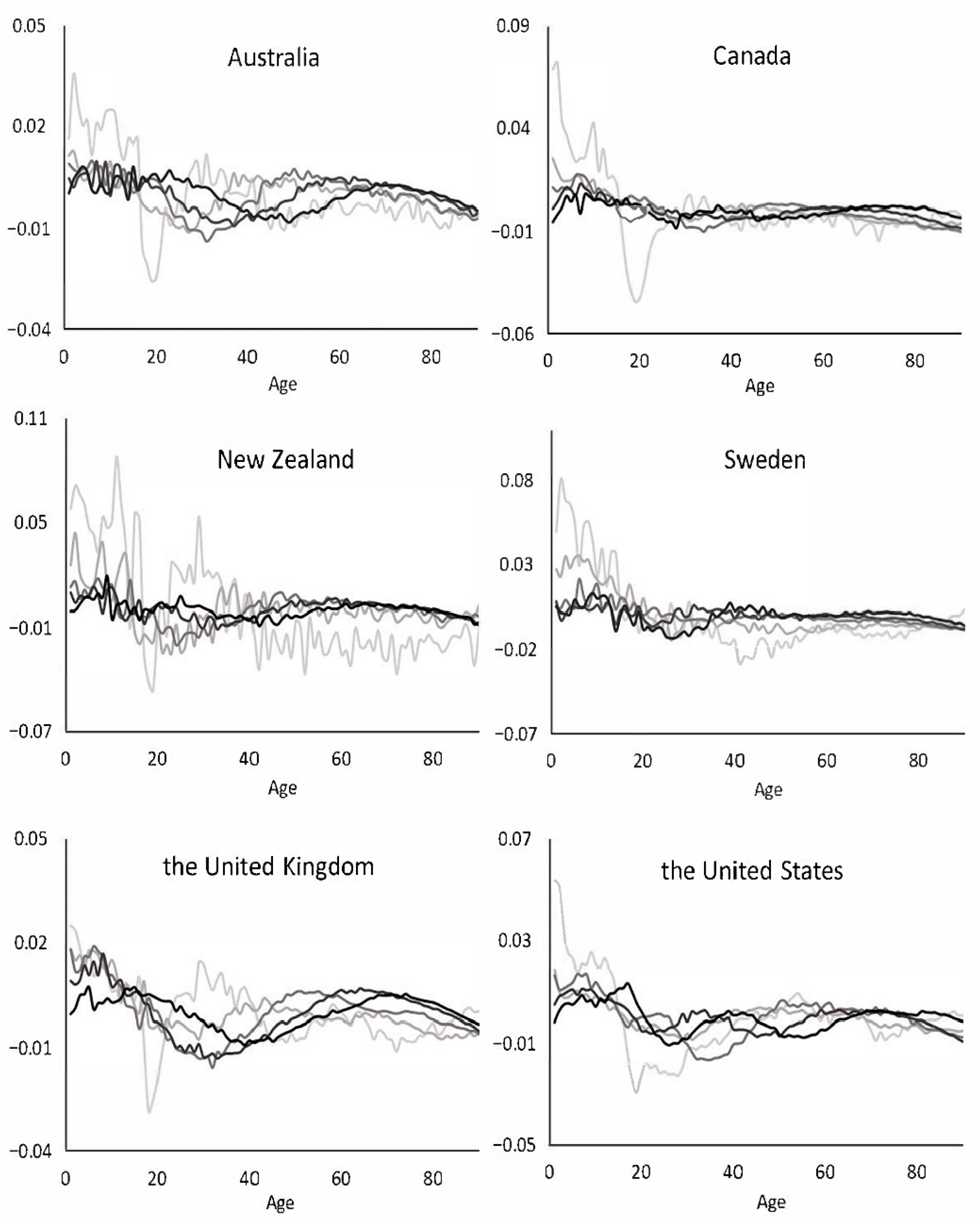
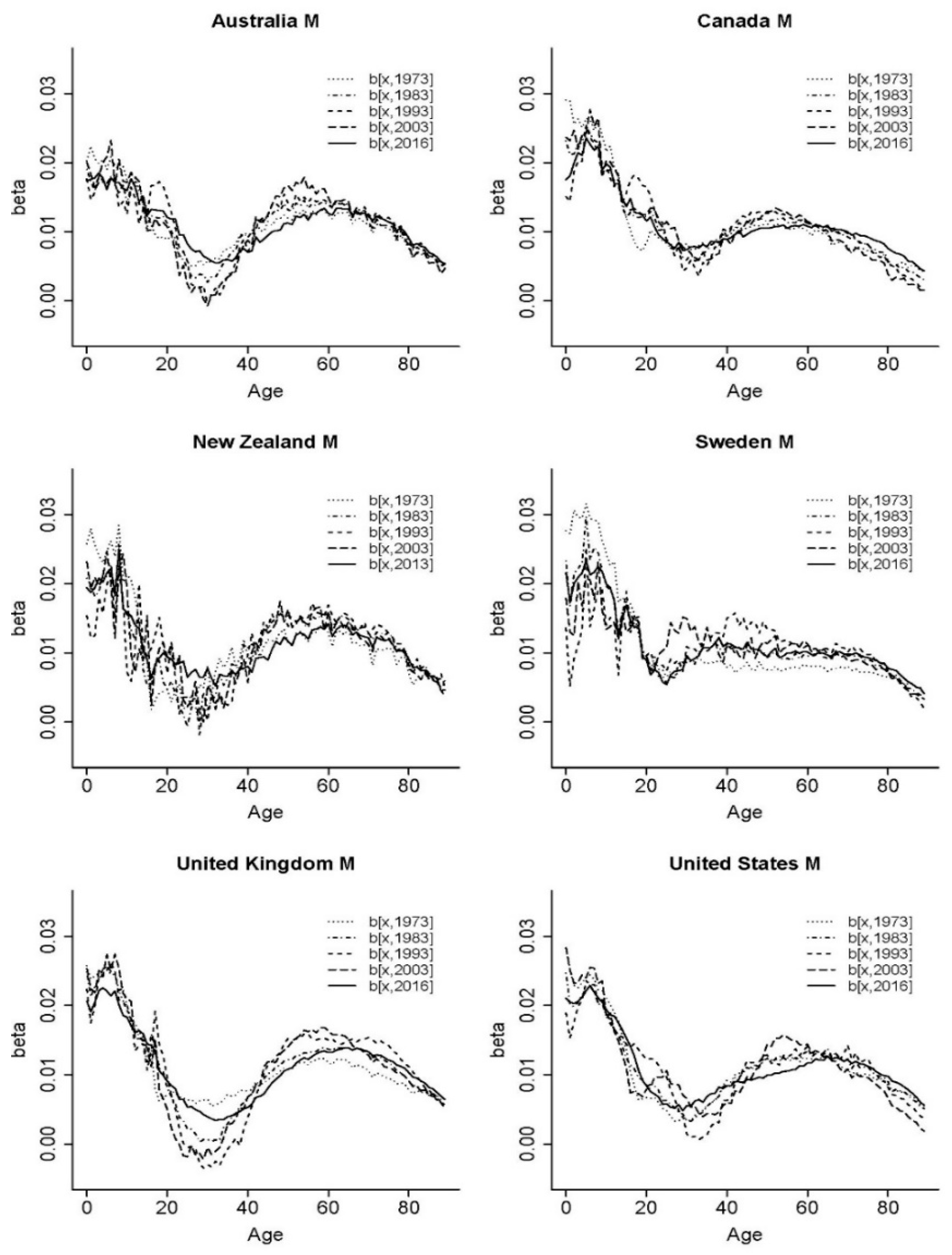
Inspired by the findings in Carter and Prskawetz (2001), we first examined the structure of the age effects under the Lee-Carter model. Setting the same length of fitting periods as in their paper, the first subsample included years 1950–1973. Then, both the starting and ending points of the subsample increased by one year sequentially until the latest data in the sample were employed. For example, the sample period between 1950 and 2016 can be arranged to form 44 subperiods. Figure 1 shows the estimated age sensitivity parameters of the Lee-Carter model calibrated using the sequential subsamples. The colour intensity of the curve increases with the date of the corresponding subsample, with the darkest representing the parameters obtained from the latest subperiod. For presentation purposes, we only displayed the values with a 10-year gap.

It was interesting to see that the age responses were wave-like, and the shape propagated and deformed over time. These observations inspired us to fit a Fourier series with time-varying parameters comprised of single or multiple sine and cosine waves. The Fourier analysis was initially introduced by the mathematician Baron Jean Baptiste Joseph Fourier in his study about temperature distributions. It helped to decompose complicated periodic functions into a sum of sinusoidal components and identify critical features of interest. It can interpret characteristics of a time series process (e.g., peaks, troughs, cycles) in terms of values in the frequency domain (e.g., frequencies, amplitudes, phases). Researchers have applied the Fourier analysis to a wide range of fields such as optics (Lombardet et al. 2005; Mei and Svanberg 2015), agriculture (Canisius et al. 2007), electricity (Amaral et al. 2008), magnetics (Gysen et al. 2010) and insurance (Powers and Powers 2015). For more technical details of Fourier series and its applications, one may refer to Chapters 1 and 2 of Bracewell (1978).

An alternative to the Fourier approach is fitting a smooth curve using cubic splines comprising piecewise third-order polynomials joined at a set of knots. Splines are capable of producing a good fit when the number of knots is sufficiently large. However, the coefficients of splines are not readily interpretable, causing difficulties in choosing an appropriate method to predict their future trends. In this paper, we applied both the Fourier function and cubic splines to capture the development of age patterns of mortality and compare their performances with those under the baseline Lee-Carter model.

Overall, we propose a potential method to model the time-varying age patterns of mortality development. Our main objective was to investigate the performance of the proposed models and to test the impact of incorporating the age effects of structural changes. The remainder of the paper is organized as follows. Section 2 introduces the specifications of the Lee-Carter and proposed models constructed using the Fourier series and cubic splines. Section 3 and Section 4 compare the prediction performance of the mortality models and conduct backtesting using mortality data of the six above-mentioned countries. Section 5 presents a case study to illustrate how the proposed model can readily integrate the age and period effects of structural changes based on data from the United Kingdom. Section 6 concludes.

2. Methodology

The original Lee-Carter model expresses the logarithm of central death rates $\ln \left(m_{x,t}\right)$ as a linear/bilinear combination of age and time effects,

$$\ln \left(m_{x,t}\right)={\alpha }_x+{\beta }_x{k}_t+{ϵ}_{x,t},$$

(1)

where ${\alpha }_x$ represents the average mortality level at each age, $k_t$ is a time-varying mortality index, ${\beta }_x$ is the age-specific factor2 indicating the sensitivity of $\ln \left(m_{x,t}\right)$ to the changes in $k_t$, and ${ϵ}_{x,t}$ follows a Gaussian distribution with a mean of zero. As mentioned earlier, there has been clear evidence against the assumption of a time-invariant age response in the original Lee-Carter model, which can be addressed by allowing the age sensitivity factor to vary over time.

The term ${\beta }_{x,t}$ is denoted as the age response at age x in year $t$. Projecting ${\beta }_{x,t}$ directly brings almost a hundred time series processes for a wide age range. To reduce the dimensionality, a parametric function can be fitted to the time-varying age response. Specifically, we considered two methods—the Fourier-like series and cubic splines with time-varying parameters and refer to them as the Fourier and cubic Lee-Carter models in the rest of the paper. Unlike other approaches of dimensionality reduction such as the principal component analysis that contains artificial variables (Vyas and Kumaranayake 2006), the Fourier series has the advantage that its parameters are interpretable. This property becomes useful in incorporating assumptions of future age patterns into mortality projections.

For a given sample relating to year t, the age response ${\beta }_{x,t}$ can be expressed as a series ordered by age x. We then add the time dimension to the coefficients and apply a Fourier series3 as follows,

$$\begin{gathered} {\beta }_{x,t}=a_{0,t}+{\displaystyle \sum }_{j=1}^N{A}_{j,t}\sin \left(2\pi f_j\times x+P_{j,t}\right)+e_{x,t} \\ =a_{0,t}+{\displaystyle \sum }_{j=1}^N{b}_{1,j,t}\sin \left(2\pi f_j\times x\right)+{\displaystyle \sum }_{j=1}^N{b}_{2,j,t}\cos \left(2\pi f_j\times x\right)+e_{x,t}, \end{gathered}$$

(2)

where $a_{0,t}$ represents the intercept of the Fourier series relating to year t, $N$ is a predefined total number of harmonic waves, the amplitude parameter $A_{j,t}$ measures the distance from the peak (or trough) to the central value, the phase parameter $P_{j,t}$ represents the number of “sinusoidal periods” (measured in the age dimension) that has been shifted from a predefined point, the frequency parameter $f_j$ gives the number of cycles per unit of age, and $e_{x,t}$ is the Gaussian error term with null mean. One could use time-varying frequencies to obtain a better fit, but allowing frequency values to change over time leads to different dimensions of Fourier parameters at different points of time, which makes the extrapolation infeasible. Given the frequency values, one can estimate $a_{0,t}$, $b_{1,j,t}$, and $b_{2,j,t}$ via linear regression sequentially. 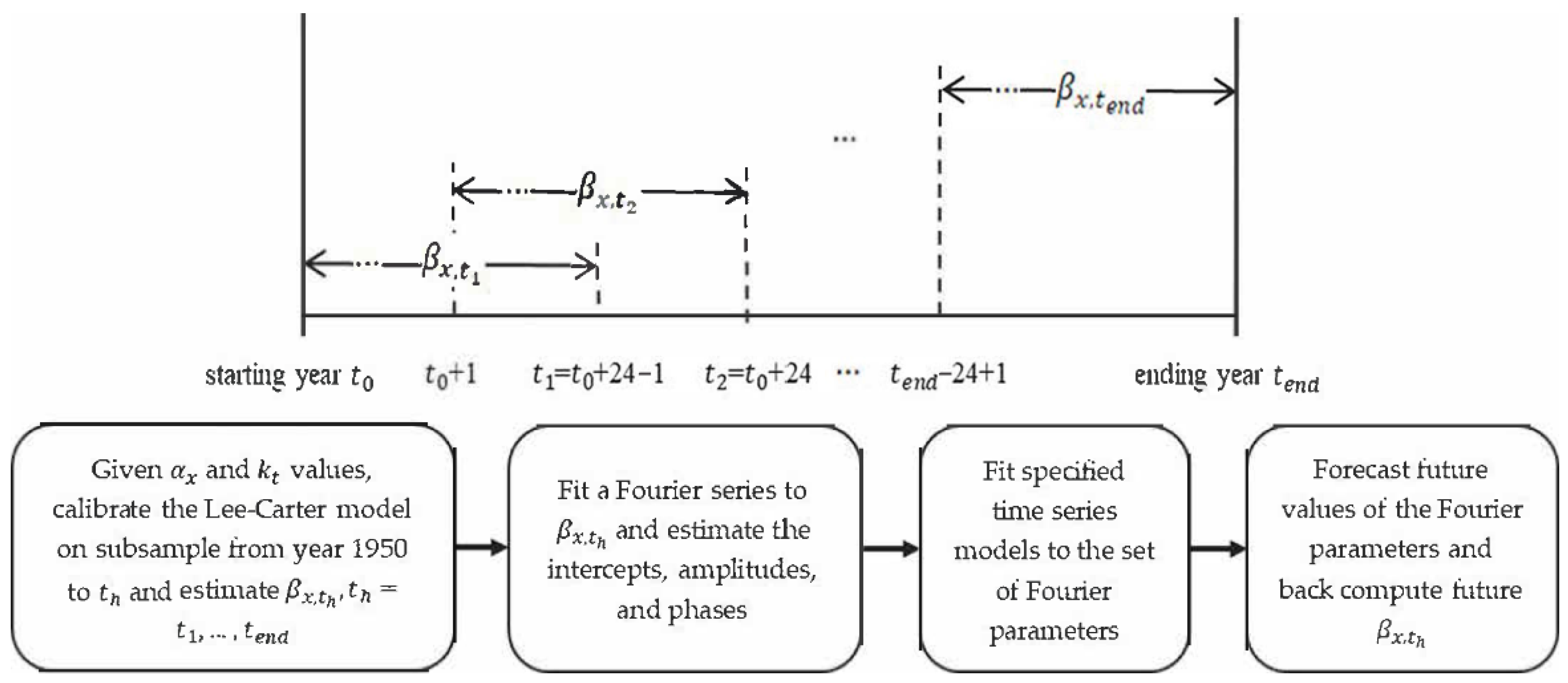Figure 2 presents a flow diagram of the modelling process of ${\beta }_{x,t}$.

As illustrated, the entire sample period can be split into different subperiods. These subperiods were structured as overlapping to some extent4 in order to obtain more data points and smoother changes over time for the Fourier parameters. However, these overlapping subsamples would give different ${\alpha }_x$ and $k_t$ values. To make the estimates of the age sensitivity factor more comparable across the subperiods, we first fitted the Lee-Carter model to the whole sample period and treated the computed ${\alpha }_x$ and $k_t$ as given. The Lee-Carter model was then calibrated to each (overlapping) subperiod in turn using a Poisson updating scheme5 (Brouhns et al. 2002; Li 2013) and a unique set of ${\beta }_{x,t}$ values was obtained, where $t$ referred to the last year of a subsample. For instance, the first ${\beta }_{x,t_1}$ corresponded to the age response over the period from the starting year of the sample to 24 years later; the last one ${\beta }_{x,t_{end}}$ corresponded to the years between the ending year of the sample and 24 years earlier. The age sensitivity parameters calibrated on different subperiods of the sample from 1950 to the latest year are plotted in Figure 3.

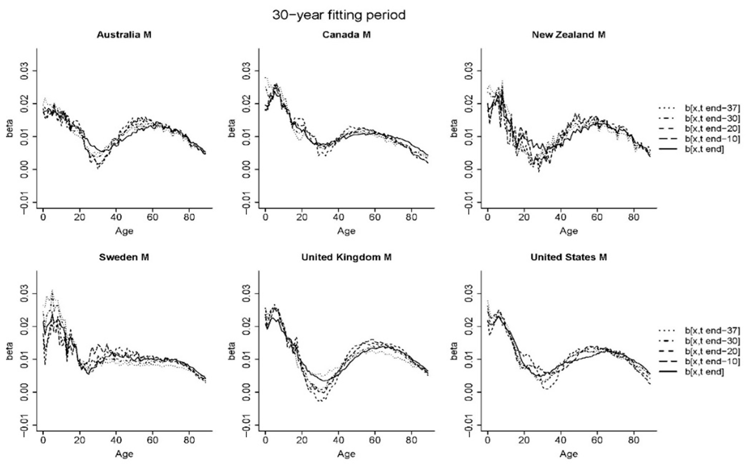
Here, we followed the choice of Carter and Prskawetz (2001) and used an arbitrary fixed value of 24 years for each subsample, although other lengths of subperiods may be chosen. We tested four different lengths of the subperiods and presented the estimated age response parameters in Figure A1 in Appendix A. When longer subperiods were employed, the changes in the shape of age response were relatively less evident. Overall, the lengths of 20, 24, and 30 years produced a similar extent of “volatility” in the age response parameters calibrated on sequential subsamples6. On the other hand, the 10-year window appeared to be too short and the resulting parameter estimates were volatile.

In general, the curves of most of the countries showed two peak values occurring at the youngest ages and around ages 50–65. One exception was Sweden whose age-specific response curve was relatively flat over middle ages. The magnitude of the first peak tended to be greater than the other, implying a high sensitivity of new-borns to mortality changes. Compared with the curves presented in Figure 1, the age sensitivity factors in Figure 3 showed less evident development patterns over time (e.g., peaks shifting towards higher ages). The ${\beta }_{x,t}$ plotted in Figure 3 were estimated by treating the same set of ${\alpha }_x$ and $k_t$ values as given. Therefore, the shapes of ${\beta }_{x,t}$ from different subperiods were more comparable with one another than those estimated using different sets of ${\alpha }_x$ and $k_t$.

When modelling the human age response, it was desirable to keep the main features in the original values such as the peaks mentioned above. Also, the spikes at the youngest ages might have affected the estimates of Fourier parameters which then would not capture the characteristics at older ages7 adequately. To differentiate between the noticeable patterns at younger and older ages, the estimated age sensitivity factors displayed in Figure 3 may be described as one quarter of a complete wave at the younger ages followed by a half wave with a smaller amplitude over the remaining age range. Therefore, we decomposed the age response into two waves and estimated two sets of Fourier parameters instead of modelling it as a whole. For each of the two regions, we employed only one harmonic wave ($N=1$) to depict the shape of age sensitivity factors to avoid over-parameterisation8. The adjusted Fourier series with a split can be expressed as follows,

$$\begin{gathered} {\beta }_{x,t}=a_{0,t}+A_t^{\left(1\right)}\sin \left(2\pi f^{\left(1\right)}\times x+P_t^{\left(1\right)}\right)I\left(x\le x_k\right) \\ +A_t^{\left(2\right)}\sin \left[2\pi f^{\left(2\right)}\times \left(x-x_k\right)+P_t^{\left(2\right)}\right]I(x>x_k)+e_{x,t} \\ =a_{0,t}+\left[b_{1,t}^{\left(1\right)}\sin \left(2\pi f^{\left(1\right)}\times x\right)+b_{2,t}^{\left(1\right)}\cos \left(2\pi f^{\left(1\right)}\times x\right)\right]I\left(x\le x_k\right) \\ +\left[b_{1,t}^{\left(2\right)}\sin \left(2\pi f^{\left(2\right)}\times \left(x-x_k\right)\right)+b_{2,t}^{\left(2\right)}\cos \left(2\pi f^{\left(2\right)}\times \left(x-x_k\right)\right)\right]I\left(x>x_k\right)+e_{x,t}, \end{gathered}$$

(3)

where $a_{0,t}$ is the common intercept shared by the two piecewise functions, $x_k$ is the splitting age at which a wave for the older population starts, $f^{\left(i\right)}$, $A_t^{\left(i\right)}$ and $P_t^{\left(i\right)}$ are the frequency, amplitude and phase parameters of the $i^{th}$ wave, $b_{1,t}^{\left(i\right)}$ and $b_{2,t}^{\left(i\right)}$ are the coefficients of the $i^{th}$ regression, $i=1,2$. The two peak values were observed at age $x_{peak}^{\left(1\right)}$ and $x_{peak}^{\left(2\right)}$, respectively. The frequency values that controlled the lengths of harmonic waves are determined to maintain the observed features of human age sensitivity. As mentioned above, the first wave displayed about one quarter of a complete cycle, suggesting that the length of the wave was approximately $4(x_k-x_{peak}^{\left(1\right)})$. Similarly, the second wave corresponded to a half cycle, so the length of the second wave could be estimated by $2\left(x_{max}-x_k\right)$, where $x_{max}$ was the maximum age in the sample data. Accordingly, the two frequency values $f^{\left(1\right)}=1/[4(x_k-x_{peak}^{\left(1\right)})]$ and $f^{\left(2\right)}=1/\left[2\left(x_{max}-x_k\right)\right]$ were employed. Thereinto, $x_{peak}^{\left(1\right)}$ was chosen as age 0 arbitrarily for all the countries, although the locations of $x_k$ and $x_{peak}^{\left(2\right)}$ were not deduced directly from the graph. They were estimated using the ages at which the minimum and maximum (excluding the first peak) ${\beta }_{x,t}$ were achieved, averaged over all subperiods. Note that $x_{peak}^{\left(2\right)}$ did not affect the choice of frequencies and could have been captured by the second phase parameter. For the six countries considered, the splitting age $x_k$ occurred at around age 30, and the second peak $x_{peak}^{\left(2\right)}$ generally fell within ages 50–60. Specifically, we set $a_{0,t}$ as the age-specific sensitivity value at the linking age which approximated the average level of the first and second waves.

After specifying the frequency values, the amplitude and phase parameters could be estimated via the linear regression method, specifically, for the ith wave, $b_{1,t}^{\left(i\right)}=A_t^{\left(i\right)}\cos \left(P_t^{\left(i\right)}\right),b_{2,t}^{\left(i\right)}=A_t^{\left(i\right)}\sin \left(P_t^{\left(i\right)}\right)$. Rearranging the expressions, we could calculate the $A_t^{\left(i\right)}$ and $P_t^{\left(i\right)}$ as: $A_t^{\left(i\right)}={\left({\left(b_{1,t}^{\left(i\right)}\right)}^2+{\left(b_{2,t}^{\left(i\right)}\right)}^2\right)}^{1/2}$ and $P_t^{\left(i\right)}=arctan\left(b_{2,t}^{\left(i\right)}/b_{1,t}^{\left(i\right)}\right)$.

However, the identification problem existed in estimating the phase parameter due to the periodicity of trigonometric functions. For instance, $arc tan\left(0\right)$ could be either 0 or $\pi$, as $P_0$ and $P_0+\pi$ always resulted in equivalent tangent values. Therefore, we imposed restrictions on the range of the two phase parameters according to the general shape of age sensitivity factors. Since one would have expected a peak followed by a decreasing pattern at young ages, the range of $P_t^{\left(1\right)}$ was set to ($\pi /4,5\pi /4$). Similarly, the range of $P_t^{\left(2\right)}$ was restricted to (−$\pi /2,\pi /2$), so that a bell-shaped curve could be observed for ages after the knot $x_k$. Next, we explained the rationale of these two constraints.

Several features can be preserved when fitting a Fourier series to the age sensitivity factor based on the historical shape. On the one hand, the curve went downward before the splitting age, although such a pattern is not necessarily monotonic from age 0. On the other hand, the age response at ages older than the knot $x_k$ generally showed a bell shape for the six countries considered. Based on these observations, Figure 4 illustrated possible shapes of $\sin \left(x+P_t^{\left(i\right)}\right)$ over the domain $x\in \left(0,\pi /2\right)$ and $x\in \left(0,3\pi /2\right)$ for $i=1 \mathrm{and} 2$, respectively. Since the two frequency parameters were determined such that the first (second) wave corresponded to a quarter (half) of a complete wave, we focused on the curves for $x<\pi /2$ ($x<\pi$) on the left (right) graph. As shown in the left column of Figure 4, when the first phase parameter $P_t^{\left(1\right)}$ took values between $\pi /4$ (red curve) and $5\pi /4$ (green curve), the first quarter of the waves were mainly downward, matching with the historical characteristics of ${\beta }_{x,t}$ at younger ages. For possible shapes of ${\beta }_{x,t}$ at older ages (right column), the first half of the waves $\sin \left(x+P_t^{\left(2\right)}\right)$ demonstrated a bell shape when $P_t^{\left(2\right)}$ ranged from $-\pi /2$ to $\pi /2$.

Overall, for each t we fitted the Fourier series with two waves to ${\beta }_{x,t}$ and estimated the Fourier parameters $a_{0,t}$, $A_t^{\left(i\right)}$ and $P_t^{\left(i\right)}$, $i=1,2$. Accordingly, the dimension was reduced from 90 (ages) to 5 (one intercept, two amplitude, and two phase parameters). The intercepts, amplitudes and phases were time-varying, the future values of which were predicted via time series models. Forecasts of the age response could then be computed from the predictions of its Fourier parameters.

The above specification of the Fourier Lee-Carter model is similar to the cubic spline technique which has been widely applied in smoothing mortality rates (e.g., Currie et al. 2004; Armstrong 2006; De Jong and Tickle 2006; Debón et al. 2006). A function $f\left(x\right)$ defined on $\left[a,b\right]$ with $m$ interior knots ${\xi }_i \left(i=1,2,\dots ,m\right)$ is a cubic spline if it is a cubic polynomial in each of the intervals and $f\left(x\right)$ is continuous up to the second derivative. Thereinto, one sub-category that solves the potential problem of erratic fitting at boundary values is referred to as natural cubic splines. It imposes additional constraints on the second and third derivatives at the two limits $a$ and $b$ such that $f\left(x\right)$ is linear in the two boundary intervals $\left[a,{\xi }_1\right]$ and $\left[{\xi }_m,b\right]$. We borrowed this concept and considered a so-called cubic Lee-Carter model whose age sensitivity factor ${\beta }_{x,t}$ was modelled as natural cubic splines. The idea was to interpolate a curve using segments of cubic polynomials connected by knots that were placed at turning points. As analyzed above, there were two peaks at ages $x_{peak}^{\left(1\right)}$ and $x_{peak}^{\left(2\right)}$ and one trough at age $x_k$. The three internal knots were selected for our cubic Lee-Carter model and located at (0, $x_k$, $x_{peak}^{\left(2\right)}$). The chosen knots would result in a decreasing trend from age 0 to the trough age $x_k$, followed by a bell-shaped curve peaked at $x_{peak}^{\left(2\right)}$. The piecewise polynomial could be estimated using linear regression and the R package “splines”. Again, we modeled the cubic-spline parameters as time series processes to predict future age sensitivity. In matrix notation, the age sensitivity factor under the cubic Lee-Carter model could be written as follows,

$${\mathsf{\beta }}_t=H_t{c}_t+e_t,$$

(4)

where the $\left(x_{max}\times 1\right)$ vector ${\mathsf{\beta }}_t={\left({\beta }_{0,t},{\beta }_{1,t},\dots ,{\beta }_{x_{max},t}\right)}^{\prime }$ referred to the age response at all ages at time $t$, vector $e_t$ comprised the constants and error terms for each regression of ${\beta }_{x,t}$. $H_t$ was the ($x_{max}\times 4$) basis matrix defining the vector space of the spline function, which could be obtained by the command “ns” in R. Then the $\left(4\times 1\right)$ vector $c_t={\left(c_{1,t},c_{2,t},c_{3,t},c_{4,t}\right)}^{\prime }$ containing the time-varying cubic-spline coefficients was estimated via linear regression.

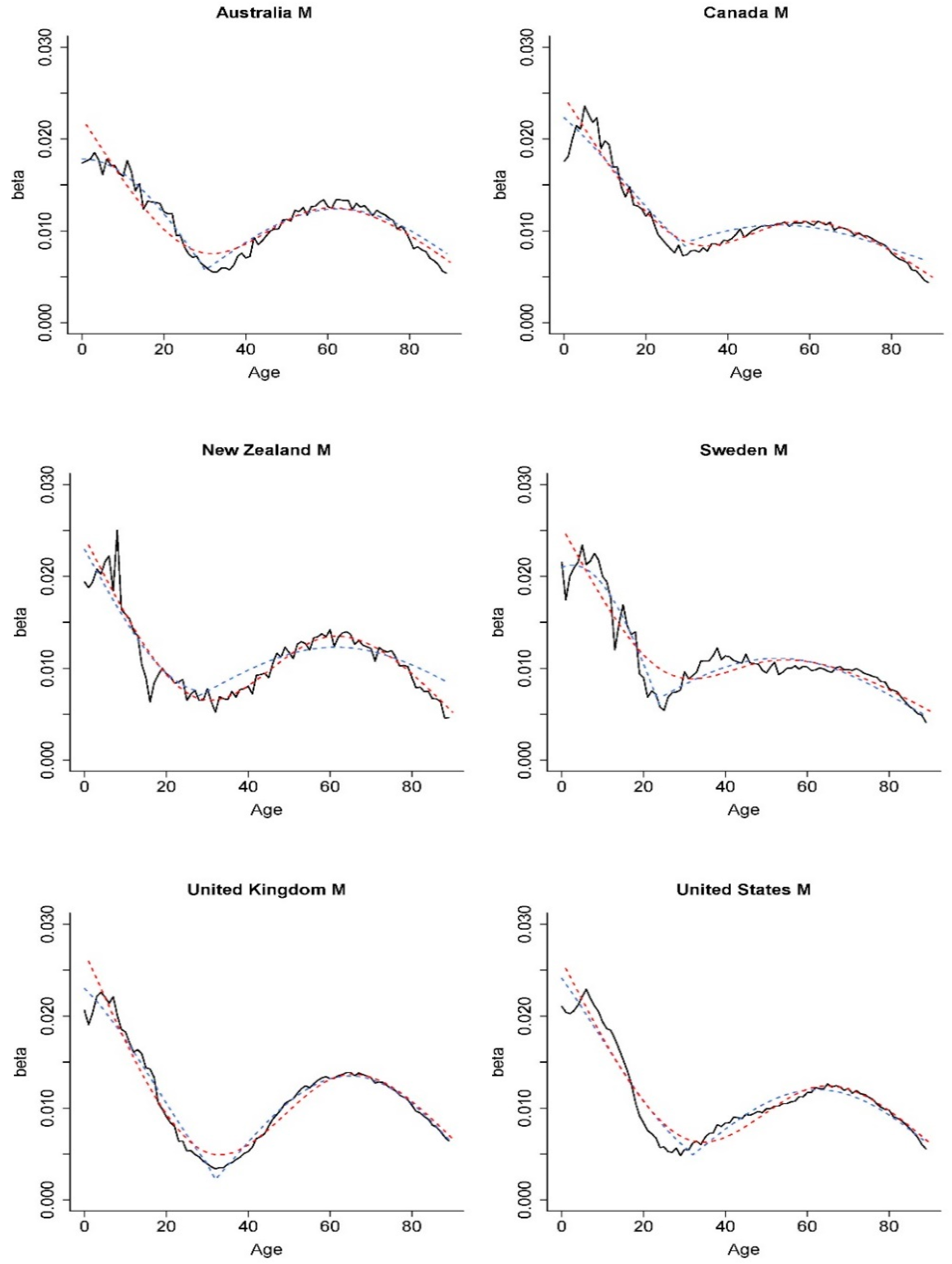
Figure 5 displays the estimated and fitted values of the age sensitivity parameter using the Fourier and cubic-spline approaches based on the mortality data of the latest 24-year subperiod. Both methods can capture the general shape of the age response. Unlike the Fourier approach, however, no meaningful interpretation was available for the coefficients of the cubic splines.

The primary purpose of introducing a time-varying age sensitivity parameter is to discover whether the age effects of structural changes in mortality can be modelled and predicted over time. We now examine and compare performances of the original Lee-Carter model, Fourier Lee-Carter model and cubic Lee-Carter model in the following sections.

3. Projections

We could now use the specified model to produce projections of future mortality rates. The original Lee-Carter model is calibrated on the entire sample period to estimate the age-specific parameter ${\alpha }_x$ and the mortality index $k_t$. These two parameters were then treated as given to find the values of a set of age sensitivity factors and their corresponding Fourier and cubic-spline parameter estimates. Future mortality scenarios under the Fourier model and cubic model were generated by forecasting the time-varying parameters and the mortality index.

Since the shape of the fitted Fourier functions is controlled by interpretable Fourier parameters, their time series choices are made to project the age effects that are in accordance with the past patterns. As illustrated in Figure 3, which plots the estimated age responses from different subperiods, the waves after the splitting age have been shifting over time, although the extent of movements has not been as evident at younger ages. Accordingly, we modelled the intercepts, amplitudes, the first phase parameter, and the first difference of the second phase parameter as stationary autoregressive processes with order 1 (AR(1)). Such specification implied that the height (the vertical distance from peak to trough) of ${\beta }_{x,t}$ would converge to a constant, and the second wave would shift over time9. As noted above, the cubic-spline parameters did not have meaningful interpretations, and it was not quite straightforward to select appropriate time series models. Thus, we modelled them by stationary AR(1) processes to obtain a convergent age response. The mortality index was fitted with an RWD. In a case where the estimated AR(1) model was not stationary, we replaced it with a random walk (RW) without drift. These time series models were adopted for the rest of the paper.

Figure 6 illustrates the predicted life expectancy10 at birth ($e_0$) under the original Lee-Carter model and the two variations proposed here. We can see from these plots that allowing for a time-varying age sensitivity factor generally results in higher projections for all six datasets. The Fourier assumption tended to predict the highest life expectancy at birth (about 1 year greater than that under the Lee-Carter baseline model in 2050) among the three candidates based on the male mortality data of Canada, New Zealand and Sweden, though the cubic Lee-Carter model did not show much difference from the baseline results for New Zealand. For Australia, the United Kingdom and United States, the two modelling methods of the age response showed little difference in their forecast life expectancy values: the curves produced under the cubic approach were only marginally higher (lower) than that under the Fourier approach for Australia and the United Kingdom (the United States). Besides, the two proposed models generated predictions higher than those under the original Lee-Carter model, though to a lesser extent than for Canada, New Zealand and Sweden under the Fourier approach. Next, we compared the forecast accuracy of the three models via out-of-sample testing on a rolling-window basis.

4. Backtesting

4.1. Rolling-Window Backtesting

The primary objective of the newly proposed models was to capture features of the evolution of the age response over time. We could examine the forecasting performance of the Fourier and cubic Lee-Carter models against the observed data via backtesting (also known as out-of-sample testing). The original Lee-Carter model was selected as the baseline model for comparison purposes. The entire sample was split into two periods, where the first (in-sample) part was used for fitting, and the second (out-of-sample) part was used to examine the predictive power of the mortality models. The forecast accuracy was assessed by the mean absolute percentage error (MAPE) of predicted log central death rates and period life expectancies. It was calculated as $\mathrm{MAPE}=\frac{1}{n_d}{{\displaystyle \sum }}_{x,t}\left|\frac{O_{x,t}-F_{x,t}}{O_{x,t}}\right|$, where $n_d$ was the number of data points, and $O_{x,t}$ ($F_{x,t})$ was the observed (forecasted) value of the measure under consideration. However, the results of usual backtesting could have been sensitive to the sample split. Therefore, we conducted the backtesting on a rolling-window basis. The first in-sample period was from 1950 to 1989 (the first 40 years), and the remaining 27 years (from 1990 to 2016) constituted the corresponding out-of-sample period. Then we fitted the mortality models using the first 41 years of data and ed them over the next 26 years, and so on until the prediction period reduced to 5 years. The averaged MAPE value of the 23 splits was calculated to compare the overall performance of the three models.

The backtesting results for the six countries are given in

Table 1. MAPE values (%) of projected log central death rates of all ages and 30-year age groups (rolling-window basis). The minimum MAPE values for each age group and each country are given in bold.

Age Group	Overall			0–29			30–59			60–89
Population	LC	Fourier	Cubic	LC	Fourier	Cubic	LC	Fourier	Cubic	LC	Fourier	Cubic
Australia	3.02	2.92	2.88	3.23	3.34	3.24	1.82	1.74	1.70	4.01	3.67	3.70
Canada	2.66	2.31	2.53	2.54	2.33	2.31	1.39	1.36	1.32	4.05	3.23	3.95
New Zealand	4.50	4.36	4.35	5.21	5.29	5.17	2.98	2.95	2.91	5.31	4.85	4.97
Sweden	3.64	3.29	3.52	4.38	4.67	4.30	2.96	2.80	2.86	3.58	2.40	3.39
United Kingdom	2.71	2.51	2.57	2.25	2.25	2.21	1.26	1.23	1.13	4.62	4.06	4.38
United States	2.03	1.92	1.96	1.59	1.62	1.58	1.58	1.64	1.49	2.93	2.48	2.80

, which displays the MAPEs of projected log central death rates for different age groups. Columns named ‘LC’, ‘Fourier’ and ‘Cubic’ refer to results generated from the original Lee-Carter model, Fourier Lee-Carter model and cubic Lee-Carter model, respectively. Considering the entire age interval, the two newly proposed mortality models outperformed the original Lee-Carter model in all cases. Specifically, the Fourier approach beat the others when Canadian, Swedish, British and American data were considered, although the cubic-spline method was preferred for Australia and New Zealand. The most significant improvements were observed under the Fourier Lee-Carter model for Canada and Sweden, with a reduction of 0.35% or more in MAPE value. The extent of reductions from adopting a time-varying age response was satisfactory, considering that the baseline errors were mostly between 2–3%.

When examining 30-year age groups, the two newly proposed models still produced more accurate projections than the original Lee-Carter model, except for the youngest age group in Australia. The best choice among the three candidates and the significance of improvements in forecast accuracy demonstrated some variations across age groups. In more detail, the cubic Lee-Carter model gave the lowest MAPE value for five out of the six countries over ages 30–59, and the Fourier approach was preferred for older populations in all of the six countries. In addition, the improvements from assuming a time-varying age response for the oldest age group were generally more notable than those for the other two age ranges. In the case where the Fourier Lee-Carter model was the optimal choice over all ages, the main contribution came from the accurate forecasts for the age range 60–89. For instance, under the Fourier assumption, the MAPEs for the elderly in Canada and Sweden decreased respectively by 0.82% and 1.17%, although these numbers under the cubic-spline assumption were only 0.10% and 0.19%. On the other hand, the prediction errors in the two countries between the two methods were more or less the same over ages 0–29 and 30–59. So, the overall performance of the Fourier Lee-Carter model was mainly driven by the improvements for the oldest population. All these results suggested that the age sensitivity parameter in the Lee-Carter model did not remain the same over time, and an allowance for the evolution at different ages could improve the forecasting performance. In particular, the oldest age group had experienced more noticeable changes than the other two. The outperformance under the Fourier Lee-Carter model was largely attributable to the nonstationary time series choice of the second phase parameter. Following historical patterns, the second peak age $x_{peak}^{\left(2\right)}$ of the projected age sensitivity tended to move towards higher ages over time, leading to higher sensitivity for those aged 60–89. Although the cubic parameters were also time-varying, it was not clear what time series choices would lead to faster mortality reductions at higher ages. Since they were predicted by stationary AR(1) models that converged quickly, the evolution of age patterns was less evident. Given the same changes in the mortality index, the Fourier model suggested faster mortality improvements for the elderly than the other two models, which was more in line with historical data.

As an additional measure of forecast accuracy, we also presented the MAPE values of projected life expectancies at ages 0 ($e_0$) and 60 ($e_{60}$) under the original Lee-Carter model, the Fourier Lee-Carter model and the cubic Lee-Carter model in

Table 2. MAPE values (%) of projected life expectancies at ages 0 and 60 (rolling-window basis). The minimum MAPE values for each age and each country are given in bold.

Age Group	${\mathit{e}}_0$			${\mathit{e}}_{60}$
Population	LC	Fourier	Cubic	LC	Fourier	Cubic
Australia	1.31	1.22	1.19	4.16	3.72	3.78
Canada	1.17	0.87	1.10	4.42	3.14	4.15
New Zealand	1.78	1.64	1.64	4.90	4.23	4.43
Sweden	1.30	0.90	1.18	3.98	2.07	3.67
United Kingdom	1.46	1.31	1.34	5.35	4.59	4.86
United States	0.87	0.83	0.82	3.08	2.45	2.81

. Similar to the observations on the log central death rates, incorporating time-varying age patterns in the Lee-Carter model tends to predict future life expectancies more accurately for the six countries. The prediction errors of life expectancies at ages 0 and 60 under the Fourier (cubic) Lee-Carter model decreased by about 0.1–0.4% (around 0.1%) and 0.5–1.9% (0.3–0.5%), respectively. Again, the assumption of Fourier age patterns tended to work well at higher ages. In fact, the results of all datasets suggested that the Fourier age sensitivity factor brought the most noticeable reductions in forecast error for the higher-age life expectancy. In particular, the forecast accuracy of life expectancy at age 60 improved by over 0.7% for the male populations in three countries—Canada, Sweden and the United Kingdom. Although the Fourier Lee-Carter model tended to outperform the original Lee-Carter model for both measures, applying cubic-spline assumptions on the patterns of the age response also generated some good performances. For life expectancy at birth, the Fourier Lee-Carter model had the best fit to the male mortality data of Canada, New Zealand, Sweden and the United Kingdom, although the cubic-spline assumption was preferred for Australia and the United States. However, we emphasize that the difference in prediction errors between the two proposed approaches was less than 0.1% when the cubic-spline method was optimal. In the other cases, the Fourier assumption tended to beat its rival more evidently.

Overall, the forecast accuracy of log central death rates and life expectancies coulkd be improved when the age sensitivity parameter in the Lee-Carter model is modelled with the Fourier series or cubic splines. Nevertheless, the extent of outperformance of the two models may vary over different age groups. Our results indicated that the Fourier (cubic) Lee-Carter model might be preferred for older (middle) age ranges, and that the Fourier tended to outperform the cubic when the entire population was considered. Next, we incorporated error terms into our projection results and examined the three mortality models regarding their ability to capture potential structural changes.

4.2. Backtesting with Simulation

To further evaluate the predictive power of the proposed mortality models, we used the Monte Carlo simulation to calculate the 95% prediction intervals for life expectancies at key ages. The length of the forecasting (out-of-sample) period was set to 15 years, and the previous years of data were employed as the fitting (in-sample) period. The proportions of historical life expectancy values not captured by the 95% prediction intervals are displayed in

Table 3. Proportions (%) of observed life expectancies at ages 0 and 60 falling outside 95% prediction intervals, predicted over the last 15 years of the sample.

Age Group	${\mathit{e}}_0$			${\mathit{e}}_{60}$
Population	LC	Fourier	Cubic	LC	Fourier	Cubic
Australia	0	0	0	60	20	20
Canada	73	47	73	87	87	87
New Zealand	17	0	0	75	0	50
Sweden	53	0	13	67	0	60
United Kingdom	40	13	20	87	53	67
United States	7	0	0	87	67	87

. It is shown that the proportion of outliers of life expectancy at birth (age 60) under the baseline model ranged from around 0% to 70% (60% to 90%) for the six datasets. Under the Fourier and cubic-spline assumptions, this proportion reduced by up to around 70%, the degree of which varied by country. For instance, when the Fourier age sensitivity factor was adopted, the observed life expectancy values at both ages moved well within the prediction intervals for New Zealand and Sweden. Generally, the outliers of life expectancy at birth were fewer than those at age 60. Overall, the two proposed methods offered significant improvement in performance over the baseline model for most of the six datasets, confirming the presence of time-varying age patterns.

Figure 7 displays the historical and predicted life expectancies at birth and age 60 for Australia and Sweden. The 95% prediction intervals generated from the original Lee-Carter model (blue), Fourier Lee-Carter model (red) and cubic Lee-Carter model (grey) are plotted on the same graph. The baseline model has the narrowest prediction intervals, followed by the cubic Lee-Carter model and Fourier Lee-Carter model. This is in alignment with our expectation since the original Lee-Carter model only considered the error term in the mortality index, and the two proposed models also involved the error terms from the time-varying age sensitivity. Besides the fundamental differences between the Fourier and cubic-spline assumptions, the distinctions between the two newly proposed methods also came from the time series processes employed. To make the predicted age patterns conform with the observed developments, the second phase parameter in the Fourier Lee-Carter model was fitted by a non-stationary process with increasing uncertainty over time. On the other hand, no meaningful interpretations could be drawn from the coefficients of cubic splines, so all the time-varying parameters of age response in the cubic Lee-Carter model were fitted by stationary AR(1) with bounded variability. In line with the results in Table 3, Swedish life expectancies at ages 0 and 60 were well captured by the prediction intervals from the Fourier Lee-Carter model (red dashed lines). Moreover, Australian life expectancy at birth did not fall outside of the 95% bounds under all the three candidates. Nonetheless, the two proposed approaches had a tendency to result in closer projections (red and grey dotted lines) to the observed values than the baseline model. The Fourier and cubic projections were very close for Australia, although the former performed better for Sweden. For Sweden, the predictions (red dotted lines) under the Fourier Lee-Carter model were quite close to the realized values but this was not the case for the other two methods.

Theoretically, the percentage of values falling outside the 95% prediction intervals was 5%, but even with time-varying age patterns, the outliers of $e_0$ in Canada and the United Kingdom were still greater than 5%. When considering mortality at higher ages, only the results of New Zealand and Sweden under the Fourier Lee-Carter model satisfied this condition. The underlying reason may have been that the proposed models only took into account the time-varying age patterns of structural changes but not the period effects. In the subsequent section, we demonstrate through a case study that our newly proposed models could readily incorporate these two sources of structural changes simultaneously, addressing this issue.

5. Integrating the Age and Period Effects of Structural Changes

In this section, we examined the impact of incorporating the age and period effects of structural changes, either separately or simultaneously. Under the original Lee-Carter model, structural changes are often analyzed in the literature through the period effects. One needs to determine the dates of structural changes (breakpoints in the mortality index), then apply extended models such as the regime-switching model, broken-trend stationary model (time series process with piecewise-linear deterministic trends) and difference stationary model with breakpoints. Coelho and Nunes (2011) argued that the regime-switching model might not be appropriate because mortality reductions caused by medical advancement and healthcare improvements are unlikely to be reversed. They fitted the Lee-Carter model to each gender of eighteen populations with the mortality index modelled by a trend or difference stationary time series process and concluded that a difference stationary model was more suitable in the event of structural shifts. The main purpose of this section is to illustrate that the Lee-Carter model with time-varying age patterns can integrate both the age and period effects of structural changes. The impact of incorporating the period effects of structural changes is explored using the difference stationary model with one breakpoint in this paper11. For demonstration purposes, we present our analysis based on male mortality data from the United Kingdom with the same fitting (1950–2001) and testing (2002–2016) periods as above.

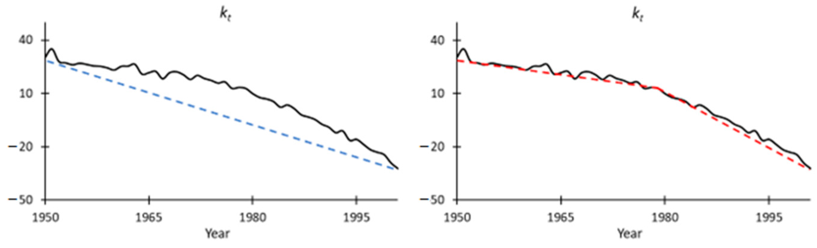
Without considering potential breakpoints, the mortality index $k_t$ can be modelled by a random walk with drift (RWD) as follows:

$$k_t=k_{t-1}+\mu +{\omega }_t,$$

(5)

where $\mu$ is the drift term, and ${\omega }_t$ is the Gaussian error term with zero mean. The drift term is estimated by

$$\widehat{\mu }=\frac{k_{periodend}-k_{periodstart}}{periodend-periodstart},$$

(6)

which only depends on the starting and ending values of $k_t$ over the fitting period. However, as shown by the dashed lines in Figure 8, the slope of the estimated mortality index actually became steeper since the middle of the fitting period. The estimate of the drift term over the whole period would then be too small to capture the future declining trend and underestimate future mortality improvements. In this case, a piecewise RWD might provide a better fit than a straight line (van Berkum et al. 2013). The formula is expressed as follows:

$$k_t=k_{t-1}+{\mu }_i+{\omega }_t,$$

(7)

where ${\mu }_i=\{\begin{array}{c}{\mu }_1, t<t_{bp}\\ {\mu }_2, t\ge t_{bp}\end{array}$, $t_{bp}$ is the date of the detected structural shift. Given the location of the breakpoint, we fit two RWD processes to the calibrated $k_t$ values before and after the break date. Then the latter set of parameter estimates were employed to project future mortality scenarios. We used the R package ‘strucchange’ to identify the potential structural change for male mortality in the United Kingdom between 1950 and 2001. The structural change is detected in 1979, which is in accordance with the graphical observation. For more details of this modelling strategy, one may refer to Section 3 of van Berkum et al. (2013) who investigated the period effects under various mortality models. The estimated value of $\widehat{\mu }$ based on the whole fitting period is −1.35, and the ${\widehat{\mu }}_2$ calculated using the latest period is −2.25.

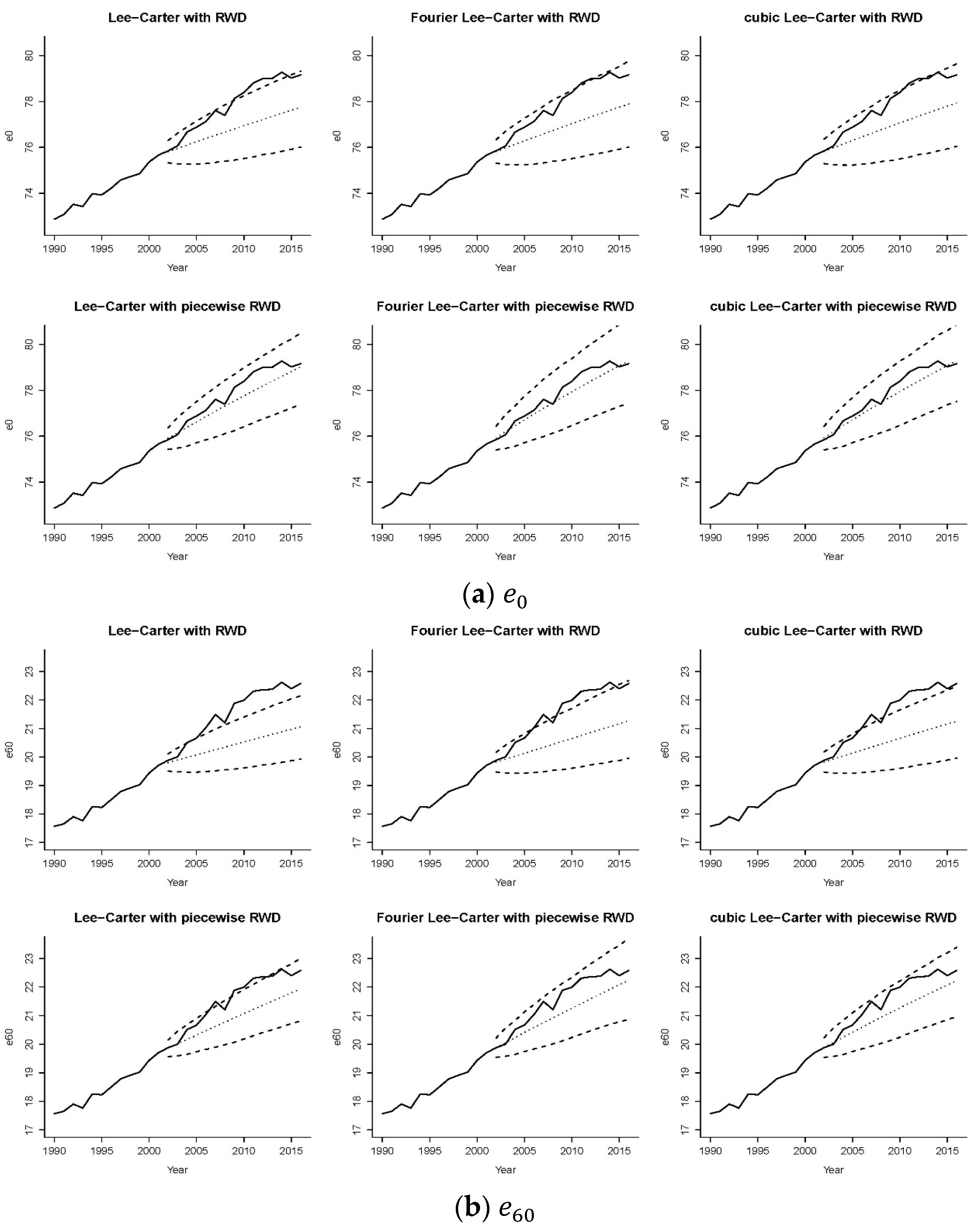
In addition to the inclusion of a breakpoint, we applied the Fourier and cubic Lee-Carter models to incorporate time-varying age patterns. Then we followed the same strategies described in Section 4.2 to simulate future mortality scenarios over the testing period 2002–2016. We compared six sets of mortality forecasts simulated from (1) the Lee-Carter model with RWD, (2) the Fourier Lee-Carter model with RWD, (3) the cubic Lee-Carter model with RWD, (4) the Lee-Carter model with piecewise RWD, (5) the Fourier Lee-Carter model with piecewise RWD and (6) the cubic Lee-Carter model with piecewise RWD. The observed and projected life expectancies at birth and age 60 with 95% prediction intervals are displayed in Figure 9.

There are some interesting observations to make on these diagrams. Comparing the graphs in each row, allowing for time-varying age effects with a Fourier pattern (middle column) tended to give the widest prediction intervals because the model had increasing uncertainty over time on both the mortality index and phase parameters. The projected life expectancy values under the original Lee-Carter model with RWD (the top left graph) showed an apparent deviation from historical data. The gap can be narrowed slightly by introducing a time-varying age effect. Comparing the graphs in each column, we saw that employing piecewise random walk processes could redirect the RWD projection to the ‘right’ trend, with the bottommost panels showing more accurate predictions of life expectancies at both ages 0 and 60 regarding the projected values and prediction intervals when the period effects of structural changes were incorporated. Considering the age effects (the top middle and top right figures) or time effects (the bottom left figure) of structural changes alone yielded better performance than the original Lee-Carter model (the top left figure) did. Furthermore, the integration of the two sources of structural changes (the bottom middle and bottom right figures) produced the best performance among these six models. The above observations held for life expectancies at both ages, although the age effects of structural changes appear to be more influential for older ages. Although employing a piecewise RWD was enough to properly predict $e_0$ of British males (the bottom left graph of Figure 9a), it failed to do so for $e_{60}$. As illustrated by the bottom panel of Figure 9b, the prediction intervals could capture the realized trend of $e_{60}$ only when both the age and period effects of structural changes were taken into account.

The proportions of observed life expectancies at ages 0 and 60 falling outside the prediction intervals under models (4)–(6) for the six countries are displayed in

Table 4. Proportions (%) of observed life expectancies at ages 0 and 60 falling outside 95% prediction intervals, predicted over the last 15 years of the sample. The mortality index is modelled by a piecewise RWD with one breakpoint.

Age Group	${\mathit{e}}_0$			${\mathit{e}}_{60}$
Population	LC	Fourier	Cubic	LC	Fourier	Cubic
Australia	0	0	0	0	0	0
Canada	20	0	7	87	27	87
New Zealand	0	0	0	0	0	0
Sweden	0	0	0	0	0	0
United Kingdom	0	0	0	33	0	0
United States	0	0	0	80	13	40

. Comparing with the figures in Table 3, incorporating the period effects of structural changes reduced the outliers of life expectancies at both ages by up to 75% and up to 67% under the Lee-Carter model with and without time-varying age patterns, respectively. One exception was the Canadian male life expectancy at age 60 under the original Lee-Carter model and the cubic Lee-Carter model whose forecasting errors reduced by 0%. The current results were mostly acceptable under the Fourier Lee-Carter model, especially for life expectancy at birth. With the integration of the two sources of structural changes, significant outliers of $e_{60}$ were still observed in two out of the six cases. Among the two proposed approaches, the Fourier assumption generated better prediction intervals for $e_{60}$, with an improvement over the baseline model of 60% and 67% for Canada and the United States, respectively. This outperformance of the Fourier Lee-Carter model with piecewise RWD was possibly attributable to the unbounded variability assumed for the second phase parameter that was related to the age response at higher ages. Although one may adopt similar time series processes for the cubic-spline parameters, there is no practical interpretation of the cubic-spline coefficients and the choice of time series was hard to justify.

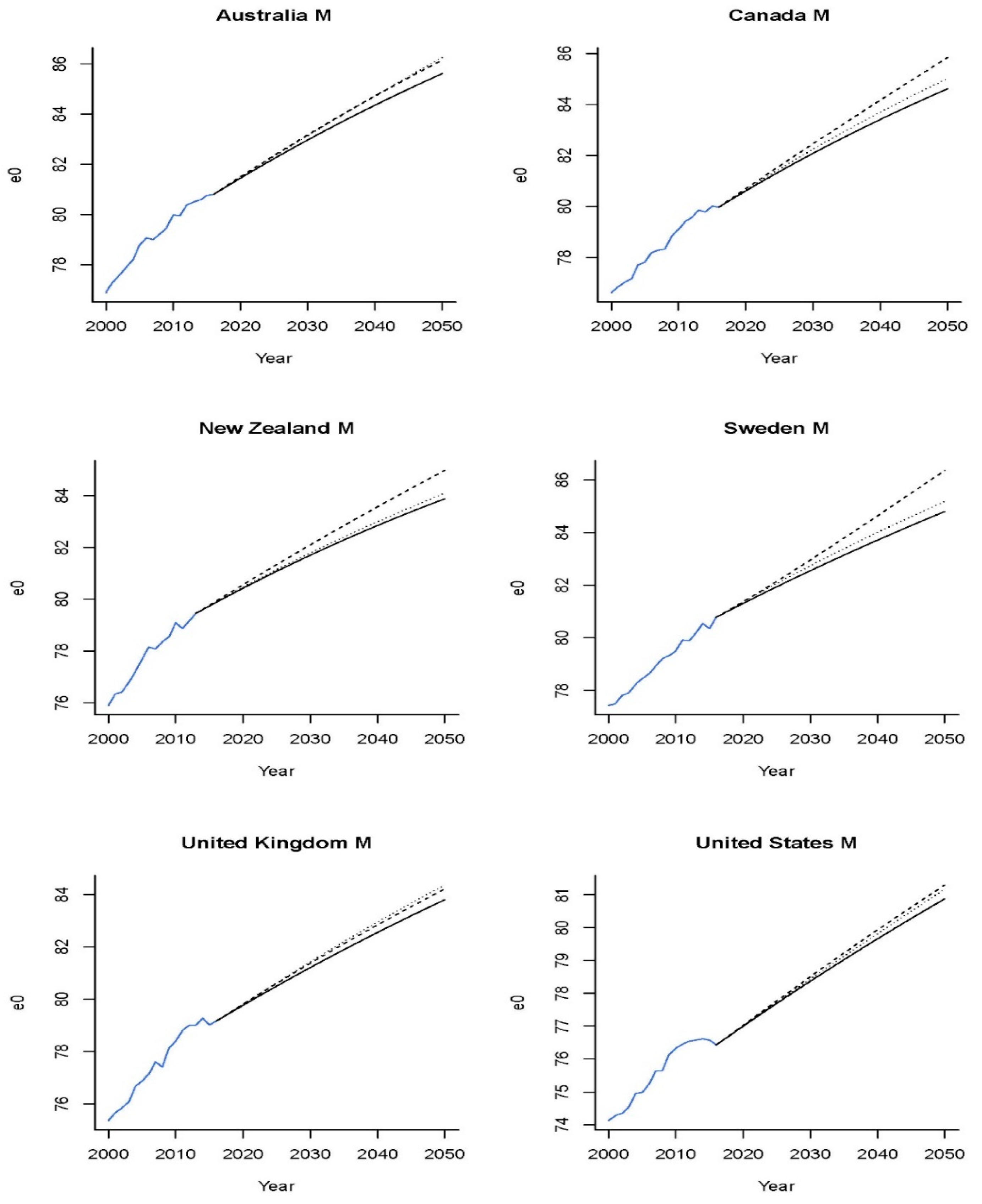
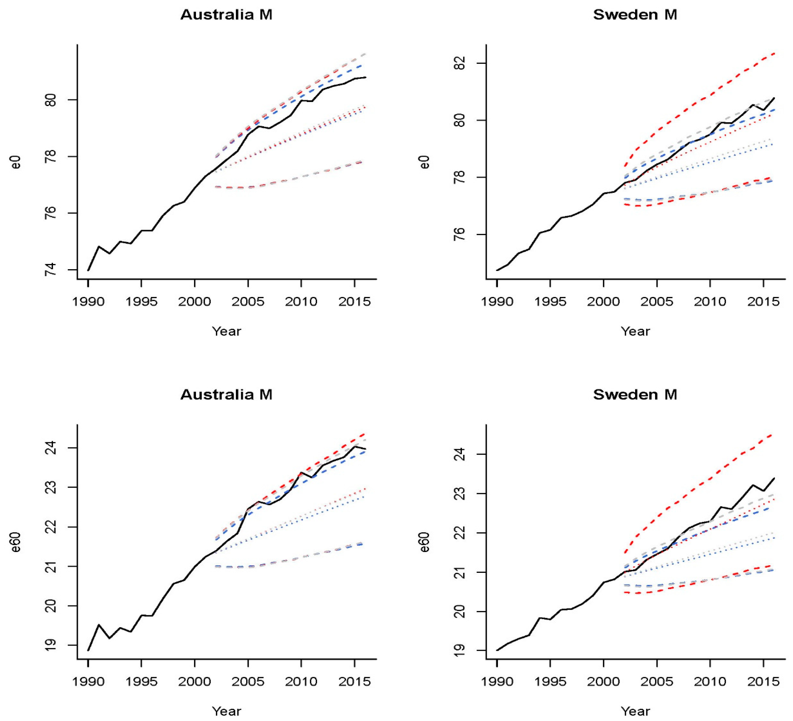
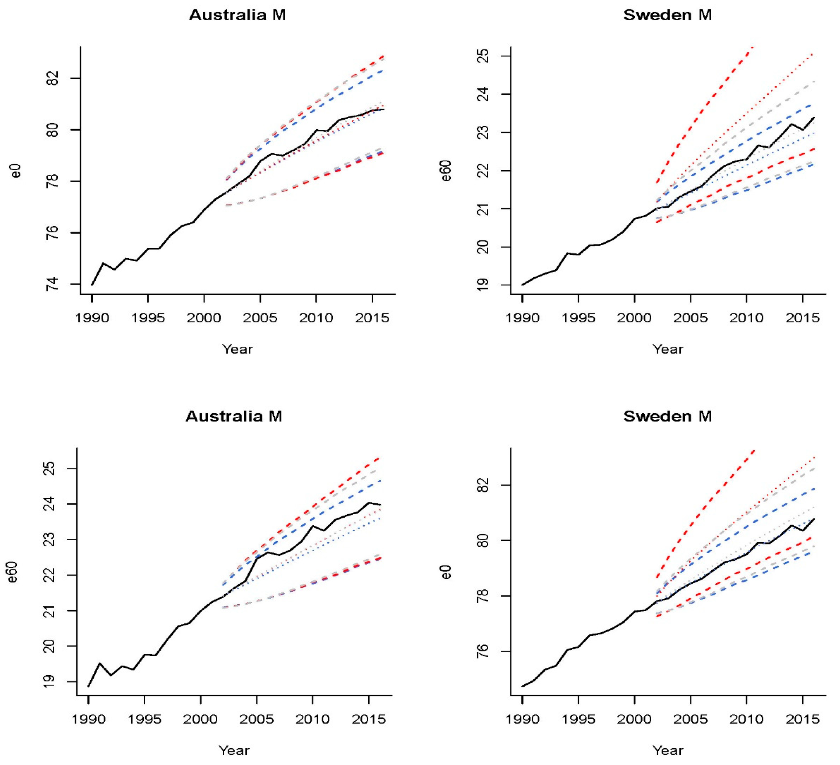
Recalling that Figure 7 depicts two representative examples, Australia and Sweden, the three sets of projections for the former presented an evident deviation from the observed trend, although the Fourier method seemed to capture the trend of the latter. We plot in Figure 10 the predicted life expectancies at age 0 and 60 of these two countries under the three mortality models with piecewise RWD. Interestingly, none of the historical $e_0$ and $e_{60}$ values of Swedish males fell outside the prediction intervals under the Fourier Lee-Carter model, both before and after introducing a piecewise RWD. As illustrated in the right column of Figure 10, arbitrarily introducing the time effects of structural changes to the Fourier Lee-Carter model (red dotted lines) might make life expectancy projections deviate from the observed trend. The results for Swedish male mortality data suggested that incorporating the Fourier time-varying age patterns alone or using the piecewise RWD alone was sufficient for generating the prediction intervals.

In summary, this section demonstrates that structural changes could not only be reflected in the overall mortality reduction trends, but could also be in the sensitivity to those changes at different ages. Two mortality models were proposed to capture the time-varying patterns of the age effects by fitting a Fourier-like (cubic-spline) process to the age sensitivity parameters in the original Lee-Carter model. For the six datasets tested, allowing for either the time-varying age sensitivity or the mortality index with breakpoints tends to improve backtesting results, and the integration of these two approaches was superior for five out of the six countries in this case.

6. Concluding Remarks

The presence of structural changes has been an issue in forecasting future mortality rates and life expectancies, especially when applying extrapolative mortality models. One representative among this category is the Lee-Carter model defined by a mortality index and two time-invariant age-specific parameters. Some analyses have been performed that allow structural shifts in period effects, but little attention has been paid to time-varying age effects whose potential existence has been identified by several authors (Lee and Miller 2000; van Berkum et al. 2016).

In this paper, we proposed modifications to the original Lee-Carter model to allow the age sensitivity parameters to change over time. Specifically, the Fourier series with time-varying amplitude and phase parameters was fitted to the age response to incorporate variations in these factors over time. For comparison, an alternative approach was considered that models the age patterns by cubic splines with time-varying coefficients. The forecasting performances of the Fourier Lee-Carter model, cubic Lee-Carter model and baseline Lee-Carter model were evaluated on the male mortality data of six countries. Our backtesting results showed that, on average, allowing for a changing Fourier (cubic) age response was likely to produce more accurate projections than using a constant age response, especially for older (middle-aged) ages. Moreover, the newly proposed models could generate wider prediction intervals by involving additional process error from the evolving age sensitivity factor. The widths of prediction intervals would be further influenced by the choice of time series processes fitted to the time-varying parameters of the age response.

We conducted a case study using the mortality data of the United Kingdom to illustrate the integration of structural changes in both the age and period effects. Our analysis suggested that taking full account of structural changes in mortality modelling tended to capture future mortality trends more accurately. Nevertheless, there were some exceptions where including structural breaks in the mortality index worsened the forecasting performance under the Lee-Carter model with time-varying age patterns. For Sweden, for instance, incorporating the age effects or time effects of structural changes alone would be sufficient to produce accurate forecasts of mortality rates, whereas the integration of both had the effect of exaggerating the impact of structural changes in this case. If the structural break in the mortality index was not significant, incorporating the age effects of structural changes alone would be adequate.

There are some possible directions of future research. We determined the split (knot) age and frequencies by considering the overall features of the age sensitivity factor over different subperiods. Other split choices might be adopted to enhance the performance of the proposed models. For instance, one might explore the optimal number and locations of age splits (number and positions of knots) for the Fourier (cubic) approach, but further investigation is needed. In addition, this paper evaluates model performances on male populations, although structural changes might occur differently for females (Coelho and Nunes 2011). It would be interesting to apply similar techniques as in the present paper to examine the structural changes for each sex. To ensure the mortality coherence of mortality projections between both sexes, one might modify the age sensitivity parameters in the augmented common factor model developed by Li and Lee (2005). Comparisons can be made between forecasts from the Fourier (cubic) Lee-Carter model with each sex modelled separately and a common factor model with a similar Fourier (cubic) adjustment with both sexes modelled jointly. Our study shows that a Fourier-like process can depict changes in the Lee-Carter age sensitivity parameter across ages 0-89 for Australia, Canada, New Zealand, Sweden, the United Kingdom and the United States. When different age groups are under interest, the proposed models might not necessarily be optimal. In this case, one might employ a Fourier series with functional coefficients without specifying the shape of the age response. The resulting mortality model with the parametric age function would offer more flexibility on modelling mortality age patterns. Ideally, it can accommodate features from different age ranges, sample periods, and populations.

References

1. Alho, Juha M. 2000. “The Lee-Carter Method for Forecasting Mortality, with Various Extensions and Applications”, Ronald Lee, January 2000. North American Actuarial Journal 4: 91–93. [Google Scholar] [CrossRef]
2. Amaral, Luiz Felipe, Reinaldo Castro Souza, and Maxwell Stevenson. 2008. A smooth transition periodic autoregressive (STPAR) model for short-term load forecasting. International Journal of Forecasting 24: 603–15. [Google Scholar] [CrossRef]
3. Armstrong, Ben. 2006. Models for the Relationship between Ambient Temperature and Daily Mortality. Epidemiology 17: 624–31. Available online: http://www.jstor.org.simsrad.net.ocs.mq.edu.au/stable/20486290 (accessed on 14 March 2020). [CrossRef] [PubMed]
4. Awad, Yaser, Shaul K. Bar-Lev, and Udi Makov. 2022. A New Class of Counting Distributions Embedded in the Lee–Carter Model for Mortality Projections: A Bayesian Approach. Risks 10: 111. [Google Scholar] [CrossRef]
5. Booth, Heather, Rob Hyndman, Leonie Tickle, and Piet de Jong. 2006. Lee-Carter mortality forecasting: A multi-country comparison of variants and extensions. Demographic Research 15: 289–310. Available online: https://EconPapers.repec.org/RePEc:dem:demres:v:15:y:2006:i:9 (accessed on 30 April 2020). [CrossRef]
6. Bracewell, Ronald N. 1978. The Fourier Transform and Its Applications, 2nd ed. New York: McGraw-Hill. [Google Scholar]
7. Brouhns, Natacha, Michel Denuit, and Jeroen K. Vermunt. 2002. A Poisson log-bilinear regression approach to the construction of projected lifetables. Insurance: Mathematics and Economics 31: 373–93. Available online: https://EconPapers.repec.org/RePEc:eee:insuma:v:31:y:2002:i:3:p:373-393 (accessed on 15 November 2019). [CrossRef] [Green Version]
8. Cairns, Andrew J. G., David Blake, and Kevin Dowd. 2006. A Two-Factor Model for Stochastic Mortality with Parameter Uncertainty: Theory and Calibration. Journal of Risk and Insurance 73: 687–718. [Google Scholar] [CrossRef]
9. Cairns, Andrew J. G., David Blake, Kevin Dowd, Guy D. Coughlan, David Epstein, Alen Ong, and Igor Balevich. 2009. A Quantitative Comparison of Stochastic Mortality Models Using Data From England and Wales and the United States. North American Actuarial Journal 13: 1–35. [Google Scholar] [CrossRef]
10. Canisius, Francis, Hugh Turral, and David J. Molden. 2007. Fourier analysis of historical NOAA time series data to estimate bimodal agriculture. International Journal of Remote Sensing 28: 5503–22. [Google Scholar] [CrossRef]
11. Carter, Lawrence R., and Alexia Prskawetz. 2001. Examining structural shifts in mortality using the Lee-Carter method. Methoden und Ziele 39. Available online: https://www.demogr.mpg.de/Papers/Working/wp-2001-007.pdf (accessed on 3 June 2022).
12. Coale, Aj, and Ee Kisker. 1990. Defects in data on old-age mortality in the United States: New procedures for calculating mortality schedules and life tables at the highest ages. In Asian and Pacific Population Forum. Honolulu: East-West Population Institute, vol. 4. [Google Scholar]
13. Coelho, Edviges, and Luis C. Nunes. 2011. Forecasting mortality in the event of a structural change. Journal of the Royal Statistical Society: Series A (Statistics in Society) 174: 713–36. [Google Scholar] [CrossRef]
14. Currie, Iain D., Maria Durban, and Paul H. Eilers. 2004. Smoothing and forecasting mortality rates. Statal Modelling An International Journal 4: 279–98. [Google Scholar] [CrossRef]
15. De Jong, Piet, and Leonie Tickle. 2006. Extending Lee–Carter Mortality Forecasting. Mathematical Population Studies 13: 1–18. [Google Scholar] [CrossRef]
16. Debón, Ana, Francisco Montes, and Ramón Sala. 2006. A Comparison of Nonparametric Methods in the Graduation of Mortality: Application to Data from the Valencia Region (Spain). International Statistical Review/Revue Internationale de Statistique 74: 215–33. Available online: http://www.jstor.org/stable/25472704 (accessed on 2 January 2020).
17. Dowd, Kevin, Andrew J. G. Cairns, David Blake, Guy D. Coughlan, David Epstein, and Marwa Khalaf-Allah. 2010. Backtesting Stochastic Mortality Models. North American Actuarial Journal 14: 281–98. [Google Scholar] [CrossRef]
18. Gampe, Jutta. 2010. Human mortality beyond age 110. In Supercentenarians. Edited by Heiner Maier, Jutta Gampe, Bernard Jeune, Jean-Marie Robine and James W. Vaupel. Berlin and Heidelberg: Springer, pp. 219–30. [Google Scholar]
19. Goyal, Amit, and Ivo Welch. 2003. Predicting the equity premium with dividend ratios. Management Science 49: 639–54. [Google Scholar] [CrossRef] [Green Version]
20. Gysen, Bart L. J., Esin Ilhan, Koen J. Meessen, Johannes J. H. Paulides, and Elena A. Lomonova. 2010. Modeling of Flux Switching Permanent Magnet Machines With Fourier Analysis. IEEE Transactions on Magnetics 46: 1499–502. [Google Scholar] [CrossRef] [Green Version]
21. Heligman, L., and J. H. Pollard. 1980. The age pattern of mortality. Journal of the Institute of Actuaries 107: 49–80. [Google Scholar] [CrossRef]
22. Human Mortality Database. 2019. University of California, Berkeley (USA), and Max Planck Institute for Demographic Research (Germany). Available online: www.mortality.org (accessed on 10 December 2019).
23. Inoue, Atsushi, Lu Jin, and Barbara Rossi. 2017. Rolling window selection for out-of-sample forecasting with time-varying parameters. Journal of econometrics 196: 55–67. [Google Scholar] [CrossRef] [Green Version]
24. Lee, R. Ronald, and Lawrence R. Carter. 1992. Modeling and Forecasting U.S. Mortality. Journal of the American Statistical Association 87: 659–71. [Google Scholar] [CrossRef]
25. Lee, Ronald, and Timothy Miller. 2000. Assessing the Performance of the Lee-Carter Approach to Modeling and Forecasting Mortality. Los Angeles: Annual Meeting of the Population Association of America. [Google Scholar]
26. Li, Jackie. 2013. A Poisson common factor model for projecting mortality and life expectancy jointly for females and males. Population Studies 67: 111–26. [Google Scholar] [CrossRef]
27. Li, Nan, and Ronald Lee. 2005. Coherent Mortality Forecasts for a Group of Populations: An Extension of the Lee-Carter Method. Demography 42: 575–94. Available online: http://www.jstor.org/stable/4147363 (accessed on 5 November 2019). [CrossRef] [PubMed] [Green Version]
28. Li, Jackie, and Kenneth Wong. 2020. Incorporating structural changes in mortality improvements for mortality forecasting. Scandinavian Actuarial Journal 2020: 776–91. [Google Scholar] [CrossRef]
29. Li, Johnny S.-H., Wai-Sum Chan, and Siu-Hung Cheung. 2011. Structural Changes in the Lee-Carter Mortality Indexes. North American Actuarial Journal 15: 13–31. [Google Scholar] [CrossRef]
30. Li, Nan, Ronald Lee, and Patrick Gerland. 2013. Extending the Lee-Carter method to model the rotation of age patterns of mortality decline for long-term projections. Demography 50: 2037–51. [Google Scholar] [CrossRef] [Green Version]
31. Lombardet, Benoît, L. Andrea Dunbar, Rolando Ferrini, and Romuald Houdré. 2005. Fourier analysis of Bloch wave propagation in photonic crystals. Journal of the Optical Society of America B 22: 1179–90. [Google Scholar] [CrossRef]
32. Mei, Liang, and Sune Svanberg. 2015. Wavelength modulation spectroscopy—Digital detection of gas absorption harmonics based on Fourier analysis. Applied Optics 54: 2234–43. [Google Scholar] [CrossRef]
33. Milidonis, Andreas, Yijia Lin, and Samuel H. Cox. 2011. Mortality Regimes and Pricing. North American Actuarial Journal 15: 266–89. [Google Scholar] [CrossRef]
34. O’Hare, Colin, and Youwei Li. 2015. Identifying Structural Breaks in Stochastic Mortality Models. ASCE-ASME Journal of Risk and Uncertainty in Engineering Systems, Part B: Mechanical Engineering 1: 021001. [Google Scholar] [CrossRef]
35. Perron, Pierre. 1989. The great crash, the oil price shock, and the unit root hypothesis. Econometrica: Journal of the Econometric Society 57: 1361–401. [Google Scholar] [CrossRef]
36. Pitt, David, Jackie Li, and Tian Kang Lim. 2018. Smoothing Poisson common factor model for projecting mortality jointly for both sexes. ASTIN Bulletin: The Journal of the IAA 48: 509–41. [Google Scholar] [CrossRef]
37. Powers, Michael R., and Thomas Y. Powers. 2015. Fourier-analytic measures for heavy-tailed insurance losses. Scandinavian Actuarial Journal 2015: 527–47. [Google Scholar] [CrossRef]
38. Sweeting, Paul J. 2011. A Trend-Change Extension of the Cairns-Blake-Dowd Model. Annals of Actuarial Science 5: 143–62. [Google Scholar] [CrossRef]
39. van Berkum, Frans, Katrien Antonio, and Michel Vellekoop. 2013. Structural Changes in Mortality Rates with an Application to Dutch and Belgian Data. FEB Research Report AFI-1379: 1–27. [Google Scholar] [CrossRef]
40. van Berkum, Frans, Katrien Antonio, and Michel Vellekoop. 2016. The impact of multiple structural changes on mortality predictions. Scandinavian Actuarial Journal 2016: 581–603. [Google Scholar] [CrossRef]
41. Vyas, Seema, and Lilani Kumaranayake. 2006. Constructing socio-economic status indices: How to use principal components analysis. Health Policy and Planning 21: 459–68. [Google Scholar] [CrossRef] [Green Version]
42. Wong, Jackie S. T., Jonathan J. Forster, and Peter W. F. Smith. 2018. Bayesian mortality forecasting with overdispersion. Insurance: Mathematics and Economics 83: 206–21. [Google Scholar] [CrossRef] [Green Version]
Figure 1. Age sensitivity factors under the Lee-Carter model estimated from sequential subsamples with a fixed sample size.
Risks 10 00147 g001
Figure 2. Modelling process of Fourier parameters for the age sensitivity factors.
Risks 10 00147 g002
Figure 3. Age sensitivity factors under the Lee-Carter model estimated from sequential subperiods (using the same set of mortality level and mortality index parameters). The legend b [ x , t ] refers to the age response β x calibrated on a subperiod ending in year t .
Risks 10 00147 g003
Figure 4. Curves of sin ( x + P t ( i ) ) for different phase values. The left (right) column indicates possible shapes for the Fourier series before (after) the splitting age. The parts on the left of the two black dashed (vertical) lines in the left and right plots denote the shape of a quarter and half of a complete cycle, respectively.
Risks 10 00147 g004
Figure 5. Estimated (solid lines) and fitted (dashed lines) age sensitivity factor under the Lee-Carter model estimated from the latest 24-year subperiod. The blue (red) lines refer to fitted values using the Fourier (cubic-spline) method.
Risks 10 00147 g005
Figure 6. Observed (blue lines) and projected (black lines) life expectancy at birth ( e 0 ), calibrated on mortality data from the whole sample period. The solid lines correspond to forecasts under the original Lee-Carter model. The dashed and dotted lines refer to projections from the Fourier Lee-Carter model and cubic Lee-Carter model, respectively.
Risks 10 00147 g006
Figure 7. Observed values (solid lines), projected values (dotted lines) and 95% prediction intervals (dashed lines) of life expectancies at birth (top panel) and age 60 (bottom panel), calibrated on years 1950–2001. The blue lines correspond to the projections from the original Lee-Carter model, and the red (grey) lines refer to the projections from the Fourier (cubic) Lee-Carter model.
Risks 10 00147 g007
Figure 8. Parameter estimates of mortality index k t under the original Lee-Carter model for the United Kingdom, calibrated on years 1950–2001. The red dashed line is based on two random walk processes connected at a breakpoint. The blue dashed line is based on a single random walk process over the whole fitting period.
Risks 10 00147 g008
Figure 9. Observed values (solid lines), projected values (dotted lines), and 95% prediction intervals (dashed lines) of life expectancies at ages 0 (panel (a)) and 60 (panel (b)) for the United Kingdom, calibrated on years 1950–2001.
Risks 10 00147 g009
Figure 10. Observed values (solid lines), projected values (dotted lines) and 95% prediction intervals (dashed lines) of life expectancies at birth (top panel) and age 60 (bottom panel), calibrated on years 1950-2001. The blue lines correspond to the projections from the original Lee-Carter model, and the red (grey) lines refer to the projections from the Fourier (cubic) Lee-Carter model. The mortality index is modelled as piecewise RWD.
Risks 10 00147 g010