Pricing Energy Derivatives in Markets Driven by Tempered Stable and CGMY Processes of Ornstein–Uhlenbeck Type

Abstract

In this study, we consider the pricing of energy derivatives when the evolution of spot prices follows a tempered stable or a CGMY-driven Ornstein–Uhlenbeck process. To this end, we first calculate the characteristic function of the transition law of such processes in closed form. This result is instrumental for the derivation of nonarbitrage conditions such that the spot dynamics is consistent with the forward curve. Moreover, we also conceive efficient algorithms for the exact simulation of the skeleton of such processes and propose a novel procedure when they coincide with compound Poisson processes of Ornstein–Uhlenbeck type. We illustrate the applicability of the theoretical findings and the simulation algorithms in the context of pricing different contracts, namely strips of daily call options, Asian options with European style and swing options.

1. Introduction

Most energy and commodity markets exhibit seasonality, mean-reversion high volatilities and occasional distinctive price spikes, which results in demand for derivative products which protect the holder against high prices. In equity markets, there is clear evidence that asset returns are not Gaussian and it is common practice to rely on Lévy processes, other than the Brownian motion, in order to capture heavy-tails and jumps of the log-prices. Several empirical studies (see for instance Carr and Crosby 2010) have shown that the CGMY Lévy processes introduced by Carr et al. (2002), named after its authors, are a valuable alternative. Moreover, the class of such processes is quite flexible and also encompasses variance gamma processes introduced in Madan and Seneta (1990) and is, on the other hand, a special case of the wider class of bilateral tempered stable processes (see Küchler and Tappe 2013), which in turn represent an alternative to normal inverse Gaussian models (see Barndorff-Nielsen 1998 and Cont and Tankov 2004).

Commodity and energy markets, however, exhibit mean reversion which cannot be described by plain Lévy processes but rather by Lévy-driven Ornstein–Uhlenbeck (OU) processes. In a series of papers, Sabino (2020a) and Sabino and Cufaro Petroni (2021a, 2022) study the analogous of variance gamma and tempered stable processes of OU type. In particular in this latter case, Sabino and Cufaro Petroni (2022) details the exact simulation of tempered stable subordinators only. Following this route, in this study, we consider the pricing of energy derivatives assuming that the spot price is driven by CGMY and tempered stable processes of OU type. The first novel contribution consists in the derivation of the closed formula of the characteristic function of the transition law of these processes that is instrumental to find nonarbitrage conditions. It also gives the fundamental ingredient to calculate the price of financial derivatives with FFT-based methods.

The second contribution is the extension of the exact methods for the simulation of the skeleton of tempered stable processes of OU type to the case of finite activity, hence compound Poisson processes of OU type, but also to the bilateral and the CGMY cases.

We then illustrate the applicability of our findings and the proposed simulation algorithms to the pricing of a few energy derivative contracts. As a first application, we consider the pricing of a daily strip of call options on the day-ahead spot price driven by tempered stable OU processes using the FFT technique of Carr and Madan (1999). Secondly, we consider the pricing of Asian options depending on the day-ahead spot price described by a CGMY-driven OU process via Monte Carlo simulations. In this case, we calibrate the model parameters to realistic data, namely to the historical gas spot prices in Italy (PSV) and we also highlight the differences between our exact simulation schemes and two approximate procedures. The last example consists in pricing swing options with the modified version of the Least-Squares Monte Carlo method detailed in Boogert and de Jong (2008, 2011) using market models based on a CGMY-driven OU process that coincides with compound Poisson processes of OU type.

The paper is organized as follows. Section 2 introduces tempered stable and CGMY processes and the general results relative to Lévy-driven OU processes. In Section 3, we focus on the classical tempered stable and CGMY processes of OU type with finite variation and derive the characteristic function of their transition law. In Section 4, we present the algorithms for the simulation of the skeleton of the processes under study and we focus on the case of compound Poisson processes of OU type. We also present numerical experiments demonstrating their efficiency. The application of these results is illustrated in Section 5 in the context of the pricing of energy derivative contracts, namely daily strips of call options, Asian options with European exercise and swing options written on the day-ahead spot price. Finally, Section 6 concludes the paper with an overview of future inquiries and possible further applications.

Notation

Before proceeding, we introduce some notation and shortcuts that are used throughout the paper. We write $\mathrm{\Gamma }(\alpha ,\beta )$ to denote the gamma distribution with shape parameter $\alpha >0$ and rate parameter $\beta >0$. Moreover, we write $\mathcal{U}\left(\right[0,1\left]\right)$ to denote the uniform distribution in $[0,1]$ and $\mathcal{P}\left(\lambda \right)$ to denote the Poisson distribution with parameter $\lambda >0$. We use the shortcuts id and sd for infinitely divisible and self-decomposable distributions, respectively. We use the shortcut rv for random variable and iid for independently and identically distributed, whereas we use chf, lch  cgf and pdf as shortcuts for characteristic function, logarithmic characteristic, cumulant generating function and density function, respectively.

2. Preliminaries

Take a Lévy process $L(·)$ of classic tempered stable type, namely with the Lévy measure having density

$$\nu \left(x\right)={\nu }_p\left(x\right)+{\nu }_x\left(x\right)=c_p\frac{e^{-{\beta }_{p}x}}{x^{1+{\alpha }_p}}{\mathrm{𝟙}}_{x\ge 0}+c_n\frac{e^{{\beta }_{n}x}}{{\left|x\right|}^{1+{\alpha }_n}}{\mathrm{𝟙}}_{x<0}$$

(1)

where $c_p,c_n,{\beta }_p$ and ${\beta }_n$ are all positive numbers, ${\alpha }_p<2$ and ${\alpha }_n<2$. Hereafter, we denote with $\mathcal{BCTS}({\alpha }_p,{\alpha }_n,{\beta }_p,{\beta }_n,c_{p}t,c_{n}t)$ the law of $L\left(t\right)$.

Different applications of such a process can be found among others in Koponen (1995), Carr et al. (2002), Poirot and Tankov (2006) and Ballotta and Kyriakou (2014). In particular, the model introduced in Carr et al. is named CGMY and assumes $C=c_p=c_n$, $Y={\alpha }_p={\alpha }_n$, $G={\beta }_n$ and $M={\beta }_p$ from the names of the authors. It can also be proven that a classic tempered stable process is a time-changed Brownian motion provided $c_p=c_n$ and ${\alpha }_p={\alpha }_n=\alpha >-1$ (see Proposition 4.1 of Cont and Tankov 2004). For sake of completeness, it is worthwhile mentioning that we are referring to classic tempered stable processes because different processes can be constructed applying an alternative tempering function rather than the exponential function used in (1) (see Rosinski 2007). An overview of such processes, named general tempered stable processes, can be found in Grabchak (2016).

In the following, we consider the subset of classic tempered stable processes with no drift and with finite variation for which it holds ${\alpha }_p<1$ and ${\alpha }_n<1$, and in particular when ${\alpha }_p<0$ and ${\alpha }_n<0$, the subset consists of Poisson processes (see Cont and Tankov 2004). Due to the fact that any process of finite variation can be seen as the difference of two independent subordinators, the process $L(·)$ can be written as $L\left(t\right)=L_p\left(t\right)-L_n\left(t\right)$, where $L_p(·)$ and $L_n(·)$ are two classic tempered stable subordinators with Lévy densities ${\nu }_p\left(x\right)$ and ${\nu }_n(-x)$, respectively. In the following, we dub classic tempered stable subordinators with CTS, whereas the full bilateral case is denoted with BCTS. Moreover, we denote the marginal law of a CTS subordinator at time t with $\mathcal{CTS}(\alpha ,\beta ,ct)$.

Consider now an Ornstein–Uhlenbeck (OU) process $X(·)$ solution of the stochastic differential equation

$$\begin{array}{ccc}\hfill dX\left(t\right)& =& -bX\left(t\right)dt+dL\left(t\right),X\left(0\right)=X_0\mathit{P}\text{-}a.s.b>0\hfill \end{array}$$

(2)

namely,

$$\begin{array}{ccc}\hfill X\left(t\right)& =& X_0{e}^{-bt}+Z\left(t\right),Z\left(t\right)={\int }_0^t{e}^{-b(t-s)}dL\left(s\right),\hfill \end{array}$$

(3)

$$\begin{array}{ccc}\hfill Z\left(t\right)& =& Z_p\left(t\right)-Z_n\left(t\right),Z_d\left(t\right)={\int }_0^t{e}^{-b(t-s)}d{L}_d\left(s\right),d\in \{p,n\}.\hfill \end{array}$$

(4)

Following the convention in Barndorff-Nielsen and Shephard (2001), $X(·)$ is then named OU-BCTS process or, if the above parameter constrain holds, OU-CGMY process.

There is a close relation between the concept of self-decomposability and the theory of Lévydriven OU processes, indeed as observed in Barndorff-Nielsen et al. (1998), the solution process (3) is stationary if and only if its chf ${\phi }_X(u,t)$ is constant in time and steadily coincides with the chf ${\overline{\phi }}_X\left(u\right)$ of the sd invariant initial distribution that turns out to be decomposable according to

$${\overline{\phi }}_X\left(u\right)={\overline{\phi }}_X\left(u{e}^{-bt}\right){\phi }_Z(u,t)$$

where now, at every given t, ${\phi }_Z(u,t)=e^{{\psi }_Z(u,t)}$ denotes the id chf of the rv $Z\left(t\right)$ in (3) and ${\psi }_Z(u,t)$ its lch. We remark that the process $Z(·)$ is neither a Lévy process nor an additive process, however, as we clarify in the following, the law of the rv $Z\left(t\right)$ is id.

We recall here that a law with chf $\eta \left(u\right)$ is said to be sd (see Sato 1999; Cufaro Petroni 2008) when for every $0<a<1$ we can find another law with chf ${\chi }_a\left(u\right)$ such that

$$\eta \left(u\right)=\eta \left(au\right){\chi }_a\left(u\right).$$

(5)

Of course a rv X with chf $\eta \left(u\right)$ is also said to be sd when its law is sd, and looking at the definitions, this means that for every $0<a<1$ we can always find two independent rv’s—a Y with the same law of X and a $Z_a$ with chf ${\chi }_a\left(u\right)$—such that in distribution

$$X\stackrel{d}{=}aY+Z_a.$$

(6)

Hereafter, the rv $Z_a$ is called the a-remainder of X, and in general it has an id distribution (see Sato 1999).

This last statement apparently means that the law of $Z\left(t\right)$ in the solution (3) coincides with that of the a-remainder of the sd, stationary law ${\overline{\phi }}_X$, provided that $a=e^{-bt}$. Therefore, one can rely on the results relative to id laws to study the properties of the rv $Z\left(t\right)$.

It is easy indeed to see from (3) that the chf of the time homogeneous transition law with a degenerate initial condition $X\left(0\right)=x_0,\mathit{P}\text{-}a.s.$ is

$${\phi }_X(u,t|x_0)=e^{i{x}_{0}u{e}^{-bt}}{\phi }_Z(u,t)=\frac{{\overline{\phi }}_X\left(u\right)e^{i{x}_{0}u{e}^{-bt}}}{{\overline{\phi }}_X\left(u{e}^{-bt}\right)}$$

(7)

moreover, we have

$${\psi }_Z(u,t)={\psi }_{Z_p}\left(u\right)+{\psi }_{Z_n}(-u),$$

(8)

and

$${\psi }_X(u,t|x_0)=iu{x}_0{e}^{-bt}+{\psi }_Z(u,t)=iu{x}_0{e}^{-bt}+{\psi }_{Z_p}(u,t)+{\psi }_{Z_n}(-u,t)$$

(9)

where ${\psi }_{Z_d}(u,t)=\ln {\phi }_{Z_d}(u,t),d\in \{p,n\}$ is the lch of $Z_d\left(t\right),d\in \{p,n\}$. Moreover, the transition lch of a OU process can also be written in terms of the corresponding ${\psi }_L\left(u\right)$ in the form

$${\psi }_X(u,t|x_0)=iu{x}_0{e}^{-bt}+{\psi }_Z(u,t)=iu{x}_0{e}^{-bt}+{\int }_0^t{\psi }_L\left(u{e}^{-bs}\right)ds.$$

(10)

Finally, in virtue of the results of Sabino and Cufaro Petroni (2022), one can relate the Lévy density ${\nu }_Z(x,t)$ of $Z\left(t\right)$ to that of the BDLP $L(·)$ at $t=1$ denoted with ${\nu }_L\left(x\right)$

$$\begin{array}{ccc}\hfill {\nu }_Z(x,t)& =& \frac{1}{b\left|x\right|}\left\{\begin{array}{cc}{\int }_{{}^x{/}_a}^x{\nu }_L\left(y\right)dy\hfill & x<0\hfill \\ \\ {\int }_x^{{}^x{/}_a}{\nu }_L\left(y\right)dy\hfill & x>0\hfill \end{array}\right.a=e^{-bt}.\hfill \end{array}$$

(11)

3. OU-BCTS and OU-CGMY Processes

In this section, we study OU-BCTS and OU-CGMY processes with finite variation and distinguish the case where the BDLP is of infinite activity, $0<{\alpha }_p<1$ and $0<{\alpha }_n<1$, to that of finite activity, namely when $Z(·)$ is a compound Poisson process. We do not discuss the setting ${\alpha }_p={\alpha }_n=0$ because it is already covered in Sabino (2020a) and corresponds to a variance gamma-driven OU process, therefore of infinite activity and finite variation.

3.1. Infinite Activity

Apparently, the study of the transition law of a OU-BCTS process $X(·)$ coincides with the study of the process $Z(·)$, and in particular of the processes $Z_p(·)$ and $Z_n(·)$, defined in (4). One of course can rely on these last two processes to build OU-BCTS processes.

Sabino and Cufaro Petroni (2022) and Qu et al. (2021) designed an exact decomposition of the transition law of OU-CTS processes as the convolution of two independent rv’s plus a degenerate term. For simplicity, we report this result here below in addition because such a OU process is driven by a CTS subordinator, and we consider only $Z_p(·)$.

Proposition 1.

For $0<{\alpha }_p<1$, and at every $t>0$, the solution of an OU-CTS Equation (3) with $X\left(0\right)=X_0,\mathit{P}\text{-}a.s.$ is in distribution the sum of three independent rv’s

$$X\left(t\right)=a{X}_0+Z_p\left(t\right)\stackrel{d}{=}a{X}_0+X_1+X_{2}a=e^{-bt}$$

(12)

where $X_1$ is distributed according to the law $\mathcal{CTS}\left({\alpha }_p,\frac{{\beta }_p}{a},c_p\frac{1-a_p^{\alpha }}{{\alpha }_{p}b}\right)$, whereas

$$X_2=\sum _{k=1}^{N_a}{J}_k$$

is a compound Poisson rv where $N_a$ is an independent Poisson rv with parameter

$${\mathrm{\Lambda }}_a=\frac{c_p{\beta }_p^{{\alpha }_p}\mathrm{\Gamma }(1-{\alpha }_p)}{b{\alpha }_p^2{a}^{{\alpha }_p}}\left(1-a^{{\alpha }_p}+a^{{\alpha }_p}\log a^{{\alpha }_p}\right)$$

(13)

and $J_k,k>0$ are iid rv’s with density

$$f_J\left(x\right)=\frac{{\alpha }_p{a}^{{\alpha }_p}}{1-a_p^{\alpha }+a^{{\alpha }_p}\log a^{{\alpha }_p}}{\int }_1^{\frac{1}{a}}\frac{x^{-{\alpha }_p}{\left({\beta }_{p}v\right)}^{1-{\alpha }_p}{e}^{-{\beta }_{p}vx}}{\mathrm{\Gamma }(1-{\alpha }_p)}\frac{v^{{\alpha }_p}-1}{v}dv$$

(14)

namely, a mixture of a gamma law and a distribution with density

$$f_V\left(v\right)=\frac{{\alpha }_p{a}_p^{\alpha }}{1-a^{{\alpha }_p}+a^{{\alpha }_p}\log a^{{\alpha }_p}}\frac{v^{{\alpha }_p}-1}{v}1\le v\le {}^1{/}_a.$$

(15)

The extension to the bilateral OU-BCTS process is straightforward, for instance, the simulation algorithms consist of repeating the procedure for an OU-CTS process two times.

The main contribution of this subsection is the derivation of the lch and hence the chf and the moment-generating function of $Z\left(t\right)$ that is instrumental to find the risk neutral conditions for market models based on OU-BCTS processes and to the pricing of derivative contracts using FFT methods.

Proposition 2.

The lch ${\psi }_{Z_p}(u,t)$, $u\in \mathbb{R}$ with $0<{\alpha }_p<1$ can be represented as:

$${\psi }_{Z_p}(u,t)=-\frac{c_p{\beta }_p^{{\alpha }_p}\mathrm{\Gamma }(1-{\alpha }_p)}{{\alpha }_{p}b}\left[I\left(u,{\alpha }_p,{\beta }_p,\frac{{\beta }_p}{a}\right)+\log a\right],a=e^{-bt}$$

(16)

with

$$\begin{array}{ccc}\hfill I\left(u,\alpha ,{\beta }_1,{\beta }_2\right)& =& {\int }_{{\beta }_1}^{{\beta }_2}{z}^{-1-\alpha }{(z-iu)}^{\alpha }dz\hfill \\ & =& -\frac{1}{\alpha }\left[{\left(\frac{u}{i{\beta }_2}\right)}^{\alpha }{}_2{F}_1\left(-\alpha ,-\alpha ,1-\alpha ,-\frac{i{\beta }_2}{u}\right)\right.-\hfill \\ & & \left.{\left(\frac{u}{i{\beta }_1}\right)}^{\alpha }{}_2{F}_1\left(-\alpha ,-\alpha ,1-\alpha ,-\frac{i{\beta }_1}{u}\right)\right]\hfill \end{array}$$

(17)

where ${}_2{F}_1(a,b,c,x)$ is the hypergeometric function, $0<\alpha <1$, ${\beta }_1>0$ and ${\beta }_2>0$.

Proof. 

From (11) it also results

$${\nu }_{Z_p}(x,t)=\frac{c_p}{bx}{\int }_x^{\frac{x}{a}}\frac{e^{-{\beta }_{p}y}}{y^{{\alpha }_p+1}}dy=\frac{c_p}{b}{\int }_1^{\frac{1}{a}}\frac{e^{-{\beta }_{p}wx}}{x^{{\alpha }_p+1}{w}^{{\alpha }_p+1}}dw$$

therefore, because of the Lévy-Khintchin theorem

$${\psi }_{Z_p}(u,t)=\frac{1}{b}{\int }_1^{\frac{1}{a}}{w}^{-{\alpha }_p-1}dw{\int }_0^{\infty }{c}_p\left(e^{iux}-1\right)\frac{e^{-{\beta }_{p}wx}}{x^{{\alpha }_p+1}}dx$$

The second integral is the lch of a $\mathcal{CTS}({\alpha }_p,{\beta }_p,c_p)$ law with $0<{\alpha }_p<1$, and from Lemma 2.5 of Küchler and Tappe (2013) we have

$$\begin{array}{ccc}\hfill {\psi }_{Z_p}(u,t)& =& \frac{c_p\mathrm{\Gamma }(-{\alpha }_p)}{b}{\int }_1^{\frac{1}{a}}\frac{{\left({\beta }_{p}w-iu\right)}^{{\alpha }_p}-{\left({\beta }_{p}w\right)}^{{\alpha }_p}}{w^{{\alpha }_p+1}}dw\hfill \\ & =& \frac{c_p\mathrm{\Gamma }(-{\alpha }_p)}{b}\left[{\int }_1^{\frac{1}{a}}\frac{{\left({\beta }_{p}w-iu\right)}^{{\alpha }_p}}{w^{{\alpha }_p+1}}dw-{\beta }_p^{{\alpha }_p}{\int }_1^{\frac{1}{a}}\frac{dw}{w}\right]\hfill \\ & =& -\frac{c_p{\beta }_p^{\alpha }\mathrm{\Gamma }(1-{\alpha }_p)}{\alpha b}\left[{\int }_{{\beta }_p}^{\frac{{\beta }_p}{a}}{z}^{-1-{\alpha }_p}{(z-iu)}^{{\alpha }_p}dz+\log a\right]\hfill \end{array}$$

where, of course, $-{\alpha }_p\mathrm{\Gamma }(-{\alpha }_p)=\mathrm{\Gamma }(1-{\alpha }_p)$, and in the last step we used the change in variables ${\beta }_{p}w=z$. In order to conclude the proof, we first observe that under the special case $\gamma =\alpha +1$ the derivative of the hypergeometric function is

$$\frac{d}{dz}{}_2{F}_1\left(\alpha ,\beta ,\alpha +1,z\right)=\frac{d}{dz}{}_2{F}_1(\beta ,\alpha ,\alpha +1,z)=-\frac{\alpha \left({(1-z)}^{\beta }-{}_2{F}_1(\alpha ,\beta ,\alpha +1,z\right))}{z}$$

then, with some algebra, we obtain

$$\frac{d}{dz}\left(z^{-\alpha }{}_2{F}_1\left(-\alpha ,-\alpha ,1-\alpha ,-\frac{iz}{u}\right)\right)=\alpha {\left(\frac{i}{u}\right)}^{\alpha }{z}^{\alpha +1}\left(z-iu\right),$$

therefore, we can write the integral

$$\begin{array}{ccc}\hfill I\left(u,\alpha ,{\beta }_p,\frac{{\beta }_p}{a}\right)& =& -\frac{1}{\alpha }\left[{\left(\frac{au}{i{\beta }_p}\right)}^{\alpha }{}_2{F}_1\left(-\alpha ,-\alpha ,1-\alpha ,-\frac{i{\beta }_2}{au}\right)\right.-\hfill \\ & & \left.{\left(\frac{u}{i{\beta }_p}\right)}^{\alpha }{}_2{F}_1\left(-\alpha ,-\alpha ,1-\alpha ,-\frac{i{\beta }_p}{u}\right)\right]\hfill \end{array}$$

as claimed.  □

Remark 1.

Several transformation and recursion formulas are applicable to the hypergeometric functions. Using 9.131.1 in Gradshteyn and Ryzhik (2007), we have

$${}_2{F}_1(-\alpha ,-\alpha ,1-\alpha ,x)={(1-x)}^{\alpha +1}{}_2{F}_1(1,1,1-\alpha ,x)$$

and accordingly, (17) becomes

$$\begin{array}{ccc}\hfill I\left(u,\alpha ,{\beta }_1,{\beta }_2\right)& =& -\frac{i}{\alpha u}\left[{\beta }_2^{-\alpha }{\left({\beta }_2-iu\right)}^{\alpha +1}{}_2{F}_1\left(1,1,1-\alpha ,-\frac{i{\beta }_2}{u}\right)\right.-\hfill \\ & & \left.{\beta }_1^{-\alpha }{\left({\beta }_1-iu\right)}^{\alpha +1}{}_2{F}_1\left(1,1,1-\alpha ,-\frac{i{\beta }_1}{u}\right)\right].\hfill \end{array}$$

(18)

Corollary 1.

The cgf $m_{Z_p}(s,t)=\ln \mathit{E}\left[e^{s{Z}_p\left(t\right)}\right]$ of $Z_p\left(t\right)$ with $0<{\alpha }_p<1$ exists for $s<{\beta }_p$ and is:

$$m_{Z_p}(s,t)=-\frac{c{\beta }_p^{{\alpha }_p}\mathrm{\Gamma }(1-{\alpha }_p)}{{\alpha }_{p}b}\left[\tilde{I}\left(s,{\alpha }_p,{\beta }_p,\frac{{\beta }_p}{a}\right)+\log a\right]s<{\beta }_p$$

(19)

where

$$\begin{array}{ccc}\hfill \tilde{I}\left(s,\alpha ,{\beta }_1,{\beta }_2\right)& =& {\int }_{{\beta }_1}^{{\beta }_2}{z}^{-1-\alpha }{(z-s)}^{\alpha }dz=\hfill \\ & & \frac{1}{\alpha s}\left[{\beta }_2^{-\alpha }{\left({\beta }_2-s\right)}^{\alpha +1}{}_2{F}_1\left(1,1,1-\alpha ,\frac{{\beta }_2}{s}\right)\right.-\hfill \\ & & \left.{\beta }_1^{-\alpha }{\left({\beta }_1-s\right)}^{\alpha +1}{}_2{F}_1\left(1,1,1-\alpha ,\frac{{\beta }_1}{s}\right)\right].\hfill \end{array}$$

(20)

Note that setting ${\psi }_{Z_p}(-is,t)=m_{Z_p}(s,t)$ in (17), one may claim that the cgf assumes complex values, which is obviously wrong, and it explains why we have preferred to rely on (18) to write (20).

In virtue of (8), Proposition 2 and Corollary 1 can be easily extended to cope with $Z\left(t\right)$ defined for OU-BCTS processes.

Corollary 2.

For a OU-BCTS process, the lch ${\psi }_Z(u,t)$, $u\in \mathbb{R}$ can be represented as:

$$\begin{array}{ccc}\hfill {\psi }_Z(u,t)& =& -\frac{c_p{\beta }_p^{{\alpha }_p}\mathrm{\Gamma }(1-{\alpha }_p)}{{\alpha }_{p}b}\left[I\left(u,{\alpha }_p,{\beta }_p,\frac{{\beta }_p}{a}\right)+\log a\right]-\hfill \\ & & \frac{c{\beta }_n^{{\alpha }_n}\mathrm{\Gamma }(1-{\alpha }_n)}{{\alpha }_{n}b}\left[I\left(-u,{\alpha }_n,{\beta }_n,\frac{{\beta }_n}{a}\right)+\log a\right].\hfill \end{array}$$

(21)

Accordingly,

Corollary 3.

The cgf at time t exists for $-{\beta }_n<s<{\beta }_p$ and is:

$$\begin{array}{ccc}\hfill m_Z(s,t)& =& -\frac{c{\beta }_p^{{\alpha }_p}\mathrm{\Gamma }(1-{\alpha }_p)}{{\alpha }_{p}b}\left[\tilde{I}\left(s,{\alpha }_p,{\beta }_p,\frac{{\beta }_p}{a}\right)+\log a\right]-\hfill \\ & & \frac{c{\beta }_n^{{\alpha }_n}\mathrm{\Gamma }(1-{\alpha }_n)}{{\alpha }_{n}b}\left[\tilde{I}\left(-s,{\alpha }_n,{\beta }_n,\frac{{\beta }_n}{a}\right)+\log a\right].\hfill \end{array}$$

(22)

Remark 2.

In contrast to Proposition 1 that is valid under the condition $0<{\alpha }_p<1$, we show in the next subsection that Proposition 2 and consequently all corollaries are also valid for ${\alpha }_p<0$ and ${\alpha }_n<0$ as well.

3.2. Finite Activity

When ${\alpha }_p<0$, the BDLP of a CTS process turns out to be a compound Poisson process; indeed, the integral of the Lévy density is convergent. In more detail, we have:

$${\int }_0^{\infty }{\nu }_{L_p}\left(x\right)dx=c_p{\int }_0^{\infty }{x}^{-{\alpha }_p-1}{e}^{-{\beta }_{p}x}dx=c_p\mathrm{\Gamma }(-{\alpha }_p){\beta }_p^{-{\alpha }_p}={\lambda }_p$$

(23)

where now $-\alpha$ is positive. It results then that

$$L_p\left(t\right)=\sum _{k=0}^{N_p\left(t\right)}{J}_k,J_0=0, \mathit{P}\text{-}a.s.,$$

(24)

where $N_p\left(t\right)$ is a Poisson process with the intensity ${\lambda }_p$ defined in (23) and jumps sizes $J_k$ independent of $N_p\left(t\right)$ distributed according to a gamma law with shape parameter $-{\alpha }_p$ and rate parameter ${\beta }_p$; indeed, the pdf of each copy of $J_k$ is

$$f_J\left(x\right)=\frac{{\nu }_L\left(x\right)}{\lambda }=\frac{{\beta }_p^{-{\alpha }_p}{x}^{-{\alpha }_p-1e^{-{\beta }_{p}x}}}{\mathrm{\Gamma }(-{\alpha }_p)},x>0.$$

This last representation is consistent with Jørgensen (1997), who observed that a compound Poisson process with gamma-distributed jumps follows a Tweedie distribution that is actually a CTS law.

Proposition 3.

For ${\alpha }_p<0$, and at every $t>0$, the solution of an OU-CTS Equation (3) with $X\left(0\right)=X_0,\mathit{P}\text{-}a.s.$ is in distribution the sum of two independent rv’s

$$X\left(t\right)=a{X}_0+Z_p\left(t\right)\stackrel{d}{=}a{X}_0+X_{1}a=e^{-bt}$$

(25)

where $X_1$ can be written as ${\sum }_{k=0}^{N_p\left(t\right)}{\tilde{J}}_k$. $N_p\left(t\right)$ is a Poisson process with intensity ${\lambda }_p$ given by Equation (23), and ${\tilde{J}}_k,k>0$ are iid jumps distributed according to a mixture of gamma law and a uniform distribution with pdf

$${\int }_0^1\frac{{\left({\beta }_p{e}^{bvt}\right)}^{-{\alpha }_p}{x}^{-{\alpha }_p-1}{e}^{-{\beta }_p{e}^{bvt}x}}{\mathrm{\Gamma }(-{\alpha }_p)}dv$$

(26)

or equivalently $\widetilde{J_k}\sim \mathrm{\Gamma }(-{\alpha }_p,{\beta }_p{e}^{b{U}_{k}t}),k>0$ where $U_k\sim \mathcal{U}(0,1)$.

Proof. 

According to the definition of the OU-CTS process for ${\alpha }_p<0$ and the representation (24), we can write

$$X\left(t\right)=a{X}_0+\sum _{k=0}^{N_p\left(t\right)}{J}_k{e}^{-b(t-{\tau }_k)}$$

where ${\tau }_k$ are the jump times of the Poisson process $N_p\left(t\right)$ with intensity ${\lambda }_p$. On the other hand, as observed by Lawrance (1980) in the context of Poisson point processes, for every $t>0$, we have

$$\sum _{k=0}^{N_p\left(t\right)}{J}_k{e}^{-b(t-{\tau }_k)}\stackrel{d}{=}\sum _{k=0}^{N_p\left(t\right)}{J}_k{e}^{-bt{U}_k},U_0=0, \mathit{P}\text{-}a.s.$$

irrespective of the law of $J_k$, where $U_k\sim \mathcal{U}\left([0,1]\right),k>0$ form a sequence of iid uniformly distributed rv’s in $[0,1]$, also independent of $J_k$. Knowing that for any gamma-distributed random variable $Y\sim \mathrm{\Gamma }(\alpha ,\beta )$, and $A>0$, $AY\sim \mathrm{\Gamma }\left(\alpha ,\frac{\beta }{A}\right)$, it results that ${\tilde{J}}_k\sim \mathrm{\Gamma }(-{\alpha }_p,{\beta }_p{e}^{b{U}_k}),k>0$, which concludes the proof.  □

Because with ${\alpha }_p<0$, $Z_p\left(t\right)$ is distributed according to a compound Poisson rv its lch is

$$\begin{array}{ccc}\hfill {\psi }_{Z_p}(u,t)& =& {\lambda }_{p}t\left({\int }_0^1{\left(\frac{{\beta }_p{e}^{bvt}}{{\beta }_p{e}^{bvt}-iu}\right)}^{-{\alpha }_p}dv-1\right)\hfill \\ & =& \frac{{\lambda }_p}{b}\left({\int }_{{\beta }_p}^{{\beta }_p{e}^{bt}}{z}^{-{\alpha }_p-1}{(z-iu)}^{{\alpha }_p}dz-bt\right)\hfill \end{array}$$

where in the last step we used the change in variables $z={\beta }_p{e}^{bvt}$. Replacing $a=e^{-bt}$ and ${\lambda }_p$ in (23), we obtain the same representation of ${\psi }_{Z_p}(u,t)$ as that in Proposition 2; of course, all corollaries of Section 3.1 follow accordingly.

4. Simulation Algorithms

The sequential generation of the skeleton of an OU-BCTS or an OU-CGMY process on a time grid $t_0,t_1,\cdots ,t_I$ simply consists in implementing the following recursive procedure with initial condition $X\left(t_0\right)=x_0$ taking $a_i=e^{-b(t_i-t_{i-1})},i=1,\cdots ,I$:

$$X\left(t_i\right)=a_{i}X\left(t_{i-1}\right)+Z_{a_i},i=1,\cdots ,I.$$

(27)

Sabino and Cufaro Petroni (2022) have already discussed algorithms tailored for OU-CTS processes of infinite activity; the extension to bilateral OU-BCTS or OU-CGMY processes is straightforward.

In this section, we illustrate the simulation procedure when these processes are of finite activity, which to our knowledge has not been investigated so far. To this end, the simulation steps to generate the skeleton of a OU-CTS process with parameters $b,{\alpha }_p,{\beta }_p$ and $c_p$ is summarized in Algorithm 1.

Algorithm 1 The simulation steps to generate the skeleton of a OU-CTS process with parameters $b,{\alpha }_p,{\beta }_p$ and $c_p$

1 $X_0\leftarrow x$   2 for$i=1,\cdots ,I$do   3   $\Delta t_i=t_i-t_{i-1}$, $a\leftarrow e^{-b\Delta t_i}$   4   $n\leftarrow N\sim \mathcal{P}({\lambda }_p\Delta t_i)$,        ▹ Generate an independent Poisson rv with $\lambda$ in (23)   5   $u_m\leftarrow U_m\sim \mathcal{U}(0,1),m=1,\cdots ,n$             ▹ Generate n iid uniform rv’s   6   ${\tilde{\beta }}_m\leftarrow {\beta }_p{e}^{b{u}_m},m=1,\cdots ,n$   7   $\widetilde{j_m}\leftarrow \widetilde{J_m}\sim \mathcal{G}(1-\alpha ,{\tilde{\beta }}_m),m=1,\cdots ,n$  ▹ Generate n independent gamma rv’s with  scale $-{\alpha }_p$ and random rates ${\tilde{\beta }}_m$   8   $x_1\leftarrow {\sum }_{m=1}^n\widetilde{j_m}$   9   $X\left(t_i\right)\leftarrow aX\left(t_{i-1}\right)+x_1$. 10 end for

We remark that when $-{\alpha }_p=1$, the BDLP of the OU-CTS process is a compound Poisson process with exponential jumps that corresponds to an OU process with a gamma stationary law. For this configuration, it is preferable to use the faster and more efficient algorithm detailed in Sabino and Cufaro Petroni (2021a, 2021b).

Finally, the procedure to generate the skeleton of OU-BCTS and OU-CGMY processes simply entails repeating steps 5 to 8 two times and adding their outcome to step 9.

Numerical Experiments

In this section, we assess the performance and the effectiveness of the algorithms for the simulation of an OU-BCTS process. All the simulation experiments in the present paper were conducted using Python with a 64-bit Intel Core i5-6300U CPU, 8 GB RAM. The performance of the algorithms is ranked in terms of the percentage error relative to the first four cumulants denoted err % and defined as

$$\mathrm{err}\%=\frac{\mathrm{true}\mathrm{value}-\mathrm{estimated}\mathrm{value}}{\mathrm{true}\mathrm{value}}$$

Taking advantage of (10), one can calculate the cumulants $c_{X,k}(x_0,t),k=1,2,\dots$ of $X\left(t\right)$ for $X_0=x_0$ from the cumulants $c_{L,k}$ of the BCTS law according to

$$\begin{array}{ccc}\hfill c_{X,1}(x_0,t)& =& \mathit{E}\left[X\left(t\right)|X_0=x_0\right]=x_0{e}^{-bt}+\frac{c_{L,1}}{b}\left(1-e^{-bt}\right),k=1\hfill \end{array}$$

(28)

$$\begin{array}{ccc}\hfill c_{X,k}(x_0,t)& =& \frac{c_{L,k}}{kb}\left(1-e^{-kbt}\right),k=2,3,\dots \hfill \end{array}$$

(29)

where

$$c_{L,k}={\int }_{-\infty }^{+\infty }{x}^k{\nu }_L\left(x\right)dx=c_p{\beta }_p^{{\alpha }_p-k}\mathrm{\Gamma }(k-{\alpha }_p)+{(-1)}^k{c}_n{\beta }_n^{{\alpha }_n-k}\mathrm{\Gamma }(k-{\alpha }_n).$$

(30)

In our numerical experiments, we consider an OU-CTS process with parameters $\left(b,{\beta }_p,c_p\right)=\left(0.5,1.5,0.3\right)$ and an OU-CGMY process with $\left(b,C,G,M\right)=(0.5,0.3,0.5,1.5)$ with ${\alpha }_p=Y\in \{-0.5,-1.5,-2.5,-3.5\}$.

The

Table 1. Comparison of the first four true cumulants with their corresponding MC-estimated values (multiplied by 100) obtained with ${10}^6$ simulations and $\Delta t=1/12$, $(b,{\beta }_p,c_p)=(0.5,1.5,0.3)$.

	${\mathit{c}}_{\mathit{X},1}(0,\mathbf{\Delta }\mathit{t})$			${\mathit{c}}_{\mathit{X},2}(0,\mathbf{\Delta }\mathit{t})$			${\mathit{c}}_{\mathit{X},3}(0,\mathbf{\Delta }\mathit{t})$			${\mathit{c}}_{\mathit{X},4}(0,\mathbf{\Delta }\mathit{t})$
${\mathit{\alpha }}_{\mathit{p}}$	True	MC	err %	True	MC	err %	True	MC	err %	True	MC	err %
$-0.5$	$1.181$	$1.199$	$-1.5$	$1.157$	$1.182$	$-2.2$	$1.889$	$1.910$	$-1.1$	$4.320$	$4.504$	$-4.3$
$-1.5$	$1.181$	$1.205$	$-2.0$	$1.929$	$2.020$	$-4.7$	$4.409$	$4.616$	$-4.7$	$12.960$	$13.422$	$-3.6$
$-2.5$	$1.969$	$1.929$	$2.0$	$4.500$	$4.378$	$2.7$	$13.226$	$12.636$	$4.5$	$47.520$	$45.830$	$3.6$
$-3.5$	$4.594$	$4.539$	$1.2$	$13.500$	$13.335$	$1.2$	$48.496$	$48.099$	$0.8$	$205.921$	$206.598$	$-0.3$

and

Table 2. Comparison of the first four true cumulants with their corresponding MC-estimated values obtained with ${10}^6$ simulations and $\Delta t=1/2$, $(b,C,G,M)=(0.5,0.3,0.5,1.5)$.

	${\mathit{c}}_{\mathit{X},1}(0,\mathbf{\Delta }\mathit{t})$			${\mathit{c}}_{\mathit{X},2}(0,\mathbf{\Delta }\mathit{t})$			${\mathit{c}}_{\mathit{X},3}(0,\mathbf{\Delta }\mathit{t})$			${\mathit{c}}_{\mathit{X},4}(0,\mathbf{\Delta }\mathit{t})$
$\mathit{Y}$	True	MC	err %	True	MC	err %	True	MC	err %	True	MC	err %
$-0.5$	$-0.269$	$-0.270$	$-0.4$	$0.945$	$0.953$	$-0.9$	$-3.883$	$-3.936$	$-1.4$	$25.13$	$25.59$	$-1.8$
$-1.5$	$-0.934$	$-0.935$	$-0.1$	$4.533$	$4.526$	$0.2$	$-27.58$	$-27.41$	$0.6$	$225.1$	$221.1$	$1.8$
$-2.5$	$-4.883$	$-4.890$	$-0.1$	$31.29$	$31.35$	$-0.2$	$-249.4$	$-249.3$	$0.0$	2473	2463	$0.4$
$-3.5$	$-34.68$	$-34.65$	$0.1$	$280.3$	$280.2$	$0.0$	$-2747$	$-2746$	$0.1$	32,127	31,636	$1.5$

compare the true values of the first four cumulants $c_{X,k}(0,\Delta t)$ with their corresponding estimates from ${10}^6$ Monte Carlo (MC) simulations, respectively, for the OU-CTS process with $\Delta t=1/12$ and for the OU-CGMY process with $\Delta t=1/2$, each of the two with the aforementioned parameters. In addition,

Table 3. Computational times in seconds with $\Delta t=1/360$ and $\Delta t=1/12$, $(b,{\beta }_p,c_p)=(0.5,1.5,0.3)$.

		$\mathbf{\Delta }\mathit{t}=1/360$			$\mathbf{\Delta }\mathit{t}=1/12$
	Simulations	${\mathbf{10}}^{\mathbf{4}}$	${\mathbf{10}}^{\mathbf{5}}$	${\mathbf{10}}^{\mathbf{6}}$	${\mathbf{10}}^{\mathbf{4}}$	${\mathbf{10}}^{\mathbf{5}}$	${\mathbf{10}}^{\mathbf{6}}$
${\mathit{\alpha }}_{\mathit{p}}$
$-0.5$		$0.0010$	$0.0108$	$0.1186$	$0.0015$	$0.0162$	$0.1777$
$-1.5$		$0.0012$	$0.0123$	$0.1261$	$0.0017$	$0.0177$	$0.1816$
$-2.5$		$0.0019$	$0.0169$	$0.1747$	$0.0026$	$0.0239$	$0.2464$
$-3.5$		$0.0024$	$0.0238$	$0.2350$	$0.0033$	$0.0330$	$0.3254$

and

Table 4. Computational times with $\Delta t=1/360$ and $\Delta t=1/2$, $(b,C,G,M)=(0.5,0.3,0.5,1.5)$.

		$\mathbf{\Delta }\mathit{t}=1/360$			$\mathbf{\Delta }\mathit{t}=1/12$
	Simulations	${\mathbf{10}}^{\mathbf{4}}$	${\mathbf{10}}^{\mathbf{5}}$	${\mathbf{10}}^{\mathbf{6}}$	${\mathbf{10}}^{\mathbf{4}}$	${\mathbf{10}}^{\mathbf{5}}$	${\mathbf{10}}^{\mathbf{6}}$
$\mathit{Y}$
$-0.5$		$0.0023$	$0.0251$	$0.2758$	$0.0064$	$0.0696$	$0.7645$
$-1.5$		$0.0031$	$0.0322$	$0.3292$	$0.0090$	$0.0939$	$0.9611$
$-2.5$		$0.0038$	$0.0350$	$0.3615$	$0.0125$	$0.1144$	$1.1799$
$-3.5$		$0.0039$	$0.0389$	$0.3841$	$0.0182$	$0.1802$	$1.7782$

show the computational times of the previous numerical experiments along with the times with $\Delta t=1/360$. We can conclude that the proposed Algorithm 1 and its adaptation to the bilateral case produce unbiased cumulants that are very close to their theoretical values and that they are fast. For instance, in the worst case (CGMY $Y=-3.5$), it will not take longer than roughly two minutes to generate ${10}^6$ trajectories on a time grid with 360 points. For the sake of brevity, we do not report the additional results obtained with different parameter settings that anyhow bring us to the same findings. Overall, from the numerical results reported in this section, it is evident that the Algorithm 1 proposed above can achieve a very high level of accuracy as well as a conspicuous efficiency.

5. Financial Applications

In the following subsections, we illustrate the application of the results shown in Section 3 and of the simulation algorithm of Section 4 to the pricing of derivative contracts in energy markets using models driven by OU-BCTS and OU-CGMY processes. Energy markets and wider commodities markets exhibit mean reversion, seasonality and spikes; this last feature is particularly difficult to capture with a pure Gaussian framework and motivates the use of Lévy process. To this end, the literature is very rich in alternatives, for instance, Cartea and Figueroa (2005) and Cufaro Petroni and Sabino (2020) assume that the evolution of the spot prices follows a jump-diffusion OU process, whereas Kallsen and Tankov (2006) investigate the use of generalized OU processes.

Our approach is based on the reduced-models approach, which consists of choosing a specific stochastic process for the price evolution from a parameterized family of processes. Its main goal is derivative pricing and hedging using the toolkit of risk-neutral valuation and has less focus on price forecasting or structural analysis, whose tasks are better accomplished by fundamental or hybrid models.

Our model is similar to that of Benth et al. (2007); Benth and Šaltyté Benth (2004) and Hambly et al. (2009), where instead of NIG or jump-diffusion processes, we consider BCTS or CGMY processes as BDLP’s. Our main goal is to give the basis for the pricing of energy derivatives and to provide an efficient and exact simulation procedure; of course, such models can also find application in other financial contexts.

We consider the pricing of a strip of call options with an FFT-based approach, the evaluation of a forward start Asian option with MC simulations and finally the pricing of a swing option using a modified version of the Least-Squares Monte Carlo (LSMC), introduced in Longstaff and Schwartz (2001), detailed in Boogert and de Jong (2008, 2011).

As carried out in Hambly et al. (2009), from now on, we assume that the model is specified in the risk-neutral measure and that the spot price is driven by the following one-factor process:

$$S\left(t\right)=F(0,t)e^{h\left(t\right)+X\left(t\right)}$$

(31)

where $h\left(t\right)$ is a deterministic function, $F(0,t)$ is the forward curve derived from quoted products and $X\left(t\right)$ is an OU-BCTS process. This market can easily be turned into a multifactor one, for instance by adding a second CTS process obtaining a tempered stable version of the two factor Gaussian model of Schwartz and Smith (2000). We nevertheless focus on the model (31) to better highlight the results obtained for the OU-BCTS and OU-CGMY processes.

Using Lemma 3.1 in Hambly et al. (2009), the risk-neutral conditions are met when the deterministic function $h\left(t\right)$ is consistent with forward curve such that

$$h\left(t\right)=-m_X(1,t)$$

(32)

where $m_X(s,t)$ is the cgf $m_X(s,t)=s{e}^{-bt}+m_Z(s,t)$ and $m_Z(s,t)$ is given by (22), therefore

$$\begin{array}{ccc}\hfill h\left(t\right)& =& \frac{c{\beta }_p^{{\alpha }_p}\mathrm{\Gamma }(1-{\alpha }_p)}{{\alpha }_{p}b}\left[\tilde{I}\left(1,{\alpha }_p,{\beta }_p,\frac{{\beta }_p}{a}\right)+\log a\right]+\hfill \\ & & \frac{c{\beta }_n^{{\alpha }_n}\mathrm{\Gamma }(1-{\alpha }_n)}{{\alpha }_{n}b}\left[\tilde{I}\left(-1,{\alpha }_n,{\beta }_n,\frac{{\beta }_n}{a}\right)+\log a\right]\hfill \end{array}$$

(33)

with ${\beta }_p>1$ and ${\beta }_n>0$.

When ${\alpha }_p={\alpha }_n=1/2$, the integrals in (33) can be written in terms of the logarithmic function as follows:

$$\begin{array}{ccc}\hfill \tilde{I}\left(1,\frac{1}{2},{\beta }_1,{\beta }_2\right)& =& {\int }_{{\beta }_1}^{{\beta }_2}{z}^{-\frac{3}{2}}{(z-1)}^{\frac{1}{2}}dz\hfill \\ & =& 2\left(\log \left(\sqrt{{\beta }_2}+\sqrt{{\beta }_2-1}\right)-\sqrt{\frac{{\beta }_2-1}{{\beta }_2}}\right)-\hfill \\ & & 2\left(\log \left(\sqrt{{\beta }_1}+\sqrt{{\beta }_1-1}\right)-\sqrt{\frac{{\beta }_1-1}{{\beta }_1}}\right),\hfill \end{array}$$

(34)

$$\begin{array}{ccc}\hfill \tilde{I}\left(-1,\frac{1}{2},{\beta }_1,{\beta }_2\right)& =& {\int }_{{\beta }_1}^{{\beta }_2}{z}^{-\frac{3}{2}}{(z+1)}^{\frac{1}{2}}dz\hfill \\ & =& 2\left(\log \left(\sqrt{{\beta }_2}+\sqrt{{\beta }_2+1}\right)-\sqrt{\frac{{\beta }_2+1}{{\beta }_2}}\right)-\hfill \\ & & 2\left(\log \left(\sqrt{{\beta }_1}+\sqrt{{\beta }_1+1}\right)-\sqrt{\frac{{\beta }_1+1}{{\beta }_1}}\right).\hfill \end{array}$$

(35)

5.1. Call Options

We consider a daily strip of M call options with maturity T and strike K, namely a contract with payoff

$$C(K,T)=\sum _{m=1}^M{(S\left(t_m\right)-K)}^{+}=\sum _{m=1}^M{c}_m(K,t_m),t_1,t_2,\cdots t_M=T.$$

Such a contract is commonly used for hedging purposes or for the parameters’ calibration. It normally encompasses monthly, quarterly and yearly maturities but is not very liquid and is generally offered by brokers.

We assume that the market model (31) is driven by a full seven-parameter OU-BCTS process with infinite activity and finite variation. The literature is rich in efficient numerical methods that one could employ to price European options under this market assumptions other than the Monte Carlo method. Among others, for instance, the CONV approach in Lord et al. (2007) consists of reformulating the risk-neutral valuation as a convolution, which is then accomplished numerically via FFT. Alternatively, one adopts wavelet-based pricing methods such as those presented in Ortiz-Gracia and Oosterlee (2013, 2016), which are applicable to a wide range of contracts.

We price the strip of calls using the FFT-based technique of Carr and Madan (1999) given the chf $\varphi (u,t)$ of the of $\log S\left(t\right)=\log F(0,t)+h\left(t\right)+X\left(t\right)$

$$\varphi (u,t)=F(0,t)e^{iuh\left(t\right)}{\phi }_X(u,t)=F(0,t)e^{iu\left(h\left(t\right)+aX\left(0\right)\right)+{\psi }_Z(u,t)},a=e^{-bt}$$

where $h\left(t\right)$ is given by (33) and ${\psi }_Z(u,t)$ by (21). Briefly, each call option price $c_m(K,t_m)$ can be written as (we set the interest rate to zero and drop m for simplicity)

$$c(k,t)={\int }_k^{+\infty }(e^s-e^k)q(s,t)ds$$

where $k=\log K$ and $q(s,t)$ is the risk-neutral density of the log-prices. $c(k,t)$ is not square-integrable and its Fourier transform cannot be computed in contrast to the function $\tilde{c}(k,t)=e^{\alpha k}c(k,t)$, $\alpha >0$, which is now square-integrable. Consider now the Fourier transform of $\tilde{c}(k,t)$

$$\psi (u,t)={\int }_{-\infty }^{+\infty }{e}^{iuk}c(t,k)dk,$$

the initial problem can be recast as

$$c(k,t)=\frac{e^{-\alpha k}}{\pi }{\int }_0^{+\infty }{e}^{-iuk}\psi (u,t)du.$$

Carr and Madan (1999) found an analytical formula for $\psi (u,t)$, namely

$$\psi (u,t)=\frac{\varphi (u,t)}{{\alpha }^2+\alpha -u^2+i(2\alpha +1)u}.$$

Accordingly, call values are determined by combining the equations above and performing the required integration with FFT. We refer the reader to Carr and Madan (1999) for the details on the method and in particular to the choice of $\alpha$.

The calibration and the parameters estimation is not the focus of this numerical experiment, and we rather take parameters sets available in the literature. In this example, we take those of Poirot and Tankov (2006) (plus b and $c_n$) and let ${\alpha }_p$ and ${\alpha }_n$ vary: $(b,{\beta }_p,{\beta }_n,c_p,c_n)=(0.1,2.5,3.5,0.5,1)$; for simplicity, we consider a flat forward curve with $F(0,t)=20,t>0$.

Table 5. Strip of $M=30$ daily call options calculated with FFT, $T=1/12$$(b,{\beta }_p,c_p)=(0.1,1.5,0.3)$.

	${\mathit{\alpha }}_{\mathit{p}}$	0.1	0.3	0.5	0.7	0.9
${\mathit{\alpha }}_{\mathit{n}}$
$0.1$		$3.504$	$3.540$	$3.609$	$4.262$	$5.770$
$0.3$		$4.865$	$4.917$	$5.008$	$5.205$	$6.290$
$0.5$		$6.690$	$6.757$	$6.869$	$7.073$	$7.560$
$0.7$		$9.058$	$9.136$	$9.261$	$9.474$	$9.879$
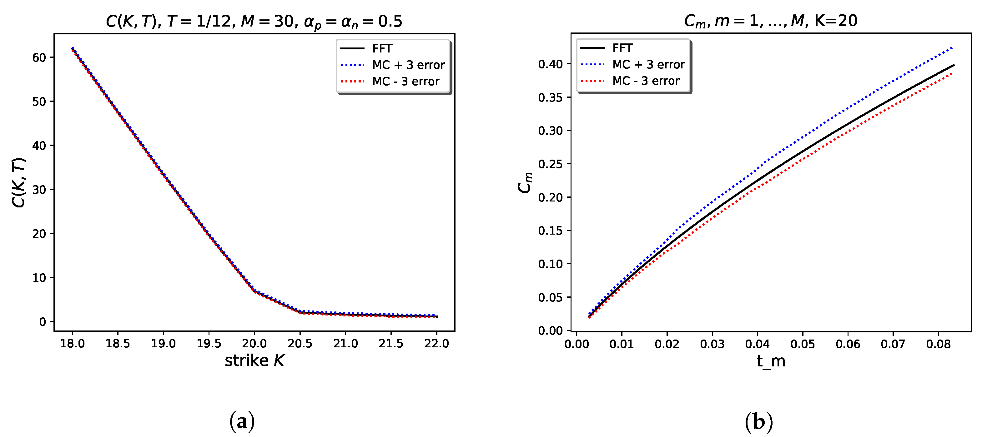
$0.9$		$12.108$	$12.192$	$12.322$	$12.535$	$12.907$

shows the values relative to a strip of $M=30$ daily at-the-money call options with maturity $T=1/12$ with different pairs of ${\alpha }_p,{\alpha }_n$. We observe that fixing one of ${\alpha }_p$ or ${\alpha }_n$, the value of the option is increasing when the other one increases. Moreover, Figure 1a illustrates the variability of the option price with respect to the strike price K, where the dotted lines represent the values obtained with $N={10}^5$ MC simulations plus and minus three times the estimation error (the root-mean squared error divided by $\sqrt{N}$). In addition, Figure 1b compares the price of at-the-money options $C_m=c_m(K,t_m),m=1,\cdots ,M$, $K=20$ obtained with the FFT method with those estimated once again with $N={10}^5$ MC simulations. In these last two examples, we selected ${\alpha }_p={\alpha }_n=0.5$.

As far as the MC method is concerned, the simulation of the skeleton of the process is accomplished running the procedure explained in Sabino and Cufaro Petroni (2022) based on Proposition 4 two times because of the bilateral OU-BCTS; the acceptance rejection step to draw from the law of V in (15) assumes a piecewise approximation of the dominating functions into $L=1000$ terms. The results calculated with the FFT method and with the MC method are totally consistent. On the other hand, it is well-known that the FFT approach is faster. Indeed, they can price vectors of strike prices, thus accelerating the process a lot. Nevertheless, a side product of the MC approach are percentiles or other statistics, which are widely used by practitioners for risk-management purposes.

5.2. Asian Options

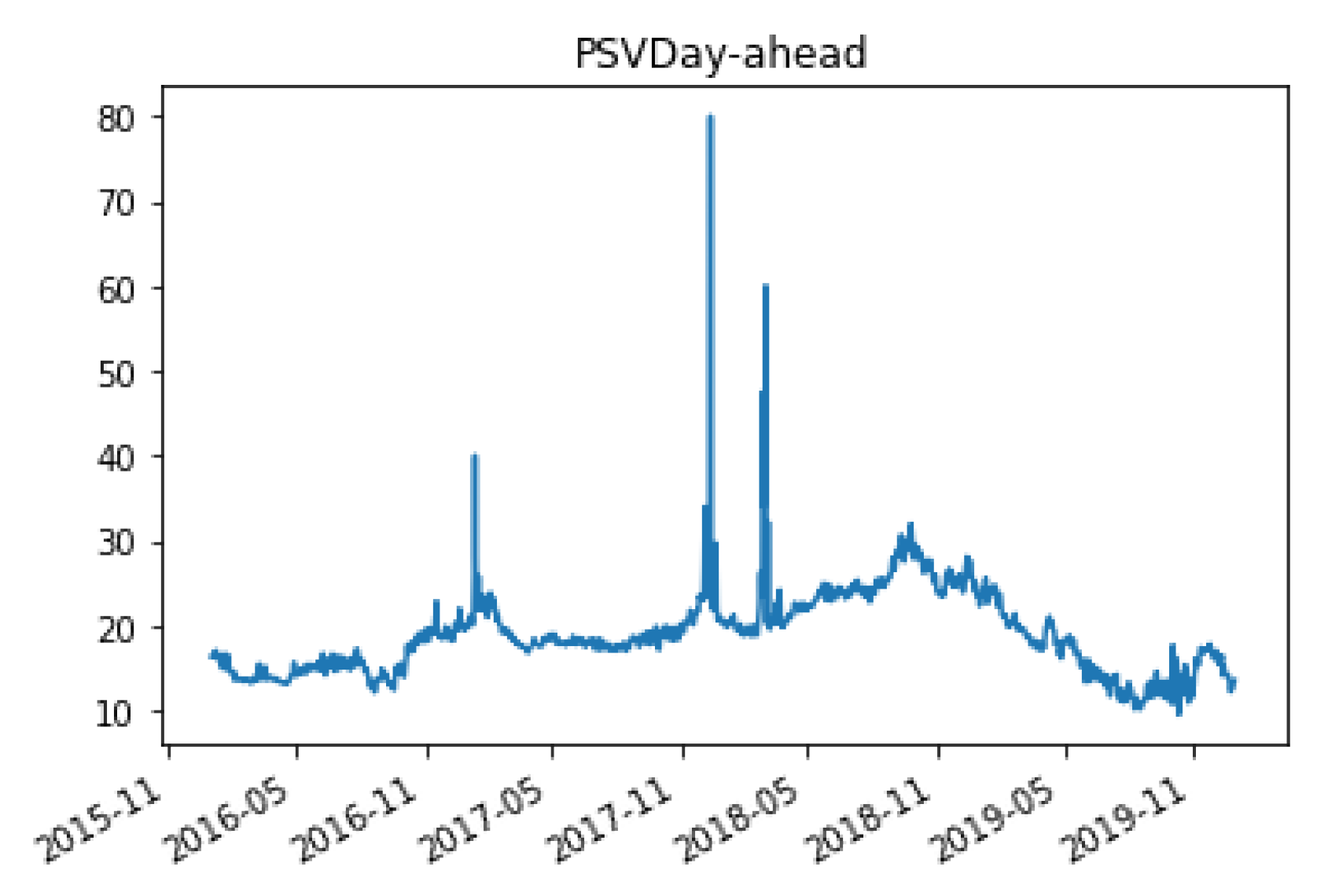
As a second financial application, we consider the pricing of Asian options. In contrast to the previous example, we assume that the market dynamic is driven by an OU-CGMY process with infinite activity and finite variation with $C=c_p=c_n$, $G={\beta }_n$, $M={\beta }_p$ and $Y={\alpha }_p={\alpha }_n$ that we estimate from real data. We consider historical day-ahead prices of the Italian gas market PSV in the four-year time window from 1 January 2016 to 31 December 2019 for a total of 1461 values, see Figure 2.

PSV is the main meeting point between supply and demand of the gas market in Italy. Here, the wholesale gas price is defined, and on the basis of this value, the gas suppliers evaluate the price of the gas raw material to be applied to end customers. There are two main types of contracts between market operators: take or pay and spot, and we focus on the latter type. Spot contracts are signed in the hubs, that is the hubs between the natural gas pipelines, usually located on the border between two states. The gas prices in Europe are strongly interdependent; therefore, the PSV price is affected by the evolution of the main gas prices in Europe, e.g., the Dutch TTF and the German THE and, of course, their values are also influenced by LNG and oil prices as well as from gas imports, e.g., from Algeria and Russia.

As mentioned, in this paper we rely on the reduced-form process approach which consists of specifying a stochastic process for the price evolution from a parameterized family of mean-reverting processes (see Eydeland and Wolyniek 2002). Similar examples including different commodity types can be traced back to Schwartz (1997), who studied oil prices, and after to Benth and Šaltyté Benth (2004), with applications to UK spot gas and Brent crude oil spot prices, or to Geman (2007) for natural gas and oil prices. Alternatively, one could adopt the different point of view of fundamental and hybrid models with a stronger focus on price forecasting rather that on risk-neutral pricing and hedging. To this end, the recent study by Berrisch and Ziel (2002) gives a rigorous data analysis of European gas prices, including the impact of autocorrelation, seasonality, risk premia, temperature, storage levels and the price of European Emission Allowances and the related fuel prices of oil, coal and electricity.

Coming back to the calibration problem, firstly, we check if the time- eries of the logarithm of the day-head prices is nonstationary using the augmented Dickey–Fuller test. On the selected dataset, it turns out that the ADF Statistic is $-1.791886$ with p-value equal to $0.384497$ and with critical values $-3.435$, $-2.864$ and $-2.568$ relative to $1\%, 5\%$ and $10\%$, respectively. Hence, we have to accept the null hypothesis that the time series is nonstationary and does have a time-dependent structure.

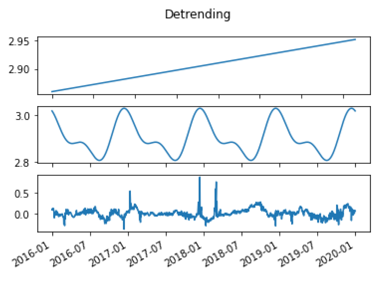
Consequently, we remove the seasonality component from the logarithm of the day-ahead time series using a decomposition with a double cosine plus a linear trend, see Figure 3. Secondly, we assume that the residuals of the deseasonalized time series, denoted $s_k$, $k=1,\cdots ,1461$, follow an autoregressive model AR(1)

$$s_{k+1}=a{s}_k+{ϵ}_{k+1},a=e^{-b\Delta t},$$

(36)

where $\Delta t=1/365$ (one day) and ${ϵ}_k,k=1,\cdots$ is distributed according to the law of $Z(\Delta t)=Z_p(\Delta t)-Z_n(\Delta t)$ in (4) of an OU-CGMY process. The mean reversion rate b can be estimated using the standard least-squares method, however, according to Proposition 1, the pdf of $Z(\Delta t)$ is not known in closed form; therefore, one has to resort to MC-based techniques or to a generalized method of moments. On the other hand, before performing the parameter estimation, we Taylor expand ${\mathrm{\Lambda }}_a$ in Proposition 1

$${\mathrm{\Lambda }}_a=\frac{c\mathrm{\Gamma }(1-\alpha )b{\beta }^{\alpha }}{2}\Delta t^2+o\left(\Delta t^2\right)$$

and observe that for $\Delta t$ small, $X_2$ in Proposition 1 can be neglected (accordingly for the bilateral case), which is reasonable for $\Delta t=1/365$. It turns our that under this approximation, labeled Approximation 1, $Z(\Delta t)\sim \mathcal{BCTS}\left(Y,Y,\frac{M}{a},\frac{G}{a},C\frac{1-a^Y}{Yb},C\frac{1-a^Y}{Yb}\right)$, and we estimate the model parameters adapting the generalized method of moments to match the first four cumulants in (28) and (29), namely, we perform the constrained optimization

$$(\widehat{C},\widehat{G},\widehat{M},\widehat{Y})=\mathrm{arg\; min}\sum _i^4{(c_i(Y,G,M,Y)-\widehat{c_i})}^2,0<Y<1,G>0,M>1,C>0.$$

Table 6. Calibrated parameters.

$\widehat{\mathit{b}}$	$\widehat{\mathit{C}}$	$\widehat{\mathit{G}}$	$\widehat{\mathit{M}}$	$\widehat{\mathit{Y}}$
$75.26$	$4.401$	$3.282$	$3.300$	$0.730$

shows the estimated parameters, whereas

Table 7. Estimated Cumulants times ${10}^3$.

${\widehat{\mathit{c}}}_1$	${\widehat{\mathit{c}}}_2$	${\widehat{\mathit{c}}}_3$	${\widehat{\mathit{c}}}_4$	${\overline{\mathit{c}}}_1$	${\overline{\mathit{c}}}_2$	${\overline{\mathit{c}}}_3$	${\overline{\mathit{c}}}_4$
$0.0409$	$3.985$	$0.0007$	$0.8821$	$-0.0435$	$3.848$	$0.0018$	$0.8374$

reports the sample cumulants $\widehat{c_i},i=1,\cdots ,4$ and the fitted cumulants ${\overline{c}}_i=c_i(\widehat{C},\widehat{G},\widehat{M},\widehat{Y}),i=1,\cdots ,4$. The fit is in agreement with the sample cumulants, taking into account that the first and the fourth ones are very much close to zero.

We now come back to the initial problem of the pricing of Asian options with MC simulation. MC methods are known to be much slower than FFT techniques that can also be tailored to the pricing of Asian options (see Zhang and Oosterlee 2013b). Nevertheless, the former approach provides a view on the distribution of the potential cash flows of derivative contracts, giving precious information to risk managers or to trading units.

We recall that the payoff at maturity T of an Asian option with European style and strike price K is

$$A(K,T)={\left(\frac{{\sum }_{i=1}^{I}S\left(t_i\right)}{I}-K\right)}^{+}.$$

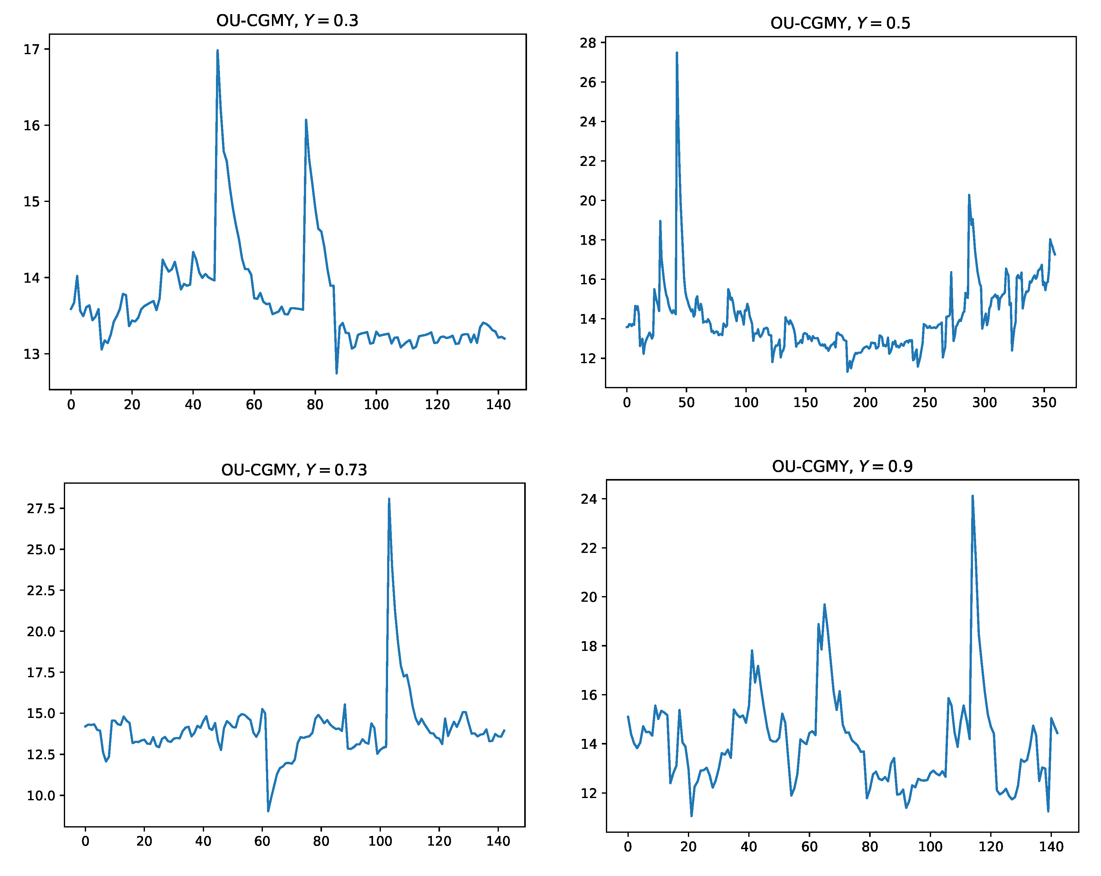
Figure 4 displays a sample of four trajectories with these parameters generated using the procedure of Sabino and Cufaro Petroni (2022), where we also let Y vary.

In addition to this simulation procedure, we consider here two approximations: the first one is Approximation 1 defined in the parameter estimation; the second one—as also assumed in Benth et al. (2018) dealing with the normal inverse Gaussian-driven OU processes—takes advantage of the approximation of the law of $Z(\Delta t)$ with that of $aL(\Delta t)\sim \mathcal{BCTS}\left(Y,Y,\frac{M}{a},\frac{G}{a},C\Delta t,C\Delta t\right)$, $a=e^{-b\Delta t}$ (Approximation 2).

In order to highlight the differences between the estimations returned by the exact method and those with the two alternatives, we consider two Asian options, both of them with $I=90$ daily settlements. The second option, however, is a forward start contract whose first settlement date occurs after 30 days. The MC option values, their relative errors and computational times in seconds are reported in

Table 8. Asian option. $K=13.5$, $T=1/4$.

	Exact		Approx 1		Approx 2		Exact		Approx 1		Approx 2
N	Price (Error)	CPU	Price (Error)	CPU	Price (Error)	CPU	Price (Error)	CPU	Price (Error)	CPU	Price (Error)	CPU
	$Y=0.3$						$Y=0.5$
${10}^3$	0.3293 (0.0091)	0.5	0.3771 (0.0090)	0.3	0.3671 (0.0087)	0.3	0.4439 (0.0107)	0.3	0.4461 (0.0094)	0.2	0.4865 (0.0088)	0.2
${10}^4$	0.3894 (0.0030)	2.7	0.3709 (0.0027)	2.1	0.3655 (0.0028)	2.1	0.4699 (0.0034)	1.5	0.4673 (0.0031)	1.4	0.4499 (0.0029)	1.4
$2\times {10}^4$	0.3692 (0.0022)	5.1	0.3743 (0.0019)	4.0	0.3651 (0.0020)	4.0	0.4571 (0.0024)	2.7	0.4404 (0.0022)	2.8	0.4552 (0.0021)	2.8
$5\times {10}^4$	0.3808 (0.0014)	11.3	0.3814 (0.0012)	9.9	0.3718 (0.0013)	10.0	0.4634 (0.0015)	7.8	0.4594 (0.0014)	6.8	0.4545 (0.0013)	6.8
${10}^5$	0.3792 (0.0010)	22.3	0.3715 (0.0009)	20.0	0.3697 (0.0009)	20.1	0.4627 (0.0011)	15.4	0.4559 (0.0010)	14.0	0.4467 (0.0009)	13.8
	$Y=0.7$						$Y=0.9$
${10}^3$	0.5446 (0.0109)	0.5	0.5317 (0.0104)	0.3	0.5298 (0.0106)	0.3	0.6910 (0.0125)	0.5	0.7031 (0.0108)	0.3	0.7246 (0.0114)	0.3
${10}^4$	0.5902 (0.0035)	2.7	0.5630 (0.0032)	2.1	0.5545 (0.0032)	2.1	0.7102 (0.0038)	2.8	0.7227 (0.0035)	2.4	0.6912 (0.0037)	2.4
$2\times {10}^4$	0.5851 (0.0025)	5.5	0.5631 (0.0023)	4.1	0.5544 (0.0024)	4.3	0.7147 (0.0026)	5.4	0.7066 (0.0025)	4.7	0.6973 (0.0026)	4.7
$5\times {10}^4$	0.5647 (0.0016)	13.1	0.5631 (0.0014)	10.5	0.5413 (0.0015)	10.5	0.7209 (0.0017)	13.7	0.6933 (0.0016)	11.8	0.692 (0.0016)	11.7
${10}^5$	0.5701 (0.0011)	28.0	0.5603 (0.0010)	20.5	0.5491 (0.0010)	21.1	0.7148 (0.0012)	30.3	0.7117 (0.0011)	23.1	0.6897 (0.0012)	24.2

and

Table 9. Forward start Asian option. $K=13.5$, $T=1/3$.

	Exact		Approx 1		Approx 2		Exact		Approx 1		Approx 2
N	Price (Error)	CPU	Price (Error)	CPU	Price (Error)	CPU	Price (Error)	CPU	Price (Error)	CPU	Price (Error)	CPU
	$Y=0.3$						$Y=0.5$
${10}^3$	0.1796 (0.0084)	0.5	0.1452 (0.0075)	0.3	0.1456 (0.0079)	0.3	0.1951 (0.0093)	0.3	0.1698 (0.0084)	0.0	0.1608 (0.0079)	0.2
${10}^4$	0.1740 (0.0027)	2.9	0.1430 (0.0023)	2.1	0.1391 (0.0024)	2.2	0.2020 (0.0030)	1.7	0.1640 (0.0027)	0.1	0.1624 (0.0026)	1.5
$2\times {10}^4$	0.1777 (0.0019)	5.6	0.1394 (0.0017)	4.1	0.1448 (0.0017)	4.1	0.1995 (0.0021)	3.0	0.1629 (0.0018)	0.2	0.1588 (0.0018)	2.9
$5\times {10}^4$	0.1765 (0.0012)	12.6	0.1397 (0.0010)	10.4	0.1445 (0.0011)	10.3	0.2009 (0.0013)	7.7	0.1648 (0.0012)	0.5	0.1578 (0.0011)	7.1
${10}^5$	0.1755 (0.0008)	24.8	0.1415 (0.0007)	20.7	0.1440 (0.0008)	20.7	0.1992 (0.0009)	15.1	0.1633 (0.0008)	1.0	0.1600 (0.0008)	14.3
	$Y=0.7$						$Y=0.9$
${10}^3$	0.2075 (0.0101)	0.5	0.1743 (0.0086)	0.3	0.1970 (0.0094)	0.3	0.2184 (0.0108)	0.5	0.2032 (0.0100)	0.3	0.1788 (0.0101)	0.3
${10}^4$	0.2094 (0.0030)	3.0	0.1754 (0.0027)	2.2	0.1904 (0.0030)	2.2	0.2277 (0.0033)	3.1	0.1863 (0.0030)	2.4	0.1799 (0.0031)	2.5
$2\times {10}^4$	0.2068 (0.0022)	6.1	0.1712 (0.0019)	4.3	0.1778 (0.0020)	4.3	0.2319 (0.0024)	6.0	0.1844 (0.0021)	4.9	0.1849 (0.0022)	4.9
$5\times {10}^4$	0.2102 (0.0014)	14.6	0.1729 (0.0012)	10.8	0.1791 (0.0013)	10.7	0.2252 (0.0015)	15.2	0.1887 (0.0013)	12.0	0.1869 (0.0014)	12.0
${10}^5$	0.2096 (0.0010)	31.1	0.1717 (0.0009)	20.7	0.1797 (0.0009)	21.8	0.2261 (0.0011)	33.7	0.1877 (0.0009)	23.7	0.1840 (0.0010)	24.8

with different Y’s and number of simulations N.

Irrespective to the combination of Y and N, for the option that starts settling after one day, the exact solution and Approximation 1 return very close values, whereas Approximation 2 is slightly biased. In contrast, for the forward start contract, although the time steps for $m>1$ coincide and are very small, for the simple fact that the first time step is relatively high, the estimated prices returned by the two non-xact simulation schemes are quite biased and do not offer an acceptable alternative any longer. More importantly, the bias cannot be controlled by increasing the number of simulations, as shown in Table 9. The cause of this difference it that for forward start options the compound Poisson term cannot be ignored, be it only for one simulation time point, and it is not computationally convenient to simulate 30 extra points with the two approximate methods.

These observations suggest a mixed strategy for parameters estimation and exact simulation of the OU-BCTS processes: Approximation 1 or Approximation 2 for the former task and use the exact and unbiased strategy for the path simulation to avoid being forced to always simulate the process on an unnecessary fine time grid.

5.3. Swing Options

A swing option is a type of contract used by investors in energy markets that lets the option holder buy a predetermined quantity of energy at a predetermined price (strike), while retaining a certain degree of flexibility in both the amount purchased and the price paid.

Let the maturity date T be fixed and the payoff at time $t<T$ be given by ${(S\left(t\right)-K)}^{+}$, where K denotes the strike price. In addition, we assume that only one unit of the underlying can be exercised at any time period. Let $V(n,s,t)$ denote the price of such a swing option at time t given the spot price s which has n out of N exercise rights left. For $m=1,\cdots ,M_S$, the dynamic programming principle allows us to write (see Bertsekas 2005)

$$V(n,s,t_m)=\max \left\{\begin{array}{c}\mathit{E}\left[V(n,S\left(t_{m+1}\right),t_{m+1})|S\left(t_m\right)=s\right],\hfill \\ \\ \mathit{E}\left[V(n-1,S\left(t_{m+1}\right),t_{m+1})|S\left(t_m\right)=s\right]+{(s-K)}^{+}\hfill \end{array}\right\},0<n<N$$

(37)

and $V(n,s,T)={(S\left(T\right)-K)}^{+}$, $0<n\le N$ and $V(0,s,t)=0$. In order to solve the recursion equation, we rely on the modified version of the LSMC, introduced in Longstaff and Schwartz (2001) and detailed in Boogert and de Jong (2008, 2011), where the continuation value is approximated with a linear regression with $m=1,\cdots ,M_S$

$$\mathit{E}\left[V(n,S\left(t_{m+1}\right),t_{m+1})|S\left(t_m\right)=s\right]\simeq a_0+a_{1}S\left(t_m\right)+\cdots ,+a_B{S}^B\left(t_m\right),n<N.$$

In our experiments, we used simple power polynomials with $B=3$, but the regression may be performed on a different set of basis functions as well (see Boogert and de Jong 2011 for a comparison with other basis functions).

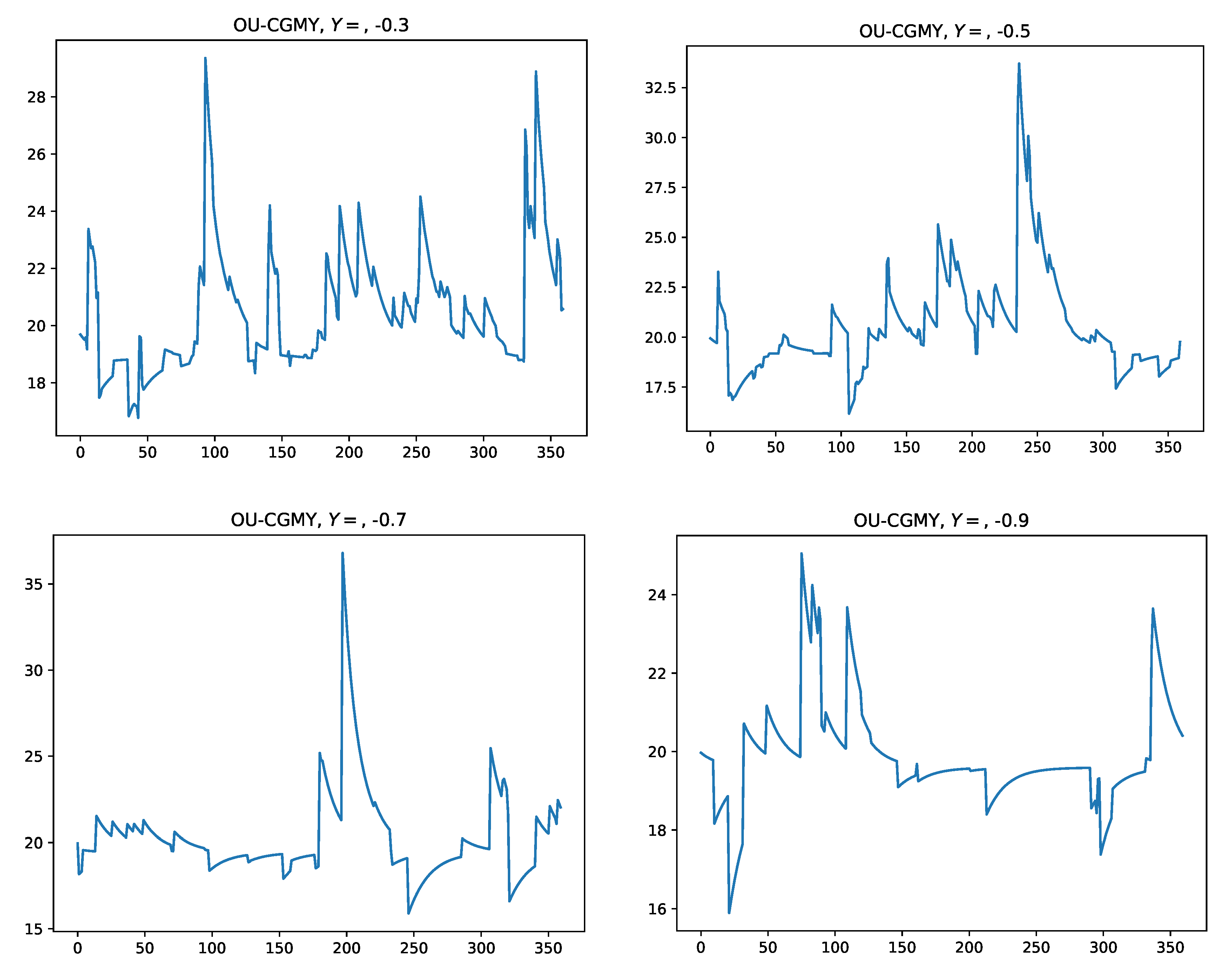
Several other approaches have been proposed: for instance one may solve the recursion by adapting the method of Ben-Ameur et al. (2007) or one might use the quantization technique of Bardou et al. (2009). Alternatively, one can also use the tree method of Jaillet et al. (2004) or the Fourier cosine expansion in Zhang and Oosterlee (2013a) taking advantage of the explicit form of the chf of the OU-BCTS process. On the other hand, a swing contract can be seen as a degenerate case of gas storage, namely with no injection and withdrawal cost equal to the strike (see Boogert and de Jong 2008), and one then could even adopt the recent approach of Boonstra and Oosterlee (2021) based on the COS method. In this last example, we assume an OU-CGMY-driven market model with $Y<0$, namely a combination of mean-reverting compound Poisson processes with positive and negative jumps. We consider a different set of parameters compared with the cases illustrated so far, namely, we take $(b,C,G,M)=(25,80,10.5,15.5)$ and let Y vary. The parameters are very different than the other two examples and are chosen to mimic a realistic price path as shown in Figure 5. We also remark that, due to the fact that energy markets are very seasonal and spikes occur in clusters due to for instance, cold spells, one could assume that the intensity of the compound Poisson processes is a seasonal time-dependent function. The results in Section 3.2 and the simulation algorithms in Section 4 can be easily adapted taking a step-wise approximation of the intensity function.

Table 10. $120-120$ Swing option. $K=20$, $T=1$.

	$\mathit{Y}=0.3$	$\mathit{Y}=0.5$	$\mathit{Y}=0.7$	$\mathit{Y}=0.9$
$\mathit{N}$	Price (Error)	Price (Error)	Price (Error)	Price (Error)
${10}^3$	$101.965$ ($2.873$)	$80.500$ ($2.446$)	$66.634$ ($2.222$)	$51.117$ ($1.983$)
${10}^4$	$99.565$ ($0.902$)	$79.848$ ($0.778$)	$63.451$ ($0.682$)	$49.801$ ($0.599$)
$2\times {10}^4$	$98.328$ ($0.633$)	$79.774$ ($0.550$)	$64.322$ ($0.489$)	$49.958$ ($0.426$)
$5\times {10}^4$	$98.187$ ($0.399$)	$79.585$ ($0.348$)	$63.686$ ($0.307$)	$50.223$ ($0.269$)
${10}^5$	$98.270$ ($0.283$)	$79.284$ ($0.245$)	$63.949$ ($0.217$)	$50.487$ ($0.192$)

shows the values and MC errors relative to the pricing of a $120-120$ swing option with maturity $T=1$ and strike price $K=20$, namely, the holder has $N=120$ rights and can exercise all of them. We also take a flat forward curve $F(0,t)=20,t>0$. The computational time is now dominated by the stochastic optimization, which is independent of the specific price dynamics. On the other hand, the time needed by the path generation is similar to that shown in Table 4. We observe that the LSMC combined with Algorithm 1 produces unbiased results for all selected Y’s, and apparently $2\times {10}^4$ simulations are required to attain an acceptable convergence. In contrast to the Asian option case, it does not make sense to adopt the approximation of the law of $Z\left(t\right)$ in (3) with that of $e^{-kt}L\left(t\right)$ (Approximation 2 in Section 5.2) because this approach returns another compound Poisson process and therefore does not provide a computational advantage.

6. Concluding Remarks

In this study, we investigated the pricing of energy derivatives in markets driven by classical tempered stable and CGMY processes of OU type with finite variation. To this end, we derived the chf of the transition law of such processes in closed form such that we can obtain the nonarbitrage conditions and spot prices that are consistent with the forward curve. In addition, extending the work of Sabino and Cufaro Petroni (2022), we detailed efficient algorithms for the simulation of the skeleton of classical tempered stable and CGMY processes of OU type with particular focus on the case when they coincide with compound Poisson processes. We illustrated the applicability of these results to the pricing of three common derivative contracts in energy markets, namely a strip of daily call options, an Asian option with European style and a swing option. In our numerical experiments, we selected a one-factor model in order to better highlight the features of our finding; nevertheless, the extension to two-factor models in the same vein of Schwartz and Smith (2000) is straightforward. In the first example, we made use of the explicit knowledge of the chf to implement the pricing with the FFT-based technique of Carr and Madan (1999) and compared the outcomes with those obtained via MC simulations. In the second example, we priced Asian options written on the Italian day-ahead gas price PSV with MC simulations, where we also adopted two approximate techniques. These approximations provide reliable values if the time steps of the time grid are relatively small, but if one considers a forward start contract the outcome is really biased. In addition, we showed that the proposed simulation algorithm, combined with the LSMC approach of Boogert and de Jong (2008, 2011), provides an efficient pricing of a one year $120-120$ swing option.

Furthermore, our results are not restricted to OU processes and to the modeling of spot prices. Indeed, in the spirit of Benth et al. (2019), Latini et al. (2019) and Piccirilli et al. (2021), they can be adapted to forward models in order to capture the Samuelson effect and volatility smiles. For instance, Piccirilli et al. (2021) assume that the stochastic evolution of a generic future price at time t, maturity T, $t\le T\le T_1<T_2$ and with delivery period $[T_1,T_2]$ is described by

$$\begin{array}{ccc}\hfill F(t,T_1,T_2)& =& F(0,T_1,T_2)+{\int }_0^t{\mathrm{\Gamma }}_1(u,T_1,T_2)d{L}_1\left(u\right)+{\mathrm{\Gamma }}_2(T_1,T_2)X_2\left(t\right)\hfill \\ & =& F(0,T_1,T_2)+X_1(t,T_1,T_2)+{\mathrm{\Gamma }}_2(T_1,T_2)X_2\left(t\right)\hfill \end{array}$$

where $L_1(·)$ and $X_2(·)$ are two independent Lévy processes. Moreover,

$${\mathrm{\Gamma }}_1(u,T_1,T_2)=\frac{{\gamma }_1}{b(T_2-T_1)}\left(e^{-b(T_1-u)}-e^{-b(T_2-u)}\right),{\mathrm{\Gamma }}_2(T_1,T_2)=\frac{1}{T_2-T_1}{\int }_{T_1}^{T_2}\gamma \left(u\right)du$$

are two deterministic functions that are meant to capture the Samuelson effect in option pricing. Although Piccirilli et al. (2021) illustrate the application of their model under the assumption that $L_1(·)$ and $X_2(·)$ are centered NIG processes, the setting can be modified taking two independent BCTS or CGYM processes. Of course, such models are related to those studied in Section 3, because, after some algebra, it results that

$$X_1(t,T_1,T_2)=\frac{{\gamma }_1}{b(T_2-T_1)}\left(e^{-b(T_1-t)}-e^{-b(T_2-t)}\right){\int }_0^t{e}^{-b(t-u)}d{L}_1\left(u\right)={\mathrm{\Gamma }}_1(t,T_1,T_2)Z\left(t\right).$$

Finally, future studies could cover the extension to a multidimensional framework, for instance adopting the view of Luciano and Semeraro (2010), Ballotta and Bonfiglioli (2013) or the recent approaches of Gardini et al. (2021a, 2021b, 2022) and Lu (2022). A last topic deserving further investigation is the time-reversal simulation of the OU processes generalizing the results of Pellegrino and Sabino (2015) and Sabino (2020b) to the case of classical tempered stable and CGMY processes.

References

1. Ballotta, Laura, and Efrem Bonfiglioli. 2013. Multivariate Asset Models Using Lévy Processes and Applications. The European Journal of Finance 13: 1320–50. [Google Scholar] [CrossRef] [Green Version]
2. Ballotta, Laura, and Ioannis Kyriakou. 2014. Monte Carlo Simulation of the CGMY Process and Option Pricing. Journal of Futures Markets 34: 1095–121. [Google Scholar] [CrossRef] [Green Version]
3. Bardou, Olivier, Sandrine Bouthemy, and Gilles Pagés. 2009. Optimal Quantization for the Pricing of Swing Options. Applied Mathematical Finance 16: 183–217. [Google Scholar] [CrossRef] [Green Version]
4. Barndorff-Nielsen, Ole E. 1998. Processes of Normal Inverse Gaussian Type. Finance and Stochastics 2: 41–68. [Google Scholar] [CrossRef]
5. Barndorff-Nielsen, Ole E., and Neil Shephard. 2001. Non-Gaussian Ornstein-Uhlenbeck-based Models and some of their Uses in Financial Economics. Journal of the Royal Statistical Society: Series B 63: 167–241. [Google Scholar] [CrossRef]
6. Barndorff-Nielsen, Ole E., Jakob L. Jensen, and Michael Sørensen. 1998. Some Stationary Processes in Discrete and Continuous Time. Advances in Applied Probability 30: 989–1007. [Google Scholar] [CrossRef]
7. Ben-Ameur, Hatem, Michéle Breton, Lotfi Karoui, and Pierre L’Ecuyer. 2007. A Dynamic Programming Approach for Pricing Options Embedded in Bonds. Journal of Economic Dynamics and Control 31: 2212–33. [Google Scholar] [CrossRef] [Green Version]
8. Benth, Fred E., and Jüratè Šaltyté Benth. 2004. The Normal Inverse Gaussian Distribution and Spot Price Modelling in Energy Markets. International Journal of Theoretical and Applied Finance 7: 177–92. [Google Scholar] [CrossRef]
9. Benth, Fred E., Jan Kallsen, and Thilo Meyer-Brandis. 2007. A non-Gaussian Ornstein–Uhlenbeck process for electricity spot price modeling and derivatives pricing. Applied Mathematical Finance 14: 153–69. [Google Scholar] [CrossRef]
10. Benth, Fred E., Luca Di Persio, and Silvia Lavagnini. 2018. Stochastic Modeling of Wind Derivatives in Energy Markets. Risks 6: 56. [Google Scholar] [CrossRef] [Green Version]
11. Benth, Fred E., Marco Piccirilli, and Tiziano Vargiolu. 2019. Mean-reverting Additive Energy Forward Curves in a Heath–Jarrow–Morton Framework. Mathematics and Financial Economics 13: 543–77. [Google Scholar] [CrossRef]
12. Berrisch, Jonathan, and Florian Ziel. 2002. Distributional modeling and forecasting of natural gas prices. Journal of Forecasting, 1–22. [Google Scholar] [CrossRef]
13. Bertsekas, Dimitri P. 2005. Dynamic Programming and Optimal Control, Volume I, 3rd ed. Belmont: Athena Scientific. [Google Scholar]
14. Boogert, Alexander, and Cyriel de Jong. 2008. Gas Storage Valuation Using a Monte Carlo Method. Journal of Derivatives 15: 81–91. [Google Scholar] [CrossRef] [Green Version]
15. Boogert, Alexander, and Cyriel de Jong. 2011. Gas Storage Valuation using a Multifactor Price Model. The Journal of Energy Markets 4: 29–52. [Google Scholar] [CrossRef] [Green Version]
16. Boonstra, Boris C., and Cornelis W. Oosterlee. 2021. Valuation of Electricity Storage Contracts Using the COS Method. Applied Mathematics and Computation 410: 126416. [Google Scholar] [CrossRef]
17. Carr, Peter, and Dilip B. Madan. 1999. Option Valuation Using the Fast Fourier Transform. Journal of Computational Finance 2: 61–73. [Google Scholar] [CrossRef] [Green Version]
18. Carr, Peter, and John Crosby. 2010. A Class of Lévy Process Models with almost Exact Calibration to both Barrier and Vanilla FX Options. Quantitative Finance 10: 1115–36. [Google Scholar] [CrossRef]
19. Carr, Peter, Helyette Geman, Dilip B. Madan, and Marc Yor. 2002. The fine structure of asset returns: An empirical investigation. The Journal of Business 75: 305–32. [Google Scholar] [CrossRef] [Green Version]
20. Cartea, Alvaro, and Marcelo G. Figueroa. 2005. Pricing in Electricity Markets: A Mean Reverting Jump Diffusion Model with Seasonality. Applied Mathematical Finance 12: 313–35. [Google Scholar] [CrossRef] [Green Version]
21. Cont, Rama, and Peter Tankov. 2004. Financial Modelling with Jump Processes. London: Chapman and Hall. [Google Scholar]
22. Cufaro Petroni, Nicola. 2008. Self-decomposability and Self-similarity: A Concise Primer. Physica A, Statistical Mechanics and Its Applications 387: 1875–94. [Google Scholar] [CrossRef] [Green Version]
23. Cufaro Petroni, Nicola, and Piergiacomo Sabino. 2020. Pricing exchange options with correlated jump diffusion processes. Quantitative Finance 20: 1811–23. [Google Scholar] [CrossRef]
24. Eydeland, Alexander, and Krzysztof Wolyniek. 2002. Energy and Power Risk Management: New Developments in Modeling, Pricing, and Hedging. Hoboken: Wiley Finance. [Google Scholar]
25. Gardini, Matteo, Piergiacomo Sabino, and Emanuela Sasso. 2021a. A Bivariate Normal Inverse Gaussian Process with Stochastic Delay: Efficient Simulations and Applications to Energy Markets. Applied Mathematical Finance 28: 178–99. [Google Scholar] [CrossRef]
26. Gardini, Matteo, Piergiacomo Sabino, and Emanuela Sasso. 2021b. Correlating Lévy Processes with Self-decomposability: Applications to Energy Markets. Decisions in Economics and Finance 44: 1253–80. [Google Scholar] [CrossRef]
27. Gardini, Matteo, Piergiacomo Sabino, and Emanuela Sasso. 2022. The Variance Gamma++ Process and Applications to Energy Markets. Applied Stochastic Models in Business and Industry 38: 391–418. [Google Scholar] [CrossRef]
28. Geman, Helyette. 2007. Mean Reversion Versus Random Walk in Oil and Natural Gas Prices. Boston: Birkhäuser Boston, pp. 219–28. [Google Scholar] [CrossRef] [Green Version]
29. Grabchak, Michael. 2016. Tempered Stable Distributions. Berlin/Heidelberg: Springer International Publishing. [Google Scholar]
30. Gradshteyn, Iosif S., and Izrail M. Ryzhik. 2007. Table of Integrals, Series, and Products, 7th ed. Amsterdam: Elsevier/Academic Press. [Google Scholar]
31. Hambly, Ben, Samuel Howison, and Tino Kluge. 2009. Modelling Spikes and Pricing Swing Options in Electricity Markets. Quantitative Finance 9: 937–49. [Google Scholar] [CrossRef] [Green Version]
32. Jaillet, Patrick, Ehud I. Ronn, and Stathis Tompaidis. 2004. Valuation of Commodity-Based Swing Options. Management Science 50: 909–21. [Google Scholar] [CrossRef] [Green Version]
33. Jørgensen, Bent. 1997. The Theory of Dispersion Models. London: Chapman & Hall. [Google Scholar]
34. Kallsen, Jan, and Peter Tankov. 2006. Characterization of Dependence of Multidimensional Lévy Processes Using Lévy Copulas. Journal of Multivariate Analysis 97: 1551–72. [Google Scholar] [CrossRef] [Green Version]
35. Koponen, Ismo. 1995. Analytic Approach to the Problem of Convergence of Truncated Lévy Flights Towards the Gaussian Stochastic Process. Phys. Rev. E 52: 1197–99. [Google Scholar] [CrossRef]
36. Küchler, Uwe, and Stefan Tappe. 2013. Tempered Stable Distribution and Processes. Stochastic Processes and Their Applications 123: 4256–93. [Google Scholar] [CrossRef]
37. Latini, Luca, Marco Piccirilli, and Tiziano Vargiolu. 2019. Mean-reverting No-arbitrage Additive Models for Forward Curves in Energy Markets. Energy Economics 79: 157–70. [Google Scholar] [CrossRef]
38. Lawrance, Anthony J. 1980. Some Autoregressive Models for Point Processes. In Point Proceses and Queueing Problems (Colloquia Mathematica Societatis János Bolyai 24). Edited by P. Bartfai and J. Tomko. Amsterdam: North Holland, vol. 24, pp. 257–75. [Google Scholar]
39. Longstaff, Francis A., and Eduardo S. Schwartz. 2001. Valuing American Options by Simulation: A Simple Least-Squares Approach. Review of Financial Studies 14: 113–47. [Google Scholar] [CrossRef] [Green Version]
40. Lord, Roger, F. Fang, Frank Bervoets, and Cornelis W. Oosterlee. 2007. The CONV Method for Pricing Options. PAMM 7: 1024003–4. [Google Scholar] [CrossRef] [Green Version]
41. Lu, Kevin W. 2022. Calibration for Multivariate Lévy-Driven Ornstein-Uhlenbeck Processes with Applications to Weak Subordination. Statistical Inference for Stochastic Processes 25: 365–396. [Google Scholar] [CrossRef]
42. Luciano, Elisa, and Patrizia Semeraro. 2010. Multivariate Time Changes for Lévy Asset Models: Characterization and Calibration. Journal of Computational and Applied Mathematics 233: 1937–53. [Google Scholar] [CrossRef] [Green Version]
43. Madan, Dilip B., and Eugene Seneta. 1990. The Variance Gamma (V.G.) Model for Share Market Returns. The Journal of Business 63: 511–24. [Google Scholar] [CrossRef]
44. Ortiz-Gracia, Luis, and Cornelis W. Oosterlee. 2013. Robust Pricing of European Options with Wavelets and the Characteristic Function. SIAM Journal on Scientific Computing 35: B1055–84. [Google Scholar] [CrossRef] [Green Version]
45. Ortiz-Gracia, Luis, and Cornelis W. Oosterlee. 2016. A Highly Efficient Shannon Wavelet Inverse Fourier Technique for Pricing European Options. SIAM Journal on Scientific Computing 38: B118–43. [Google Scholar] [CrossRef] [Green Version]
46. Pellegrino, Tommaso, and Piergiacomo Sabino. 2015. Enhancing Least Squares Monte Carlo with Diffusion Bridges: An Application to Energy Facilities. Quantitative Finance 15: 761–72. [Google Scholar] [CrossRef]
47. Piccirilli, Marco, Maren D. Schmeck, and Tiziano Vargiolu. 2021. Capturing the Power Options Smile by an Additive Two-factor Model for Overlapping Futures Prices. Energy Economics 95: 105006. [Google Scholar] [CrossRef]
48. Poirot, Jérémy, and Peter Tankov. 2006. Monte Carlo Option Pricing for Tempered Stable (CGMY) Processes. Asia-Pacific Financial Markets 13: 327–44. [Google Scholar] [CrossRef]
49. Qu, Yan, Angelos Dassios, and Hongbiao Zhao. 2021. Exact Simulation of Ornstein–Uhlenbeck Tempered Stable Processes. Journal of Applied Probability 58: 347–71. [Google Scholar] [CrossRef]
50. Rosinski, Jan. 2007. Tempering Stable Proceses. Stochastic Processes and Their Applications 117: 677–707. [Google Scholar] [CrossRef] [Green Version]
51. Sabino, Piergiacomo. 2020a. Exact Simulation of Variance Gamma Related OU Proceses: Application to the Pricing of Energy Derivatives. Applied Mathematical Finance 27: 207–27. [Google Scholar] [CrossRef]
52. Sabino, Piergiacomo. 2020b. Forward or Backward Simulations? A Comparative Study. Quantitative Finance 20: 1213–26. [Google Scholar] [CrossRef]
53. Sabino, Piergiacomo, and Nicola Cufaro Petroni. 2021a. Fast Pricing of Energy Derivatives with Mean-Reverting Jump-diffusion Processes. Applied Mathematical Finance 28: 1–22. [Google Scholar] [CrossRef]
54. Sabino, Piergiacomo, and Nicola Cufaro Petroni. 2021b. Gamma-related Ornstein–Uhlenbeck Processes and their Simulation. Journal of Statistical Computation and Simulation 91: 1108–33. [Google Scholar] [CrossRef]
55. Sabino, Piergiacomo, and Nicola Cufaro Petroni. 2022. Fast Simulation of Tempered Stable Ornstein–Uhlenbeck Processes. Computational Statistics, 1–35. [Google Scholar] [CrossRef]
56. Sato, Ken-iti. 1999. Lévy Processes and Infinitely Divisible Distributions. Cambridge: Cambridge U.P. [Google Scholar]
57. Schwartz, Eduardo S. 1997. The Stochastic Behaviour of Commodity Prices. The Journal of Finance 52: 923–73. [Google Scholar] [CrossRef]
58. Schwartz, Eduardo S., and James E. Smith. 2000. Short-term Variations and Long-term Dynamics in Commodity Prices. Management Science 46: 893–911. [Google Scholar] [CrossRef] [Green Version]
59. Zhang, Bowen, and Cornelis W. Oosterlee. 2013a. An Efficient Pricing Algorithm for Swing Options based on Fourier Cosine Expansions. Journal of Computational Finance 16: 1–32. [Google Scholar] [CrossRef] [Green Version]
60. Zhang, Bowen, and Cornelis W. Oosterlee. 2013b. Efficient Pricing of European-style Asian Options under Exponential Lévy Processes based on Fourier Cosine Expansions. SIAM J. Financial Math. 4: 399–426. [Google Scholar] [CrossRef]
Figure 1. Call option values calculated with FFT and MC with N = 10 5 , ( b , β p , β n , c p , c n ) = ( 0.1 , 2.5 , 3.5 , 0.5 , 1 ) , α p = α n = 0.5 , K = 20 . (a) Effect on the strike; (b) c m ( K , t m ) , m = 1 , , 30 .
Risks 10 00148 g001
Figure 2. Day-ahead PSV prices.
Risks 10 00148 g002
Figure 3. Detrending.
Risks 10 00148 g003
Figure 4. Sample trajectories of OU-CGMY processes with b , C , G , M = 75.26 , 4.401 , 3.382 , 3.300 and Y { 0.3 , 0.5 , 0.73 , 0.9 } .
Risks 10 00148 g004
Figure 5. Sample trajectories of OU-CGMY processes with b , C , G , M = 10 , 10 , 1.75 , 1.25 and Y { 0.3 , 0.5 , 0.7 , 0.9 } .
Risks 10 00148 g005